Empirical Bolometric Correction Coefficients for Nearby Main-Sequence Stars in Gaia Era

Abstract

Nearby detached double-lined eclipsing binaries with most accurate data were studied and 290 systems were found with at least one main-sequence component having a metallicity $0.008\leq Z\leq 0.040$. Stellar parameters, light ratios, Gaia DR2 trigonometric parallaxes, extinctions and/or reddening were investigated and only 206 systems were selected eligible to calculate empirical bolometric corrections. NASA-IPAC Galactic dust maps were main source of extinctions. Unreliable extinctions at low Galactic latitudes $|b|\leq 5^{o}$ were replaced with individual determinations, if they exist in the literature, else associated systems are discarded. Main-sequence stars of remaining systems were used to calculate bolometric corrections ($BC$) and to calibrate $BC-T_{eff}$ relation, which is valid in the range 3100-36000 K. De-reddened $(B-V)_{0}$ colours, on the other hand, allowed us to calibrate two intrinsic colour effective temperature relations, where the linear one is valid for $T_{eff}>10000$ K, while the quadratic relation is valid for $T_{eff}<10000$ K, that is, both are valid in the same temperature range $BC-T_{eff}$ relation is valid. New $BC$ computed from $T_{eff}$ and other astrophysical parameters are tabulated, as well.

1 Introduction

Outstanding improvements in stellar astrophysics have been recorded in recent years. High sensitivity images taken with satellite telescopes, data obtained with advanced new technology telescopes and high-resolution spectrographs have an important share in this. While advanced analysis techniques were added to these advances, the basic astrophysical parameters began to be obtained very precisely (especially close to 1% precision in the mass and radius of double-lined detached binaries). On the other hand, it is important for many purposes to obtain the total luminosity or bolometric brightness of stars. Bolometric corrections ($BC$) are necessary to derive the total luminosity. Luminosity, however, is typically measured in a given bandpass (or a few bandpasses). To pass from luminosity in a given band to total luminosity, $BC$s are needed.

Historically, a $BC$ for a star is defined as the difference between its bolometric and visual magnitudes as,

$$BC=M_{Bol}-M_{V}=m_{Bol}-m_{V},$$ (1)

where subscripts “Bol” and “V” imply bolometric and visual bandwidths if $M$ is the absolute and $m$ is the apparent magnitudes. Here, the preference of the visual band is the convention because throughout the history visual magnitudes are mostly used and mostly available.

Since there is no telescope or a detector to observe a star at all wavelengths and because the bolometric magnitude of the star is related to its luminosity by the relation,

$$M_{Bol}=M_{Bol,\odot}-2.5\log L/L_{\odot},$$ (2)

where $M_{Bol,\odot}$ and $L_{\odot}$ are the reference quantities representing the bolometric magnitude and the luminosity of the Sun, then $BC$ is a correction for the missing luminosity. Similarly, apparent magnitude of the star is related to its flux ($f$) just above the atmosphere by the relation

$$m_{V}=-2.5\log f_{V}+C_{V},$$ (3)

where $C_{V}$ and $f_{V}$ are the zero point constant and the flux received from this star, thus $BC$ may also be understood as the missing flux which cannot be observed due to limited observable bandwidth.

There is a large body of works on this topic. Notable early ones are summarized by Kuiper (1938) and Popper (1959). Most works used Spectral Energy Distribution (SED) in different bands, typically given in tabular forms (McDonald & Underhill, 1952; Heintze, 1973; Code et al., 1976; Malagnini et al., 1985; Cayrel et al., 1997; Bessell, Castelli & Plez, 1998; Girardi et al., 2008), and some used radiometric measurements (Pettit & Nicholson, 1928; Wildey, 1963), while some preferred classical photometric methods to derive $BC$s together with intrinsic colours (Johnson, 1964, 1966; Flower, 1977, 1996; Sung et al., 2013). Recently, synthetic stellar photometry and theoretical spectral libraries has been also preferred to drive various kinds of $BC$s (Casagrande & VandenBerg, 2018; Chen et al., 2019).

In recent years, one of the most used paper is that of Flower (1996), who gives three empirical $BC-T_{eff}$ relations each valid at three different temperature ranges, but usable for all luminosity classes (see also, Torres, 2010). Here we want to improve upon the work of Flower (1996) including recently compiled more reliable data in order to test the claim of if a single empirical $BC-T_{eff}$ relation would be valid or not for all stellar temperatures and for all spectral classes. We take the advantage of Gaia, which provides the most precise and accurate stellar parallaxes ever measured, and the numerous more accurate data which was gathered since then. For this study, we start with obtaining empirical $BC$ coefficients of nearby main-sequence stars.

Using the most reliable stellar basic parameters ($M$, $R$, $T_{eff}$), and Gaia DR2 trigonometric parallaxes of the detached double-lined eclipsing binaries (Gaia Collaboration et al., 2016, 2018) and interstellar extinction ($A_{V}$) partly from the NASA/IPAC Galactic dust maps (Schlafly & Finkbeiner, 2011) partly from private determinations, $BC$ coefficients for Solar neighborhood main-sequence stars are determined and a new $BC-T_{eff}$ relation is calibrated in this study. This new relation is more practical (with less number of digits) compared to the coefficients of the rectified relations by Torres (2010) and it is a single fourth degree polynomial valid for the temperature range 3100-36000 K.

2 Data

An absolute bolometric magnitude of a star could be computed by Eq. (2) using the reference quantities $M_{Bol}=4.74$ mag and $L_{\odot}=3.828\times 10^{26}$ W according to IAU 2015 General Assembly resolution B2. However, a luminosity of a star is not one of its directly observable parameters, but it is an empirical parameter which has to be computed from observable parameters: the radius ($R$) and the effective temperature ($T_{eff}$) using the following relation

$${\frac{L}{L_{\odot}}}=\left({\frac{R}{R_{\odot}}}\right)^{2}\left({\frac{T_{eff}}{T_{eff,\odot}}}\right)^{4},$$ (4)

in accord with the Stefan-Boltzmann law. Since stellar temperatures are in Kelvin and stellar radii are in Solar units, $T_{eff,\odot}=5772$ K is also needed according to IAU 2015 General Assembly resolution B3.

It is clear that when computing an empirical $BC$ of a star, a reliable observational $R$ and a trustable $T_{eff}$ are needed in the first step to obtain its $M_{Bol}$. Next a reliable apparent visual magnitude ($m_{V}$), a distance ($d$) and an extinction ($A_{V}$) in the visual band are necessary for the second step according to

$$m_{V}-M_{V}=5\log d-5+A_{V},$$ (5)

from where visual absolute magnitude ($M_{V}$) of the star could be extracted. Finally $M_{Bol}$ and $M_{V}$ would be ready to apply Eq. (1).

2.1 Selecting stars for the first step

Since most accurate stellar parameters ($M$, $R$, $T_{eff}$) come from simultaneous solutions of observed light and radial velocity curves of detached double-lined eclipsing binaries, main source of data for this study is “The Catalogue of Stellar Parameters from the Detached Double-lined Eclipsing Binaries in the Milky Way” which was originally compiled by Eker et al. (2014). Although the steps described are applicable to all stars, only main-sequence stars were chosen for this study because the number of stars out of the main-sequence in the catalogue are insufficient to explore their $BC-T_{eff}$ relations.

The original catalogue of Eker et al. (2014) is updated and the number of systems is increased to 319 (318 SB2 and one SB3) by Eker et al. (2018), who selected 509 stars with $M$ and $R$ both accurate up to 15% and metallicities ($0.008\leq Z\leq 0.040$) in order to calibrate interrelated main-sequence mass-luminosity (MLR), mass-radius (MRR) and mass-effective temperature (MTR) relations for the Galactic nearby stars. Therefore, the list already prepared by Eker et al. (2018) is considered to be the initial list for the present study.

Unfortunately, not all stars with $M$ and $R$ accuracies within 15% and metallicities within $0.008\leq Z\leq 0.040$ in the catalogue have published $T_{eff}$. This is because some authors, such Young et al. (2006), Shkolnik et al. (2008), Hełminiak et al. (2009) and Sandquist et al. (2013), prefer to give temperature ratios rather than individual temperatures of the components in their publication. 53 stars (25 SB2 and 1 SB3) without published $T_{eff}$ were eliminated right at the beginning; that is, not included in the calibrations of interrelated MLR, MRR and MTR. For this study, we have re-explored those 53 stars and found 34 of them fulfilling the both conditions that $M$ and $R$ are both accurate up to 15% and metallicities $0.008\leq Z\leq 0.040$ on the main-sequence region of the $\log M-\log R$ diagram defined by zero age main-sequence (ZAMS) and terminal age main-sequence (TAMS) lines according to PARSEC stellar evolution models (Bressan et al., 2012). Now, these stars too are included in the list of stars collected for the first step. This is because; it is now possible to assign them a reliable $T_{eff}$ according to the basic relations MLR, MRR and MTR.

Recently, Graczyk et al. (2019) studied the global zero-point shift between the photometric parallaxes of 81 detached eclipsing binaries and Gaia Data Release 2 (DR2) trigonometric parallaxes (Gaia Collaboration et al., 2018). 72 of those binaries are already in our catalog. The paper of Graczyk et al. (2019) contained more, that is, additional seven systems (AL Ari, AL Dor, V530 Ori, KX Cnc, V923 Sco, TYC 7091-888-1, EPIC 211409263) with accurately determined $R$ and $T_{eff}$ from light and radial velocity curves using Wilson-Devinney code version 2007 (van Hamme & Wilson, 2007). We decided also to include those seven systems into the list of stars for the first step. Finally, the number of stars is maximized to 550 stars, which their absolute bolometric magnitude could be computed from their $R$ and $T_{eff}$ according to (2) and (4) for the first step of computing $BC$.

2.2 Selecting systems for the second step

The number of stars is maximized in the first step above because this number would be decreased greatly in the second step. The loss is inevitable because it is not possible to calculate absolute visual magnitude $M_{V}$ of a star if any of the observational parameters $m_{V}$, $d$ or $A_{V}$ is absent. Moreover, rather than counting individual stars, counting binary systems is more meaningful in the second step. This is because if an extinction ($A_{V}$) or a distance ($d$) is missing, it is missing for the system, not only for one star. Furthermore, apparent visual magnitude of a component ($m_{V}$) is available only if a reliable light ratio ($L_{2}/L_{1}$) of the components in the visual band is available. Thus, systems without ($L_{2}/L_{1}$) in the $V$ band are also lost. Therefore, chosen stars organized as systems. Consequently, we have counted 290 systems, which have at least one component on the main-sequence.

We went through each system and have been able to select 206 systems with complete data to calculate both $M_{Bol}$ and $M_{V}$, that is, $BC$ is computable. The basic observational parameters of 206 systems are given in Table 1. The columns are self-explanatory and organized as: ID number, name of the system, equatorial coordinates ($\alpha$, $\delta$; International Celestial Reference System in J2000.0), Galactic coordinates ($l$, $b$), spectral types, orbital periods ($P$), references, $B$ magnitudes and errors, $V$ magnitudes and errors, references, interstellar extinction in $V$ band ($A_{V}$) and its error, references, trigonometric parallaxes and errors, references.

NASA/IPAC Galactic Dust Reddening and Extinction maps are our main source for $A_{V}$ data listed in Table 1. This web site provides an extinction map, the corresponding 100 micron intensity, and dust temperature, along with statistics for each if Galactic coordinates of an object is provided. A $E(B-V)$ colour-excess and associated error towards the direction of a star, from the Sun up to the Galactic border, due to the dust in the Milky Way disk are taken from Schlafly & Finkbeiner (2011), who assume a single standard extinction law $A_{V}=3.1E(B-V)$. Consequently, corresponding total extinction (from Sun up to Galactic border) and associated error for the $V$ band are known. The total extinction ($A_{\infty}(b)$) is then reduced for the distance of the star by using the relation of Bahcall & Soneira (1980),

$$A_{d}(b)=A_{\infty}(b)\Biggl{[}1-\exp\Biggl{(}\frac{-\mid d~{}\sin(b)\mid}{H}\Biggr{)}\Biggr{]},$$ (6)

where $b$ is the Galactic latitude, $d$ is the distance of the system from the Sun. $H$ is the Galactic dust scaleheight ($H$=125 pc; Marshall et al., 2006), Only, the two systems, $\beta$ Aur and V2083 Cyg, do not have Gaia trigonometric parallax measurements because they are too bright for Gaia detectors. We did not want to discard them, instead use them with their Hipparcos trigonometric parallaxes (van Leeuwen, 2007). There are 12 more systems which we also preferred to use their Hipparcos trigonometric parallaxes. Those are the systems which are brighter than $V=8$ mag and having hot components (spectral types A or earlier).

It is clear by Eq. (6) that, extinctions of the systems with low-Galactic latitudes ($|b|<5^{o}$) are unreliable, especially if $d$ is large ($d>100$ pc). Such systems are more likely to be embedded in the dust concentrated in the Galactic plane. Therefore, for the systems with relatively low-Galactic latitudes and for the systems with large reddening, we have searched in the literature if their $E(B-V)$ colour excess is measured by other authors. If there is an observationally determined value of $A_{V}$ or $E(B-V)$, we have preferred them rather than our estimates according to NASA/IPAC Galactic Dust Reddening and Extinction maps. Some systems with hotter components, spectral types A or earlier, we could not find any privately determined $A_{V}$ or $E(B-V)$, but we were able to use $Q$ method (Johnson & Morgan, 1953) to estimate their $E(B-V)$ and $A_{V}$. If $Q$ method is not applicable (systems of late spectral types) and if there is no published $A_{V}$ or $E(B-V)$ for a system, then it is discarded because of unreliable $A_{V}$. Among the 206 system listed in Table 1, there are 131 systems with $A_{V}$, which is estimated from the Galactic dust maps, and rest (75 systems) are from the $E(B-V)$ colour-excess measurements by the authors referenced in the table. Extinctions relying on $Q$ method are referenced to “this study”.

Table 2 gives the rest of the other parameters which are needed in computing $BC$ values. The columns of Table 2 are organized as: ID number, name of the system, primary mass and its error, secondary mass and its error, primary radius and its error, secondary radius and its error, references, primary effective temperature and its error, secondary effective temperature and its error, references, light ratio ($L_{2}/L_{1}$) in $B$ band, $B$ contribution of the third body if exists, light ratio ($L_{2}/L_{1}$) in $V$ band, $V$ contribution of the third body if exists, references.

Table 1: Basic observational parameters of the detached double-lined eclipsing systems selected.

ID	Name	$\alpha$	$\delta$	$l$	$b$	Spt Type	$P$	Reference	$B$	$V$	Reference	$A_{V}$	Reference	$\varpi$	Reference
		(hh:mm:ss)	(dd:mm:ss)	(o)	(o)		(day)		(mag)	(mag)		(mag)		(mas)
1	V421 Peg	00:07:02.00	+22:50:40.03	109.75	-38.89	F1V + F2V	3.087566	2007A&A…474..653V	—	8.280$\pm$0.010	2016NewA…46…47O	0.158$\pm$0.005	2011ApJ…737..103S	6.3806$\pm$0.0543	2018A&A…616A…1G
2	DV Psc	00:13:09.20	+05:35:43.06	105.72	-55.99	K4V + M1V	0.30853609	2007MNRAS.382.1133Z	11.604$\pm$0.010	10.621$\pm$0.010	2000A&A…355L..27H	0.012$\pm$0.001	2011ApJ…737..103S	0.0120$\pm$0.0787	2018A&A…616A…1G
3	MU Cas	00:15:51.56	+60:25:53.64	118.55	-2.14	B5V + B5V	9.652929	2004AJ….128.1840L	11.112$\pm$0.009	10.808$\pm$0.007	2019ApJ…872…85G	1.249$\pm$0.027	2011ApJ…737..103S	1.2490$\pm$0.0397	2018A&A…616A…1G
4	GSC 4019-3345	00:22:45.37	+62:20:05.50	119.61	-0.35	A4 V + A4 V	4.077304	2013PASA…30…26B	12.550$\pm$0.009	12.150$\pm$0.008	2013PASA…30…26B	0.880$\pm$0.100	This study	0.9513$\pm$0.0316	2018A&A…616A…1G
5	YZ Cas	00:45:39.08	+74:59:17.06	122.55	12.12	A2m + F2V	4.4672235	2014MNRAS.438..590P	5.715$\pm$0.026	5.660$\pm$0.015	2019ApJ…872…85G	0.195$\pm$0.008	2011ApJ…737..103S	0.1950$\pm$0.0939	2018A&A…616A…1G
…	…	…	…	…	…	…	…	…	…	…	…	…	…	…	…
…	…	…	…	…	…	…	…	…	…	…	…	…	…	…	…
…	…	…	…	…	…	…	…	…	…	…	…	…	…	…	…
200	AR Cas	23:30:01.94	+58:32:56.11	112.47	-2.66	B4V + A6V	6.066317	1999A&A…345..855H	4.777$\pm$0.004	4.893$\pm$0.004	2003ARep…47..551K	0.350$\pm$0.030	2003ARep…47..551K	0.3500$\pm$0.2047	2018A&A…616A…1G
201	V731 Cep	23:37:43.55	+64:18:11.20	115.05	2.57	B8.5V + A1.5V	6.068456	2008MNRAS.390..399B	10.630$\pm$0.008	10.540$\pm$0.008	2008MNRAS.390..399B	0.403$\pm$0.093	This study	0.4030$\pm$0.0305	2018A&A…616A…1G
202	IT Cas	23:42:01.40	+51:44:36.80	112.13	-9.67	F6V + F6V	3.8966721	1997AJ….114.1206L	11.640$\pm$0.019	11.150$\pm$0.039	1997AJ….114.1206L	0.180$\pm$0.030	2016AJ….152..180S	2.0149$\pm$0.0358	2018A&A…616A…1G
203	BK Peg	23:47:08.46	+26:33:59.92	105.53	-34.12	F8	5.48991046	1983AJ…..88.1242P	10.540$\pm$0.041	9.982$\pm$0.010	2019ApJ…872…85G	0.152$\pm$0.004	2011ApJ…737..103S	0.1520$\pm$0.0526	2018A&A…616A…1G
204	AP And	23:49:30.71	+45:47:21.25	111.78	-15.74	F6 + F8	1.587291156	1984ApJS…54..421G	11.606$\pm$0.057	11.074$\pm$0.085	2015AAS…22533616H	0.270$\pm$0.020	2016AJ….152..180S	0.2700$\pm$0.0415	2018A&A…616A…1G
205	AL Scl	23:55:16.58	-31:55:17.28	8.14	-76.89	B6V + B9V	2.445083	1987A&A…179..141H	5.985$\pm$0.014	6.070$\pm$0.009	2000A&A…355L..27H	0.100$\pm$0.010	This study	4.2680$\pm$0.1273	2018A&A…616A…1G
206	V821 Cas	23:58:49.17	+53:40:19.82	115.10	-8.4	A1.5V + A4V	1.7697999	2009MNRAS.395.1649C	8.402$\pm$0.029	8.286$\pm$0.017	2019ApJ…872…85G	0.217$\pm$0.009	2011ApJ…737..103S	0.2170$\pm$0.0376	2018A&A…616A…1G

Table 2: Physical parameters of selected systems which are necessary in computing their $BC$.

										$B$ Band		$V$ Band
ID	Name	$M_{1}$	$M_{2}$	$R_{1}$	$R_{2}$	Reference	$T_{1}$	$T_{2}$	Reference	$L_{2}/L_{1}$	$L_{3}$	$L_{2}/L_{1}$	$L_{3}$	Reference
		($M_{\odot}$)	($M_{\odot}$)	($R_{\odot}$)	($R_{\odot}$)		(K)	(K)
1	V421 Peg	1.594$\pm$0.029	1.356$\pm$0.029	1.584$\pm$0.028	1.328$\pm$0.029	2016NewA…46…47O	7250$\pm$80	6980$\pm$120	2016NewA…46…47O	—	—	0.6023	—	2016NewA…46…47O
2	DV Psc	0.677$\pm$0.019	0.475$\pm$0.010	0.685$\pm$0.030	0.514$\pm$0.020	2014PASA…31…24E	4450$\pm$8	3614$\pm$8	2007MNRAS.382.1133Z	0.0893	—	0.1254	—	2014AJ….147…50P
3	MU Cas	4.657$\pm$0.100	4.575$\pm$0.090	4.192$\pm$0.050	3.671$\pm$0.040	2014PASA…31…24E	14750$\pm$500	15100$\pm$500	2004AJ….128.1840L	0.7982	—	0.7957	—	2019ApJ…872…85G
4	GSC 4019-3345	1.920$\pm$0.010	1.920$\pm$0.010	1.760$\pm$0.050	1.760$\pm$0.050	2013PASA…30…26B	8600$\pm$310	8600$\pm$570	2013PASA…30…26B	1.0121	—	1.0161	—	2013PASA…30…26B
5	YZ Cas	2.263$\pm$0.012	1.325$\pm$0.007	2.525$\pm$0.011	1.331$\pm$0.006	2014MNRAS.438..590P	9520$\pm$120	6880$\pm$240	2014MNRAS.438..590P	0.0610	—	0.0880	—	2019ApJ…872…85G
…	…	…	…	…	…	…	…	…	…	…	…	…	…	…
…	…	…	…	…	…	…	…	…	…	…	…	…	…	…
…	…	…	…	…	…	…	…	…	…	…	…	…	…	…
200	AR Cas	5.900$\pm$0.200	1.860$\pm$0.060	4.860$\pm$0.100	1.590$\pm$0.030	2014PASA…31…24E	16800$\pm$200	8250$\pm$100	2003ARep…47..551K	0.0205	1.14	0.0304	1.71	2003ARep…47..551K
201	V731 Cep	2.577$\pm$0.098	2.017$\pm$0.084	1.823$\pm$0.030	1.717$\pm$0.025	2014PASA…31…24E	10700$\pm$200	9265$\pm$220	2008MNRAS.390..399B	0.5649	—	0.6129	—	2008MNRAS.390..399B
202	IT Cas	1.330$\pm$0.009	1.328$\pm$0.008	1.603$\pm$0.015	1.569$\pm$0.040	2014PASA…31…24E	6470$\pm$110	6470$\pm$110	1997AJ….114.1206L	0.9685	—	0.9646	—	1997AJ….114.1206L
203	BK Peg	1.414$\pm$0.007	1.257$\pm$0.005	1.985$\pm$0.008	1.472$\pm$0.017	2014PASA…31…24E	6265$\pm$85	6320$\pm$30	2010A&A…516A..42C	0.5780	—	0.5721	—	2019ApJ…872…85G
204	AP And	1.277$\pm$0.004	1.251$\pm$0.004	1.234$\pm$0.006	1.195$\pm$0.005	2014AJ….147..148L	6565$\pm$150	6495$\pm$150	2014AJ….147..148L	0.8857	—	0.8904	—	2014MNRAS.437.3718Z
205	AL Scl	3.617$\pm$0.110	1.703$\pm$0.040	3.241$\pm$0.050	1.401$\pm$0.020	2014PASA…31…24E	13550$\pm$350	10300$\pm$360	1987A&A…179..141H	0.0417	—	0.0526	—	1981Ap&SS..74…83G
206	V821 Cas	2.025$\pm$0.066	1.620$\pm$0.058	2.308$\pm$0.028	1.390$\pm$0.022	2014PASA…31…24E	9400$\pm$400	8600$\pm$400	2009MNRAS.395.1649C	0.2550	—	0.2830	—	2019ApJ…872…85G

Mass and radius collected from older references are homogenized and re-evaluated using recently updated and more accurate constants $GM_{\odot}=1.3271244\times 10^{20}$ m³s^-2 (Standish, 1995) and $R_{\odot}=6.9566\times 10^{8}$m (Haberreiter et al., 2008) by Eker et al. (2014). Therefore, absolute parameters $M$, $R$ coming from the older references are given a single reference. Interested readers may follow the references given in Eker et al. (2014) for the original published values. The $GM_{\odot}$ value adopted by Eker et al. (2014, 2015) is the same as the $GM_{\odot}$ value adopted by IAU 2015 General Assembly resolution B3. However, the Solar radius ($R_{\odot}$) is 0.057% smaller than $R_{\odot}=6.957\times 10^{8}$ m which is adopted by IAU 2015. Such a small difference is definitely negligible besides the uncertainties of the observed stellar radii.

The basic astrophysical parameters ($M$, $R$ and $T_{eff}$) of the secondary components of TZ for, Z Her, HD147827, BD-20 5728, EPIC 211409263, NSVS 11868841, NSVS 06502726, NSVS 02502726 and primary components of TYC 7091-888-1, TYC 176-2950-1, V432 Aur and V380 Cyg are not listed in Table 2 because they are not main-sequence stars, thus, they are discarded from this study.

The most critical requirement for a system to be included in this study is to have light ratio ($L_{2}/L_{1}$) in the $V$ band. Without it, apparent brightness’ of the components in the $V$ band cannot be computed, so their $BC$ coefficients. Therefore, all 206 systems have a light ratio ($L_{2}/L_{1}$) for the $V$ band. Originally, we were also interested in $L_{2}/L_{1}$ for the $B$ band in order to estimate un-reddened $B-V$ colours of the components. However, $L_{2}/L_{1}$ for the $B$ band cannot be found for 60 systems. Therefore, only the values of existing $L_{2}/L_{1}$ for the $B$ band are listed in Table 2. Correspondingly, the systemic brightness’ for $B$ band for these systems are also left empty for the same reason in Table 1, not because we could not found $B$ magnitudes for these systems in the literature.

2.3 Main-sequence confirmation of the sample

The positions of 400 stars (194 binaries, 8 primaries, and 4 secondaries) are shown on a $\log M-\log R$ diagram in Fig. 1a, where the ZAMS and TAMS lines of PARSEC stellar evolution models (Bressan et al., 2012) marks the region of the main-sequence stars with metallicities $0.008\leq Z\leq 0.040$. So, Fig. 1a confirms that the components (400 stars) of the binaries listed in Table 1 and Table 2 are main-sequence stars having metallicities within the limits $0.008\leq Z\leq 0.040$. All must be within the Galactic disc in the Solar neighborhood according to their Galactic coordinates and trigonometric parallaxes listed. The positions of discarded non main-sequence components (12 stars) are shown on a similar $\log M-\log R$ diagram in Fig. 1b. Fig. 1b confirms that discarded stars are not on the main-sequence.

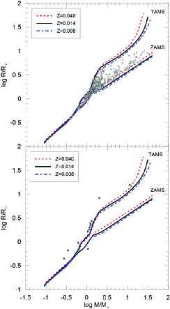
Figure 1: a) Positions of 400 stars (194 binaries, eight primary and four secondary), b) positions of discarded components (eight secondary, four primary) on the $M-R$ diagram. ZAMS and TAMS lines of PARSEC stellar evolution models (dash-dot $Z=0.008$, solid Solar, dotted $Z$=0.040) mark the region of the main-sequence stars.

2.4 Propagation of observational uncertainties to $BC$

According to Eq. (1) there are two groups of observational uncertainties to be propagated. The first group propagates trough $M_{Bol}$ and the other group propagates trough $M_{V}$. Therefore, according to Eq. (1), we can write for an uncertainty of a $BC$,

$$\Delta BC=\sqrt{(\Delta M_{Bol})^{2}+(\Delta M_{V})^{2}}.$$ (7)

Eqs. (2) and (4) indicates that the first group of uncertainties is included in

$$\Delta M_{Bol}=2.5\log e\sqrt{\left(2\frac{\Delta R}{R}\right)^{2}+\left(4\frac{\Delta T}{T}\right)^{2}.}$$ (8)

Since radius ($R_{\odot}$) and effective temperature ($T_{eff,\odot}$) of the Sun are just constants, Eq. (8) assumes no uncertainty contribution from them. The contributions are from the relative uncertainties of radii and effective temperatures of the stars in concern. Relative uncertainty of temperature usually dominates because relative errors of temperatures are usually bigger than relative errors of radii and a temperature uncertainty contributes two times even if the relative uncertainties are the same because of the power of the temperature is twice of the power of radius as appeared in the Stefan-Boltzmann law.

According to Eq. (5), the second group of uncertainties is included in

$$\Delta M_{V}=\sqrt{\left(\Delta m_{V}\right)^{2}+\left(5\log e\frac{\sigma_{\varpi}}{\varpi}\right)^{2}+\left(\Delta A_{V}\right)^{2}.}$$ (9)

Basically, there are three kinds of observational uncertainties that determine the uncertainty of $M_{V}$: Uncertainty of the $V$ magnitude of the component ($\Delta m_{V}$), uncertainty of interstellar extinction ($\Delta A_{V}$) and the uncertainty of the distance ($\sigma_{\varpi}/\varpi$). Because, the relative uncertainty of a distance is same as the relative uncertainty of the parallax, and the relative uncertainties of trigonometric parallaxes are given in Table 1, the relative uncertainty of a trigonometric parallax is entered in Eq. (9). The coefficient $5\log e=2.1715$ is inevitable because of Eq. (5). For simplicity, we have assumed that $V$ magnitude uncertainties of the components are the same as the $V$ magnitude uncertainty of the system. This is a reasonable assumption because considerable number of systems given light ratio ($L_{2}/L_{1}$) in this study is found without uncertainties. However, systemic brightness uncertainties are already in Table 1. Since both $\Delta m_{V}$ and $\Delta A_{V}$ are usually about $\pm 0.01$ or smaller, trigonometric parallax uncertainties dominates. Not only this but also because of $5\log e=2.1715$ values, the weight of parallax contributions to $\Delta M_{V}$ are approximately doubled.

The distribution of Gaia relative parallax errors for the systems in our list are shown in Fig. 2. It has been known that if parallax precisions worse than 10%, the error distribution in parallaxes creates a bias in Gaia distances (Bailer-Jones & Coryn, 2015; Bailer-Jones et al., 2018). Since 95% of distances in this study have relative parallax errors less than nine per cent, the distances used in this study apparently are not affected from the bias.

Figure 2: Cumulative (above) and histogram (below) distributions of relative parallax errors of Gaia distances.

3 Results

3.1 Determination of missing light ratios ($L_{2}/L_{1}$)

The light ratio ($L_{2}/L_{1}$) is an essential parameter to obtain component apparent brightness’ from the apparent brightness of the system. It can be seen in the right most columns Table 1 that there exist 47 systems, which are given references to Graczyk et al. (2019) from whom light ratios in $B$ and $V$ bands are taken. Associated to 33 stars, the next most popular reference for the light ratios is “this study”, which implies the light ratio (or ratios) is obtained by solving eclipsing light curve of the system. If these two references are absent, the number of systems would have reduced from 206 to 126. That is, statistical reliability of current results would have been greatly (almost 50%) reduced.

We went through original references of 550 stars collected in the first step and collected primarily the light ratio ($L_{2}/L_{1}$) in the $V$ band, and if exist in the $B$ band. We faced up the reality that not all simultaneous LC and RV solutions of detached double lined spectroscopic binaries are done in the Johnson photometry. There is great deal of systems that their solutions are done in the Strömgren photometry and some of the other systems like Kepler photometry, which are lost automatically because we are interested in only the light ratios in the $V$ band. Moreover, we run into publications such that the light ratio of a system is obtained but it is not given. Only physical parameters and/or other light curve solutions are given. Some of such publications do not even give brightness of the system which is also needed.

Aiming to keep the loss of systems at a minimum level, we have requested $L_{2}/L_{1}$ from considerable number authors by private communications. V781 Per, VZ Cep, AP And (Zola et al., 2014), GJ 3236 (Irwin et al., 2006), V1236 Tau (Bayless & Orosz,, 2006), V404 CMa (Rozyczka et al., 2009), Corot 102932176 (Lazaro, Arevalo & Almenara, 2015), UV Leo (Kjurkchieva & Marchev, 2007), EM Car (Çiçek, Bulut & Bulut, 2017), eta Mus, GG Lup (Budding, Butland & Blackford, 2015, 2017), EK Cep (Antonyuk & Rostopchina, 2009) and BW Aqr (Volkov & Chochol, 2007) are the systems which we have requested $L_{2}/L_{1}$ information, if available. If not, at least $V$ and/or $B$ data are asked and got a positive reply. V1200 Cen, GU Boo, and OO Peg are the systems we did not get any reply.

Some systems in our list contained the $V$ data printed in the paper itself or in public ASAS data archive. All those systems, which we could not find $L_{2}/L_{1}$, but got their data, are solved in this study using Wilson Devinney code (Wilson & van Hamme, 2014) in common way (e.g. Bakış, Yücel & Bakış, 2018; Soydugan et al., 2013). Since the light and radial velocity curves of all these 33 systems were already analyzed in literature, the effective temperature of the primary ($T_{1}$) and the mass ratios of the system ($q$) were adopted from Table 2 and kept fixed during the analysis. The bolometric albedo, gravitational and limb darkening coefficients of the components were used in the same way as the values used in the analyses given in the literature. The third light contribution was also tested during the analysis. Light curves were solved in Mode 2, which corresponds to detached binaries in Wilson-Devinney code. The final parameters are given in Table 3, where the columns are self explanatory: ID number, name of the system, orbital period, temperature of primary, temperature of secondary, mass ratio, fractional radius of primary and secondary, light ratio in $V$-band, third light in $V$, light ratio in $B$-band, third light in $B$ and reference.

Table 3: Light ratios ($L_{2}/L_{1}$) from simultaneous light and radial curves analysis of 33 detached binaries that do not have light ratio information in their literature.

								in $V$ filter		in $B$ filter
ID	System	$P$	$T_{1}$	$T_{2}$	$q$	$r_{1}$	$r_{2}$	$L_{2}/L_{1}$	$L_{3}$	$L_{2}/L_{1}$	$L_{3}$	Reference
		(days)	(K)	(K)	($M_{2}/M_{1}$)	($R_{1}/a$)	($R_{2}/a$)		(%)		(%)
1	2MASS J01132817-3821024	0.445596	3750	3112$\pm$200	0.727	0.2380$\pm$0.0002	0.1780$\pm$0.0002	0.131$\pm$0.020	—	—	—	ASAS
2	V505 Per	4.22202	6512	6462$\pm$201	0.986	0.0861$\pm$0.0001	0.0847$\pm$0.0001	0.951$\pm$0.010	—	0.93$\pm$0.01	—	Tomasella et al. (2008)
3	TYC 4749-560-1	1.622219	5340	5125$\pm$200	0.993	0.1233$\pm$0.0005	0.1211$\pm$0.0005	0.993$\pm$0.010	—	—	—	Hełminiak & Konacki (2011)
4	V1236 Tau	2.58791	4200	4133$\pm$250	0.978	0.0829$\pm$0.0010	0.0869$\pm$0.0005	1.039$\pm$0.010	—	—	—	Bayless & Orosz, (2006)
5	V432 Aur	3.081745	6080	6685$\pm$85	0.883	0.2097$\pm$0.0002	0.1049$\pm$0.0002	0.372$\pm$0.020	—	0.43$\pm$0.02	—	Siviero et al. (2004)
6	V1388 Ori	2.18706	20500	18900$\pm$500	0.695	0.3400$\pm$0.0004	0.2283$\pm$0.0004	0.344$\pm$0.008	—	—	—	ASAS
7	V404 CMa	0.45178	4200	3940$\pm$20	0.879	0.2603$\pm$0.0001	0.2462$\pm$0.0001	0.620$\pm$0.010	—	0.55$\pm$0.01	—	Rozyczka et al. (2009)
8	CoRoT 102932176	0.872241	7300	4547$\pm$80	0.405	0.3253$\pm$0.0001	0.1457$\pm$0.0001	0.027$\pm$0.012	—	—	—	Lazaro et al. (2015)
9	HI Mon	1.57443	30000	29000$\pm$682	0.863	0.2815$\pm$0.0002	0.2739$\pm$0.0002	0.937$\pm$0.020	7$\pm$2	—	—	ASAS
10	TYC 176-2950-1	11.55478	5735	5733$\pm$200	0.986	0.0601$\pm$0.0001	0.0430$\pm$0.0001	0.511$\pm$0.011	—	—	—	ASAS
11	CW CMa	2.117977	9886	9639$\pm$200	1.058	0.1734$\pm$0.0002	0.1642$\pm$0.0002	0.994$\pm$0.013	—	—	—	ASAS
12	ASAS-08	1.528489	4350	4310$\pm$205	0.978	0.1114$\pm$0.0001	0.1122$\pm$0.0001	0.944$\pm$0.020	—	—	—	ASAS
13	ASAS-09	0.89742	4360	4360$\pm$150	1.004	0.1701$\pm$0.0002	0.1695$\pm$0.0002	0.993$\pm$0.012	—	—	—	ASAS
14	DU Leo	1.374185	5940	5788$\pm$130	0.983	0.1916$\pm$0.0002	0.1969$\pm$0.0002	0.950$\pm$0.010	—	—	—	ASAS
15	QX Car	4.47804	23800	22600$\pm$500	0.915	0.1442$\pm$0.0001	0.1361$\pm$0.0001	0.815$\pm$0.010	—	0.81$\pm$0.01	—	Cousins (1981)
16	HS Hya	1.568041	6500	6329$\pm$50	0.971	0.1668$\pm$0.0001	0.1593$\pm$0.0001	0.818$\pm$0.010	—	—	—	ASAS
17	UW LMi	3.874307	6500	6528$\pm$205	1.017	0.0956$\pm$0.0001	0.0940$\pm$0.0001	0.996$\pm$0.010	—	—	—	Hipparcos
18	eta Mus	2.396316	12700	12550$\pm$300	0.999	0.1517$\pm$0.0001	0.1510$\pm$0.0002	0.960$\pm$0.008	—	0.93$\pm$0.01	—	Bakış et al. (2007)
19	V1200 Cen	2.4828778	6266	4706$\pm$205	0.621	0.1372$\pm$0.0002	0.1086$\pm$0.0001	0.168$\pm$0.003	—	—	—	ASAS
20	TV Nor	8.524391	9120	7916$\pm$201	0.811	0.0685$\pm$0.0002	0.0578$\pm$0.0002	0.452$\pm$0.003	—	0.49$\pm$0.01	—	North et al. (1997)
21	HD147827	8.87621	5957	5811$\pm$230	0.852	0.1100$\pm$0.0010	0.0830$\pm$0.0006	0.521$\pm$0.008	—	—	—	ASAS
22	FL Lyr	2.178154	6150	5200$\pm$202	0.786	0.1398$\pm$0.0002	0.1049$\pm$0.0001	0.249$\pm$0.016	—	—	—	Popper (1986)
23	WOCS 24009	3.649303	5925	5860$\pm$201	0.987	0.0852$\pm$0.0001	0.0829$\pm$0.0001	0.975$\pm$0.011	61.63$\pm$1.50	—	—	Kepler
24	WOCS 40007	3.185096	6350	5930$\pm$150	0.875	0.1164$\pm$0.0002	0.0913$\pm$0.0002	0.505$\pm$0.013	0.43$\pm$0.03	0.48$\pm$0.01	0.18$\pm$0.04	Jeffries et al. (2013)
25	BD-20 5728	7.04335	5957	5943$\pm$205	0.721	0.1253$\pm$0.0002	0.0929$\pm$0.0002	0.542$\pm$0.017	—	—	—	ASAS
26	MT91 372	2.227582	24000	15616$\pm$200	0.440	0.2600$\pm$0.0003	0.1758$\pm$0.0003	0.210$\pm$0.022	—	—	—	Kiminki et al. (2015)
27	MT91 696	1.469179	32000	30910$\pm$1050	0.800	0.3902$\pm$0.0002	0.3509$\pm$0.0002	0.739$\pm$0.014	—	—	—	Kiminki et al. (2015)
28	ASAS-21	0.70243	4750	4220$\pm$180	0.851	0.2206$\pm$0.0001	0.1875$\pm$0.0001	0.418$\pm$0.012	—	—	—	ASAS
29	EK Cep	4.427822	9000	5700$\pm$190	0.554	0.0949$\pm$0.0001	0.0791$\pm$0.0001	0.126$\pm$0.013	—	0.09$\pm$0.02	—	Antonyuk & Rostopchina (2009)
30	OO Peg	2.985	7850	7600$\pm$450	0.983	0.1648$\pm$0.0002	0.1462$\pm$0.0002	0.698$\pm$0.013	—	—	—	ASAS
31	NGC 7142 V2	15.6506	6238	6276$\pm$63	1.000	0.0438$\pm$0.0001	0.0437$\pm$0.0001	1.004$\pm$0.013	—	1.02$\pm$0.01	—	Sandquist et al. (2013)
32	BG Ind	1.464069	6353	6718$\pm$233	0.894	0.3073$\pm$0.0002	0.2254$\pm$0.0002	0.469$\pm$0.006	—	—	—	ASAS
33	V453 Cep	1.184725	10300	10410$\pm$500	0.962	0.2627$\pm$0.0002	0.2501$\pm$0.0002	1.063$\pm$0.005	—	—	—	Griffin & Griffin (2009)

3.2 $BC$ coefficients

The $BC$ coefficients computed from the parameters of 400 main-sequence stars (206 binaries) with metallicities $0.008\leq Z\leq 0.040$ in the Solar neighborhood are listed in Table 4. The columns of Table 4 are organized as: ID number, name of the system, $(B-V)_{0}$ for primary, $(B-V)_{0}$ for secondary, bolometric magnitude and its error for the primary, bolometric magnitude and its error for the secondary, $BC$ and its error for the primary, $BC$ and its error for the secondary. Notice that $BC$ values and associated uncertainties are not given for one of the components of the 12 systems, which are not on the main-sequence (Fig. 1b). Only bolometric absolute magnitudes are given for interested readers, who may want to calculate visual absolute magnitudes either using $BC$ values according to Eq. (1) or according to Eq. (5).

Table 4: De-reddened colours, bolometric magnitudes and bolometric correction coefficients of the present sample.

ID	Name	Pri $(B-V)_{0}$	Sec $(B-V)_{0}$	Pri $M_{Bol}$	Sec $M_{Bol}$	Pri $BC$	Sec $BC$
		(mag)	(mag)	(mag)	(mag)	(mag)	(mag)
1	V421 Peg	—	—	2.751$\pm$0.061	3.299$\pm$0.088	0.093$\pm$0.065	0.090$\pm$0.091
2	DV Psc	0.943	1.311	6.691$\pm$0.095	8.219$\pm$0.085	-0.906$\pm$0.096	-1.633$\pm$0.086
3	MU Cas	-0.097	-0.101	-2.447$\pm$0.149	-2.260$\pm$0.146	-0.921$\pm$0.244	-0.983$\pm$0.241
4	GSC 4019-3345	0.114	0.118	1.781$\pm$0.168	1.781$\pm$0.294	-0.142$\pm$0.209	-0.125$\pm$0.319
5	YZ Cas	-0.035	0.363	0.556$\pm$0.056	3.356$\pm$0.152	-0.101$\pm$0.061	0.061$\pm$0.154
6	NGC188 KR V12	—	—	3.876$\pm$0.079	3.973$\pm$0.080	0.178$\pm$0.117	0.177$\pm$0.118
7	V364 Cas	0.174	0.276	1.951$\pm$0.049	1.608$\pm$0.049	-0.184$\pm$0.108	-0.195$\pm$0.108
8	zet Phe	-0.111	-0.073	-1.552$\pm$0.106	0.254$\pm$0.077	-1.005$\pm$0.131	-0.542$\pm$0.109
9	CO And	—	—	3.285$\pm$0.096	3.306$\pm$0.094	-0.035$\pm$0.111	-0.031$\pm$0.109
10	V459 Cas	0.070	0.076	1.228$\pm$0.143	1.295$\pm$0.144	-0.094$\pm$0.165	-0.093$\pm$0.165
11	2MASS J01132817-3821024	—	—	7.737$\pm$0.299	9.181$\pm$0.303	-1.204$\pm$0.299	-1.967$\pm$0.303
12	UV Psc	0.652	1.062	4.494$\pm$0.085	5.978$\pm$0.107	-0.366$\pm$0.086	-0.767$\pm$0.108
13	NSVS 06507557	—	—	7.475$\pm$0.139	—	-0.527$\pm$0.139	—
14	AL Ari	0.428	0.690	3.672$\pm$0.056	5.246$\pm$0.065	0.167$\pm$0.068	0.048$\pm$0.076
15	V615 Per	-0.163	-0.075	-1.209$\pm$0.197	0.541$\pm$0.225	-1.304$\pm$0.298	-0.193$\pm$0.317
16	V505 Per	0.396	0.425	3.667$\pm$0.136	3.736$\pm$0.137	0.075$\pm$0.137	0.090$\pm$0.138
17	DN Cas	-0.208	-0.203	-7.004$\pm$0.136	-5.935$\pm$0.172	-3.535$\pm$0.201	-3.171$\pm$0.226
18	AG Ari	0.006	0.037	0.481$\pm$0.108	0.857$\pm$0.104	-0.150$\pm$0.126	-0.045$\pm$0.123
19	XY Cet	0.179	0.231	2.027$\pm$0.075	2.286$\pm$0.080	0.229$\pm$0.089	0.195$\pm$0.093
20	CW Eri	0.314	0.379	2.399$\pm$0.075	3.205$\pm$0.117	0.006$\pm$0.079	0.019$\pm$0.120
21	V799 Cas	-0.092	-0.084	-0.819$\pm$0.094	-0.669$\pm$0.095	-0.546$\pm$0.120	-0.482$\pm$0.121
22	AE For	1.327	1.349	7.095$\pm$0.097	7.277$\pm$0.104	-1.276$\pm$0.099	-1.308$\pm$0.106
23	V570 Per	0.377	0.438	3.130$\pm$0.161	3.513$\pm$0.182	0.049$\pm$0.162	0.037$\pm$0.184
24	IM Per	—	—	1.647$\pm$0.087	1.692$\pm$0.093	0.266$\pm$0.117	0.263$\pm$0.121
25	TV Cet	0.346	0.414	3.106$\pm$0.099	3.741$\pm$0.101	0.049$\pm$0.101	0.025$\pm$0.103
26	TZ For	0.488	—	1.329$\pm$0.084	—	-0.074$\pm$0.086	—
27	GJ 3236	—	—	9.239$\pm$0.148	9.988$\pm$0.148	-2.537$\pm$0.157	-2.511$\pm$0.156
28	EY Cep	0.315	0.336	3.021$\pm$0.093	3.087$\pm$0.095	0.009$\pm$0.097	0.013$\pm$0.099
29	V1229 Tau	-0.064	0.212	1.189$\pm$0.135	2.638$\pm$0.183	-0.032$\pm$0.140	0.243$\pm$0.186
30	IQ Per	-0.105	0.178	-0.505$\pm$0.075	2.612$\pm$0.064	-0.491$\pm$0.089	0.295$\pm$0.079
31	SZ Cam	-0.226	-0.195	-7.333$\pm$0.038	-5.902$\pm$0.058	-3.052$\pm$0.219	-2.557$\pm$0.223
32	V1094 Tau	0.684	0.724	3.934$\pm$0.075	4.575$\pm$0.077	-0.056$\pm$0.091	-0.060$\pm$0.094
33	NP Per	—	—	3.591$\pm$0.064	5.335$\pm$0.155	-0.033$\pm$0.087	-0.457$\pm$0.166
34	V818 Tau	0.710	1.193	5.207$\pm$0.457	6.934$\pm$0.281	0.122$\pm$0.458	-0.444$\pm$0.282
35	AL Dor	0.568	0.556	4.374$\pm$0.082	4.339$\pm$0.082	-0.016$\pm$0.084	-0.011$\pm$0.084
36	TYC 4749-560-1	—	—	5.436$\pm$0.163	5.653$\pm$0.170	-0.289$\pm$0.207	-0.149$\pm$0.213
37	HP Aur	—	—	4.652$\pm$0.090	5.778$\pm$0.101	-0.210$\pm$0.097	-0.327$\pm$0.108
38	V1236 Tau	—	—	6.700$\pm$0.211	6.667$\pm$0.264	-0.461$\pm$0.441	-0.453$\pm$0.469
39	CD Tau	0.433	0.436	3.155$\pm$0.041	3.431$\pm$0.044	0.174$\pm$0.044	0.169$\pm$0.047
40	AR Aur	-0.073	-0.040	0.654$\pm$0.120	0.915$\pm$0.126	-0.228$\pm$0.124	-0.138$\pm$0.130
41	EW Ori	—	—	4.182$\pm$0.069	4.442$\pm$0.071	-0.010$\pm$0.074	-0.070$\pm$0.076
42	AS Cam	—	—	-0.528$\pm$0.220	0.562$\pm$0.216	-0.608$\pm$0.232	-0.515$\pm$0.228
43	UX Men	0.500	0.551	3.779$\pm$0.073	3.937$\pm$0.074	0.013$\pm$0.075	0.022$\pm$0.076
44	TZ Men	-0.114	0.258	0.659$\pm$0.210	2.999$\pm$0.182	-0.287$\pm$0.219	0.076$\pm$0.192
45	V432 Aur	—	0.389	—	3.649$\pm$0.012	—	-0.164$\pm$0.026
46	GG Ori	-0.048	-0.053	1.037$\pm$0.092	1.063$\pm$0.092	0.025$\pm$0.159	0.029$\pm$0.159
47	beta Aur	0.044	0.012	0.439$\pm$0.094	0.667$\pm$0.095	-0.173$\pm$0.095	-0.009$\pm$0.096
48	V530 Ori	0.583	1.337	4.696$\pm$0.079	7.621$\pm$0.137	-0.021$\pm$0.083	-1.061$\pm$0.139
49	V1388 Ori	—	—	-4.507$\pm$0.107	-3.289$\pm$0.116	-2.214$\pm$0.366	-2.154$\pm$0.369
50	FT Ori	0.006	0.117	1.170$\pm$0.182	1.953$\pm$0.152	-0.074$\pm$0.193	0.052$\pm$0.166
51	V404 CMa	0.877	1.005	6.831$\pm$0.112	7.229$\pm$0.058	-0.467$\pm$0.232	-0.587$\pm$0.212
52	IM Mon	-0.212	-0.176	-2.569$\pm$0.091	-1.126$\pm$0.167	-1.373$\pm$0.116	-0.814$\pm$0.182
53	RR Lyn	0.193	0.260	1.524$\pm$0.060	2.919$\pm$0.075	0.136$\pm$0.115	0.135$\pm$0.123
54	KL CMa	—	—	-0.726$\pm$0.089	0.320$\pm$0.248	-0.313$\pm$0.110	-0.403$\pm$0.257
55	V578 Mon	-0.240	-0.210	-6.084$\pm$0.074	-4.917$\pm$0.078	-2.440$\pm$0.715	-2.107$\pm$0.715
56	WW Aur	0.143	0.163	1.919$\pm$0.229	2.179$\pm$0.233	0.064$\pm$0.238	0.066$\pm$0.241
57	TYC 7091-888-1	—	0.734	—	5.716$\pm$0.069	—	-0.133$\pm$0.082
58	V501 Mon	0.183	0.276	2.217$\pm$0.067	2.893$\pm$0.068	0.099$\pm$0.125	0.109$\pm$0.125
59	GX Gem	0.509	0.521	2.593$\pm$0.071	2.698$\pm$0.071	0.250$\pm$0.137	0.234$\pm$0.138
60	CoRoT 102932176	—	—	2.659$\pm$0.073	6.459$\pm$0.097	0.009$\pm$0.154	-0.099$\pm$0.166
61	HS Aur	—	—	5.059$\pm$0.075	5.486$\pm$0.096	0.084$\pm$0.077	0.052$\pm$0.097
62	HI Mon	—	—	-5.813$\pm$0.086	-5.606$\pm$0.107	-2.738$\pm$0.525	-2.601$\pm$0.529
63	LT CMa	—	—	-2.733$\pm$0.135	-0.387$\pm$0.270	-1.558$\pm$0.161	-0.857$\pm$0.284
64	SW CMa	0.139	0.148	0.819$\pm$0.081	1.282$\pm$0.088	0.270$\pm$0.107	0.306$\pm$0.113
65	GZ CMa	0.073	0.111	0.923$\pm$0.175	1.401$\pm$0.178	-0.066$\pm$0.178	-0.019$\pm$0.182
66	TYC 176-2950-1	—	—	—	4.406$\pm$0.156	—	0.093$\pm$0.163
67	CW CMa	—	—	1.002$\pm$0.099	1.231$\pm$0.124	-0.451$\pm$0.105	-0.229$\pm$0.129
68	FS Mon	0.362	0.395	2.512$\pm$0.066	3.121$\pm$0.068	0.049$\pm$0.073	0.032$\pm$0.075
69	YY Gem	—	—	7.567$\pm$0.116	7.624$\pm$0.116	-1.547$\pm$0.116	-1.508$\pm$0.116
70	V392 Car	—	—	1.831$\pm$0.106	1.963$\pm$0.109	0.117$\pm$0.113	0.131$\pm$0.115
71	AI Hya	—	—	1.633$\pm$0.040	1.131$\pm$0.042	0.445$\pm$0.098	0.321$\pm$0.099
72	ASAS-08	—	—	6.762$\pm$0.207	6.786$\pm$0.210	-1.349$\pm$0.218	-1.387$\pm$0.222
73	AY Cam	0.398	0.381	1.527$\pm$0.062	2.122$\pm$0.061	0.051$\pm$0.068	0.040$\pm$0.067
74	HD 71636	0.389	0.501	2.946$\pm$0.088	3.589$\pm$0.095	0.054$\pm$0.090	0.036$\pm$0.097
75	CU Cnc	—	—	9.174$\pm$0.208	9.438$\pm$0.214	-2.201$\pm$0.208	-2.293$\pm$0.215

Table 5: continued

ID	Name	Pri $(B-V)_{0}$	Sec $(B-V)_{0}$	Pri $M_{Bol}$	Sec $M_{Bol}$	Pri $BC$	Sec $BC$
		(mag)	(mag)	(mag)	(mag)	(mag)	(mag)
76	VZ Hya	0.423	0.508	3.534$\pm$0.098	4.134$\pm$0.104	-0.025$\pm$0.103	-0.038$\pm$0.109
77	KX Cnc	0.563	0.578	4.401$\pm$0.079	4.471$\pm$0.080	-0.017$\pm$0.081	-0.022$\pm$0.082
78	RS Cha	0.182	0.186	1.861$\pm$0.074	1.899$\pm$0.070	0.120$\pm$0.076	0.174$\pm$0.071
79	V467 Vel	-0.344	-0.299	-8.232$\pm$0.022	-4.385$\pm$0.023	-2.946$\pm$0.510	-2.126$\pm$0.511
80	NSVS 02502726	0.998	—	6.777$\pm$0.203	—	-0.351$\pm$0.204	—
81	EPIC 211409263	0.565	—	4.351$\pm$0.073	—	0.134$\pm$0.091	—
82	CV Vel	-0.198	-0.196	-3.253$\pm$0.122	-3.124$\pm$0.123	-1.466$\pm$0.133	-1.389$\pm$0.134
83	XY UMa	0.753	0.957	4.869$\pm$0.038	7.202$\pm$0.035	-0.517$\pm$0.039	-1.050$\pm$0.037
84	PT Vel	-0.084	0.145	1.087$\pm$0.073	2.558$\pm$0.106	0.044$\pm$0.166	0.190$\pm$0.182
85	KW Hya	0.234	0.432	1.681$\pm$0.110	3.105$\pm$0.130	0.014$\pm$0.112	0.015$\pm$0.132
86	ASAS-09	—	—	6.529$\pm$0.153	6.537$\pm$0.154	-0.448$\pm$0.382	-0.447$\pm$0.383
87	DU Leo	—	—	4.252$\pm$0.092	4.365$\pm$0.112	0.058$\pm$0.093	0.114$\pm$0.114
88	QX Car	-0.224	-0.218	-4.576$\pm$0.096	-4.227$\pm$0.101	-2.340$\pm$0.138	-2.213$\pm$0.142
89	HS Hya	—	—	3.691$\pm$0.035	3.908$\pm$0.037	0.126$\pm$0.041	0.125$\pm$0.042
90	UV Leo	0.597	0.623	4.573$\pm$0.072	4.373$\pm$0.088	-0.220$\pm$0.073	-0.276$\pm$0.089
91	RZ Cha	0.395	0.406	2.461$\pm$0.109	2.461$\pm$0.109	-0.078$\pm$0.111	0.025$\pm$0.111
92	DW Car	-0.213	-0.208	-5.398$\pm$0.157	-5.046$\pm$0.166	-2.148$\pm$0.281	-1.987$\pm$0.286
93	UW LMi	—	—	3.707$\pm$0.163	3.724$\pm$0.174	-0.223$\pm$0.164	-0.210$\pm$0.175
94	EM Car	-0.255	-0.256	-7.817$\pm$0.258	-7.569$\pm$0.259	-2.709$\pm$0.416	-2.709$\pm$0.416
95	FM Leo	0.463	0.498	3.263$\pm$0.174	3.539$\pm$0.163	0.106$\pm$0.177	0.095$\pm$0.166
96	MW UMa	—	—	3.716$\pm$0.088	4.211$\pm$0.025	-0.142$\pm$0.092	-0.051$\pm$0.036
97	EP Cru	-0.158	-0.152	-2.381$\pm$0.140	-2.239$\pm$0.143	-1.110$\pm$0.178	-1.083$\pm$0.181
98	VV Crv	0.423	0.413	1.583$\pm$0.134	3.045$\pm$0.131	0.100$\pm$0.135	0.093$\pm$0.132
99	IM Vir	0.621	1.106	4.764$\pm$0.085	6.904$\pm$0.139	-0.249$\pm$0.086	-0.921$\pm$0.140
100	HY Vir	0.384	0.459	1.734$\pm$0.079	3.265$\pm$0.080	-0.010$\pm$0.086	-0.034$\pm$0.087
101	eta Mus	-0.132	-0.089	-0.337$\pm$0.040	-0.275$\pm$0.112	-0.388$\pm$0.063	-0.371$\pm$0.122
102	SZ Cen	0.120	0.147	0.666$\pm$0.113	0.297$\pm$0.116	0.151$\pm$0.126	0.159$\pm$0.128
103	V1200 Cen	—	—	3.668$\pm$0.274	5.420$\pm$0.529	0.125$\pm$0.276	-0.062$\pm$0.530
104	ZZ Boo	0.373	0.329	2.314$\pm$0.071	2.270$\pm$0.071	-0.046$\pm$0.073	-0.090$\pm$0.073
105	BH Vir	0.467	0.555	4.054$\pm$0.114	4.707$\pm$0.176	-0.139$\pm$0.118	-0.169$\pm$0.179
106	DM Vir	0.469	0.469	2.992$\pm$0.070	2.992$\pm$0.202	-0.002$\pm$0.076	-0.002$\pm$0.204
107	AD Boo	0.377	0.486	3.135$\pm$0.081	4.040$\pm$0.087	-0.014$\pm$0.093	-0.097$\pm$0.097
108	GG Lup	-0.149	-0.076	-0.705$\pm$0.110	0.836$\pm$0.132	-0.726$\pm$0.123	-0.408$\pm$0.143
109	AQ Ser	—	—	2.481$\pm$0.069	2.386$\pm$0.073	0.152$\pm$0.087	0.149$\pm$0.090
110	CV Boo	—	—	4.232$\pm$0.120	4.458$\pm$0.122	-0.173$\pm$0.137	-0.055$\pm$0.140
111	V335 Ser	0.049	0.088	1.026$\pm$0.134	1.843$\pm$0.122	-0.167$\pm$0.136	-0.095$\pm$0.125
112	TV Nor	0.062	-0.029	1.416$\pm$0.072	2.403$\pm$0.112	-0.049$\pm$0.084	0.075$\pm$0.120
113	V760 Sco	-0.164	-0.155	-2.331$\pm$0.136	-1.890$\pm$0.139	-1.467$\pm$0.151	-1.378$\pm$0.154
114	HD147827	—	—	2.569$\pm$0.318	—	0.151$\pm$0.321	—
115	V349 Ara	—	—	-0.006$\pm$0.105	0.135$\pm$0.113	-0.177$\pm$0.124	-0.005$\pm$0.131
116	V923 Sco	0.334	0.367	2.535$\pm$0.064	2.826$\pm$0.066	0.099$\pm$0.066	0.083$\pm$0.067
117	V2626 Oph	0.329	0.482	0.903$\pm$0.065	3.226$\pm$0.068	-0.033$\pm$0.073	-0.096$\pm$0.075
118	WZ Oph	0.503	0.509	3.722$\pm$0.073	3.729$\pm$0.073	-0.082$\pm$0.078	-0.062$\pm$0.078
119	V2365 Oph	0.021	0.532	0.873$\pm$0.092	4.440$\pm$0.143	-0.324$\pm$0.113	-0.179$\pm$0.157
120	V2368 Oph	0.114	0.103	-0.263$\pm$0.094	-0.288$\pm$0.092	-0.231$\pm$0.099	-0.269$\pm$0.097
121	U Oph	-0.248	-0.164	-2.481$\pm$0.387	-2.050$\pm$0.409	-1.800$\pm$0.471	-1.595$\pm$0.489
122	TX Her	0.222	0.317	2.446$\pm$0.122	3.333$\pm$0.145	0.098$\pm$0.123	0.180$\pm$0.146
123	LV Her	0.573	0.581	3.864$\pm$0.109	3.959$\pm$0.110	0.029$\pm$0.128	0.028$\pm$0.128
124	V501 Her	0.719	0.703	3.301$\pm$0.076	3.883$\pm$0.076	-0.032$\pm$0.093	-0.015$\pm$0.092
125	V624 Her	—	—	0.836$\pm$0.083	1.632$\pm$0.087	0.103$\pm$0.085	0.107$\pm$0.089
126	BD-00 3357	—	—	2.498$\pm$0.245	3.672$\pm$0.117	0.160$\pm$0.252	-0.124$\pm$0.131
127	V539 Ara	-0.133	-0.264	-3.482$\pm$0.316	-2.808$\pm$0.343	-1.994$\pm$0.443	-1.963$\pm$0.463
128	V2653 Oph	—	—	2.207$\pm$0.305	2.820$\pm$0.449	-0.318$\pm$0.394	-0.282$\pm$0.514
129	Z Her	0.338	—	2.947$\pm$0.087	—	0.020$\pm$0.087	—
130	V994 Her-B	0.008	0.095	1.813$\pm$0.163	2.214$\pm$0.122	-0.309$\pm$0.443	-0.106$\pm$0.430
131	V994 Her-A	-0.080	0.000	-0.073$\pm$0.103	1.462$\pm$0.065	-0.698$\pm$0.425	-0.200$\pm$0.417
132	V451 Oph	-0.122	-0.070	-0.094$\pm$0.323	0.901$\pm$0.224	-0.561$\pm$0.329	-0.336$\pm$0.233
133	RX Her	—	—	-0.053$\pm$0.102	0.843$\pm$0.125	-0.884$\pm$0.106	-0.538$\pm$0.128
134	V413 Ser	—	—	-0.626$\pm$0.122	-0.124$\pm$0.123	-0.346$\pm$0.588	-0.075$\pm$0.588
135	QY Tel	—	—	2.988$\pm$0.229	2.207$\pm$0.189	-0.235$\pm$0.237	-0.220$\pm$0.199
136	V4403 Sgr	—	—	3.010$\pm$0.103	2.359$\pm$0.107	0.008$\pm$0.107	0.034$\pm$0.110
137	V1331 Aql	-0.255	-0.184	-4.839$\pm$0.023	-3.712$\pm$0.034	-2.568$\pm$0.086	-2.048$\pm$0.090
138	YY Sgr	-0.154	-0.141	-1.404$\pm$0.207	-0.996$\pm$0.211	-0.973$\pm$0.254	-0.880$\pm$0.257
139	DI Her	-0.180	-0.153	-2.086$\pm$0.209	-1.418$\pm$0.210	-1.270$\pm$0.216	-0.979$\pm$0.217
140	HP Dra	0.462	0.719	3.936$\pm$0.110	4.588$\pm$0.113	-0.083$\pm$0.111	-0.105$\pm$0.113
141	V1182 Aql	-0.292	-0.243	-8.753$\pm$0.067	-5.923$\pm$0.107	-4.378$\pm$0.162	-3.340$\pm$0.183
142	V1665 Aql	-0.097	-0.074	-1.626$\pm$0.134	-0.386$\pm$0.126	-0.860$\pm$0.149	-0.728$\pm$0.141
143	V805 Aql	0.152	0.326	1.589$\pm$0.214	2.566$\pm$0.235	-0.210$\pm$0.216	-0.138$\pm$0.236
144	FL Lyr	—	—	3.925$\pm$0.151	5.277$\pm$0.182	0.019$\pm$0.153	-0.139$\pm$0.183
145	V565 Lyr	—	—	4.662$\pm$0.075	5.069$\pm$0.102	0.159$\pm$0.993	0.072$\pm$0.996
146	V1430 Aql	0.790	0.695	4.933$\pm$0.125	5.775$\pm$0.092	-0.128$\pm$0.128	-0.154$\pm$0.095
147	UZ Dra	0.444	0.499	3.834$\pm$0.092	4.279$\pm$0.088	0.114$\pm$0.094	0.068$\pm$0.091
148	V2080 Cyg	0.500	0.505	3.557$\pm$0.055	3.562$\pm$0.055	0.067$\pm$0.057	0.068$\pm$0.057
149	V2083 Cyg	0.223	0.216	1.726$\pm$0.176	1.416$\pm$0.179	0.346$\pm$0.336	0.320$\pm$0.338
150	V885 Cyg	—	—	1.145$\pm$0.079	0.466$\pm$0.082	0.163$\pm$0.109	0.175$\pm$0.112

Table 5: continued

ID	Name	Pri $(B-V)_{0}$	Sec $(B-V)_{0}$	Pri $M_{Bol}$	Sec $M_{Bol}$	Pri $BC$	Sec $BC$
		(mag)	(mag)	(mag)	(mag)	(mag)	(mag)
151	V4089 Sgr	0.029	0.243	0.106$\pm$0.052	2.657$\pm$0.066	0.114$\pm$0.063	0.109$\pm$0.074
152	KIC 9777062	0.275	0.355	2.281$\pm$0.141	2.894$\pm$0.156	0.064$\pm$0.158	0.087$\pm$0.171
153	V1143 Cyg	0.443	0.456	3.604$\pm$0.077	3.682$\pm$0.078	0.063$\pm$0.078	0.066$\pm$0.079
154	WOCS 24009	—	—	4.421$\pm$0.148	4.529$\pm$0.151	0.089$\pm$0.248	0.169$\pm$0.250
155	WOCS 40007	0.543	0.597	3.596$\pm$0.103	4.420$\pm$0.110	0.260$\pm$0.243	0.341$\pm$0.246
156	V541 Cyg	-0.145	-0.143	0.733$\pm$0.083	0.918$\pm$0.086	-0.453$\pm$0.122	-0.333$\pm$0.124
157	V1765 Cyg	-0.236	-0.276	-8.810$\pm$0.436	-5.514$\pm$0.438	-3.162$\pm$0.458	-2.642$\pm$0.460
158	V380 Cyg	—	-0.227	—	-4.117$\pm$0.231	—	-2.273$\pm$0.315
159	BD-20 5728	—	—	2.413$\pm$0.182	—	-0.001$\pm$0.187	—
160	BS Dra	0.284	0.349	3.351$\pm$0.106	3.375$\pm$0.149	0.225$\pm$0.108	0.092$\pm$0.151
161	V477 Cyg	0.096	0.375	1.965$\pm$0.165	3.560$\pm$0.167	-0.024$\pm$0.166	0.186$\pm$0.168
162	V453 Cyg	-0.270	-0.271	-6.559$\pm$0.083	-5.413$\pm$0.139	-3.069$\pm$0.152	-2.989$\pm$0.188
163	V478 Cyg	-0.329	-0.359	-6.866$\pm$0.156	-6.866$\pm$0.156	-2.332$\pm$0.241	-2.524$\pm$0.241
164	MY Cyg	0.255	0.266	2.145$\pm$0.125	2.117$\pm$0.126	0.094$\pm$0.127	0.090$\pm$0.128
165	V399 Vul	—	—	-4.498$\pm$0.074	-2.983$\pm$0.135	-2.475$\pm$0.129	-1.538$\pm$0.172
166	BP Vul	0.209	0.329	2.144$\pm$0.086	3.149$\pm$0.098	0.085$\pm$0.118	0.191$\pm$0.127
167	V442 Cyg	0.401	0.434	2.370$\pm$0.070	2.941$\pm$0.075	0.029$\pm$0.078	0.021$\pm$0.083
168	MP Del	0.268	0.398	1.734$\pm$0.082	2.960$\pm$0.086	0.309$\pm$0.084	0.278$\pm$0.089
169	V456 Cyg	0.238	0.343	2.334$\pm$0.062	3.220$\pm$0.259	0.080$\pm$0.087	0.188$\pm$0.266
170	MT91 372	—	—	-4.917$\pm$0.040	-2.201$\pm$0.068	-1.751$\pm$0.186	-0.731$\pm$0.194
171	MT91 696	—	—	-6.716$\pm$0.082	-6.335$\pm$0.148	-2.872$\pm$0.237	-2.820$\pm$0.267
172	IO Aqr	—	—	2.538$\pm$0.094	2.352$\pm$0.087	-0.021$\pm$0.097	-0.029$\pm$0.091
173	V379 Cep	-0.243	-0.207	-5.588$\pm$0.091	-3.137$\pm$0.085	-1.793$\pm$0.105	-1.577$\pm$0.101
174	Y Cyg	-0.288	-0.288	-6.670$\pm$0.043	-6.723$\pm$0.024	-2.971$\pm$0.170	-3.007$\pm$0.166
175	CG Cyg	0.738	0.914	5.382$\pm$0.156	5.977$\pm$0.071	-0.031$\pm$0.159	-0.511$\pm$0.077
176	V1061 Cyg	0.521	0.747	3.401$\pm$0.074	5.168$\pm$0.131	0.047$\pm$0.076	-0.167$\pm$0.132
177	EI Cep	0.345	0.304	1.750$\pm$0.074	2.097$\pm$0.075	0.149$\pm$0.077	0.181$\pm$0.078
178	ASAS-21	—	—	5.947$\pm$0.141	6.813$\pm$0.192	-0.655$\pm$0.149	-0.735$\pm$0.199
179	EK Cep	-0.044	0.374	1.819$\pm$0.099	4.200$\pm$0.147	0.187$\pm$0.224	0.322$\pm$0.249
180	OO Peg	—	—	1.683$\pm$0.194	2.084$\pm$0.257	-0.106$\pm$0.196	-0.095$\pm$0.259
181	NGC 7142 V2	0.468	0.456	3.361$\pm$0.037	3.338$\pm$0.044	0.329$\pm$0.165	0.311$\pm$0.167
182	VZ Cep	0.456	0.596	3.042$\pm$0.032	4.996$\pm$0.063	-0.007$\pm$0.054	-0.033$\pm$0.076
183	V497 Cep	-0.203	-0.189	-3.396$\pm$0.091	-2.480$\pm$0.102	-1.717$\pm$0.121	-1.479$\pm$0.129
184	BG Ind	—	—	2.490$\pm$0.185	2.921$\pm$0.159	0.091$\pm$0.204	-0.301$\pm$0.181
185	CM Lac	0.051	0.232	2.065$\pm$0.156	2.931$\pm$0.172	0.256$\pm$0.157	0.369$\pm$0.173
186	V398 Lac	—	—	-1.509$\pm$0.213	0.031$\pm$0.204	-0.401$\pm$0.228	-0.365$\pm$0.220
187	BW Aqr	0.488	0.479	2.759$\pm$0.080	2.996$\pm$0.083	-0.001$\pm$0.143	-0.062$\pm$0.144
188	WX Cep	0.107	0.085	0.233$\pm$0.134	0.710$\pm$0.112	-0.164$\pm$0.140	-0.105$\pm$0.119
189	LL Aqr	0.530	0.624	3.910$\pm$0.034	4.788$\pm$0.040	0.046$\pm$0.039	-0.025$\pm$0.044
190	RW Lac	—	—	4.366$\pm$0.076	4.969$\pm$0.118	-0.106$\pm$0.077	-0.106$\pm$0.119
191	AH Cep	—	—	-6.429$\pm$0.150	-6.051$\pm$0.159	-2.788$\pm$0.165	-2.725$\pm$0.173
192	V364 Lac	0.156	0.160	0.591$\pm$0.083	0.684$\pm$0.081	-0.116$\pm$0.095	-0.136$\pm$0.093
193	V453 Cep	—	—	0.601$\pm$0.295	0.662$\pm$0.301	-0.391$\pm$0.492	-0.265$\pm$0.496
194	EF Aqr	0.525	0.823	3.832$\pm$0.050	5.303$\pm$0.096	0.017$\pm$0.059	-0.151$\pm$0.101
195	CW Cep	-0.247	-0.239	-5.876$\pm$0.161	-5.579$\pm$0.165	-2.344$\pm$1.026	-2.212$\pm$1.027
196	PV Cas	0.035	0.035	0.505$\pm$0.108	0.458$\pm$0.108	-0.270$\pm$0.128	-0.265$\pm$0.129
197	RT And	0.458	0.633	3.988$\pm$0.155	5.817$\pm$0.106	-0.190$\pm$0.156	-0.325$\pm$0.107
198	V396 Cas	0.037	0.135	0.635$\pm$0.071	1.783$\pm$0.062	-0.140$\pm$0.085	-0.069$\pm$0.078
199	NSVS 11868841	—	—	5.130$\pm$0.105	—	0.044$\pm$0.111	—
200	AR Cas	-0.246	0.181	-3.333$\pm$0.068	2.182$\pm$0.067	-1.701$\pm$0.108	0.021$\pm$0.107
201	V731 Cep	-0.073	0.016	0.755$\pm$0.089	1.511$\pm$0.108	-0.422$\pm$0.139	-0.198$\pm$0.152
202	IT Cas	0.434	0.430	3.220$\pm$0.077	3.266$\pm$0.092	-0.005$\pm$0.099	0.003$\pm$0.111
203	BK Peg	0.513	0.502	2.895$\pm$0.060	3.507$\pm$0.032	0.090$\pm$0.071	0.095$\pm$0.050
204	AP And	0.442	0.448	3.725$\pm$0.100	3.840$\pm$0.101	-0.057$\pm$0.136	-0.068$\pm$0.137
205	AL Scl	-0.129	0.125	-1.520$\pm$0.117	1.493$\pm$0.155	-0.696$\pm$0.134	-0.881$\pm$0.168
206	V821 Cas	0.022	0.135	0.806$\pm$0.187	2.293$\pm$0.205	-0.146$\pm$0.189	-0.029$\pm$0.207

3.3 $(B-V)_{0}$ colours

$(B-V)_{0}$ colours in Table 4 are just by-products only for the systems if their light ratio ($L_{2}/L_{1}$) in the $B$ band is available together with the light ratio in the $V$ band. According to the standard extinction law used by Schlafly & Finkbeiner (2011),

$$\frac{A_{V}}{E(B-V)}=R_{V},$$ (10)

where $R_{V}=3.1$, the colour excess $E(B-V)$ is proportional to the $V$ band extinction caused by the Galactic dust. That is, from an $A_{V}$ value given in Table 1, a colour excess $E(B-V)$ for a system exists. With a known colour excess, $(B-V)_{0}$ colour of a binary would be known, according to the definition:

$$E(B-V)=(B-V)-(B-V)_{0},$$ (11)

where $(B-V)$ is the observed and $(B-V)_{0}$ is de-reddened colours of the system. Since Eq. (11) is valid for either one of the components of the binary, the same colour excess $E(B-V)$ could be used to calculate de-reddened colour of any component. Colour contributions of components are available only if the light ratio ($L_{2}/L_{1}$) in the $B$ band is available together with the light ratio ($L_{2}/L_{1}$) in the $V$ band. Therefore, computed de-reddened colours are given in Table 4 only for those systems if ($L_{2}/L_{1}$) is available for both $B$ and $V$ bands.

The de-reddened colours and effective temperatures of the stars in this study are plotted in Fig. 3. We could not find a simple continuous function, e.g. $\log T_{eff}=f[(B-V)_{0}]$, to fit the data for the full range of observed temperatures. This is because, it is clear on the figure that there is a break point at 10000 K ($\log T_{eff}=4$). Consequently, a linear function

$$\log T_{eff}=-2.03406(0.13565)\times(B-V)_{0}+3.89169(0.02717),$$ (12)

was found best to express the data if $\log T_{eff}>4$, by the least squares method, with a standard deviation $\sigma=0.084$ and correlation coefficient $R^{2}=0.757$. For the stars with $\log T_{eff}\leq 4$, a quadratic function

$$\log T_{eff}=0.07569(0.012)\times(B-V)^{2}_{0}$$

$$-0.38786(0.01368)\times(B-V)_{0}+3.96617(0.00338),$$ (13)

was found best to express the data by the least squares method, with a standard deviation $\sigma=0.095$ and correlation coefficient $R^{2}=0.941$. The numbers in the parenthesis in both functions are the internal random errors of the coefficients determined by standard error analysis techniques of the least square methods.

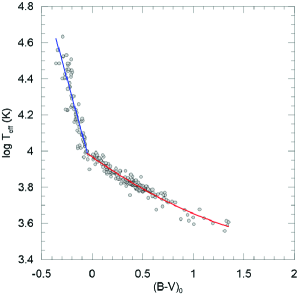
Figure 3: De-reddened colours ($(B-V)_{0}$) and published effective temperatures ($\log T_{eff}$) of stars in this study if the light ratio ($L_{2}/L_{1}$) is available both $B$ and $V$ bands (circles). The best fitting linear function (if $\log T_{eff}>4$) and the best fitting quadratic function (if $\log T_{eff}<4$) and the break point at $\log T_{eff}=4$ is clear.

3.4 $BC-T_{eff}$ relation

The $BC$ coefficients listed in Table 4 are shown together with the best fitting curve in Fig. 4. We have tried various degrees of polynomials to fit computed $BC$ data by the least squares method and found out that the best fitting function is a fourth degree polynomial with a standard deviation $\sigma=0.215$ and correlation coefficient $R^{2}=0.941$. The coefficients and associated uncertainties (Table 5) are determined by the least squares method and according to standard error analysis techniques of the least squares.

Figure 4: Computed $BC$ coefficients of 400 stars and best fitting curve (solid). Dotted lines are one sigma confidence limits (upper) and one-sigma deviations of data points from the $BC-T_{eff}$ curve (lower).

Table 6: Coefficients and associated uncertainties of the $BC-T_{eff}$ relation, which is a 4th degree polynomial, representing the main-sequence stars in the Solar neighbourhood.

$BC=a+b\times(\log T_{eff})+c\times(\log T_{eff})^{2}+d\times(\log T_{eff})^{3}+e\times(\log T_{eff})^{4}$
$a$	$b$	$c$	$d$	$e$
-2360.69565	2109.00655	-701.96628	103.30304	-5.68559
(519.80058)	(519.47090)	(194.29038)	(32.23187)	(2.00111)
$\sigma=0.215$,      $R^{2}=0.941$
valid in the range $3100<T_{eff}\leq 36000$ K
$BC=0.00$	$T_{eff,1}=5859$ K	$T_{eff,2}=8226$ K
$BC_{max}=0.095$	$T_{eff}=6897$ K
$BC_{\odot}=-0.016$	$T_{\odot}=5772$ K

According to Table 5, the $BC-T_{eff}$ relation found in this study has two roots, that is, it cuts $BC=0.00$ line twice at $T_{eff,1}=5859$ K, and $T_{eff,2}=8226$ K, thus the $BC$ values are positive ($BC>0$) between the temperatures $5859<T_{eff}<8226$ K. The maximum value $BC_{max}=0.095$, occurs at $T_{eff}=6897$ K. Bolometric correction for Solar-type stars with $T_{eff}=5772$ K is found to be $BC=-0.016$.

Readers should keep in mind that the $BC$ values computed according to the $BC-T_{eff}$ relation presented in Table 5 are for the main-sequence stars with Solar metallicity, $0.008\leq Z\leq 0.040$ corresponding to iron abundances $-0.28\leq\rm{[Fe/H]}\leq 0.61$ dex (Eker et al., 2018). Spectral type and $\log g$ distributions related to the $BC$ values will be discussed next.

3.5 Fundamental astrophysical parameters related to $BC$

A typical mass and a typical radius of a main-sequence star of a given effective temperature, within the Galactic disc at the Solar neighborhood with metallicities in the range $0.008\leq Z\leq 0.040$, were computed by using the interrelated MLR, MRR and MTR functions by Eker et al. (2018). Because the same sample of stars are used in this study to establish relations between effective temperatures related to un-reddened $B-V$ colours (Eqs. 12, 13) and BCs, we have completed Table 6 for interested readers who are looking for a single table listing spectral types, effective temperatures, intrinsic $B-V$ colours, bolometric corrections, absolute $V$ magnitudes, masses, radii and surface gravities.

Table 7: Fundamental astrophysical parameters related to $BC$ for nearby main-sequence stars with $0.008\leq Z\leq 0.040$.

SPT	$T_{eff}$	$(B-V)_{0}$	$BC$	$M_{V}$	$M$	$R$	$\log g$
	(K)	(mag)	(mag)	(mag)	($M_{\odot}$)	($R_{\odot}$)	(cgs)
O2	52483	-0.33*	-4.050	-6.913	63.980	16.734	3.797
O3	46990	-0.33*	-3.821	-5.996	44.260	12.312	3.904
O4	43251	-0.33*	-3.645	-5.424	34.809	10.301	3.954
O5	40738	-0.33*	-3.516	-5.057	29.669	9.236	3.980
O6	38282	-0.33*	-3.379	-4.708	25.380	8.362	3.998
O7	35810	-0.326	-3.229	-4.365	21.660	7.616	4.011
O8	33963	-0.314	-3.108	-4.113	19.215	7.131	4.016
O9	32211	-0.303	-2.984	-3.878	17.123	6.721	4.017
B0	29512	-0.284	-2.777	-3.520	14.277	6.171	4.012
B1	25119	-0.250	-2.382	-2.947	10.459	5.454	3.984
B2	21135	-0.213	-1.946	-2.430	7.699	4.967	3.933
B3	18408	-0.184	-1.595	-1.705	6.123	3.989	4.024
B5	15136	-0.142	-1.108	-0.872	4.516	3.214	4.079
B6	13964	-0.125	-0.918	-0.545	4.007	2.974	4.094
B7	13032	-0.110	-0.761	-0.268	3.625	2.797	4.104
B8	12023	-0.093	-0.588	0.053	3.234	2.617	4.113
B9	10666	-0.067	-0.356	0.535	2.743	2.394	4.119
A0	9886	-0.051	-0.228	0.848	2.478	2.274	4.119
A1	9419	-0.020	-0.156	0.904	2.325	2.362	4.058
A2	9078	0.021	-0.107	1.080	2.216	2.292	4.064
A3	8750	0.063	-0.062	1.259	2.113	2.226	4.068
A5	8222	0.136	0.000	1.569	1.952	2.123	4.075
A6	7980	0.171	0.025	1.723	1.879	2.077	4.078
A7	7745	0.207	0.045	1.879	1.810	2.033	4.080
A8	7534	0.241	0.060	2.026	1.749	1.994	4.082
F0	7161	0.305	0.077	2.302	1.643	1.928	4.084
F1	6966	0.340	0.081	2.457	1.588	1.893	4.085
F2	6792	0.373	0.080	2.602	1.540	1.863	4.085
F3	6637	0.403	0.077	2.735	1.498	1.838	4.085
F5	6397	0.453	0.064	3.225	1.354	1.588	4.168
F6	6310	0.472	0.058	3.404	1.305	1.508	4.197
F7	6223	0.491	0.050	3.581	1.259	1.434	4.225
F8	6152	0.507	0.042	3.727	1.222	1.377	4.248
G0	6026	0.536	0.026	3.986	1.161	1.283	4.286
G1	5957	0.552	0.016	4.129	1.128	1.236	4.307
G2	5888	0.569	0.005	4.270	1.098	1.191	4.327
G3	5848	0.579	-0.002	4.354	1.080	1.165	4.339
G5	5741	0.606	-0.022	4.585	1.031	1.097	4.371
G6	5689	0.619	-0.033	4.669	1.019	1.081	4.379
G7	5649	0.630	-0.042	4.732	1.011	1.069	4.385
G8	5559	0.654	-0.064	4.881	0.990	1.041	4.399
K0	5248	0.742	-0.158	5.421	0.922	0.951	4.447
K1	5070	0.797	-0.227	5.753	0.884	0.903	4.474
K2	4898	0.855	-0.306	6.092	0.848	0.858	4.500
K3	4732	0.914	-0.395	6.439	0.813	0.817	4.525
K5	4345	1.069	-0.661	7.327	0.736	0.727	4.582
M0	3802	1.353	-1.225	9.113	0.558	0.541	4.719
M1	3648	1.455	-1.438	9.643	0.524	0.508	4.745
M2	3499	1.569	-1.674	10.185	0.492	0.479	4.769
M3	3350	1.704	-1.943	10.773	0.462	0.452	4.793
M4	3148	1.946	-2.368	12.101	0.323	0.338	4.890
M5	2999	2.243	-2.736	13.055	0.249	0.284	4.928

(*) values taken from Sung et al. (2013).

Typical main-sequence masses for intermediate-mass and massive stars ($M>1.5M_{\odot}$) are computed from the effective temperatures given in column 2 using the mass-temperature relation (MTR). Once masses are known, then typical radii are computed from the luminosities estimated from the MLR function, according to Stefan-Boltzmann law. Since MTR and MLR functions are given for the stars with masses up to 31 $M_{\odot}$, $M$ and $R$ in the first three rows are extrapolated values. The surface gravity in the last column is then computed from the masses and radii listed in columns 6 and 7. Unfortunately, there is no single MTR function for the stars with the masses less than 1.5$M_{\odot}$. For those stars, MLR and MRR relations were used to estimate typical $M$ and $R$ for the main-sequence stars by checking up consistency between $L$, $R$ and $T_{eff}$ in the relation $L=4\pi R^{2}\sigma T_{eff}^{4}$, where $L$ and $R$ comes from MLR and MRR respectively, by trying different values of $M$.

Typical luminosities and corresponding absolute bolometric magnitudes are not listed in Table 6. Instead, absolute $V$ magnitudes, which are computed from absolute bolometric magnitudes according to Eq. (1), are given. The $BC$ values are calculated from the $BC-T_{eff}$ relation (Table 5) using $T_{eff}$ given in column 2. Despite the $BC-T_{eff}$ relation is valid for $3100<T_{eff}<36000$ K, the trend of the fitting curve (Fig. 4) encouraged us to extrapolate it for the first five rows and the last row rather than leaving those rows empty. That is, a single $BC-T_{eff}$ relation is used to calculate $BC$ of the main-sequence stars in the full range from the spectral type O2 to M5. While Eq. (12) is used to calculate intrinsic $B-V$ colours for early type hotter stars ($\log T_{eff}>4$) and Eq. (13) is used to calculate intrinsic $B-V$ colours for late type cooler stars ($\log T_{eff}<4$). The trend of intrinsic $B-V$ colours, however, did not encouraged us to extrapolate the linear relation (Eq. 12) to hotter stars, thus, $B-V$ colours of five rows in Table 6 are taken from Sung et al. (2013).

The columns of Table 6 are self consistent because all other columns are produced from column 2 by interrelated MLR, MRR, MTR (Eker et al., 2018) and the effective temperature, colour $(B-V)$ and bolometric correction relations found in this study. Correlation between the spectral types and the effective temperatures is not in the scope of this study. However, it is customary to include spectral types in the first columns of such tables. Therefore, we have used spectral types and effective temperatures of Sung et al. (2013).

4 Discussions

4.1 Comparisons to other determinations

The $BC-T_{eff}$ curve determined in this study is compared to other determinations in Fig. 5. It appears to have a reasonable agreement with Johnson (1966) and Sung et al. (2013) at low temperatures ($\log T_{eff}<3.86$), where the $BC$ values from Flower (1996) are smaller (more negative) from the lowest temperatures up to $\log T_{eff}\sim 3.6$ and the rest is about the same as the others up to $\log T_{eff}\sim 3.9$. The $BC$ values of this study appear to agree Flower (1996) and Sung et al. (2013) better than the $BC$ values of Johnson (1966), which appear relatively larger at high temperatures ($\log T_{eff}>3.86$). A noticeably good agreement between this study, Flower (1996) and Sung et al. (2013) at temperatures $\log T_{eff}\sim 3.96$ and $\log T_{eff}\sim 4.4$ deviates to be underestimated (more negative) away from these temperature points. $BC$ values of this study appears as if a straight line inclined towards lower (more negative) $BC$ values if $\log T_{eff}>3.96$. In this region, $BC$ values from Johnson (1966) are higher (less negative).

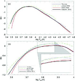
Figure 5: The $BC-T_{eff}$ relation is compared to other determinations (a) and at $T_{eff,max}\approx 6897$ K where it is enlarged to show details (b). Smoothness of the curve of this study is clear while the others with a sudden jump at $\log T_{eff}=3.7$ (Flower, 1996). Wavy appearance of Sung et al. (2013) curve is caused by limiting $BC$ into two digits (enlarging window).

In order to see more details in the comparison, Fig. 4b shows an enlarged region near at $T_{eff,max}\approx 6897$ K. The smoothness of the curve of this study is clear, while the others show sudden jumps. The jumps of the curve by Flower (1996) is clear at the connecting points of the polynomials assigned by him in the temperature ranges ($\log T_{eff}\geq 3.9$, $3.9<\log T_{eff}<3.7$, $\log T_{eff}\leq 3.7$). The wavy appearance of the curve by Sung et al. (2013) near the temperature maximum is caused by limiting the $BC$ values to two digits. To avoid such an effect, we preferred to adopt a $BC$ curve with $BC$ numbers which is in tree digits.

Fig. 6 shows the intrinsic $B-V$ colours of main sequence stars with metallicities $0.008\leq Z\leq 0.040$ in the Solar neighborhood which are compared to the intrinsic $B-V$ colours of the main-sequence stars according to Johnson (1966), Flower (1996) and Sung et al. (2013). A reasonable agreement of the four curves is clear.

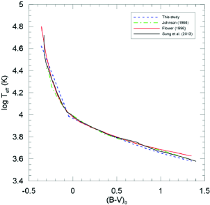
Figure 6: Intrinsic $B-V$ colours of main-sequence stars in this study is compared to colours of Johnson (1966), Flower (1996) and Sung et al. (2013).

4.2 Importance of reddening corrections

A reliable amount of reddening, in other words, an $E(B-V)$ colour excess of a star, is necessary for a reliable extinction. A reliable extinction is needed for a reliable absolute visual magnitude (Eq. 5). Being aware of the problem, all previous empirical $BC$ determinations (Johnson, 1964, 1966; Code et al., 1976; Flower, 1996) were done by assuming reddening is ignorable up to the distances 50-100 pc from the Sun (Leroy, 1993; Lallement et al., 2019) because of the local bubble. “Since most stars in these studies are bright and nearby, individual reddening values are generally very small and do not significantly contribute to the uncertainties in colours” said Flower (1996). Similarly, Code et al. (1976) stated that “$(B-V)_{0}$ is not an observed quantity for an individual star and uncertainties in interstellar extinction among our program stars contribute to the errors in determining a mean relation”, where $(B-V)_{0}$ is un-reddened colour of a star.

We think, this study is the first, which is not ignoring interstellar reddening up to several kpc, when computing empirical $BC$ coefficients in order to calibrate a $BC-T_{eff}$ relation. The most distant binary considered here is one of the brightest early type systems with O type components V467 Vel which has a distance of 6720 pc according to its trigonometric parallax $\varpi=0.1488\pm 0.096$ mas recorded in the Gaia DR2 (Gaia Collaboration et al., 2018). The biggest extinction $A_{V}$ used in this study belongs to an early type system MT91 372 with $A_{V}=7.01$ mag (Kiminki et al., 2015) which is a system having spectral types B1V+B5V at a distance of 1837 pc.

Importance of reddening corrections is visualized in Fig. 7 where the predicted $BC-T_{eff}$ curve of this study is plotted together with the $BC$ values if interstellar extinction is ignored in a linear scale. The components of MT91 372 and MT91 696, which are the systems with highest extinctions, are indicated. Most of the systems with late type components ($T_{eff}<5000$ K) are nearby systems thus their extinction could be ignorable. However, for other systems, especially, for the systems with components having $T_{eff}>5000$ K, necessity of the extinction correction is clear. Notice, that almost all stars are located below the $BC-T_{eff}$ curve if $T_{eff}>15000$ K.

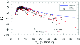
Figure 7: $BC-T_{eff}$ relation (solid) is plotted together computed $BC$ values (dots) if interstellar extinction is ignored.

Distribution of $V$ band extinctions is displayed in Fig. 8. The eight systems with extinctions bigger than 2 mag are not shown. The 68.9% of the whole sample have $V$ band extinctions smaller than 0.3 mag. Half of it, that is, 34% of the systems have extinctions smaller than 0.1 mag. It is clear on Fig. 7 that if we also chose nearby stars to avoid extinction, $BC-T_{eff}$ relation would have been depending upon about 70 systems (34% of the present sample) with components having effective temperatures less than 15000 K

Figure 8: The $V$ band extinction distribution of the present sample. The eight systems are not seen because their $A_{V}$ is bigger than 2 mag.

The extinctions ($A_{V}$) used in study are compared to the extinctions according to 3D reddening maps of Green et al. (2019) in Fig. 9. Concentration of data along the diagonal indicates a reasonable correlation despite several systems are scattered more than an expectation. For the sake of consistency, we preferred not to use the 3D reddening maps of Green et al. (2019) because of following reasons: 1) the method of computing $A_{V}$ is not applicable to all systems in this study. The 3D reddening maps of Green et al. (2019) are available for $\delta>-30^{o}$. 2) The reddening maps, whether they are 2D or 3D, all gives a mean reddening towards a direction. However, there could be systems with circum-binary dust redder than the mean value.

Figure 9: Comparison of extinctions of this study and the extinctions according to the 3D reddening maps of Green et al. (2019).

It is not a coincidence nor due to large random observational errors that the most scattered systems from the diagonal on Fig. 9 are from the private determinations, $Q$ method or SED. Our $A_{V}$ values estimated from the 2D maps of Schlafly & Finkbeiner (2011) seems to have better correlation than the five most scattered data from private determinations.

Figure 10: Distribution of 206 systems on the Galactic coordinates. The filled symbols show the systems with extinction estimated according to Galactic dust maps (Schlafly & Finkbeiner, 2011) and the empty circles are the systems which have extinction by private determinations (see references in Table 1).

Distribution of the present sample (206 systems) on the Galactic coordinates is given in Fig. 10, where the systems with extinction or $E(B-V)$ determined by various authors are shown by empty circles. The filled circles represents the systems $A_{V}$ calculated according to the method described NASA/IPAC Galactic Dust Reddening and Extinction maps of Schlafly & Finkbeiner (2011). Notice that almost all or most of the empty circles are located on the Galactic plane or near to it ($|b|<5^{o}$). There are some systems shown by filled circles with $|b|<5^{o}$ on Fig. 10, which must be nearby systems in the local bubble with small and ignorable extinction (Leroy, 1993; Lallement et al., 2019). It is also possible that extinction of a system is caused by circumstellar dust and it is more than the dust predicted from 2D extinction map of the Galaxy. So that, there could be systems located at high Galactic latitudes with unusual reddening, so we preferred to use private determinations $E(B-V)$ rather than Galactic dust maps.

5 Conclusions

Here, $BC-T_{eff}$ and $(B-V)_{0}-T_{eff}$ relations for main-sequence stars in the Solar neighborhood having metallicities in the range $0.008\leq Z\leq 0.040$ equivalent to an iron abundance distribution $-0.28\leq[{\rm Fe/H}]\leq 0.61$, are calibrated. The calibration sample is selected from detached eclipsing double-lined spectroscopic binaries because the most accurate mass, radii and temperatures could be obtained from their simultaneous LC and RV curves.

The $BC-T_{eff}$ and $(B-V)_{0}-T_{eff}$ relations were used together with interrelated MLR, MRR, and MTR relations from Eker et al. (2018) and a self consistent table of photometric ($B-V$, $BC$, $M_{V}$) and physical ($M$, $R$, $\log g$) parameters of nearby main-sequence stars are prepared (Table 6). It is a self consistent table because all the columns, except the first, are calculated analytically from typical $T_{eff}$ values of the main-sequence stars.

Accuracy of $BC-T_{eff}$ relation would be improved greatly in the future together with the improvements of trigonometric parallax measurements, in accord with expectation of Gaia DR3, and upgrading the detached eclipsing double-lined spectroscopic data by increasing the quality and the number.

6 Acknowledgments

Thanks to the anonymous referee whose comments were very useful. This work has been supported in part by the Scientific and Technological Research Council (TÜBİTAK) by the grant number 114R072. Thanks to Akdeniz University BAP office for providing a partial support for this research. This research has made use of NASA’s (National Aeronautics and Space Administration) Astrophysics Data System and the SIMBAD Astronomical Database, operated at CDS, Strasbourg, France and NASA/IPAC Infrared Science Archive, which is operated by the Jet Propulsion Laboratory, California Institute of Technology, under contract with the National Aeronautics and Space Administration. This work has made use of data from the European Space Agency (ESA) mission Gaia (https://www.cosmos.esa.int/gaia), processed by the Gaia Data Processing and Analysis Consortium (DPAC, https://www.cosmos.esa.int/web/gaia/dpac/consortium). Funding for the DPAC has been provided by national institutions, in particular the institutions participating in the Gaia Multilateral Agreement.

References

- Antonyuk & Rostopchina (2009) Antonyuk, K. A., Rostopchina, A. N., 2009, Ap, 52, 103
- Bahcall & Soneira (1980) Bahcall, J. N., Soneira, R. M., 1980, ApJS, 44, 73
- Bailer-Jones & Coryn (2015) Bailer-Jones, C. A. L., Coryn A. L., 2015, PASP, 127, 994
- Bailer-Jones et al. (2018) Bailer-Jones, C. A. L., Rybizki, J., Fouesneau, M., Mantelet, G., Andrae, R., 2018, AJ, 156, 58
- Bakış et al. (2007) Bakış, V. Bakış, H., Eker, Z., Demircan, O., 2007, MNRAS, 382, 609
- Bakış et al. (2018) Bakış, V., Yücel, G., Bakış, H., 2018, NewA, 65, 16
- Bayless & Orosz, (2006) Bayless, A. J., Orosz, J. A., 2006, ApJ, 651, 1155
- Bessell et al. (1998) Bessell, M. S., Castelli, F., Plez, B., 1998, A&A, 333, 231
- Bressan et al. (2012) Bressan, A., Marigo, P., Girardi, L., Salasnich, B., Dal Cero, C., Rubele, S., Nanni, A., 2012, MNRAS, 427, 127
- Budding et al. (2015) Budding, E., Butland, R., Blackford, M., 2015, MNRAS, 448, 3784
- Budding et al. (2017) Budding, E., Butland, R., Blackford, M., 2017, PASA, 30, 37
- Casagrande & VandenBerg (2018) Casagrande L., VandenBerg D. A., 2018, MNRAS, 475, 5023
- Cayrel et al. (1997) Cayrel, R., Castelli, F., Katz, D., van’t Veer, C., Gomez, A., Perrin, M.-N., 1997, Proceedings of the ESA Symposium ‘Hipparcos - Venice ’97’, 13-16 May, Venice, Italy, p. 433-436
- Chen et al. (2019) Chen, Y., Girardi, L., Fu, X., Bressan, et al., 2019, A&A, 632, A105
- Code et al. (1976) Code, A. D., Bless, R. C., Davis, J., Brown, R. H., 1976, ApJ, 203, 417
- Cousins (1981) Cousins, A. W. J., 1981, SAAOC, 6, 1
- Çiçek et al. (2017) Çiçek, C., Bulut, I, Bulut, A., 2017, AIP Conference Proceedings, Volume 1815, Issue 1, id.140003
- Eker et al. (2014) Eker, Z., Bilir, S., Soydugan, F., Yaz Gökçe, E., Soydugan, E., Tüysüz, M., Şenyüz, T., Demircan, O., 2014, PASA, 31, e024
- Eker et al. (2015) Eker, Z., Soydugan, F., Soydugan, E., et al., 2015, AJ, 149, 131
- Eker et al. (2018) Eker, Z., Bakış, V., Bilir, S., et al., 2018, MNRAS, 479, 5491
- Flower (1977) Flower, P. J., 1977, A&A, 54, 31
- Flower (1996) Flower, P. J., 1996, ApJ, 469, 355
- Gaia Collaboration et al. (2016) Gaia Collaboration, Prusti, T., de Bruijne, J. H. J., et al., 2016, A&A, 595, A1
- Gaia Collaboration et al. (2018) Gaia Collaboration, Brown, A. G. A., Vallenari, A., et al., 2018, A&A, 616, 22
- Girardi et al. (2008) Girardi, L., Dalcanton, J., Williams, B., et al., 2008, PASP, 120, 583
- Graczyk et al. (2019) Graczyk, D., Pietrzynski, G., Gieren, W., et al., 2019, ApJ, 872, 85
- Green et al. (2019) Green, G. M., Schlafly, E., Zucker, C., Speagle, J. S., Finkbeiner, D., 2019, ApJ, 887, 93
- Griffin & Griffin (2009) Griffin, R. E. M., Griffin, R. F., 2009, MNRAS, 394, 1393
- Haberreiter et al. (2008) Haberreiter, M., Schmutz, W., Kosovichev, A. G., 2008, ApJ, 675L, 53
- Hełminiak et al. (2009) Helminiak, K. G., Konacki, M., Ratajczak, M., Muterspaugh, M. W., 2009, MNRAS, 400, 969
- Hełminiak & Konacki (2011) Helminiak, K. G., Konacki, M., 2011, A&A, 526A, 29
- Heintze (1973) Heintze, J. R. W., 1973, Proceedings of IAU Symposium no. 54 Held in Geneva, Switzerland, Sept. 12-15, 1972. Ed by B. Hauck and Bengt E. Westerlund. Dordrecht, Boston, Reidel, p.231
- Irwin et al. (2006) Irwin, J., Charbonneau, D., Berta, Z. K., et al., 2009, ApJ, 701, 1436
- Jeffries et al. (2013) Jeffries, M. W., J., Sandquist, E. L., Mathieu, R. D., et al., 2013, AJ, 146, 58
- Johnson & Morgan (1953) Johnson, H. L., Morgan, W. W., 1953, MNRAS, 113, 468
- Johnson (1964) Johnson, H. L., 1964, Boletin de los Observatorios de Tonantzintla y Tacubaya, 3, 305
- Johnson (1966) Johnson, H. L., 1966, ARA&A, 4, 193
- Kiminki et al. (2015) Kiminki, D. C., Kobulnicky, H. A., Vargas Alvarez, C. A., Alexander, M. J., Lundquist, M. J., 2015, ApJ, 811, 85
- Kjurkchieva & Marchev (2007) Kjurkchieva, D. P., Marchev, D. V., 2007, MNRAS, 381, 663
- Kuiper (1938) Kuiper, G. P., 1938, ApJ, 88, 472
- Lallement et al. (2019) Lallement, R.,Babusiaux, C., Vergely, J. L., Katz, D., Arenou, F., Valette, B., Hottier, C., Capitanio, L., 2019, A&A, 625A, 135
- Lazaro et al. (2015) Lazaro, C., Arevalo, M. J., Almenara, J. M., 2015, NewA, 34, 139
- Leroy (1993) Leroy, J. L., 1993, A&A, 274, 203
- Malagnini et al. (1985) Malagnini, M. L., Morossi, C., Rossi, L., Kurucz, R. L., 1985, A&A, 152, 117
- Marshall et al. (2006) Marshall, D. J., Robin, A. C., Reylé, C., Schultheis, M., Picaud, S., 2006, A&A, 453, 635
- McDonald & Underhill (1952) McDonald, J., K., Underhill, A., B., 1952, ApJ, 115, 577
- North et al. (1997) North, P., Studer, M., Kunzli, M., 1997, A&A, 324, 137
- Pettit & Nicholson (1928) Pettit, E., Nicholson, S. B., 1928, ApJ, 68, 279
- Popper (1959) Popper, D., M., 1959, ApJ, 129, 647
- Popper (1986) Popper, D. M., Lacy, C. H., Frueh, M. L., Turner, A. E., 1986, ApJ, 91, 383
- Rozyczka et al. (2009) Rozyczka, M., Kaluzny, J, Pietrukowics, P., Pych, W., Mazur, B., Catelan, M., Thompson, B. T., 2009, AcA, 59, 385
- Sandquist et al. (2013) Sandquist, E. L., Shetrone, M., Serio, A. W., Orosz, J., 2013, AJ, 146, 40
- Schlafly & Finkbeiner (2011) Schlafly, E. F., Finkbeiner, D. P., 2011, ApJ, 737, 103
- Shkolnik et al. (2008) Shkolnik, E., Liu, M. C., Reid, I. N., Hebb, L., Cameron, A. C., Torres, C. A., Wilson, D. M., 2008, ApJ, 682, 1248
- Siviero et al. (2004) Siviero, A., Munari, U., Sordo, R., Marrese, P. M., 2004, ASPC, 318, 182
- Soydugan et al. (2013) Soydugan, F., Soydugan, E., Kanvermez, Ç., Liakos, A., 2013, MNRAS, 432, 3278
- Standish (1995) Standish, E. M., 1995, Highlights of Astronomy, 10, 180
- Sung et al. (2013) Sung, H., Lim, B., Bessell, M. S., Kim, J. S., Hur, H., Chun, M., Park, B., 2013, JKAS, 46, 103
- Tomasella et al. (2008) Tomasella, L., Munari, U., Siviero, A., Cassisi, S., Dallaporta, S., Zwitter, T., Sordo, R., 2008, A&A, 480, 465
- Torres (2010) Torres, G., 2010, AJ, 140, 1158
- van Hamme & Wilson (2007) van Hamme, W., Wilson, R. E., 2007, ApJ, 661, 1129
- van Leeuwen (2007) van Leeuwen, F., 2007, A&A, 474, 653
- Volkov & Chochol (2007) Volkov, I. M., Chochol, D., 2014, CoSka, 43, 419
- Wildey (1963) Wildey, R. L., 1963, Nature, 199, 988
- Wilson & van Hamme (2014) Wilson, R. E., van Hamme, W., 2014, ApJ, 780, 151
- Young et al. (2006) Young, T. B., Hidas, M. G., Webb, J. K., Ashley, M. C. B., Christiansen, J. L., Derekas, A., Nutto, C., 2006, MNRAS, 370, 1529
- Zola et al. (2014) Zola, S., Şenavcı, H. V., Liakos, A., Nelson, R. H., Zakrzewski, B., 2014, MNRAS, 437, 3718