Comparing Moment-Based and Monte Carlo Methods of Radiation Transport Modeling
for Type II-Plateau Supernova Light Curves

Abstract

Time-dependent electromagnetic signatures from core-collapse supernovae are the result of detailed transport of the shock-deposited and radioactively-powered radiation through the stellar ejecta. Due to the complexity of the underlying radiative processes, considerable approximations are made to simplify key aspects of the radiation transport problem. We present a systematic comparison of the moment-based radiation hydrodynamical code STELLA and the Monte Carlo radiation transport code Sedona in the 1D modeling of Type II-Plateau supernovae. Based on explosion models generated from the Modules for Experiments in Stellar Astrophysics (MESA) instrument, we find remarkable agreements in the modeled light curves and the ejecta structure thermal evolution, affirming the fidelity of both radiation transport modeling approaches. The radiative moments computed directly by the Monte Carlo scheme in Sedona also verify the accuracy of the moment-based scheme. We find that the coarse resolutions of the opacity tables and the numerical approximations in STELLA have insignificant impact on the resulting bolometric light curves, making it an efficient tool for the specific task of optical light curve modeling.

1 Introduction

Most massive stars with stellar mass above 8 $M_{\odot}$ end their lives in energetic core-collapse supernova (CCSN) explosions, whose electromagnetic signatures contain information about the progenitor stars and their final moments. The most common subclass of CCSNe are of Type II-Plateau (II-P) (Li et al., 2011; Smith et al., 2011), explosions of red supergiants (RSG) (Woosley et al., 2002; Heger et al., 2003; Smartt et al., 2009; Smartt, 2015; Van Dyk et al., 2012a, b) with prolonged release of shock energy powering the characteristic plateaus in their light curves.

Current time-domain survey facilities, e.g., the Zwicky Transient Facility (ZTF, Bellm et al., 2019) and the All-Sky Automated Survey for Supernovae (ASAS-SN, Kochanek et al., 2017), as well as the deployment of the Vera C. Rubin Observatory (LSST Science Collaboration et al., 2009), will significantly increase our capacity to explore SN populations. An important goal in these studies will be to reconcile the variety of observed SN events with the properties of their massive star progenitors and resulting explosions.

In light of the imminent expansion of photometric data, the inverse problem of inferring progenitor and explosion properties from observed light curves represents a key challenge in achieving physical understanding of the full II-P SNe population. Developments in 3D simulations have advanced our understanding of RSG explodability and observational CCSN signatures (Wongwathanarat et al., 2015; Janka et al., 2016; Vartanyan et al., 2019; Burrows et al., 2020), but the enormous demands in computing resources limit the exploration of large suites of multi-dimensional progenitor and explosion models. Synthetic light curves, on the other hand, can be generated relatively quickly with one-dimensional (1D) radiation hydrodynamical or radiation transport models based on 1D progenitor and explosion models.

A valuable approach to deriving light curves from RSG progenitors is via a combination of radiation hydrodynamical and radiation transport simulations. In the radiation hydrodynamics step, stellar progenitors of II-P SNe are constructed with a stellar evolution code, and explosions are simulated by either a moving piston or a thermal bomb near the inner boundary (Woosley & Weaver, 1995; Woosley & Heger, 2007; Dessart & Hillier, 2010, 2011). The resulting ejecta structures are the initial conditions for the radiation transport modeling of photometric and spectral features. Kasen & Woosley (2009) adopted this approach to compute the broadband light curves and spectral evolution with the multi-wavelength Monte Carlo radiation transport code Sedona. This approach allowed close examination of the dependence of light curve diagnostics on the progenitor model parameters and the refinement of analytical scaling formulae (Popov, 1993).

Similar approaches have been applied to build the observable-progenitor parameter relation (see, e.g. Dessart et al., 2013; Morozova et al., 2016; Sukhbold et al., 2016). More recently, suites of progenitor and explosion models have highlighted the high degree of degeneracy between light curve features/photospheric velocities and model parameters (Dessart & Hillier, 2019; Goldberg et al., 2019; Martinez & Bersten, 2019). While photometric and spectral observables are useful in constraining the model parameters, they do not offer associations to unique sets of progenitor properties after $\approx 20$ days. Before this time, when the ejecta is still accelerating and the emission comes from the outer $<0.1M_{\odot}$ of material, photospheric velocities might distinguish between otherwise degenerate light curves. However, such measurements are rare and prone to modifications by the uncertain circumstellar environment (e.g. Moriya et al. 2018).

Observable signatures from II-P SNe are the results of the complex interplay between radiation and the structures, compositions, and opacities of the ejecta. The predicted observable characteristics may also be sensitive to the numerical schemes used for radiation transport. For example, Martinez & Bersten (2019) and Dessart & Hillier (2019) both adopted the gray diffusion approximation during the hydrodynamical evolution step, light curves and spectra in Dessart & Hillier (2019) were produced using a more sophisticated, wavelength-dependent non-local thermodynamical equilibrium (non-LTE) scheme. Discrepancies may also be introduced for other practical reasons, such as the use of an opacity floor (Morozova et al., 2015; Martinez & Bersten, 2019).

The effects of the choice of radiation transport schemes have been evaluated in the context of radiation-driven gas dynamics (Krumholz & Thompson, 2012; Davis et al., 2014; Rosdahl & Teyssier, 2015; Tsang & Milosavljević, 2015; Zhang & Davis, 2017). In transient signature predictions, several works have attempted to verify the accuracy of different numerical radiation transport approaches. Kozyreva et al. (2017) have compared pair-instability SN light curves produced by different codes. However, verification works for II-P SNe are very scarce, and they are usually based on a handful of progenitor models and on visual inspections only (Morozova et al., 2015; Kozyreva et al., 2019).

In this paper, we focus on the II-P SNe and conduct a detailed comparison between the moment-based radiation hydrodynamics code STELLA and the particle-based Monte Carlo radiation transport code Sedona. We make direct comparisons of the light curves and ejecta profiles. We note that the numerical approximations and ray-tracing radiation transport scheme in STELLA offer significant speedup over Sedona’s detailed opacity calculations and Monte Carlo sampling. Our goals are to assess and quantify the differences yielded by the two fundamentally different radiation transport approaches, to understand the impacts different radiation treatments entail, and to offer confidence in the interpretations of similar light curve analyses.

In Section 2, we discuss the numerical methodology with emphasis on the aspects related to radiation transport, and describe our progenitor and explosion model suite. In Section 3, we present the results of the numerical experiment and compare the two radiation transport methods. In Section 4, we summarize our findings and discuss potential future directions.

2 Numerical Methods

We use three numerical tools to model the hydrodynamics of the massive star progenitor and the radiation transport in the expanding ejecta. The progenitor evolution and traversal of the shock within the star are calculated using MESA (Paxton et al., 2011, 2013, 2015, 2018, 2019). The emergent light curves and the ejecta properties are calculated with the moment-based, radiation hydrodynamics code STELLA (Blinnikov et al., 1998; Blinnikov & Sorokina, 2004; Baklanov et al., 2005; Blinnikov et al., 2006) and the particle-based, Monte Carlo radiation transport code Sedona (Kasen et al., 2006).

2.1 Modeling Red Supergiants and their Explosions in MESA

The progenitor stellar models were selected from Paxton et al. (2018), the standard suite of models in Goldberg et al. (2019), and models motivated by matching observations described in Goldberg & Bildsten (2020).

The inlist parameter files for these progenitor models follow those used in Paxton et al. (2018), namely, from the test_suite case example_make_pre_ccsn with revised values for the progenitor mass, mixing length in the H-rich envelope, initial rotation, core overshooting, and the initial metallicity set to solar ($Z~{}=~{}0.02$)

After removing the core, a thermal bomb is injected into the innermost 0.01$M_{\odot}$ of each model, which heats the star to a specified total final energy $E_{\rm exp}$. The evolution of the shock is then modeled in MESA with the “Duffell RTI” prescription for mixing from Rayleigh-Taylor Instability (Duffell, 2016; Paxton et al., 2018), with the modeling terminating at shock breakout. All models remove fallback onto the inner boundary as described in Paxton et al. (2019) and Goldberg et al. (2019). We focus on models at sufficiently high explosion energy that fallback is negligible. Radioactive ⁵⁶Ni distributions are scaled to match the total nickel mass desired.

The MESA models at the moment of shock breakout are handed off to STELLA as described in Paxton et al. (2018). Our models have no additional material outside the stellar photosphere. The spatial zoning in the STELLA input files is determined by interpolating across the MESA profiles to match a specified number of zones. The models are then evolved from near-shock breakout to day 170 (see Paxton et al. (2018) for more details). We used 400 spatial zones and $N_{\textrm{freq}}=40$ frequency bins in STELLA, as convergence studies (Paxton et al., 2018) showed sufficient agreement in bolometric light curves at this choice of resolution.

Table 1: Summary of the RSG progenitor and explosion models with the corresponding ejecta properties. The models are named after the concatenation of the ejecta mass, progenitor radius at shock breakout, explosion energy, and the nickel mass (if any). The notation follows M$[M_{\textrm{ej}}]$_R[$R$]_E[$E_{\textrm{Exp}}$](_Ni[$M_{\textrm{N}i}$]).

Model Name	$M_{\textrm{ZAMS}}$	$M_{\textrm{final}}$	$M_{\textrm{c,He}}$	$M_{\textrm{H,tot}}$	$X_{\textrm{He,env}}$	$t_{\textrm{SB}}$
($M_{\odot}$)($R_{\odot}$)(1051 erg)(10-2 $M_{\odot}$)	($M_{\odot}$)	($M_{\odot}$)	($M_{\odot}$)	($M_{\odot}$)		(day)
Nickel-Rich Suite
M9.3_R433_E0.5_Ni1.5	11.8	10.71	3.58	4.65	0.33	1.10
M9.3_R433_E1.0_Ni3.0						0.70
M9.3_R433_E2.0_Ni6.0						0.40
‡M12.7_R719_E0.84_Ni4.8	15.0	14.53	5.09	6.37	0.31	1.63
†*M16.3_R608_E1.0_Ni4.5	19.0	17.79	5.72	7.53	0.34	1.37
†*M16.3_R608_E2.0_Ni3.0						0.97
†*M16.3_R608_E2.0_Ni7.5						0.97
Nickel-Poor Suite
M9.3_R433_E0.5	11.8	10.71	3.58	4.65	0.33	1.10
M9.3_R433_E0.8						0.78
M9.3_R433_E1.0						0.70
M9.3_R433_E2.0						0.50
†*M16.3_R608_E1.0	19.0	17.79	5.72	7.53	0.34	1.37
†*M16.3_R608_E2.0						0.97
Exploratory Suite
‡M7.9_R375_E0.23_Ni4.3	10.0	9.41	3.15	4.06	0.33	1.13
‡M16.5_R533_E4.6_Ni13.0	19.0	18.09	6.28	8.04	0.31	0.55
†Stripped_M4.7_R379_E1.0_Ni3.0	17.0	6.39	6.25	0.10	0.67	0.28

2.2 Model Selection

We compiled a characteristic set of models to capture the variations of CCSN progenitor properties. Models are divided into three suites. The nickel-rich suite consists of models typical of II-P SNe. The nickel-poor models have no radioactive nickel. The goal is to compare the radiation transport results in the absence of radioactive power. We also explore models unlike common II-P SNe in the exploratory suite. In particular, we test models with extreme values of $M_{\rm Ni}$ and $E_{\rm exp}$. The M7.9_R375_E0.23_Ni4.3 model is motivated by SN2009ib, which had an unusually long plateau (Takáts et al., 2015); the M16.5_R533_E4.6_Ni13 model is informed by the energetic II-P event SN2017gmr (Andrews et al., 2019). The Stripped_M4.7_E1.0_Ni03 model is not a typical II-P SN – it is a model with most of its hydrogen stripped to resemble a II-b SN. We include this model to test the reliability of radiation transport modeling when gamma-rays are not fully trapped.

The model names and their key properties of the progenitor and explosion are summarized in Table 1. The time to shock breakout $t_{\textrm{SB}}$ is included to indicate the relative expansion times, and the helium fraction in the envelope $X_{\textrm{He,env}}$ is provided for reference as helium abundance can modify the plateau duration and brightness (Kasen & Woosley, 2009).

2.3 Evolution to Homology and Handoff to Sedona

Sedona does not follow ejecta hydrodynamics. Therefore, models from STELLA must be handed off as inputs to Sedona, at a time late enough so that further hydrodynamical evolution is insignificant, and early enough to capture meaningful radiation signatures.

In the course of the evolution with STELLA, the outer $\approx$75% of the ejecta mass establishes homology by about 5 days after shock breakout. In the outer region, assuming homology thereafter introduces $\leq$5% difference in the velocity field from the hydrodynamical calculation. Beyond $\approx$5 days, the largest deviations from homology appear only near the inner boundary of the ejecta, where the reverse shock is sometimes still moving inward.

By default, Sedona evolves the ejecta assuming homology, i.e. radius of the $i$th spatial zone evolves as $r_{i}(t_{\rm exp})=v_{i}\,t_{\rm exp}$, where $v_{i}$ is the time-independent zone velocity and $t_{\rm exp}$ is the time since explosion. However, the conventional $r=v\,t$ homology assumption does not strictly apply for Type II-P SNe due to the large progenitor radii. We modified Sedona to incorporate this difference – by setting $r_{i}(t^{\prime})=r_{i,{\rm handoff}}+v_{i}\,t^{\prime}$, taking into account its initial radius at model handoff, and $t^{\prime}$ is the time since handoff. Sedona then evolves the ejecta density structure assuming that the mass contained in each zone remains constant, and the zone volume is updated by our revised radius relation.

We need to ensure that the velocity profiles of the ejecta models are sufficiently time-invariant. The actual time after the STELLA-to-Sedona handoff when homology in the entire ejecta is established depends on the specific models. We choose day 20 after shock breakout as the STELLA-to-Sedona handoff time, as by then most of the ejecta energy is in kinetic rather than internal energy. This choice is consistent with the timescale for establishing homology found in Utrobin et al. (2017) for II-Ps with a different 1D code CRAB. In all our models, the time to shock breakout $t_{\textrm{SB}}~{}<~{}2$ days. Taking $t_{\textrm{SB}}$ to be the characteristic timescale for the SN expansion, model handoff at day 20 corresponds to $>10$ expansion times after the explosion.

At the day-20 handoff, radial profiles from STELLA, which contain the zone radius, radial velocity, gas density and temperature, and the abundances of 15 atomic species, are copied onto a 1D spherically symmetric, Lagrangian grid in Sedona without regridding. In other words, Sedona sees an identical ejecta on the same grid as STELLA at the moment of handoff. Once handed off, Sedona performs Monte Carlo radiation transport and ejecta evolution fully independent of STELLA up to day 200 (150) for nickel-rich/exploratory (nickel-poor) models.

2.4 Radiation Transport in STELLA and Sedona

STELLA solves the time- and frequency-dependent moment equations of radiation intensity on a Lagrangian 1D spherical grid. The system of two moment equations are closed by a variable Eddington factor, which is computed by integrating the time-independent transport equation for each frequency bin using a ray tracing integration scheme (Zhang & Sutherland, 1994; Blinnikov et al., 1998).

A low number of logarithmically-spaced frequency bins $N_{\rm freq}=40$ is used to span the wavelength range $1-50,000$ Å. The radiation source terms are coupled to the equations of hydrodynamics and solved implicitly (Blinnikov et al., 1998). For thermal radiation, the following sources of opacity are taken into account: bound-free/photoionization (Verner et al., 1993), free-free (Gronenschild & Mewe, 1978), bound-bound/line opacity (Kurucz & Bell, 1995; Verner et al., 1996), and electron scattering. Bound-bound opacity is included using the Sobolev approximation under the line expansion formalism (Karp et al., 1977; Eastman & Pinto, 1993). The Sobolev line optical depth of the $i$th bound-bound transition is given by

$$\tau_{\rm sob,i} =\frac{\pi e^{2}}{m_{\textrm{e}}c}f_{i}n_{i}\lambda_{i}\cdot t_{\rm exp},$$ (1)

where $f_{i}$ is the oscillator strength of the transition, $n_{i}$ is the number density of the lower atomic level of the transition, $\lambda_{i}$ is the line center rest wavelength, and the $t_{\rm exp}$ term follows from the velocity gradient of the homologously expanding SN ejecta. In our models, $t_{\textrm{exp}}$ is taken to be the time since shock breakout, i.e., MESA-to-STELLA handoff. In this formalism, the large velocity gradient Doppler shifts photons into resonance with each lines in a frequency bin exactly once, and the lines are treated as non-overlapping. Line opacity is further assumed to be fully absorptive, an approximation justified by non-LTE calculations (Baron et al., 1996; Pinto & Eastman, 2000).

For gamma-rays, STELLA uses the one-group approximation, which effectively treats the transport and deposition of gamma-ray energy with a gray absorption opacity (Swartz et al., 1995). Furthermore, kinetic energy of the positrons resulting from ⁵⁶Co decays is assumed to be deposited locally (Blinnikov et al., 2006). The bolometric light curves are computed by summing the radiative fluxes over all frequency bins.

In the public version of STELLA, opacity tables are constructed on a fixed grid of density and temperature, with $\log(\rho/\rm{g\,cm}^{-3})$ spanning from -18 to -4, and $\log(T/\rm{K})$ from 3.4 to 6.2, each with $N_{\rm grid}~{}=~{}14$ grid points uniformly separated in the logarithmic space. To keep the calculations tractable, opacity tables are only computed at six times at $(t/\rm{days})\in\{1,2.5,6.3,15.8,39.8,100\}$ after shock breakout, and on a reduced number of $N_{\rm reduced}=50$ uniformly spaced spatial zones. In the more recent, private version of STELLA (Blinnikov et al., 2006), the last two approximations have been removed and the opacity is computed at every time step for every zone, but these new features are not yet publicly available. Ionization fractions and level populations of the 15 tracked atomic species are followed using the LTE approximation. A simplification is made to include only the six most populated ionization stages. The pre-computed opacity tables are interpolated in the course of STELLA’s radiation hydrodynamical evolution.

The default $\log(T/\textrm{K})$ resolution of the opacity tables is too coarse across the hydrogen recombination temperature ($\log(T_{\rm recomb}/\rm{K})\approx 3.7$) and it reduces the accuracy of radiation transport in II-P ejecta as the opacity varies sharply across the recombination front. We thus modified the public version to allow a finer opacity grid with $N_{\rm grid}=56$ and $N_{\rm reduced}=200$. In addition, we appended the stimulated emission correction term, $1-\exp{(hc/\lambda_{i}k_{\rm B}T)}$, to the Sobolev optical depth of the line expansion opacity, Equation (1). These improvements lead to smoother ejecta structures and bolometric light curves, and they will be available in an upcoming MESA release. In the following, modeling results from our modified version of STELLA are presented unless otherwise specified.

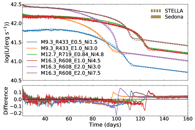
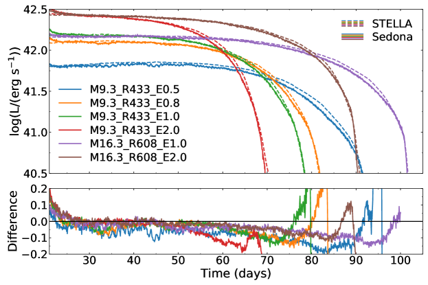
Figure 1: Bolometric light curves from Sedona (solid) and STELLA (dashed) for the nickel-rich (top) and nickel-poor (bottom) suites. Relative differences between the bolometric luminosities computed by Sedona and STELLA, defined as $(L_{\texttt{Sedona}}-L_{\texttt{STELLA}})/L_{\texttt{Sedona}}$, are shown in the lower panels.

Time-dependent, multi-frequency radiation transport is also performed with the Monte Carlo code Sedona (Kasen et al., 2006). Monte Carlo methods directly solve the radiation transfer equation by discretizing the radiation field into individual photon packets. Sampling the emission, absorption, and scattering of the packets through space and time yields a statistical approximation to the solution of the transfer equation. Monte Carlo methods are fundamentally different from moment-based methods. We adopt the mixed-frame formalism for the Monte Carlo radiation transport (Mihalas & Klein, 1982) – emissivity and opacity are defined in the fluid co-moving frame, while the quantities are Lorentz-transformed into the lab frame where radiation transport is carried out. Unlike STELLA, Sedona is optimized to handle much denser frequency grids. However, to facilitate direct comparison, we used frequency limits and resolution that match STELLA’s default.

The temperature structure is evolved in Sedona by considering the expansion, the radioactive heating from the decay of ⁵⁶Ni and ⁵⁶Co, and radiative transport in each zone. The ionization structures and level populations are determined assuming LTE. For thermal radiation, the same types of opacity are included, namely, bound-free, free-free, bound-bound, and electron scattering. We note that the bound-free and free-free opacities are computed from a different set of analytical formulae than that used by STELLA. Following the common practice, we assume line opacity to be purely absorptive. A large number of $N_{\textrm{init}}=10^{7}$ Monte Carlo photon packets are used to represent the initial thermal radiation field at model handoff. An additional $N_{\textrm{nuc}}=10^{5}$ packets are added per radiation transport time step to sample the radioactive luminosity in those models containing ⁵⁶Ni.

The Monte Carlo radiation treatment allows Sedona to self-consistently handle the frequency-dependent transport and thermalization of gamma-rays (Kasen et al., 2006). Positrons produced during the nuclear decays are assumed to be thermalized instantaneously into photons, but their energies can be deposited non-locally depending on the opacity along the photons’ trajectories.

To properly set the time step size for the homology evolution in Sedona, we consider the relevant timescales of radiation transport. In the lab frame where Sedona’s radiation transport is performed, the radiative flux comprises both the diffusion and advection contributions. In spherical symmetry, the transformation to $\mathcal{O}(v/c)$ is (Mihalas & Weibel-Mihalas, 1999),

$$F_{\rm r} =F_{\rm r,0}+v(r)\cdot(E_{\rm r,0}+P_{\rm r,0}),$$ (2)

$$=F_{\rm diff,0}+F_{\rm adv,0},$$ (3)

where $E_{\rm r,0}$, $F_{\rm r,0}$, and $P_{\rm r,0}$ denote the radiation energy density, flux, and pressure measured in the co-moving fluid frame, $v(r)$ is the radial velocity, and $F_{\rm r}$ without the subscript ‘$0$’ denote the lab frame radiative flux. The two terms on the right hand side of Equation (2) can be respectively identified as the diffusive and advective flux. The characteristic timescales for radiative diffusion and advection across the local shell thickness of the spherical grid, $\Delta r$, are

$$t_{\rm diff} =E_{\rm r,0}\Delta r/F_{\rm diff,0},$$ (4)

$$t_{\rm adv} =E_{\rm r,0}\Delta r/F_{\rm adv,0}.$$ (5)

In the optically thick regime, these expressions simplify by invoking the Fick’s law of radiation transfer and assuming isotropy ($P_{\rm r,0}=E_{\rm r,0}/3$),

$$t_{\rm diff} \approx E_{\rm r,0}\Delta r\left[\frac{c}{3}\frac{dE_{\rm r,0}}{d\tau}\right]^{-1}\approx\frac{3}{c}\tau(r)\Delta r,$$ (6)

$$t_{\rm adv} \approx\frac{3}{4}\frac{\Delta r}{v(r)},$$ (7)

where $\tau(r)$ is the optical depth to infinity from radius $r$. By equating $t_{\textrm{diff}}$ and $t_{\textrm{adv}}$ in Equation (6) and (7), we obtain a characteristic optical depth $\tau_{\textrm{char}}=c/4v$ below which radiation is no longer locally trapped by diffusion and radiation transport is expected to modify the ejecta’s thermal structures.

In SNe, the dynamics of the ejecta are dominated by the expansion. For the Sedona models, we therefore chose a constant time step size of 0.05 day, which is $\lesssim$0.1 $t_{\rm adv}$ throughout the entire duration of the simulations. Light curves are generated by tallying the Monte Carlo photon packets that escape the ejecta through the outer boundary.

Table 2: Comparison of light curve diagnostics from the STELLA and Sedona modeling. The plateau duration $t_{\textrm{p}}$ is computed using the same procedure as in Goldberg et al. (2019).

	$L_{\rm 50}$/1042 erg s-1			$t_{\rm p}$/days
Model	STELLA	Sedona	% Difference	STELLA	Sedona	% Difference
Nickel-Rich Suite
M9.3_R433_E0.5_Ni1.5	0.70	0.67	-4.3	104.2	106.7	2.3
M9.3_R433_E1.0_Ni3.0	1.371	1.374	0.2	89.16	87.75	-1.6
M9.3_R433_E2.0_Ni6.0	2.17	2.25	3.9	81.9	80.2	-2.1
M12.7_R719_E0.84_Ni4.8	1.54	1.53	-0.3	116.6	119.5	2.4
M16.3_R608_E1.0_Ni4.5	1.46	1.49	2.2	120.8	119.8	-0.8
M16.3_R608_E2.0_Ni3.0	2.43	2.39	-1.7	97.4	96.6	-0.8
M16.3_R608_E2.0_Ni7.5	2.45	2.45	$<10^{-3}$	108.5	107.9	-0.5
Nickel-Poor Suite
M9.3_R433_E0.5	0.70	0.66	-6.2	93.8	95.7	2.0
M9.3_R433_E0.8	1.18	1.15	-2.1	84.0	83.8	-0.2
M9.3_R433_E1.0	1.37	1.34	-2.1	83.6	80.0	-3.1
M9.3_R433_E2.0	1.99	1.93	-3.4	70.2	70.5	0.5
M16.3_R608_E1.0	1.48	1.39	-5.9	105.0	102.6	-2.3
M16.3_R608_E2.0	2.45	2.42	-1.3	90.0	91.5	1.7

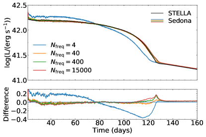
Figure 2: Bolometric light curves of the M12.7_R719_E0.84_Ni4.8 model using different numbers of frequency bins. The wavelength range for radiation transport is held fixed at 1$-$50000 Å for this numerical experiment. In both codes, the frequency grids are uniform in $\log$(frequency) space. The light curves converge once $N_{\textrm{freq}}\geq 40$, the default value in STELLA. Relative differences between the light curves from Sedona and STELLA, defined as $(L_{\texttt{Sedona}}-L_{\texttt{STELLA}})/L_{\texttt{Sedona}}$, are shown in the bottom panel.

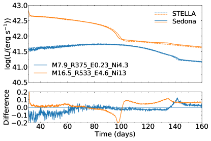
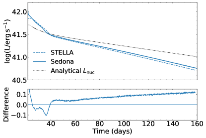
Figure 3: Bolometric light curves from the exploratory suite. The II-P models M7.9_R375_E0.23_Ni4.3 and M16.5_R533_E4.6_Ni13 with extreme $M_{\textrm{ej}}/E_{\textrm{Exp}}$ are shown in the left panel. The II-b-like model Stripped_M4.7_E1.0_Ni03 model is shown on the right. The black dotted line on the right panel shows the total nuclear decay energy production rate integrated over the entire ejecta. The relative differences between the Sedona and STELLA light curves, defined as $(L_{\texttt{Sedona}}-L_{\texttt{STELLA}})/L_{\texttt{Sedona}}$, are shown in the bottom panels.

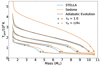
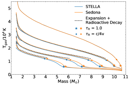
Figure 4: Gas temperature evolution of the M9.3_R433_E1.0(_Ni3.0) model is displayed on the left (right) panel. The lines correspond to, from top to bottom, profiles at day 20, 30, 40, 50, and 60. The stars mark the locations of the photosphere. The circular points denote where $\tau_{\textrm{R}}=c/4v$. The black dashed lines are the analytical scaling relations – on the left panel we use adiabatic evolution, $T_{\rm gas}(t)=T_{\rm gas}({\rm day\,20})(t/20\,{\rm days})^{-1}$; on the right the total local deposition of radioactive decay energy is assumed (Nadyozhin, 1994, Equation (13))). Both analytical relations are truncated at $\tau_{\textrm{R}}=c/4v$.

3 Results

3.1 Bolometric Light Curves

The top panels of Figure 1 compare the light curves from the representative models in the nickel-rich and nickel-poor suites, as computed by Sedona (solid) and STELLA (dashed). The lower panels below the light curves show the relative difference between the two. The moment-based radiation transport scheme of STELLA matches well the Monte Carlo approach of Sedona following handoff at day 20. During the plateau phase, the bolometric luminosities between the two methods agree within 5%. The systematic bias of STELLA models towards higher luminosity during the plateau is from its hydrodynamical evolution. Following handoff, a small fraction of internal energy is still being converted into kinetic energy. At day 100, the residual acceleration results in a $\approx$3% increase in radius in the majority of the ejecta compared to a constant-velocity evolution, giving rise to a $\approx$10% reduction in density as compared to Sedona (see also Section 3.2). The lower overall density in the STELLA models reduces the ejecta optical depth, allowing more radiation to escape and enhancing the luminosity.

To quantify the difference between the light curves, we compare the two common diagnostics, day-50 luminosity $L_{\textrm{50}}$ and the plateau duration $t_{\textrm{p}}$, in Table 2. We use the same procedure as in Goldberg et al. (2019, Equation (9)) to obtain $t_{\textrm{p}}$. Both $L_{\textrm{50}}$ and $t_{\textrm{p}}$ agree to within 2–6%, offering confidence in the reliability of both radiation transport approaches.

At the end of the plateaus in the nickel-rich models, slight dips are observed on the STELLA light curves, causing differences of about 10–20%. Similar dips on the light curves were also observed in previously published STELLA models (Paxton et al., 2018; Kozyreva et al., 2019; Goldberg et al., 2019), but the underlying cause was not discussed. At the times of the dips, we observe luminosity declines in the outer ejecta where the optical depths to the surface are below $10^{-3}$. At this time, the opacity in the entire ejecta is dominated by neutral atomic lines, which by default are assumed to be purely absorptive. Since the dips never manifested in Sedona models, we believe that they are produced by artificial absorption in extremely optically thin regions in STELLA. We confirmed that such dips do not occur when the line opacity is switched to purely scattering.

Sedona’s Monte Carlo approach to gamma-ray transport enables an independent verification of STELLA’s gray approximation for the gamma-ray radiation. For the nickel-rich models, the total deposition rate of decay energy integrated over the entire ejecta follows the total decay luminosity to within $\leq$2%. At day 150, the column densities of electrons $N_{\textrm{e}}=\int n_{\textrm{e}}(r)dr$ $\geq$ 10²⁶ cm^-2, equivalent to a Compton scattering optical depth of $\tau_{sc}=N_{\textrm{e}}\sigma_{\textrm{KN}}\sim 100$ for 1 MeV gamma-ray photons, where $\sigma_{\textrm{KN}}$ is the Klein-Nishina-corrected scattering cross section. Therefore, local deposition of decay energy within the ejecta is a reasonable approximation for the overall energetics and light curve modeling. However, in agreement with Wilk et al. (2019), we observe in the Sedona models that there are significant spatial and temporal variations of the gamma-ray deposition rate throughout the ejecta.

In the radioactive decay phase, Sedona persistently gives a luminosity 3–5% higher than that of STELLA. This is due to two different aspects of the numerical treatment of radioactive decay. First, the numerical constants of radioactive energy released per decay used in STELLA and Sedona differ by 1–2%. The constants adopted in STELLA and Sedona are taken from Nadyozhin (1994) and Junde et al. (2011), respectively. Second, the gray and Monte Carlo gamma-ray transport schemes can lead to $\approx 2$% difference in the overall gamma-ray deposition rate. Difference in the amount of thermalized gamma-ray energy may further contribute to the deviations of the light curves in the decay phase.

So far we have held the number of frequency bins at STELLA’s default of $N_{\textrm{freq}}=40$. In Figure 2 we show the results of a convergence test where we vary $N_{\textrm{freq}}$ from 4, 40, 400, to 15,000 in the Sedona models. The bolometric light curves converge once $N_{\textrm{freq}}\geq 40$. This experiment serves as an independent validation for the default choice of $N_{\textrm{freq}}$ in STELLA, confirming the insensitivity of the light curve shape to the choice once the opacity variations are adequately resolved (Paxton et al., 2018).

Figure 3 compares the bolometric light curves from the three exploratory models. For the II-P models on the left panel, we performed the STELLA-to-Sedona handoff at day 30 instead of day 20 to allow more time for the inner ejecta to reach homology. The M7.9_R375_E0.23_Ni4.3 model represents an ejecta with an unusually low $E_{\rm Exp}$. The low $E_{\textrm{Exp}}$ leads to a relatively slow expansion, and a long plateau of $>120$ days. M16.5_R533_E4.6_Ni13 has high $E_{\rm Exp}$ of $4.6\times 10^{51}$ erg and $M_{\textrm{Ni}}$ of 0.13 $M_{\odot}$, giving rise to the overall much more luminous SN. Even with extreme model parameters, the light curves from the two codes remain in agreement, with a comparable level of difference to the typical nickel-rich models.

The right panel of Figure 3 shows the light curves from the Type II-b-like model Stripped_M4.7_E1.0_Ni3. Unlike the II-P models, the ejecta quickly cooled and settled onto the radioactive decay tail by day 50. Between day 20$-$30, the ejecta is moderately optically thick with an integrated optical depth $\tau_{\textrm{R}}=\int\kappa_{\textrm{R}}\rho dr$ $\approx$ 30 - 100, where $\kappa_{\rm R}$ is the Rosseland mean opacity. The release of the initial thermal radiation leads to a higher bolometric luminosity than the instantaneous nuclear decay luminosity. The slopes of the decay tails are steeper than the analytical prediction that assumes total trapping, consistent with the expectation of gamma-ray leakage from the ejecta (Clocchiatti & Wheeler, 1997; Wheeler et al., 2015; Meza & Anderson, 2020). The steeper slope from the STELLA model is likely due to an underestimation of gamma-ray deposition by the Swartz et al. (1995) scheme. After day $\approx$80, the ejecta’s total gamma-ray optical depth drops to order of unity. The gamma-ray deposition rate therefore depends sensitively on the actual value of the gamma-ray opacity used. In the other (II-P) models, gamma-ray optical depths are high even at late times. The near-total deposition of gamma-rays renders the deposition rate insensitive to the exact opacity value. In addition, assuming a gray, purely absorptive gamma-ray opacity can lead to substantial differences in the gamma-ray deposition rate as compared to a frequency-dependent calculation, especially in the outer ejecta (Wilk et al., 2019, Figure 7). Nevertheless, the light curves agree within $\approx$10%.

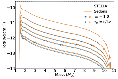
Figure 5: Evolution of density in the M9.3_R433_E1.0_Ni3.0 models. The curves correspond to, from top to bottom, profiles at day 20, 30, 40, 50, 60, 80, and 90. The stars and points mark the locations of the photosphere and where $\tau_{\textrm{R}}=c/4v$, respectively. Assuming homology in Sedona only introduces $\approx$10% relative difference with the full hydrodynamical evolution in STELLA.

3.2 Ejecta Thermal Structures

We now compare the thermodynamical states of the ejecta calculated from the two different codes. Deep in the interior, electron scattering dominates the opacity and traps the radiation. In the absence of radioactive heating, the gas temperature then evolves adiabatically as the ejecta expands. We show the gas temperature evolution of the M9.3_R433_E1.0 model in the left panel of Figure 4. The adiabatic evolution is shown as black dashed lines. Adiabaticity breaks down when the radiative diffusion timescale is comparable to the dynamical time at $\tau\approx c/4v$. The mass coordinate locations $m_{\textrm{c/4v}}$ where $\tau_{\textrm{R}}(m_{\textrm{c/4v}})=\int_{m=m_{\textrm{c/4v}}}^{M_{\textrm{ej}}}\kappa_{\rm R}(r)\rho(r)dr=c/4v$ are denoted by circular points. Below these locations, the adiabatic scaling predicts the temperature evolution. The locations of the photosphere $m_{\textrm{ph}}$, which are defined as $\tau_{\textrm{R}}(m_{\textrm{ph}})=1$, are marked by the star symbols.

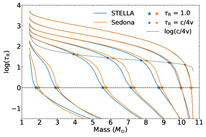
Figure 6: Evolution of the integrated optical depth in the M9.3_R433_E1.0_Ni3.0 model. The curves correspond to, from top to bottom, profiles at day 20, 30, 40, 50, 60, 80, and 90. The stars and points mark the locations of the photosphere and where $\tau_{\textrm{R}}=c/4v$, respectively.

We can also derive a temperature prediction assuming the radioactive energy release (in forms of both gamma-rays and positrons) is locally deposited. Mathematically, we adopted the nuclear energy production rate from Equation (13) of Nadyozhin (1994). On the right panel of Figure 4, such analytical scaling again reproduces the inner ejecta temperature where radiative trapping dominates ($\tau_{\textrm{R}}\geq c/4v$). At $\tau_{\textrm{R}}<c/4v$ (above the circular points), we expect the temperature structures to be modified by the transport of radiation.

To understand the slight offsets of the STELLA and Sedona temperature profiles near the photosphere, we show in Figure 5 the density evolution of the same M9.3_R433_E1.0_Ni3.0 model. While the assumption of homology in Sedona follows the density evolution to within $\approx$10% of STELLA, the residual hydrodynamical acceleration in STELLA after model handoff lowers the overall optical depth. As a result, radiative cooling via diffusive losses is slightly more efficient and the recombination front and photosphere recede deeper into the ejecta. The resultant offsets in the photospheric locations are also illustrated in Figure 6.

A comparison of opacity as a function of gas temperature at the time of handoff is shown in Figure 7 for the M9.3_R433_E1.0_Ni3.0 model. Even though the radiation transport schemes are very different between the codes, the opacity variations they encompass are mostly consistent. The opacity from the default version of STELLA packaged with MESA is also shown – the hydrogen recombination front is bracketed only by two temperature grid points at $\log(T_{\rm gas}/K)$ of 3.8 and 4.0, causing large interpolation errors in between. Nevertheless, this offset in opacity does not introduce significant deviations in the effective temperature, resulting in overall very similar light curves. At $\log(T/K)>4.0$, the difference in opacity can be attributed to the different atomic line lists and analytical expressions for the bound-free and free-free opacity.

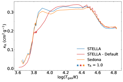
Figure 7: Rosseland mean opacity as a function of gas temperature in the M9.3_R433_E1.0_Ni3.0 model at the moment of model handoff (day 20). The star markers represent the locations of the photosphere. The sawtooth patterns at $\log(T_{\textrm{gas}})\geq 4.4$ are the result of the coarse zone resolution (N${}_{\textrm{reduced}}$ = 50) of the opacity tables in the default version of STELLA.

3.3 Towards Monte Carlo Radiation Hydrodynamics

While the main focus of this work is to verify the reliability of different radiation transport methods in light curve modeling, the Monte Carlo approach of Sedona allows tallying of the radiative moments at almost no additional costs. A comparison of the radiative moments not only informs the robustness of both methods, it also serves as a numerical experiment leading towards multi-dimensional Monte Carlo radiation hydrodynamics.

In the mixed-frame radiation transport formalism of Sedona, the radiation energy density $E_{\textrm{r}}$, radiative flux $F_{\textrm{r}}$, and radiation pressure $P_{\textrm{r}}$ are tracked in the lab frame. In spherical symmetry, non-radial quantities vanish and only the radial components of the radiative flux and pressure are followed. The lab frame quantities are Lorentz-transformed into the co-moving frame quantities $E_{\textrm{r,0}}$, $F_{\textrm{r,0}}$, and $P_{\textrm{r,0}}$ (Mihalas & Weibel-Mihalas, 1999). The profiles of the co-moving frequency-integrated flux factor $F_{\textrm{r,0}}/cE_{\textrm{r,0}}$ are plotted in Figure 8 for the M12.7_R719_E0.84_Ni4.8 model.

In the deep interior of the ejecta, radiation is in the diffusive regime and is nearly isotropic. The net radial flux is therefore small compared to the energy density. In this region, the flux factors computed by the two radiation transport methods agree well with each other, although the MC scheme shows statistical noise. The fluctuation in Sedona’s flux factor originates from the numerical difficulty of representing a near-zero value by the sum of numerous discrete values close in magnitudes but opposite in signs. We also include the analytical predictions based on the Fick’s law of radiative diffusion $F_{\textrm{r,0}}/cE_{\textrm{r,0}}=-(1/3\kappa_{\textrm{R}}\rho)d\ln(E_{\textrm{r,0}})/dr$ as dashed lines, which accurately track the flux factor below the photosphere. The non-monotonicity in the analytical predictions of the STELLA model is the result of discretization errors in computing the $d\ln(E_{\textrm{r,0}})/dr$ term from the spatially varying zone sizes.

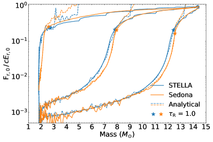
Figure 8: Co-moving frame frequency-integrated flux factor at day 120, 80, and 50 (top to bottom) of the M12.7_R719_E0.84_Ni4.8 model. Locations of the photosphere are marked with the star symbols. The analytical predictions based on Fick’s law of radiative diffusion are plotted as dashed lines.

Near the photosphere, the factor quickly converges to a larger value with a much lower level of MC noise. Above the photosphere, radiation approximates free-streaming and the flux factor approaches unity. In this optically thin region, Fick’s law no longer holds and the analytically predicted flux factor diverges from the true value as expected.

In the diffusion-dominated regime, Roth & Kasen (2015) have proposed a variance-reduction MC flux estimator based on the divergence of radiation pressure, i.e., $F_{\textrm{r,0}}=c\nabla\cdot P_{\textrm{r,0}}/\kappa_{\textrm{R}}\rho\approx c\nabla\cdot E_{\textrm{r,0}}/3\kappa_{\textrm{R}}\rho$. When radiation is isotropic, following the scalar quantity $E_{\textrm{r,0}}$ with discrete photon packets is less prone to statistical noise than tallying the vector quantity $F_{\textrm{r,0}}$. We confirm that this noise reduction estimator reproduces exactly the analytical predictions shown in Figure 8.

We observe that both the STELLA and Sedona models agree well with its Fick’s law predictions deep in the ejecta, and evolve smoothly outward. It shows that the Monte Carlo radiation transport method holds promises in radiation hydrodynamical applications, where the radiative moments can be used as source terms coupled to gas dynamics evolution.

4 Summary

In this work, we conduct the first detailed comparison of the light curves and ejecta structures produced by the moment-based radiation hydrodynamical code STELLA and the particle-based, Monte Carlo radiation transport code Sedona. Radiation transport methods based on radiative moments and discrete photon packets are fundamentally different. With ejecta models derived from realistic progenitor stellar evolution, this comparison serves as an important evaluation of two approaches to radiation transport modeling of supernovae.

During the plateau phase, the light curves generated by the two codes agree to within $\approx$5%. In the late-time radioactive decay phase, the difference is at $\approx$3% level, owing to the different handling choices for the deposition of positron kinetic energy from the cobalt decays. The agreements provide confidence in the fidelity of both codes and radiation transport approaches. Sedona’s homology assumption in evolving the ejecta structures is also found to reproduce the ejecta’s full thermodynamical evolution fairly well. The residual hydrodynamical acceleration in STELLA only induces $\approx$10% differences in the density profiles, and resultant slight offsets in the photospheric locations.

Although Monte Carlo radiation transport is highly adaptable and is not subject to any specific closure relations, a large number of photon packets is required to suppress the statistical noise below an acceptable level. For instance, a typical Sedona run including radioactive decays follows the histories of $\sim$10⁸ photon packets. The high computational demands limit the scope of parameter surveys that are tractable with Sedona. Current progress is being made to break the efficiency barrier by optimizing the radiation transport in the diffusive regime within Sedona.

The flexibility of the Monte Carlo approach to radiation in Sedona also tracks the radiative moments (energy density, flux, and pressure) and verifies the quality of the 1D closure scheme in STELLA. We find that STELLA’s moment method tracks the transition from the minuscule flux in the diffusive regime to the free-streaming flux in the optically thin regime with comparable accuracy to the Monte Carlo approach. The present work demonstrates that it is promising to extend the Monte Carlo framework towards full radiation hydrodynamical simulations.

References

- Andrews et al. (2019) Andrews, J. E., Sand, D. J., Valenti, S., et al. 2019, ApJ, 885, 43
- Baklanov et al. (2005) Baklanov, P. V., Blinnikov, S. I., & Pavlyuk, N. N. 2005, Astronomy Letters, 31, 429
- Baron et al. (1996) Baron, E., Hauschildt, P. H., Nugent, P., & Branch, D. 1996, MNRAS, 283, 297
- Bellm et al. (2019) Bellm, E. C., Kulkarni, S. R., Graham, M. J., et al. 2019, PASP, 131, 018002
- Blinnikov & Sorokina (2004) Blinnikov, S., & Sorokina, E. 2004, Ap&SS, 290, 13
- Blinnikov et al. (1998) Blinnikov, S. I., Eastman, R., Bartunov, O. S., Popolitov, V. A., & Woosley, S. E. 1998, ApJ, 496, 454
- Blinnikov et al. (2006) Blinnikov, S. I., Röpke, F. K., Sorokina, E. I., et al. 2006, A&A, 453, 229
- Burrows et al. (2020) Burrows, A., Radice, D., Vartanyan, D., et al. 2020, MNRAS, 491, 2715
- Clocchiatti & Wheeler (1997) Clocchiatti, A., & Wheeler, J. C. 1997, ApJ, 491, 375
- Davis et al. (2014) Davis, S. W., Jiang, Y.-F., Stone, J. M., & Murray, N. 2014, ApJ, 796, 107
- Dessart & Hillier (2010) Dessart, L., & Hillier, D. J. 2010, MNRAS, 405, 2141
- Dessart & Hillier (2011) —. 2011, MNRAS, 410, 1739
- Dessart & Hillier (2019) —. 2019, A&A, 625, A9
- Dessart et al. (2013) Dessart, L., Hillier, D. J., Waldman, R., & Livne, E. 2013, MNRAS, 433, 1745
- Duffell (2016) Duffell, P. C. 2016, ApJ, 821, 76
- Eastman & Pinto (1993) Eastman, R. G., & Pinto, P. A. 1993, ApJ, 412, 731
- Goldberg & Bildsten (2020) Goldberg, J. A., & Bildsten, L. 2020, arXiv e-prints, arXiv:2005.07290
- Goldberg et al. (2019) Goldberg, J. A., Bildsten, L., & Paxton, B. 2019, ApJ, 879, 3
- Gronenschild & Mewe (1978) Gronenschild, E. H. B. M., & Mewe, R. 1978, A&AS, 32, 283
- Heger et al. (2003) Heger, A., Fryer, C. L., Woosley, S. E., Langer, N., & Hartmann, D. H. 2003, ApJ, 591, 288
- Hunter (2007) Hunter, J. D. 2007, Computing in Science & Engineering, 9, 90
- Janka et al. (2016) Janka, H.-T., Melson, T., & Summa, A. 2016, Annual Review of Nuclear and Particle Science, 66, 341
- Jones et al. (2001–) Jones, E., Oliphant, T., Peterson, P., et al. 2001–, SciPy: Open source scientific tools for Python, , . http://www.scipy.org/
- Junde et al. (2011) Junde, H., Su, H., & Dong, Y. 2011, Nuclear Data Sheets, 112, 1513
- Karp et al. (1977) Karp, A. H., Lasher, G., Chan, K. L., & Salpeter, E. E. 1977, ApJ, 214, 161
- Kasen et al. (2006) Kasen, D., Thomas, R. C., & Nugent, P. 2006, ApJ, 651, 366
- Kasen & Woosley (2009) Kasen, D., & Woosley, S. E. 2009, ApJ, 703, 2205
- Kluyver et al. (2016) Kluyver, T., Ragan-Kelley, B., Pérez, F., et al. 2016, in Positioning and Power in Academic Publishing: Players, Agents and Agendas, ed. F. Loizides & B. Schmidt, IOS Press, 87 – 90
- Kochanek et al. (2017) Kochanek, C. S., Shappee, B. J., Stanek, K. Z., et al. 2017, PASP, 129, 104502
- Kozyreva et al. (2019) Kozyreva, A., Nakar, E., & Waldman, R. 2019, MNRAS, 483, 1211
- Kozyreva et al. (2017) Kozyreva, A., Gilmer, M., Hirschi, R., et al. 2017, MNRAS, 464, 2854
- Krumholz & Thompson (2012) Krumholz, M. R., & Thompson, T. A. 2012, ApJ, 760, 155
- Kurucz & Bell (1995) Kurucz, R. L., & Bell, B. 1995, Atomic line list
- Li et al. (2011) Li, W., Leaman, J., Chornock, R., et al. 2011, MNRAS, 412, 1441
- LSST Science Collaboration et al. (2009) LSST Science Collaboration, Abell, P. A., Allison, J., et al. 2009, arXiv e-prints, arXiv:0912.0201
- Martinez & Bersten (2019) Martinez, L., & Bersten, M. C. 2019, A&A, 629, A124
- Meza & Anderson (2020) Meza, N., & Anderson, J. P. 2020, arXiv e-prints, arXiv:2002.01015
- Mihalas & Klein (1982) Mihalas, D., & Klein, R. I. 1982, Journal of Computational Physics, 46, 97 . http://www.sciencedirect.com/science/article/pii/0021999182900079
- Mihalas & Weibel-Mihalas (1999) Mihalas, D., & Weibel-Mihalas, B. 1999, Foundations of Radiation Hydrodynamics, Dover Books on Physics (Dover Publications). https://books.google.com/books?id=f75C_GN9KZwC
- Moriya et al. (2018) Moriya, T. J., Sorokina, E. I., & Chevalier, R. A. 2018, Space Sci. Rev., 214, 59
- Morozova et al. (2016) Morozova, V., Piro, A. L., Renzo, M., & Ott, C. D. 2016, ApJ, 829, 109
- Morozova et al. (2015) Morozova, V., Piro, A. L., Renzo, M., et al. 2015, ApJ, 814, 63
- Nadyozhin (1994) Nadyozhin, D. K. 1994, ApJS, 92, 527
- Oliphant (2006) Oliphant, T. E. 2006, A guide to NumPy, Vol. 1 (Trelgol Publishing USA)
- Paxton et al. (2011) Paxton, B., Bildsten, L., Dotter, A., et al. 2011, ApJS, 192, 3
- Paxton et al. (2013) Paxton, B., Cantiello, M., Arras, P., et al. 2013, ApJS, 208, 4
- Paxton et al. (2015) Paxton, B., Marchant, P., Schwab, J., et al. 2015, ApJS, 220, 15
- Paxton et al. (2018) Paxton, B., Schwab, J., Bauer, E. B., et al. 2018, ApJS, 234, 34
- Paxton et al. (2019) Paxton, B., Smolec, R., Schwab, J., et al. 2019, ApJS, 243, 10
- Pinto & Eastman (2000) Pinto, P. A., & Eastman, R. G. 2000, ApJ, 530, 757
- Popov (1993) Popov, D. V. 1993, ApJ, 414, 712
- Rosdahl & Teyssier (2015) Rosdahl, J., & Teyssier, R. 2015, MNRAS, 449, 4380
- Roth & Kasen (2015) Roth, N., & Kasen, D. 2015, ApJS, 217, 9
- Smartt (2015) Smartt, S. J. 2015, PASA, 32, e016
- Smartt et al. (2009) Smartt, S. J., Eldridge, J. J., Crockett, R. M., & Maund, J. R. 2009, MNRAS, 395, 1409
- Smith et al. (2011) Smith, N., Li, W., Filippenko, A. V., & Chornock, R. 2011, MNRAS, 412, 1522
- Sukhbold et al. (2016) Sukhbold, T., Ertl, T., Woosley, S. E., Brown, J. M., & Janka, H. T. 2016, ApJ, 821, 38
- Swartz et al. (1995) Swartz, D. A., Sutherland, P. G., & Harkness, R. P. 1995, ApJ, 446, 766
- Takáts et al. (2015) Takáts, K., Pignata, G., Pumo, M. L., et al. 2015, MNRAS, 450, 3137
- Tsang & Milosavljević (2015) Tsang, B. T. H., & Milosavljević, M. 2015, MNRAS, 453, 1108
- Utrobin et al. (2017) Utrobin, V. P., Wongwathanarat, A., Janka, H. T., & Müller, E. 2017, ApJ, 846, 37
- Van Dyk et al. (2012a) Van Dyk, S. D., Davidge, T. J., Elias-Rosa, N., et al. 2012a, AJ, 143, 19
- Van Dyk et al. (2012b) Van Dyk, S. D., Cenko, S. B., Poznanski, D., et al. 2012b, ApJ, 756, 131
- Vartanyan et al. (2019) Vartanyan, D., Burrows, A., & Radice, D. 2019, MNRAS, 489, 2227
- Verner et al. (1993) Verner, D., Yakovlev, D., Band, I., & Trzhaskovskaya, M. 1993, Atomic Data and Nuclear Data Tables, 55, 233 . http://www.sciencedirect.com/science/article/pii/S0092640X83710223
- Verner et al. (1996) Verner, D. A., Verner, E. M., & Ferland, G. J. 1996, Atomic Data and Nuclear Data Tables, 64, 1
- Wheeler et al. (2015) Wheeler, J. C., Johnson, V., & Clocchiatti, A. 2015, MNRAS, 450, 1295
- Wilk et al. (2019) Wilk, K. D., Hillier, D. J., & Dessart, L. 2019, MNRAS, 487, 1218
- Wongwathanarat et al. (2015) Wongwathanarat, A., Müller, E., & Janka, H. T. 2015, A&A, 577, A48
- Woosley & Heger (2007) Woosley, S. E., & Heger, A. 2007, Phys. Rep., 442, 269
- Woosley et al. (2002) Woosley, S. E., Heger, A., & Weaver, T. A. 2002, Reviews of Modern Physics, 74, 1015
- Woosley & Weaver (1995) Woosley, S. E., & Weaver, T. A. 1995, ApJS, 101, 181
- Zhang & Davis (2017) Zhang, D., & Davis, S. W. 2017, ApJ, 839, 54
- Zhang & Sutherland (1994) Zhang, X.-H., & Sutherland, P. 1994, ApJ, 422, 719