OSSOS XX: The Meaning of Kuiper Belt Colors

Abstract

Observations show that 100-km-class Kuiper belt objects (KBOs) can be divided in (at least) two color groups, hereafter red (R; $g-i<1.2$) and very red (VR; $g-i>1.2$), reflecting a difference in their surface composition. This is thought to imply that KBOs formed over a relatively wide range of radial distance, $r$. The cold classicals at $42<r<47$ au are predominantly VR and known Neptune Trojans at $r\simeq 30$ au are mostly R. Intriguingly, however, the dynamically hot KBOs show a mix of R and VR colors and no correlation of color with $r$. Here we perform migration/instability simulations where the Kuiper belt is populated from an extended planetesimal disk. We find that the color observations can be best understood if R objects formed at $r<r^{*}$ and VR objects at $r>r^{*}$, with $30<r^{*}<40$ au. The proposed transition at $30<r^{*}<40$ au would explain why the VR objects in the dynamically hot population have smaller orbital inclinations than the R objects, because the orbital excitation from Neptune weakens for orbits starting beyond 30 au. Possible causes of the R-VR color bimodality are discussed.

1 Introduction

The vast majority of KBOs are too faint for spectroscopic observations, but their surface composition can be studied with broadband photometry. Photometric observations indicate that the color distribution of KBOs is bimodal with red (R; defined as $g-i<1.2$ in Wong & Brown (2017); observations made in the $ugriz$ magnitude system) and very red (VR; $g-i>1.2$) classes (e.g., Luu & Jewitt 1996, 1998; Tegler & Romanishin 1998, 2000; Jewitt & Luu 1998, 2001; Peixinho et al. 2003, 2008, 2012, 2015; Tegler et al. 2003, 2016; Barucci et al. 2005; Sheppard 2012; Fraser & Brown 2012; Wong & Brown 2017; Pike et al. 2017; Jewitt 2018; Schwamb et al. 2019, Marsset et al. 2019). Known Neptune Trojans at radial distance $r\simeq 30$ au are R (Sheppard & Trujillo 2006, Parker et al. 2013, Jewitt 2018), with one known exception (2013 VX30; Lin et al. 2019), and most classified cold classicals (CCs) with semimajor axes $42<a<47$ au are VR. This has been taken as evidence that colors have something to do with the distance at which different objects formed. Confusing matters, however, the dynamically hot populations with $30<a<50$ au show a mix of R and VR colors, and there does not appear to be any obvious correlation of colors with $r$ (e.g., Peixinho et al. 2015, Marsset et al. 2019).

Brown et al. (2011) proposed that the early surface compositions of KBOs were set by volatile evaporation after the objects formed. A strong gradient in surface composition, coupled with UV irradiation and particle impacts, then presumably led to the surface colors that we see today. For example, the sublimation line of (pure) ammonia, NH₃, is near 34 au (Brown et al. 2011). Objects formed at the current location of CCs may therefore uniquely retain NH₃, which has been shown to affect irradiation chemistry and could plausibly lead to the VR colors of these objects. But how to interpret the R colors of Neptune Trojans and the bimodal distribution of colors in the hot population?

Neptune Trojans were presumably trapped as co-orbitals during Neptune’s migration (e.g., Nesvorný & Vokrouhlický 2009, Parker 2015, Gomes & Nesvorný 2016). Their inferred formation location is $r\simeq 25$-30 au. The predominantly R colors of Neptune Trojans (Jewitt 2018, Lin et al. 2019) would thus be hard to understand if the R to VR transition is related the sublimation line of the hydrogen sulfide ice (H₂S, $r\simeq 15$-20 au), as suggested by Wong & Brown (2016, 2017). Instead, the R colors of Neptune Trojans seem to imply that the transition occurred farther out, probably beyond $\sim$30 au. This reasoning leads to an impasse, however, because our best dynamical models suggest that the dynamically hot KBOs were implanted onto their current orbits from the massive planetesimal disk inside of $30$ au. Their colors should thus be uniformly R, just like Neptune Trojans, but they are not.

2 Color Hypothesis

Here we examine the possibility that the hot populations (i.e., HCs, Plutinos, SDOs) in the present-day Kuiper belt are a mix of bodies implanted from the massive disk below 30 au (source of R) and the low-mass disk extension beyond 30 au (source of VR). On one hand, the surface density of planetesimals must have been quite low at $r>30$ au for Neptune to stop at 30 au (Gomes et al. 2004, Nesvorný 2018). The outer disk extension thus represents a smaller source reservoir than the massive disk below 30 au. On the other hand, the chances to evolve from 30-40 au onto a dynamically hot orbit in the Kuiper belt are better (e.g., Hahn & Malhotra 2005). It is thus plausible that a good share of hot KBOs come from the 30-40 au region.

The proposed color transition at $r^{*}>30$ au could explain why the VR objects in the dynamically hot population have smaller orbital inclinations than the R objects (e.g., Tegler & Romanishin 2000; Trujillo & Brown 2002; Hainaut & Delsanti 2002; Peixinho et al. 2008, 2015; Marsset et al. 2019), because the orbital excitation from Neptune is expected to weaken for orbits starting beyond 30 au. We investigate this issue in detail in Section 4.3. In contrast, no such correlation would be expected if both the R and VR objects started below 30 au, where Neptune’s gravitational effects are uniformly strong (Nesvorný 2015a).

If some of the R objects can be pushed out from $r<r^{*}$ into the CC population, this could explain the “blue” CC binaries reported in Fraser et al. (2017) and indicate that $r^{*}>35$ au. Note that the analysis presented here aims at explaining the global distribution of KBO colors, including the color-inclination correlation; this is well beyond the scope of the analysis of blue binaries in Fraser et al. (2017). Our color hypothesis would also be consistent with the R colors of Jupiter Trojans (Emery et al. 2015) and irregular satellites of the giant planets (Graykowski & Jewitt 2018), because they are thought to be captured from the massive disk below 30 au, and thus expected to be R.

Pike et al. (2017) pointed out that cold and hot KBOs with $g-r>0.8$ (roughly the VR category here) have different $r-z$ colors (hot VR KBOs exhibit redder $r-z$ colors). This was used in Schwamb et al. (2019) to propose that the original planetesimal disk had two color transitions: one at $\sim$33 au, from VR with redder $r-z$ colors to R (called “neutral” in Schwamb et al.) and another one at $\sim$39 au, from R to VR with bluer $r-z$ colors. This cannot work, however, because: (i) it would not fit the predominantly R colors of Neptune Trojans (Jewitt 2018, Lin et al. 2019), and (ii) VR objects starting below 33 au would end up on orbits with higher orbital inclinations than R objects starting at 33-39 au (Section 4.3), which is opposite to what the color observations indicate (e.g., Marsset et al. 2019). Pike et al.’s result is more likely related to a change of $r-z$ with original orbital radius from $r^{*}$ to the location of CCs at $r>42$ au.

3 Methods

The occurrence of R and VR objects in each KBO category can be determined, in the context of the suggested model, from the initial disk profile (massive at $r<30$ au with decreasing surface density beyond 30 au), the radial distance $r^{*}$ which marked the original transition from R to VR colors, and the implantation probability from $r$ to a specific dynamical class. This is the main goal of the work presented here. We aim at identifying the disk profiles and the range of $r^{*}$ values that best fit the existing color data.

3.1 Integration Method

The numerical integrations conducted here consist of tracking the orbits of four giant planets (Jupiter to Neptune) and a large number of particles ($2\times 10^{6}$) representing the original trans-Neptunian disk. To set up an integration, Uranus and Neptune are placed inside of their current orbits and migrated outward. The swift_rmvs4 code, part of the Swift $N$-body integration package (Levison & Duncan 1994), is used to follow the orbits of planets and massless disk particles. The code was modified to include additional forces that mimic the radial migration and damping of planetary orbits. These forces are parametrized by the exponential e-folding timescale, $\tau$.

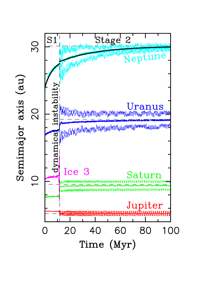
The migration histories of planets are informed by our best models of planetary migration/instability (Nesvorný & Morbidelli 2012, hereafter NM12; also see Deienno et al. 2017). In the NM12 models, Neptune’s migration can be divided into two stages separated by a brief episode of dynamical instability (jumping Neptune model, Figure 1). Neptune migrates on a circular orbit before the instability (Stage 1). Its eccentricity becomes excited during the instability and is subsequently damped by a gravitational interaction with disk planetesimals (Stage 2). The instability is needed, among other things (e.g., orbital eccentricity of Jupiter, asteroid belt constraints; Nesvorný 2018), to explain the Kuiper belt kernel near 44 au (Section 4.2; Petit et al. 2011, Nesvorný 2015b, Bannister et al. 2018).

The orbital behavior of Neptune during the first and second migration stages can be approximated by $\tau_{1}\simeq 5$-30 Myr and $\tau_{2}\simeq 30$-100 Myr. We find that Neptune’s migration in a power-law radial disk profile is often too fast ($\tau_{1}<10$ Myr) to satisfy the inclination constraint and it is difficult to fine-tune the total disk mass, $M_{\rm disk}$, to obtain $\tau_{1}\gtrsim 10$ Myr. The power-law disks also efficiently damp Neptune’s eccentricity during Stage 2, which effects the ability of Neptune’s resonances to implant bodies on the high-inclination orbits in the Kuiper belt (Volk & Malhotra 2019). The exponential disks show more promising results (e.g., $\tau_{1}=12$ Myr and $\tau_{2}=27$ Myr in Fig. 1). We account for the jitter that Neptune’s orbit experiences due to close encounters with Pluto-class objects. Neptune’s grainy migration is important to produce the right proportion of resonant and non-resonant KBOs (Nesvorný & Vokrouhlický 2016).

All migration simulations are run to 0.5 Gyr. They are extended to 4.5 Gyr with the standard swift_rmvs4 code (i.e., without migration/damping after 0.5 Gyr). We perform four new simulations in total (Table 1). In the first case, we adopt $\tau_{1}=10$ Myr and $\tau_{2}=30$ Myr as indicated by Fig. 1. This case roughly corresponds to the shortest migration timescale that is required to satisfy the inclination constraint (Nesvorný 2015a; but see Volk & Malhotra 2019). In the second case, we use longer timescales: $\tau_{1}=30$ Myr and $\tau_{2}=100$ Myr. This case would correspond to a slower migration driven by a lower mass planetesimal disk. A very slow migration of Neptune during the second stage would be needed, for example, to explain Saturn’s obliquity (Ward & Hamilton 2004, Hamilton & Ward 2004, Vokrouhlický & Nesvorný 2015). These two cases bracket the interesting range of possibilities. We perform two simulations in each case, one with Neptune’s jump at the transition from Stages 1 to 2 (Nesvorný 2015b) and one without it. The jump is implemented as an instantaneous increase of Neptune’s semimajor axis by 0.4-0.5 au (Table 1). In the following text, the simulations without jump are labeled s10/30 and s30/100; the ones with jump are s10/30j and s30/100j.

The final orbits of Uranus and Neptune are fine-tuned in these simulations such as the period ratio $P_{\rm N}/P_{\rm U}=1.92$-1.95, where $P_{\rm U}$ and $P_{\rm N}$ are the orbital periods of Uranus and Neptune (Table 1). The orbital ratio of the real planets in the current Solar System is $P_{\rm N}/P_{\rm U}=1.96$. We opt for having model $P_{\rm N}/P_{\rm U}$ a tiny bit smaller than 1.96 to make sure that Uranus and Neptune are never too close to the 2:1 resonance (the effects of the 2:1 resonance can disrupt the Kuiper belt structure, change stability of resonant populations, etc.). We also make sure that the final semimajor axes, eccentricities and inclinations of planets are as close to the real values as possible. Neptune’s orbital eccentricity is assumed to increase to $e_{\rm N}=0.1$ at the transition from Stage 1 to Stage 2, at often seen in our self-consistent instability simulations (Fig. 1). The damping routines are tuned such that the simulated orbit of Neptune ends with just the right orbital inclination and eccentricity (current mean $e_{\rm N}=0.009$). The cases with larger final $e_{\rm N}$, such as the ones described as Case A in Volk & Malhotra (2019), are not investigated here.

3.2 Planetesimal Disk

Previous studies of planetary migration/instability often adopted a two-part disk structure with a massive planetesimal disk on the inside, a low-mass disk on the outside, and a sharp transition from high to low surface densities near 30 au. The inner part of the planetesimal disk, from just outside Neptune’s initial orbit to $\sim$30 au, was estimated mass to be $M_{\rm disk}\simeq 15$-20 $M_{\rm Earth}$ (NM12, Nesvorný et al. 2013, 2019; Deienno et al. 2017). It was argued that the massive disk must have been truncated at $\sim$30 au for Neptune to stop at 30 au (e.g., Gomes et al. 2004). Our tests show that the disk truncation is not required (Fig. 1). In fact, Neptune may have ended at $\simeq$30 au just because the planetesimal surface density at $\gtrsim$30 au was subcritical (Neptune stops if the density is below 1-1.5 $M_{\rm Earth}$ au^-1; Nesvorný 2018). In other words, Neptune’s current orbit does not constrain the radial gradient of the planetesimal surface density near 30 au. Instead, it just tells us that the surface density was low beyond 30 au.

Another constraint on the surface density profile beyond 30 au can be inferred from the CC population. The mass of CCs was estimated to be $M_{\rm CC}\sim 3\times 10^{-4}$ $M_{\rm Earth}$ in Fraser et al. (2014) but we find $M_{\rm CC}=(3\pm 2)\times 10^{-3}$ $M_{\rm Earth}$ from OSSOS (Outer Solar System Origins Survey; Appendix A). The difference is caused, at least in part, by different observational datasets used for the analyses (OSSOS biases are carefully characterized) and different magnitude distribution assumptions (we use an exponentially tampered size distribution in Appendix A). Nesvorný (2015b) found that this represents only a fraction of the original population of planetesimals at 45 au. Adopting our OSSOS estimate, we can therefore very roughly estimate that the original disk mass density at 45 au was $\sim 10^{-3}$ $M_{\rm Earth}$ au^-1. Together, the two constraints discussed above imply a strong surface density gradient from 30 au to 45 au. For example, if the linear mass density of the planetesimal disk followed $\exp[-(r-24\,{\rm au})/\Delta r]$, then $\Delta r\sim 2.5$ au. This is consistent with the total mass and radial profile of the planetesimal disk that we used for Figure 1.

Here we examine three disk profiles: the (1) truncated power-law (surface density $\Sigma\propto 1/r^{\gamma}$ with $\gamma=1$-2, truncated at 30 au, a low-mass extension beyond 30 au; Fig. 2a), (2) exponential ($\Sigma\propto\exp[(r-r_{0})/\Delta r]/r$, where $r_{0}$ is the inner edge radius near $\sim$24 au, and $\Delta r$ is one e-fold, no outer truncation here; Fig. 2b), and (3) hybrid profiles (power law $\Sigma\propto 1/r^{\gamma}$ below 28 au, exponential above 28 au; Fig. 2c). Each of our simulations includes two million disk planetesimals distributed from outside Neptune’s initial orbit at $\sim$24 au to $>$50 au (one million at $<30$ au and one million at $>30$ au). Such a large number of bodies is needed to obtain good statistics. The initial eccentricities and inclinations of planetesimals are set according to the Rayleigh distribution with $\sigma_{e}=0.1$ and $\sigma_{i}=0.05$. The planetesimals are assumed to be massless, such that their gravity does not interfere with the code’s migration/damping routines.

We use weights to set up the three profiles in Fig. 2. Specifically, the planetesimals starting at orbital radius $r$ are given weight $w(r)$, where $w(r)$ follows the selected initial density profile. The weights are propagated through the simulation and analysis, and used to gauge the contribution of each particle to the model results, including the color ratios reported in Sect. 4.3. For the truncated power-law profile in Fig. 2a, the step in the surface density at 30 au is parametrized by the contrast parameter, $c$, which is simply the ratio of densities on either side of 30 au. The exponential and hybrid disks in Figs. 2b and c are parametrized by one e-fold $\Delta r$. To match the constraints described above, $\Delta r$ of the hybrid disk must be smaller than $\Delta r$ of the exponential disk. We assign a color to each simulated object depending on whether it started at $r<r^{*}$ or $r>r^{*}$. The color transition at $r^{*}$ is assumed to be a sharp boundary between R and VR.

3.3 Comparison with observations

We use the OSSOS detection simulator (Bannister et al. 2018) to show that our model results are roughly consistent with the orbital structure of the Kuiper belt. A more systematic comparison will be published elsewhere as part of the OSSOS publication series. OSSOS is the largest Kuiper belt survey with published characterization (1142 ensemble detections; Bannister et al. 2018). The simulator was developed by the OSSOS team to aid the interpretation of their observations. Given intrinsic orbital and magnitude distributions, the OSSOS simulator returns a sample of objects that would have been detected by the survey, accounting for flux biases, pointing history, rate cuts and object leakage (Lawler et al. 2018).

In this work, we input our model results into the OSSOS simulator to compute the detection statistics. We first increase the statistics by performing a 10-Myr integration starting from $t=4.5$ Gyr. The orbital elements of planets and model KBOs are saved with the $10^{5}$ yr cadence (generating 100 outputs for each body). For each output, we rotate the reference system such that Neptune appears near Neptune’s current position on the sky. This assures a consistency with the OSSOS observations. The OSSOS simulator then reads the orbital elements of model KBOs on input.

The input magnitudes/sizes of KBOs are modeled as broken power-law distributions (e.g., Fraser et al. 2014). If the original massive disk is really the main source of all dynamically hot populations in the Kuiper belt, their size distributions should be similar and should reflect the size distribution of the disk at the time of its dispersal by Neptune. This is because the collisional evolution in the present-day Kuiper belt is modest and has not altered the size distribution in the size range of KBOs detected by OSSOS (e.g., Nesvorný & Vokrouhlický 2019, their Fig. 12). In more detail, the size distribution can be informed from Jupiter Trojans because Jupiter Trojans were presumably captured at 5.2 au from the same source (e.g., Morbidelli et al. 2005, Nesvorný et al. 2013; but see Pirani et al. 2019), their size distribution has not evolved after capture (Nesvorný et al. 2018) and is well characterized from observations down to diameters $D\simeq 5$ km (Wong & Brown 2015, Yoshida & Terai 2017).

Specifically, we use the cumulative size distribution $N(>\!\!D)=N_{\rm break}(D/D_{\rm break})^{-q_{\rm big}}$ for $D>D_{\rm break}$, where $D_{\rm break}$ is the location of the break, $N_{\rm break}$ is the number of bodies with $D>D_{\rm break}$, and $N(>\!\!D)=N_{\rm break}(D/D_{\rm break})^{-q_{\rm small}}$ for $D<D_{\rm break}$. From observations of Jupiter Trojans and KBOs we set $D_{\rm break}\simeq 100$ km, $q_{\rm small}\simeq 2$ and $q_{\rm big}\simeq 5$. We normalize $N_{\rm break}$ such that the whole planetesimal disk corresponds to 15-20 $M_{\rm Earth}$. This gives $N_{\rm break}\sim 6\times 10^{7}$ bodies with a factor of $\sim$2 uncertainty (mainly due to the uncertain bulk density of Jupiter Trojans and KBOs). The size distribution of planetesimals beyond 40 au is discussed in Appendix A. For simplicity, we use the same albedo $p_{\rm V}=0.1$ for all populations to convert between size and absolute magnitude.

Once we make sure that the simulation results are roughly consistent with the number and orbital distribution of KBOs (Sections 4.1 and 4.2), we proceed by comparing them with the color data (Section 4.3). For that, we use the color database of Peixinho et al. (2015) (publicly available at
http://vizier.cfa.harvard.edu/), the color survey results of Wong & Brown (2017) (356 objects, data available from authors), published data from the Col-OSSOS survey (Pike et al. 2017, Schwamb et al. 2019, Marsset et al. 2019), and the Neptune Trojan data from Jewitt (2018) and Lin et al. (2019).

The results for each disk profile and $r^{*}$ are compared with the observations discussed above. Specifically, we require that: (1) at least $\sim$90% of Neptune Trojans end up to be R (the best estimate of the intrinsic VR/R ratio of Neptune Trojans, $\sim$0.06 from Lin et al. 2019, has a large statistical uncertainty), (2) over $\sim$90% of CCs end up to be VR (to reflect the predominantly VR colors among CCs), and (3) the VR/R ratio of dynamically hot KBOs (HCs, Plutinos, SDOs) obtained in the model matches the VR/R ratio inferred from observations (intrinsic VR/R $\sim 0.1$-0.3; Wong & Brown 2017, Schwamb et al. 2019). The color distribution is reported here for $D>100$ km objects (absolute magnitudes $H<8.1$ for $p_{\rm V}=0.1$). Changes of the color ratio with size are not investigated here. Special attention is given to the correlation of colors with orbital inclination (e.g., Peixinho et al. 2008, Marsset et al. 2019), which is the chief supporting argument for our color hypothesis (Section 4.3).

3.4 Model caveats

Here we adopt a numerical model with disk planetesimals that do not carry any mass. Neptune’s migration in the planetesimal disk is mimicked by artificial forces. This is not ideal for several reasons. For example, this means that the precession frequencies of planets are not affected by the disk torques in our simulations, while in reality they were (Batygin et al. 2011). The direct gravitational effect of the fifth giant planet (NM12) on the disk planetesimals is also ignored. These additional effects, which may influence the orbital structure of the Kuiper belt, are studied elsewhere (Nesvorný et al., in preparation).

The weighting scheme described in Sect. 3.2 is used to investigate the effect of different radial profiles of the planetesimal disk on the orbital and color distributions of KBOs. This scheme can strictly be applied only to the outer part of the disk beyond 30 au. For $r<30$ au, the radial disk profile is tied to Neptune’s migration, and changing the profile would mean that the character of Neptune’s migration would change as well. Given the high computational expense of these calculations, however, we are unable to resolve this dependence in full detail. So, we do the next best thing, which is to use the weighting scheme to capture the dependence on the source material initially available at different orbital radii, and different migration cases to capture the dependence on the nature of Neptune’s migration. The development of a more self-consistent model that would account for coupling between these effects is left for future work.

Ideally, we would like to have a large suite of dynamical models with different migration timescales, different histories of Neptune’s orbit (Volk & Malhotra 2019), etc., and choose the best model by formally fitting the OSSOS dataset. This would also help to establish the uncertainty of model parameters. Such a systematic exploration of model parameters, however, is not possible with only four dynamical models available to us (Table 1). Here we therefore focus on establishing trends with different parameters in an attempt to roughly triangulate the interesting range of possibilities. The main goal of these efforts is to demonstrate the plausibility of the color hypothesis proposed in Sect. 2.

4 Results

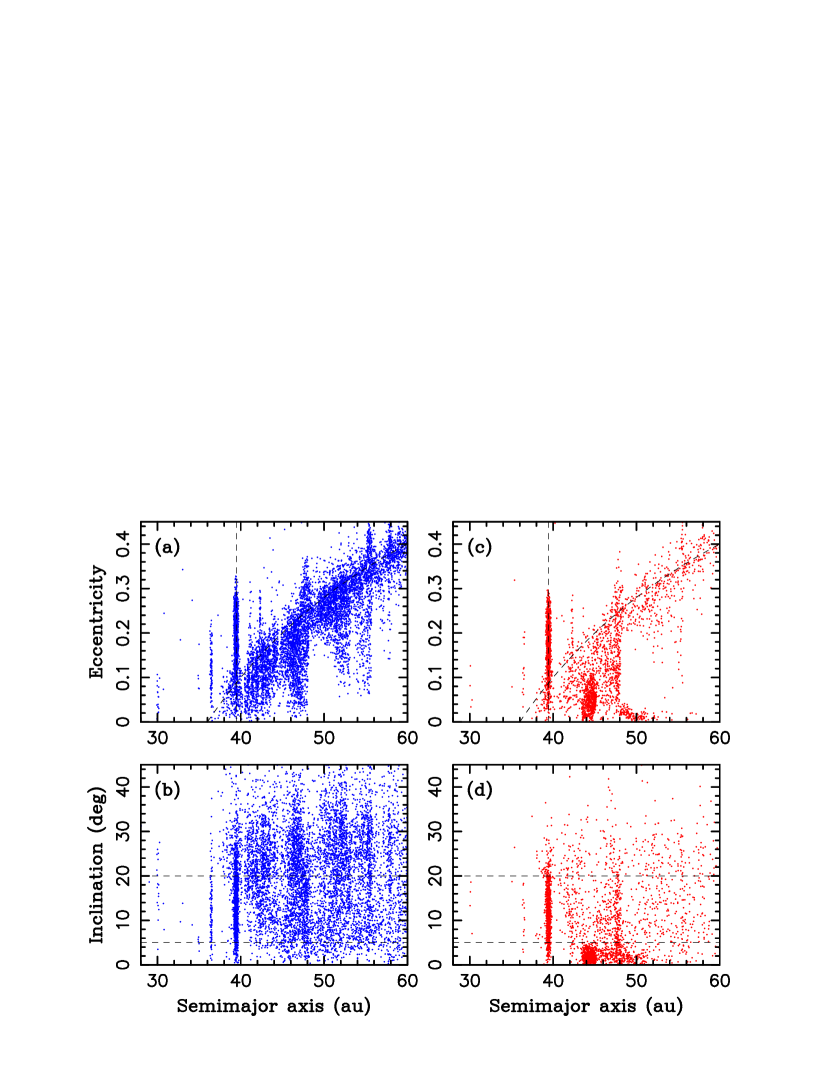
The raw orbital distribution of bodies implanted into the Kuiper belt ($t=4.5$ Gyr) is shown in Figure 3. Note that the raw distribution should not be directly compared to observations because: it (1) does not account for observational biases and (2) corresponds to disk profile with $w(r)=1$ for all $r$ (which is unphysical; e.g., too much emphasis is given to bodies starting with $r>30$ au). We show these plots to illustrate a typical result of our simulations. There are several notable features. The resonant populations, including Neptune Trojans, Plutinos and objects in the 4:3, 2:1 and 5:2 resonances can clearly be identified. Interestingly, the planetesimals sourced from $r<35$ au tend to evolve to higher orbital inclinations than the ones from $r>35$ au (compare panels (b) and (d) in Fig. 3). We interpret this trend as a consequence of weakening of Neptune’s gravitational perturbations with $r$ and use it to discuss the color-inclination correlation in Sect. 4.3.

Another prominent feature in Fig. 3c,d is the concentration of bodies with $a\simeq 44$ au, $e<0.1$ and $i<5^{\circ}$. The concentration appears in the simulation when planetesimals starting at $\sim$40-43 au are captured into the 2:1 resonance with Neptune and subsequently released from the resonance during Neptune’s jump. The slow migration of Neptune’s 2:1 resonance after the jump depletes the cold population beyond 45 au. Results similar to these were used in Nesvorný (2015b) to explain the Kuiper belt kernel (Petit et al. 2011). We will discuss the kernel in more detail in Sect. 4.2. Here we just note that models with a continuous migration of Neptune (i.e., no jump) produce a dispersed orbital distribution of CCs and no kernel.

4.1 Number of KBOs

The number of bodies in different Kuiper belt populations has been determined from observations. Petit et al. (2011) estimated that there should be $35,000\pm 8,000$ HCs with $D>100$ km. Gladman et al. (2012) found that the population of Plutinos in the 3:2 resonance represents $\sim$1/3 of the HC population. From this we have $\sim$12,000 Plutinos with $D>100$ km. Petit et al. (2011) also estimated that there should be $\sim$95,000 CCs with $D>100$ km, but such a large population would be at odds with Fraser et al. (2014), who found that the total mass of CCs represents only $\sim$0.03 of the HC population mass. We find $\simeq$15,000 CCs with $D>100$ km from OSSOS (Appendix A). Finally, Lin et al. (2018) estimated from the Deep Ecliptic Survey that there should be $\simeq$160 Neptune Trojans with absolute magnitude $H<10$ ($D>50$ km for albedo $p_{\rm V}=0.07$) in the $L_{4}$ point. Assuming that the $L_{5}$ population is similar and approximately re-scaling to $D>100$ km, we find that there should be $\sim$100 Neptune Trojans with $D>100$ km. If so, the population of Neptune Trojans (NTs) would be roughly four times larger than the population of Jupiter Trojans.

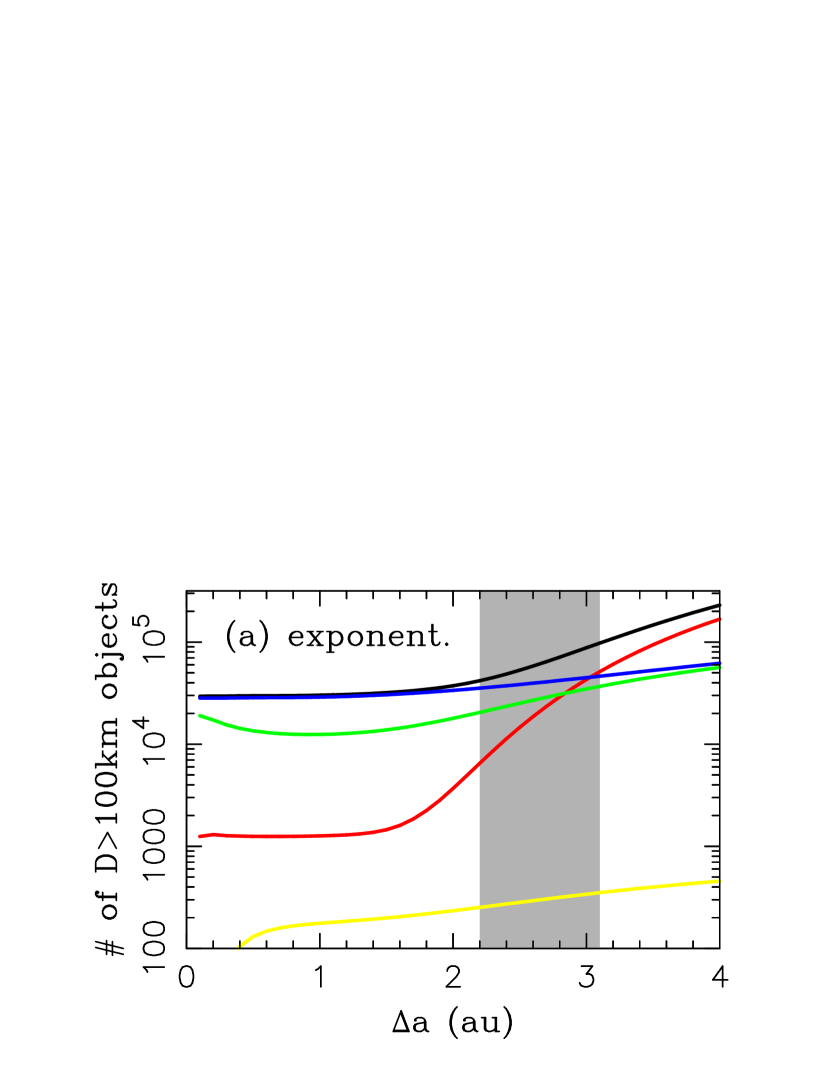
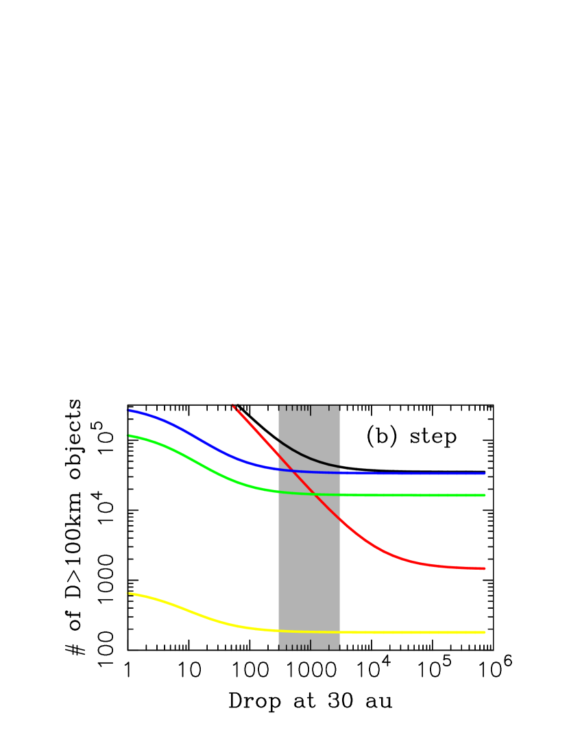
We now address the question of how well the migration models investigated in this work reproduce the inferred number of objects in different populations. The s30/100j simulation yields reasonable results (Fig. 4). Some of the best results are obtained in this case with the exponential profile and $\Delta r=2.5$ au, where we identify 40,000 HCs, 25,000 Plutinos, 15,000 CCs and 300 NTs with $D>100$ km (here we assume that the original disk contained $6\times 10^{7}$ $D>100$ km planetesimals; Nesvorný 2018). The s30/100j simulation with the step profile works as well. Specifically, with $c=1000$, we obtain 35,000 HCs, 20,000 Plutinos, 20,000 CCs and 200 NTs with $D>100$ km, which is practically the same result as for the best exponential profile discussed above. The hybrid disk profiles yield intermediate results and we do not highlight them here.

The s30/100 model (no jump) does not work with the exponential and hybrid profiles. This is because in both these cases, $\Delta r>2$ au is needed to obtain a roughly correct number of CCs. But $\Delta r>2$ au also gives a very large number of Plutinos, both in the absolute ($>$70,000 bodies with $D>100$ km) and relative terms (the Plutino population ends up to be larger than the HC population). This is a consequence of the 3:2 resonance sweeping and efficient capture of planetesimals from $r\simeq 32$-39 au (Hahn & Malhotra 2005). The truncated power-law profile can be used to resolve this problem. Indeed, with $c=1000$, we obtain 40,000 HCs, 25,000 Plutinos, 15,000 CCs and 450 NTs with $D>100$. This is identical to the s30/100j case with $\Delta r=2.5$ au, except that there are $\sim$1.5 times more NTs in s30/100. We do not consider this to be a problem because the population of NTs is very sensitive to details of Neptune’s migration history (e.g., Gomes & Nesvorný 2016).

The s10/30 (no jump) model gives results that are much less compatible with the structure of the Kuiper belt than the results discussed above. This applies independently of the assumed radial profile. For example, with the truncated power-law profile and any value of $c$, the s10/30 model gives an excessive number of HCs (over 80,000 with $D>100$ km), Plutinos (over 60,000) and NTs (over 2,000). We do not include the s10/30 model in the following analysis. The results are better when the jump is applied to Neptune’s orbit in the s10/30j model, because the jump acts to lower the population of NTs and Plutinos. For example, with the step profile and $c=1000$, we obtain 70,000 HCs, 40,000 Plutinos, 20,000 CCs and 1,000 NTs with $D>100$ km. These population estimates are at least a factor of $\sim$2 higher than what we inferred from the observational constraints above. The s10/30j model would potentially be plausible if the original disk contained fewer than $6\times 10^{7}$ $D>100$ km planetesimals. The results for s10/30j and the exponential profile with $\Delta r=2.5$ au are similar.

In summary, we identified the following cases that reasonably well reproduce the number of KBOs in different populations: s10/30j and s30/100j with the exponential profile and $\Delta r\simeq 2.5$ au, and s10/30j, s30/100j and s30/100 with the truncated power-law profile and $c\simeq 1000$. The hybrid profiles are plausible as well.

4.2 Orbital distribution

Here we examine the orbital distribution of KBOs. Our goal is to show that the dynamical models reproduce the observed structure reasonably well and can thus be used to investigate Kuiper belt colors. A more detailed statistical analysis of the orbital distribution will be published elsewhere.

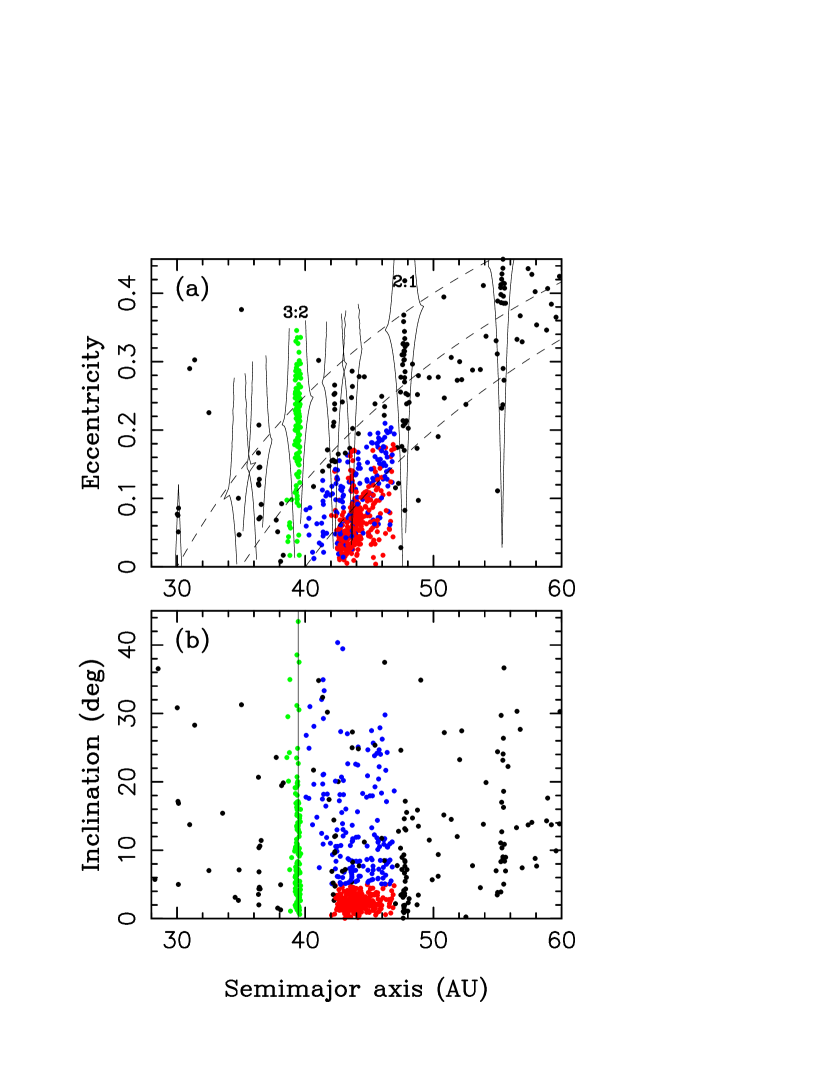
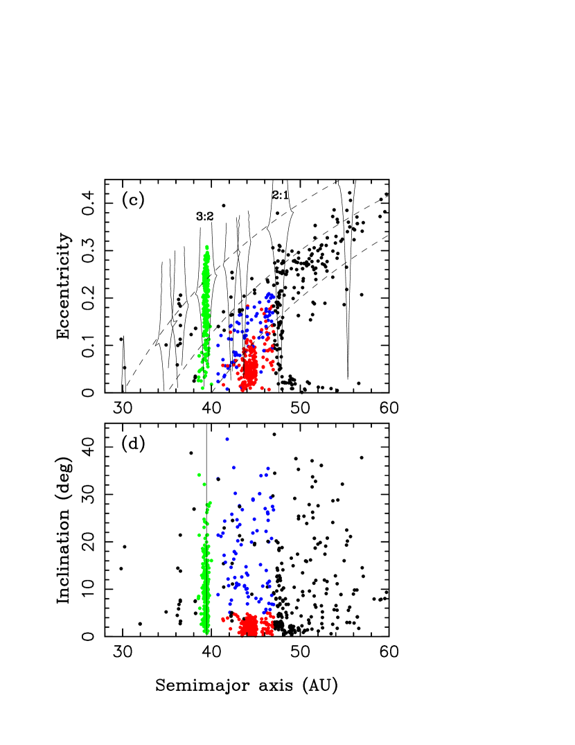
Figure 5 compares the OSSOS detections of KBOs (844 objects in total; some fall outside the plotted range) and tracked detections from the s30/100j model. To generate the model distribution in Fig. 5c,d, we use the raw orbital distribution from Fig. 3 and weights corresponding to the exponential disk profile with $r_{0}=24$ au and $\Delta r=2.5$ au. This profile gives the correct number of objects in different KBO populations as discussed in the previous section (Fig. 4a). To simulate the OSSOS detections, we adopt $D_{\rm break}=100$ km, $q_{\rm small}=2.1$ $q_{\rm big}=5$ and $p_{\rm V}=0.1$, and instruct the OSSOS simulator to detect and track 844 objects in total (the same as the total number of OSSOS detections).

The s30/100j model works well to reproduce the general orbital structure of the Kuiper belt. The model distribution shows populations of bodies in all main orbital resonances with Neptune, including Neptune Trojans in 1:1, Plutinos in 3:2 and Twotinos in 2:1. There are also tracked detections in the inner 4:3 resonance, the CKB resonances (e.g., 5:3, 7:4, 8:5), and the outer 5:2 resonance. An interesting difference between the OSSOS and model distributions is noted for the 2:1 and 5:2 resonances, where OSSOS detected important “core” populations (Fig. 5a,b; Volk et al. 2016, Chen et al. 2019). These populations are present in the raw results (Fig. 3) but are not sufficiently large to stand out in model detections (Fig. 5c,d). This issue is not related to Neptune’s jump because the same problem exists without a jump in the s30/100 simulation. The model with faster Neptune’s migration, s10/30j, performs better in this respect in that it shows the core populations in the 2:1 and 5:2 resonances, which are only factor of $\sim$2 below the number of objects actually detected by OSSOS.

The classical belt produced in the s30/100j model closely replicates the OSSOS CKB detections. There are HCs with a broad inclination distribution and CCs with low inclinations. The Kuiper belt kernel is notable in Fig. 5c,d and its orbital structure is very similar to that shown in Fig. 5a,b. We compare the orbital distributions of CCs in more detail below. There is a tail of low-eccentricity and low-inclination orbits beyond the 2:1 resonance which does not have a counterpart in the OSSOS detections. This may indicate that the radial profile of the original disk was steeper at 45-50 au than the one used here with $\Delta r=2.5$ au. For example, if we use $\Delta r=2$ au instead, the tail population near 50 au is reduced by a factor of $\sim$5, which would be more in line with OSSOS observations. This would also imply a much smaller CC population (Fig. 4a).

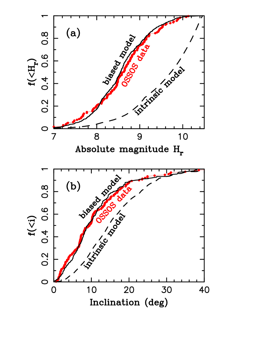
Figure 6 compares the orbital distributions for Plutinos. The intrinsic inclination distribution of Plutinos is very broad with the median $\simeq$15^∘. It matches, after being biased by the OSSOS simulator, the OSSOS detections. Here we used $\Delta r=2.5$ au. The s30/100j model with a truncated power-law profile and $c\simeq 1000$ works equally well. This means that the radial profile of the original planetesimal disk cannot be inferred from the orbital distribution of Plutinos alone. This information was lost during the implantation process. The s10/30j models with $\Delta r=2.5$ au or $c\simeq 1000$ produce similar results, but the biased model inclination distribution is slightly narrower than the observed one. A general correlation between the inclination distribution of KBOs and Neptune’s migration timescale was pointed out in Nesvorný (2015a; but see Volk & Malhotra 2019).

The OSSOS inclination distribution of HCs shows a potential break near 12^∘. Below this break the distribution is steeply raising such that approximately 60% of detected HCs have orbital inclinations below the break. The distribution is shallower above the break and extends to $i>30^{\circ}$. This feature has previously been noted in Nesvorný (2015a) and interpreted as a consequence of Neptune’s migration into an extended disk. Here we find that the high-$i$ part of the distribution is implanted from $r\lesssim 35$ au (implying more excitation) and the low-$i$ part started at $r\gtrsim 35$ au (implying less excitation). The inclination distribution of HCs may therefore help to constrain the radial profile of the original disk. The best results are obtained with $\Delta r>3$ au or $c<500$ for the s30/100j model creating some tension with our general preference for $\Delta r\simeq 2.5$ au or $c\simeq 1000$. The s10/30j models with $\Delta r\simeq 2.5$ au and $c\simeq 1000$ produce narrower inclination distributions. This may indicate that the actual migration timescale of Neptune was intermediate between the two timescales investigated here.

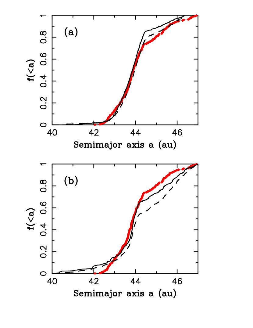
The s10/30j and s30/100j models produce the Kuiper belt kernel (Petit et al. 2011, Nesvorný 2015b). The kernel appears in the OSSOS observations as a strong concentration of low-$i$ KBOs near 44 au (Fig. 7; also see Fig. 5). The observed kernel has an outer edge at $\simeq$44.3 au, beyond which the number density of CCs drops by a factor of $\sim$5. The migration models with Neptune’s jump work well to reproduce these observations. The s10/30j model leads to a slightly stronger concentration of bodies below $\simeq$44.3 au (Fig. 7a), whereas the s30/100j model leads to a slightly weaker concentration (Fig. 7b). Again, this may indicate that the actual evolution of Neptune’s orbit was intermediate between our two models.

4.3 Colors

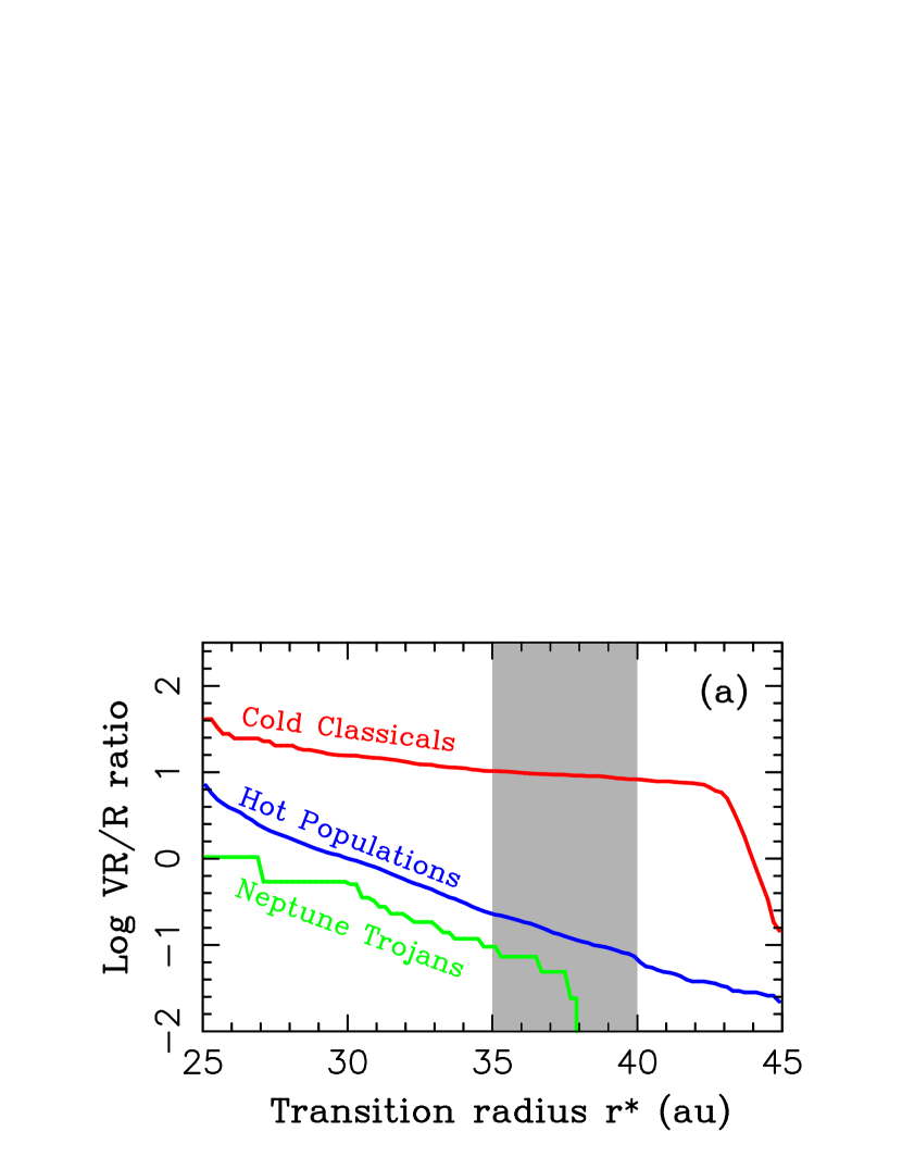
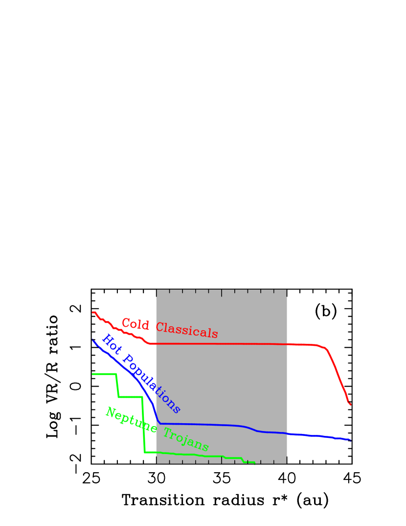
The intrinsic VR/R color ratios in different KBO populations are plotted for the s30/100j and s10/30j models in Figs. 8 and 9, respectively. In Fig. 8, we set $\Delta r=2.5$ au (panel a) and $c=1000$ (panel b) and plot the VR/R ratio as a function of the transition radius $r^{*}$. As expected, the VR/R ratios are inversely correlated with $r^{*}$ (i.e., lower VR/R values are obtained for larger transition radii). The profiles for the truncated power-law disks show a slope change near 30 au, which is a reflection of the surface density discontinuity in these models. The exponential disk models lead to a more continuous change of the VR/R ratio with the transition radius. In both cases, CCs show a nearly constant VR/R ratio for $30<r^{*}<43$ au and, for obvious reasons, a sudden drop just outside of 43 au. There is not much difference between the s10/30j and s30/100j models. We do not have sufficiently good statistics for NTs, because the number of bodies captured as Neptune’s co-orbitals is generally small. That is why the color ratios of NTs in Figs. 8 and 9 are choppy.

Comparing these results with the color constraints discussed in Sect. 3.3 we find that $35<r^{*}<40$ au for the exponential profile in Fig. 8a and $30<r^{*}<40$ au for the truncated power-law profile in Fig. 8b (s30/100j model). For example, using the exponential profile and $r^{*}=37$ au we find ${\rm VR/R}=10$ for CCs, ${\rm VR/R}=0.15$ for the hot populations, and ${\rm VR/R}=0.05$ for NTs. The truncated power-law profile and $r^{*}=35$ au lead to ${\rm VR/R}=10$ for CCs, ${\rm VR/R}=0.1$ for the hot populations, and ${\rm VR/R}=0.01$ for NTs.

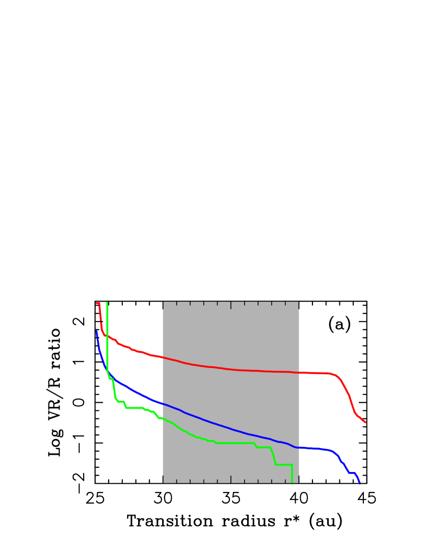
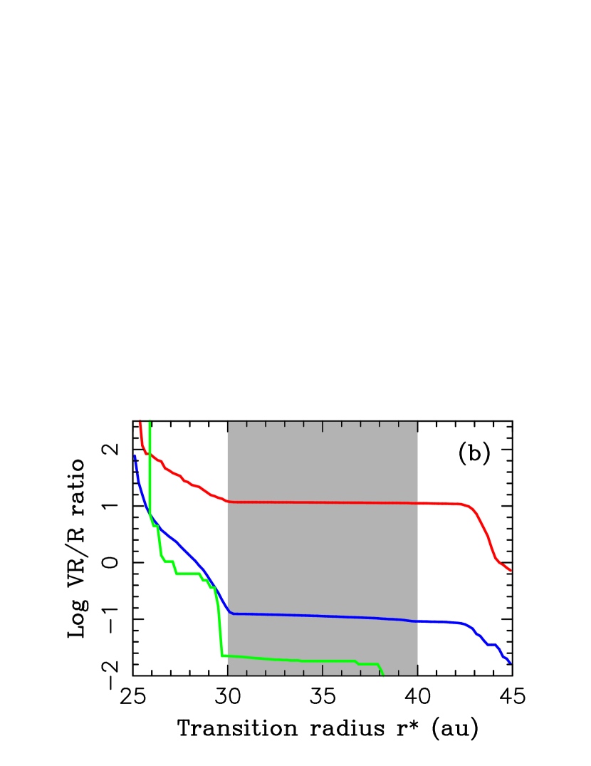
The general trends for the s10/30j model are similar (Fig. 9). Here we opted for using the exponential profile with $\Delta r=3$ au (panel a) and the truncated power-law profile with $c=300$ (panel b), because these parameters better match the color constraints. Specifically, for $\Delta r=3$ au and $r^{*}=35$ au, we obtain ${\rm VR/R}=7$ for CCs, ${\rm VR/R}=0.3$ for hot populations, and ${\rm VR/R}=0.06$ for NTs. If, $c=300$ and $r^{*}=35$ au instead, we get ${\rm VR/R}=10$ for CCs, ${\rm VR/R}=0.1$ for hot populations, and ${\rm VR/R}=0.02$ for NTs. All these cases therefore satisfactorily replicate the predominance of the VR colors among CCs, and the predominance of the R colors in other KBO populations. The color transition at $r^{*}<30$ au can be ruled out because the VR/R ratio would be generally too high. The color transition at $r^{*}>40$ au is not supported as well because the VR/R ratio would be generally too low. In summary, we find that $30<r^{*}<40$ au.

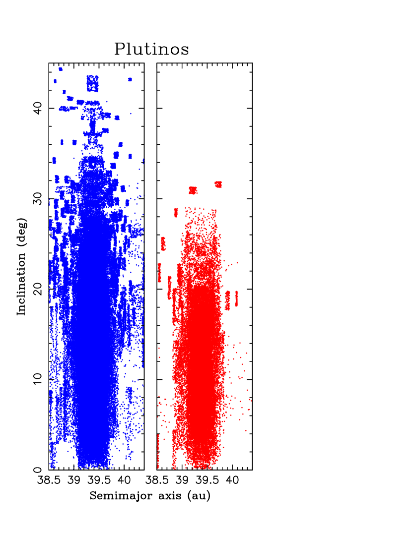
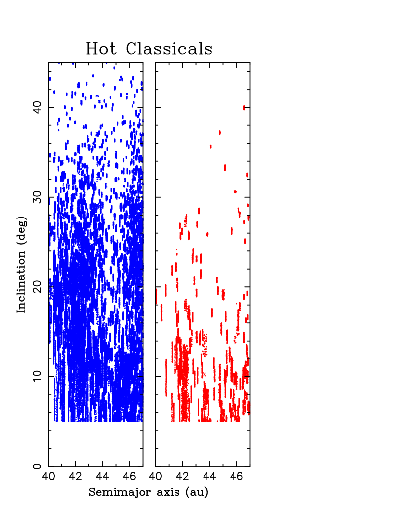
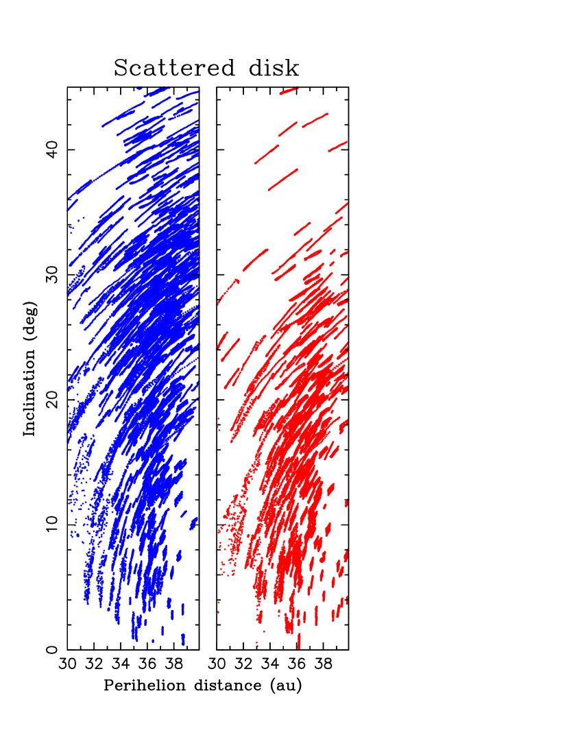
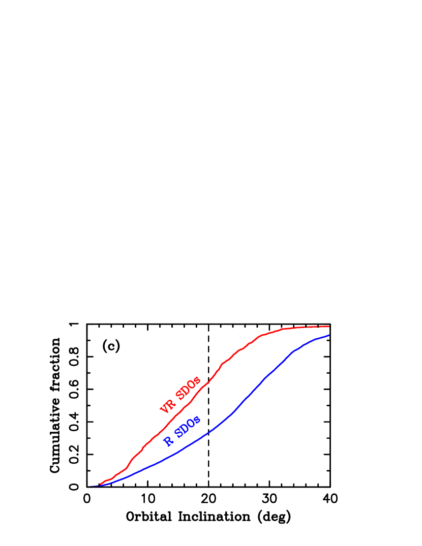
We now consider the correlation between colors and orbital inclinations (e.g., Marsset et al. 2019). For that, we use the s30/100j model with the exponential profile and $\Delta r=2.5$ au, and $r^{*}=37$ au (the results for other cases are similar, given that $30<r^{*}<40$ au). Bodies are separated into two color groups: R for bodies starting with $r<37$ au and VR for $r>37$ au. We plot the final orbits in Fig. 10. The figure shows that the R objects in each population –Plutinos, HCs and SDOs– are expected to have wider inclination distribution than the VR objects. The R objects starting in the inner disk have experienced, on average, stronger orbital perturbations from Neptune and ended with higher inclinations. This explains the observed correlation between colors and orbital inclinations, and provides strong support for the color hypothesis proposed here.

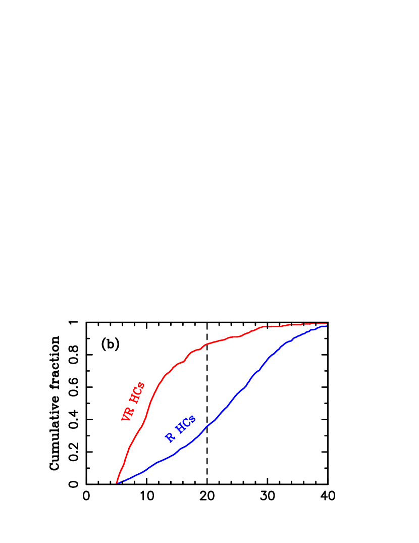
Figure 11 demonstrates this in more detail. Here we re-plot the model results from Fig. 10 as cumulative distributions. For example, $\simeq$95% of VR Plutinos are expected to have $i<20^{\circ}$, in a close correspondence to observations (Marsset et al. 2019). In contrast, $\simeq$30% of R Plutinos have $i>20^{\circ}$ (Fig. 11a). The R category dominates in the Plutino population, and, when biased, matches the OSSOS inclination distribution in Figure 6b. Both R and VR SDOs are expected to have broader inclination distributions than Plutinos (Fig. 11c). The inclination distribution of HCs is intermediate between Plutinos and SDOs. Interestingly, the HCs also show the biggest difference in the inclination distribution of R and VR bodies (Fig. 11b). This may be reflected in Fig. 3 of Marsset et al. (2019), where HCs characterized as VR by OSSOS cluster near $i=10^{\circ}$.

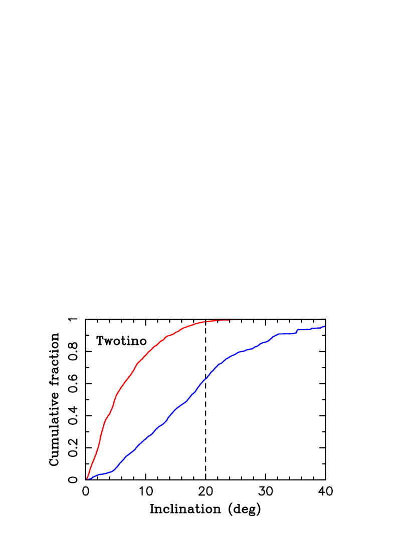
Finally, in Fig. 12, we show the inclination distributions of R and VR bodies in the 2:1 resonance (Twotinos). Overall, we find the intrinsic VR/R ratio to be $\simeq$0.4, whereas Sheppard (2012) reported 4 VR and 6 R Twotinos, suggesting observed VR/R $\sim 0.67$. These numbers indicate that Twotinos are a more equal mix of R and VR objects than other KBO populations (where, typically, one of the color groups dominates). In our model, this is caused by the 2:1 resonance migration over the $r<47$ au region and capture of low-inclination VR objects into the 2:1 resonance. The orbital inclinations are somewhat increased by capture but, as Fig. 12 shows, $\sim$80% of VR objects in the 2:1 resonance still have $i<10^{\circ}$. Our expectation is thus that the low-$i$ Twotinos should be predominantly VR, whereas Sheppard (2012) reported 2 R and 1 VR Twotinos with $i<5^{\circ}$. It would be useful to obtain colors for more low-$i$ Twotinos to understand whether they are indeed predominantly VR, as our model suggests. Another consequence of capture of low-$i$ objects into the 2:1 resonance is that the inclination distribution of Plutinos should be narrower than that of the 3:2 or 5:2 resonant populations. And this is indeed supported by observations (e.g., Chen et al. 2019).

5 Conclusions

The main findings of this work are:

1. The dynamical models with slow migration of Neptune reproduce the number of KBOs in different populations and their orbital distribution. The migration timescale is inferred to be intermediate between the s10/30j and s30/100j models (Table 1). The jumping Neptune model can explain the Kuiper belt kernel.

2. The different proportions of R and VR colors in different KBO populations can be explained if the R bodies formed at radial distances $r<r^{*}$ and the VR bodies at $r>r^{*}$, with $30<r^{*}<40$ au. The subsequent evolution mixed R and VR bodies into different populations.

3. The R to VR transition at $30<r^{*}<40$ au in the original planetesimal disk implies that the inclination distribution of R bodies should be broader than that of VR bodies, in a close correspondence to observations. This results provides support to the color hypothesis proposed here.

4. The exponential ($2.2<\Delta r<3.1$ au) and truncated power-law ($300<c<3000$) profiles of the original disk work equally well to reproduce various constraints. Additional work will be needed to distinguish between these possibilities.

The suggested transition from R to VR colors at 30-40 au can be a consequence of the sublimation-driven surface depletion in some organic molecules, such as NH₃ (Brown et al. 2011). In this case, the transition should have happened at the sublimation radius. An alternative possibility is that the R-to-VR transition traces different collisional histories of objects. Consider that the original planetesimal disk below 30 au was massive and could have suffered intense collisional grinding over its lifetime ($t_{\rm disk}<100$ Myr; Nesvorný 2018). This may have affected the surface properties of the planetesimals that emerged from $<$30 au (via impact related depletion and burial of volatiles). In contrast, the collisional activity beyond $\sim$30 au should have been relatively modest due to a lower disk surface density in this region. Note, however, that the magnitude distributions of R and VR objects in the dynamically hot populations are similar, at least in the range $7.5<H<9$ examined by Wong & Brown (2017), thus ruling out a substantial difference in the collisional history of 100-km-class KBOs.

Centaurs, presumed to have relatively recently evolved from the Kuiper belt, share the bimodality of colors and color-inclination correlation with hot KBOs (e.g., Wong & Brown 2017). Observations show that the VR colors of Centaurs disappear when objects reach $r\lesssim 10$ au (Jewitt 2015), probably due to the increased heating and removal/burial of the very red matter. This explains why Jupiter Trojans at 5 au cannot have VR colors. The primary reason behind the color similarity of Jupiter and Neptune Trojans (Jewitt 2018), however, is that both these populations formed at $r<r^{*}=30$-40 au and did not have the VR colors to start with.

6 Appendix A

The break in the size distributions of Jupiter Trojans and dynamically hot KBOs is often interpreted as a result of collisional grinding of planetesimals in the massive original disk before its dispersal by Neptune (e.g., Nesvorný & Vokrouhlický 2019; see also Pan & Sari 2005, Fraser 2009, Campo Bagatin & Benavidez 2012). The CC population, instead, given its low mass and distant orbits, has probably not experienced any intense period of collisional grinding. Its size distribution may thus reflect the initial mass function of planetesimals that was determined by early formation processes.

Here we use, inspired by existing simulations of the streaming instability (Youdin & Goodman 2005; see, e.g., Simon et al. 2017, Li et al. 2018), the cumulative size distribution

$$N(>\!\!D)=A\left({D\over D_{0}}\right)^{-p}\exp\left[-\left({D\over D_{0}}\right)^{q}\right]\,$$ (1)

where $A$, $p$, $q$ and $D_{0}$ are parameters. Here, $p$ is the cumulative power-law slope index of small bodies. The power law is exponentially tampered for bodies with $D\gtrsim D_{0}$. The albedo $p_{\rm V}=0.1$ is assumed to convert sizes to absolute magnitudes. By forward modeling the OSSOS observations of CCs, we find $A\simeq 1.3\times 10^{5}$, $p\simeq 0.6$, $q\simeq 1.2$ and $D_{0}\simeq 60$ km. The OSSOS calibration therefore implies $\sim$15,000 CCs (this is the number used in the main text) with $D>100$ km, which is a factor of several smaller population than the one reported by Petit et al. (2011). If $p_{\rm V}=0.2$ instead, we obtain $\sim$5,000 CCs with $D>100$ km. For comparison, CCs have mean $p_{\rm V}=0.13\pm 0.05$ (Müller et al. 2020) and Arrokoth –member of the CC population– has $p_{\rm V}=0.23$ (Spencer et al. 2020).

Our forward modeling of OSSOS detections also indicates that the current mass of CCs is $M_{\rm CC}\simeq 5\times 10^{-3}$ $M_{\rm Earth}$ for $\rho=1$ g cm^-3 bulk density and $p_{\rm V}=0.1$. If, instead, $p_{\rm V}=0.2$, then $M_{\rm CC}\simeq 2\times 10^{-3}$ $M_{\rm Earth}$. Adopting $\rho=0.5$ g cm^-3, as motivated by observations of Arrokoth and some CC binaries (Noll et al. 2020), would halve the total mass. In summary, we find $M_{\rm CC}=(3\pm 2)\times 10^{-3}$ $M_{\rm Earth}$, roughly $\sim$3-15 larger than the CC mass estimated in Fraser et al. (2014). Note that the size distribution is uncertain for $D<D_{0}$ where OSSOS did not detect a statistically large number of CCs.

In summary, we use the broken power-law distribution for bodies starting in the massive disk below 30 au and the exponentially tampered power-law distribution for bodies starting beyond 40 au. The transition radius, $r_{\rm trans}$ between these distributions is uncertain. We tested $30<r_{\rm trans}<40$ au and found that the orbital and color distribution of $D>100$ km bodies is relatively insensitive to the exact location of this transition. The $r_{\rm trans}$ parameter would mainly influence the population of very small KBOs, where the two distribution considered here differ the most, but that’s not the subject of this work. All the results reported in the main text were obtained with $r_{\rm trans}=40$ au. The results with no transition (i.e., for $r_{\rm trans}>50$ au) are similar.

migration	$a_{{\rm N},0}$	$\tau_{1}$	$\tau_{2}$	$\Delta a_{\rm N}$	$N_{\rm Pluto}$	$a_{\rm N}$	$P_{\rm N}/P_{\rm U}$
model	(au)	(Myr)	(Myr)	(au)		(au)
s10/30	24	10	30	0	2000	29.6	1.92
s10/30j	24	10	30	0.4	2000	30.1	1.95
s30/100	24	30	100	0	4000	29.7	1.95
s30/100j	24	30	100	0.5	4000	29.9	1.94

Table 1: A two stage migration of Neptune was adopted from Nesvorný & Vokrouhlický (2016): $\tau_{1}$ and $\tau_{2}$ define the $e$-folding exponential migration timescales during these stages, $a_{\rm N,0}$ and $a_{\rm N}$ denotes Neptune’s initial and final semimajor axes, $\Delta a_{\rm N}$ is the jump applied to Neptune’s semimajor axis at the transition between stages 1 and 2, $N_{\rm Pluto}$ is the assumed initial number of Pluto-mass objects in the massive disk below 30 au (Nesvorný & Vokrouhlický 2016). The last columns show the final semimajor axis of Neptune and the orbital period ratio of Uranus and Neptune. For reference, $a_{\rm N}=30.11$ au and $P_{\rm N}/P_{\rm U}=1.96$ in the current Solar System. The leading letter “s” in the simulation names indicates that both these migrations are considered to be slow (Nesvorný 2015a), the trailing letter “j” indicates whether a jump has been applied to Neptune at the transition between Stages 1 and 2.

Figure 1: The orbit histories of the giant planets obtained in a self-consistent migration simulation with a planetesimal disk between 24 and 60 au (total disk mass $M_{\rm disk}=20$ $M_{\rm Earth}$). The initial surface density of planetesimals was assumed to follow a radial profile with exponentially decreasing surface density from 24 to 60 au with one e-fold $\Delta r=2.5$ au (no disk truncation at 30 au). The plot shows the semimajor axes (solid lines) and perihelion/aphelion distances (thin dashed lines) of each planet’s orbit. The fifth planet (labeled Ice 3) was ejected from the Solar System by Jupiter during the instability (integration time $t=11.7$ Myr). The solid black lines are Neptune’s exponential migration fits with $\tau_{1}=12$ Myr for $t<11.7$ Myr (Stage 1; labeled S1) and $\tau_{2}=27$ Myr for $t>11.7$ Myr (Stage 2). The final orbits of the planets are a good match to those in the present Solar System.

Figure 2: Three planetesimal disk profiles used in this work: (a) truncated power law, (b) exponential, and (c) power-law inner disk and exponential outer disk. The surface density is arbitrarily normalized here to $\Sigma=1$ at 24 au.

Figure 3: The raw orbital distribution of KBOs obtained in the s30/100j model. The final orbits of planetesimals starting with $a<35$ au ($a>35$ au) are plotted as blue (red) dots in panels a and b (c and d). The dashed lines show the location of the 3:2 resonance with Neptune ($a=39.45$ au in a and c), perihelion distance $q=36$ au (a and c), and inclinations $i=5^{\circ}$ and 20^∘ (panels b and d).

Figure 4: The population estimates from the s30/100j model for different initial profiles of the original planetesimal disk. Different lines correspond to the main CKB (black), HCs (blue), CCs (red), Plutinos (green) and Neptune Trojans (yellow). The top panel is the exponential profile starting at $r_{0}=24$ au. The bottom panel is the truncated power-law profile with a surface density drop at 30 au. The shaded areas highlight the plausible range of parameters. The exponential profiles with $\Delta r<2.2$ au can be ruled out because the population of CCs predicted in such models is too small ($<$7,000 $D>100$ km bodies; most CCs would be deposited onto their present orbits from $r<30$ au if $\Delta r<1.5$ au). Similarly, the exponential models with $\Delta r>3.1$ au can be ruled because the predicted number of CCs is excessive ($>$50,000 $D>100$ km bodies for $\Delta r>3.1$ au). Similar arguments based on the CC population can be used to rule out $c<300$ and $c>3000$ for the case shown in panel (b).

Figure 5: The OSSOS KBOs (left panels) and tracked detections from the s30/100j model with $\Delta r=2.5$ au (right panels). In both cases, the plots show the barycentric orbital elements referred to the center of mass of the Solar System. For ease of comparison different populations are highlighted by different colors: Plutinos (green dots), HCs (blue dots) and CCs (red dots). The orbital elements of all other KBOs are shown as black dots.

Figure 6: A comparison between the biased model (solid black line) and OSSOS observations (red dots) of Plutinos in the 3:2 resonance with Neptune. Following the method described in Section 3 we simulate resonant capture of Plutinos from the original planetesimal disk. The OSSOS simulator was then applied to the present-day intrinsic model distribution (dashed lines). The large difference between the intrinsic and biased distributions illustrates the extreme biases of KBO observations and the importance of the OSSOS simulator. These results were obtained with an exponential disk profile ($r_{0}=24$ au, $\Delta r=2.5$ au, $M_{\rm disk}=20$ $M_{\rm Earth}$). See Fig. 1 for Neptune’s migration in this case. The (biased model) absolute magnitude (panel a) and orbital inclination (panel b) distributions match OSSOS observations. The results for orbital eccentricities and libration amplitudes, not shown here, are equally good.

Figure 7: A comparison between the biased models (solid black lines) and OSSOS observations (red dots) of CCs ($i<5^{\circ}$). The intrinsic semimajor axis distributions obtained in our models are shown by dashed lines. Panel (a) shows the result for the s10/30j model and panel (b) shows the result for the s30/100j model. The Kuiper belt kernel is represented by a steeply raising semimajor axis distribution toward a break near 44.3 au.

Figure 8: The intrinsic VR/R ratio in the s30/100j model for different initial profiles of the original planetesimal disk: the (a) exponential profile with $\Delta r=2.5$ au, and (b) truncated power-law profile with $c=1000$. Different lines correspond to CCs (red), hot populations (blue) and Neptune Trojans (green). The shaded area approximately highlights the possible range of VR/R transition radii in the original disk.

Figure 9: The intrinsic VR/R ratio in the s10/30j model for different initial profiles of the original planetesimal disk: the (a) the exponential profile with $\Delta r=3$ au, and (b) truncated power-law profile with $c=300$. The different lines correspond to CCs (red), hot populations (blue) and Neptune Trojans (green). The shaded area approximately highlights the possible range of VR/R transition radii in the original disk.

Figure 10: The inclination distribution of R (blue dots) and VR (red dots) bodies obtained in the s30/100j model with $\Delta r=2.5$ au and $r^{*}=37$ au. We show the distributions for Plutinos (left panels), HCs (middle panels) and SDOs (right panels). For each individual object, we plot 100 orbits from the 10 Myr integration starting at $t=4.5$ Gyr (see Section 3.3). Only orbits with $i>5^{\circ}$ are plotted in the middle plots to avoid confusion with CCs. In all three cases, the inclination distribution of R objects is broader than the inclination distribution of the VR objects. Compare to Fig. 3 in Marsset et al. (2019).

Figure 11: The proposed color hypothesis implies that the occurrence of R and VR objects in the hot populations should correlate with orbital inclination. Here we take the model results from Fig. 10 and plot them as cumulative distributions. Panels (a), (b) and (c) show Plutinos, HCs and SDOs, respectively. In all cases, the R bodies have a significantly broader inclination distribution than the VR bodies, as observed.

Figure 12: The intrinsic inclination distributions of R (blue line) and VR (red line) Twotinos in the 2:1 resonance with Neptune obtained in the s30/100j model ($\Delta r=2.5$ au and $r^{*}=37$ au). About 80% of VR Twotinos are expected to have $i<10^{\circ}$.

References

- Bannister et al. (2018) Bannister, M. T., Gladman, B. J., Kavelaars, J. J., et al. 2018, ApJS, 236, 1 8
- Barucci et al. (2005) Barucci, M. A., Belskaya, I. N., Fulchignoni, M., Birlan, M. 2005, AJ, 130, 1291
- Batygin et al. (2011) Batygin, K., Brown, M. E., & Fraser, W. C. 2011, EPSC-DPS Joint Meeting 2011, 1154
- Brown (2001) Brown, M. E. 2001, AJ, 121, 2804
- Brown et al. (2011) Brown, M. E., Schaller, E. L., & Fraser, W. C. 2011, ApJ, 739, L60
- Chen et al. (2019) Chen, Y.-T., Gladman, B., Volk, K., et al. 2019, AJ, 158, 214
- Deienno et al. (2017) Deienno, R., Morbidelli, A., Gomes, R. S., & Nesvorný, D. 2017, AJ, 153, 153
- Emery et al. (2015) Emery, J. P., Marzari, F., Morbidelli, A., French, L. M., & Grav, T. 2015, Asteroids IV, 203
- Fraser and Brown (2012) Fraser, W. C., Brown, M. E. 2012, ApJ, 749, 33
- Fraser et al. (2014) Fraser, W. C., Brown, M. E., Morbidelli, A., Parker, A., & Batygin, K. 2014, ApJ, 782, 100
- Fraser et al. (2017) Fraser, W. C., Bannister, M. T., Pike, R. E., et al. 2017, Nature Astronomy, 1, 0088
- Gladman et al. (2008) Gladman, B., Marsden, B. G., & Vanlaerhoven, C. 2008, The Solar System Beyond Neptune, 43
- Gomes, & Nesvorný (2016) Gomes, R., & Nesvorný, D. 2016, A&A, 592, A146
- Gomes et al. (2004) Gomes, R. S., Morbidelli, A., & Levison, H. F. 2004, Icarus, 170, 492
- Graykowski, & Jewitt (2018) Graykowski, A., & Jewitt, D. 2018, AJ, 155, 184
- Hahn & Malhotra (2005) Hahn, J. M., & Malhotra, R. 2005, AJ, 130, 2392
- Hainaut and Delsanti (2002) Hainaut, O. R., Delsanti, A. C. 2002, A&A, 389, 641
- Hamilton, & Ward (2004) Hamilton, D. P., & Ward, W. R. 2004, AJ, 128, 2510
- Jewitt (2018) Jewitt, D. 2018, AJ, 155, 56
- Jewitt (2015) Jewitt, D. 2015, AJ, 150, 201
- Jewitt and Luu (1998) Jewitt, D., Luu, J. 1998, AJ, 115, 1667
- Jewitt and Luu (2001) Jewitt, D. C., Luu, J. X. 2001, AJ, 122, 2099
- Lawler et al. (2018) Lawler, S. M., Kavelaars, J. J., Alexandersen, M., et al. 2018a, Frontiers in Astronomy and Space Sciences, 5, 14
- Lawler et al. (2018) Lawler, S. M., Shankman, C., Kavelaars, J. J., et al. 2018b, AJ, 155, 197
- Levison, & Duncan (1994) Levison, H. F., & Duncan, M. J. 1994, Icarus, 108, 18
- Li et al. (2018) Li, R., Youdin, A. N., & Simon, J. B. 2018, ApJ, 862, 14
- Luu and Jewitt (1996) Luu, J., Jewitt, D. 1996, AJ, 112, 2310
- Luu and Jewitt (1998) Luu, J. X., Jewitt, D. C. 1998, ApJ, 494, L117
- Marsset et al. (2019) Marsset, M., Fraser, W. C., Pike, R. E., et al. 2019, AJ, 157, 94
- Morbidelli et al. (2005) Morbidelli, A., Levison, H. F., Tsiganis, K., & Gomes, R. 2005, Nature, 435, 462
- Müller et al. (2020) Müller, T., Lellouch, E., & Fornasier, S. 2020, The Trans-neptunian Solar System, 153
- Nesvorný (2015) Nesvorný, D. 2015a, AJ, 150, 73
- Nesvorný (2015) Nesvorný, D. 2015b, AJ, 150, 68
- Nesvorný (2018) Nesvorný, D. 2018, ARA&A, 56, 137
- Nesvorný, & Vokrouhlický (2009) Nesvorný, D., & Vokrouhlický, D. 2009, AJ, 137, 5003
- Nesvorný & Morbidelli (2012) Nesvorný, D., & Morbidelli, A. 2012 (NM12), AJ, 144, 117
- Nesvorný & Vokrouhlický (2016) Nesvorný, D., & Vokrouhlický, D. 2016, ApJ, 825, 94
- Nesvorný, & Vokrouhlický (2019) Nesvorný, D., & Vokrouhlický, D. 2019, Icarus, 331, 49
- Nesvorný et al. (2013) Nesvorný, D., Vokrouhlický, D., & Morbidelli, A. 2013, ApJ, 768, 45
- Nesvorný et al. (2019) Nesvorný, D., Vokrouhlický, D., Stern, A. S., et al. 2019a, AJ, 158, 132
- Noll et al. (2020) Noll, K., Grundy, W. M., Nesvorný, D., et al. 2020, The Trans-neptunian Solar System, 201
- Peixinho et al. (2003) Peixinho, N., Doressoundiram, A., Delsanti, A. et al. 2003, A&A, 410, L29
- Peixinho et al. (2008) Peixinho, N., Lacerda, P., & Jewitt, D. 2008, AJ, 136, 1837
- Peixinho et al. (2012) Peixinho, N., Delsanti, A., Guilbert-Lepoutre, A., et al. 2012, A&A, 546, A86
- Peixinho et al. (2015) Peixinho, N., Delsanti, A., Doressoundiram, A. 2015. A&A, 577, A35
- Parker et al. (2013) Parker, A. H., Buie, M. W., Osip, D. J., et al. 2013, AJ, 145, 96
- Parker (2015) Parker, A. H. 2015, Icarus, 247, 112
- Petit et al. (2011) Petit, J.-M., Kavelaars, J. J., Gladman, B. J., et al. 2011, AJ, 142, 131
- Pike et al. (2017) Pike, R. E., Fraser, W. C., Schwamb, M. E., et al. 2017, AJ, 154, 101
- Pirani et al. (2019) Pirani, S., Johansen, A., & Mustill, A. J. 2019, A&A, 631, A89
- Schwamb et al. (2019) Schwamb, M. E., Fraser, W. C., Bannister, M. T., et al. 2019, ApJS, 243, 12
- Sheppard (2012) Sheppard, S. S. 2012, AJ, 144, 169
- Sheppard, & Trujillo (2006) Sheppard, S. S., & Trujillo, C. A. 2006, Science, 313, 511
- Simon et al. (2017) Simon, J. B., Armitage, P. J., Youdin, A. N., et al. 2017, ApJ, 847, L12
- Spencer et al. (2020) Spencer, J. R., Stern, S. A., Moore, J. M., et al. 2020, Science, 367, aay3999
- Tegler and Romanishin (1998) Tegler, S. C., Romanishin, W. 1998, Nature 392, 49
- Tegler and Romanishin (2000) Tegler, S. C., Romanishin, W. 2000, Nature, 407, 979
- Tegler et al. (2003) Tegler, S. C., Romanishin, W., Consolmagno, G. J. 2003, ApJ599, L49
- Tegler et al. (2016) Tegler, S. C., Romanishin, W., Consolmagno, G. J. 2016, AJ, 152, 210
- Trujillo and Brown (2002) Trujillo, C. A., Brown, M. E. 2002, ApJ, 566, L125
- Vokrouhlický, & Nesvorný (2015) Vokrouhlický, D., & Nesvorný, D. 2015, ApJ, 806, 143
- Volk, & Malhotra (2019) Volk, K., & Malhotra, R. 2019, AJ, 158, 64
- Volk et al. (2016) Volk, K., Murray-Clay, R., Gladman, B., et al. 2016, AJ, 152, 23
- Ward, & Hamilton (2004) Ward, W. R., & Hamilton, D. P. 2004, AJ, 128, 2501
- Wong & Brown (2015) Wong, I., & Brown, M. E. 2015, AJ, 150, 174
- Wong, & Brown (2016) Wong, I., & Brown, M. E. 2016, AJ, 152, 90
- Wong, & Brown (2017) Wong, I., & Brown, M. E. 2017, AJ, 153, 145
- Yoshida, & Terai (2017) Yoshida, F., & Terai, T. 2017, AJ, 154, 71
- Youdin, & Goodman (2005) Youdin, A. N., & Goodman, J. 2005, ApJ, 620, 459