Studying The Effect of MIL Pooling Filters
on MIL Tasks

Abstract

There are different multiple instance learning (MIL) pooling filters used in MIL models. In this paper, we study the effect of different MIL pooling filters on the performance of MIL models in real world MIL tasks. We designed a neural network based MIL framework with 5 different MIL pooling filters: ‘max’, ‘mean’, ‘attention’, ‘distribution’ and ‘distribution with attention’. We also formulated 5 different MIL tasks on a real world lymph node metastases dataset. We found that the performance of our framework in a task is different for different filters. We also observed that the performances of the five pooling filters are also different from task to task. Hence, the selection of a correct MIL pooling filter for each MIL task is crucial for better performance. Furthermore, we noticed that models with ‘distribution’ and ‘distribution with attention’ pooling filters consistently perform well in almost all of the tasks. We attribute this phenomena to the amount of information captured by ‘distribution’ based pooling filters. While point estimate based pooling filters, like ‘max’ and ‘mean’, produce point estimates of distributions, ‘distribution’ based pooling filters capture the full information in distributions. Lastly, we compared the performance of our neural network model with ‘distribution’ pooling filter with the performance of the best MIL methods in the literature on classical MIL datasets and our model outperformed the others.

1 Introduction

Multiple instance learning (MIL) is a machine learning paradigm which learns the mapping between bags of instances and bag labels. In real life, MIL models are handy for tasks where data is in the form of bags of instances and only bag labels are provided. For example, medical image processing tasks are typical MIL tasks since an image can be treated as a bag of pixels (instances) and there usually exists only an image (bag) label without providing the particular region-of-interest [1].

Although positive vs negative bag classification [2, 3] is the most commonly used version of MIL tasks, there are other MIL tasks in the literature as well, like unique class count prediction [4], multi-class classification [5], multi-task classification [6] or regression [7]. In order to solve these MIL tasks, different methods have been developed. While some methods first classify instances inside bags and then pool the instances’ scores by using an MIL pooling filter [2, 3, 8, 9], others first extract features of instances inside bags, obtain bag level representations by using an MIL pooling filter and finally classify the bags [10, 11, 4]. The common component in the two approaches is the MIL pooling filter. There are different MIL pooling filters, such as ‘max’ pooling [10, 12, 5], ‘mean’ pooling [10, 13] or ‘log-sum-exp’ pooling [14]. However, their performance on different MIL tasks may be different. Indeed, it was, for example, shown that ‘linear softmax’ pooling [15] performed best among five different MIL pooling filters (‘max’, ‘mean’, ‘linear softmax’, ‘exponential softmax’ and ‘attention’) on MIL task of sound event detection [13]. Hence, the choice of MIL pooling filter based on MIL task is crucial.

In this paper, our objective is to investigate the effect of different MIL pooling filters on the performance of an MIL model in a real world MIL task. With this objective, we designed neural network based MIL models with five different MIL pooling filters. We also formulated five different MIL tasks on a real world lymph node metastases dataset in [4] and applied our models on these tasks.

The lymph node metastases dataset consists of images cropped from histopathology slides of lymph node sections [16] and has corresponding ground truth metastases segmentation masks. There are three types of images in this dataset: fully normal - all cells are normal, fully metastases - all cells are metastases and boundary - mixture of normal and metastases cells. We formulated five different MIL tasks on this dataset: (i) positive vs negative bag classification, (ii) unique class count prediction, (iii) multi-class classification, (iv) multi-task classification and (v) regression. In positive vs negative bag classification, our task is to predict whether an image contains metastases cells or not. Precisely, a positive bag is either a fully metastases image or a boundary image. A negative bag is a fully normal image. In regression, our task is to predict the percentage of metastases pixels inside the image. For the other MIL tasks, they are defined in Sec. 4.1. For each MIL task, we trained five different models with five different MIL pooling filters, namely (i) ‘max’ pooling, (ii) ‘mean’ pooling, (iii) ‘attention’ pooling [11], (iv) ‘distribution’ pooling [4] and (v) ‘distribution with attention’ pooling. We developed ‘distribution with attention’ pooling by incorporating an attention mechanism similar to [11] into ‘distribution’ pooling. Furthermore, we examined the power of exploiting the full information in distributions by using ‘distribution’ pooling over using point estimates obtained by ‘mean’ and ‘max’ pooling in an MIL task of bag of metal balls classification. Lastly, although ‘distribution’ pooling was used in a novel MIL task of unique class count prediction in [4], it has never been tested on classical MIL datasets. Therefore, we tested its performance on classical MIL datasets and it outperformed state-of-the-art MIL methods.

Hence, there are four main contributions of this paper:

1. By examining the performance of MIL models with 5 different pooling filters on 5 different tasks formulated on the lymph node metastases dataset, we showed that different MIL pooling filters have different performances on different MIL tasks.

2. We showed that ‘distribution’ based pooling filters have better overall performance than point estimate based pooling filters, such as ‘mean’ and ‘max’ pooling since they capture full information in distributions rather than point estimates.

3. We showed that our model with ‘distribution’ pooling filter outperformed state-of-the-art MIL methods on classical MIL datasets.

4. We developed a new MIL pooling filter, ‘distribution with attention’ pooling filter, by incorporating an attention mechanism into ‘distribution’ pooling filter.

For the rest of the paper, Sec. 2 introduces our MIL framework; Sec. 3 gives a brief literature review; Sec. 4 defines the experiments and presents the results and Sec. 5 concludes the paper.

2 Multiple Instance Learning Framework

In MIL paradigm, the objective is to predict a bag label $Y$ for a given bag of instances $X=\{x_{i}|x_{i}\in\mathcal{I},i=1,2,\cdots,N\}$ where $\mathcal{I}$ is the instance space and $N$ is the number of instances inside the bag. Each instance $x_{i}\in X$ is endowed with an underlying label $y_{i}\in\mathcal{L}$, where $\mathcal{L}$ is the instance label space; however, these labels are inaccessible during training. The relation between bag label $Y$ and instance labels ${\{y_{i}|y_{i}\in\mathcal{L},i=1,2,\cdots,N\}}$ is imposed by the definition of MIL task. Note that although the number of instances in each bag can be different in real world, it is treated as constant in here for clarity of notation, yet all the properties stated in here are valid for bags with variable number of instances as well.

Figure 1: Block diagram of MIL framework. The feature extractor module $\theta_{\mbox{\tiny feature}}$ extracts a feature vector $\bm{f}_{x_{i}}\in\mathcal{F}$, $\forall x_{i}\in X$. Then, the MIL pooling filter module $\operatorname*{\theta_{\mbox{\tiny filter}}}$ aggregates the extracted feature vectors and obtains a bag level representation $\bm{h}_{X}\in\mathcal{H}$. Lastly, the bag level representation transformation module $\theta_{\mbox{\tiny transform}}$ transforms bag level representation into predicted bag label $\hat{Y}\in\mathcal{Y}$.

Let $\mathcal{D}$ be an MIL dataset such that $\mathcal{D}=\{(X,Y)\ |\ X\in\mathcal{X}\ and\ Y\in\mathcal{Y}\}$, where $\mathcal{X}=\mathcal{I}^{N}$ is the bag space and $\mathcal{Y}$ is the bag label space. Given any pair $(X,Y)\in\mathcal{D}$, our objective is to predict bag label $Y$ for a given bag of instances $X=\{x_{i}|x_{i}\in\mathcal{I},i=1,2,\cdots,N\}$. Let $\hat{Y}$ be predicted bag label of $X$. We obtain $\hat{Y}$ by using a three stage framework, block diagram of which is given in Figure 1. The first stage is a feature extractor module $\theta_{\mbox{\tiny feature}}:\mathcal{I}\rightarrow\mathcal{F}$, where $\mathcal{F}$ is the feature space. The feature extractor module takes an instance as input and outputs a feature vector: $\bm{f}_{x_{i}}=\theta_{\mbox{\tiny feature}}(x_{i})\in\mathcal{F}$ for each instance $x_{i}\in X$. The second stage is an MIL pooling filter module $\operatorname*{\theta_{\mbox{\tiny filter}}}:\mathcal{F}^{N}\rightarrow\mathcal{H}$, where $\mathcal{H}$ is the bag level representation space. The MIL pooling filter module takes the set of extracted feature vectors $\bm{F}_{X}=\{\bm{f}_{x_{i}}|x_{i}\in X,i=1,\cdots N\}$ and aggregates them to obtain a bag level representation: $\bm{h}_{X}=\operatorname*{\theta_{\mbox{\tiny filter}}}(\bm{F}_{X})\in\mathcal{H}$. For example, ‘max’ pooling gets maximum value of each feature over the feature vectors of all instances or ‘mean’ pooling calculates the mean of each feature over the feature vectors of all instances. In this paper, we analyze the performance of 5 different MIL pooling filters (see Sec. 2.2) on 5 different MIL tasks. The last stage is a bag level representation transformation module $\theta_{\mbox{\tiny transform}}:\mathcal{H}\rightarrow\mathcal{Y}$. The bag level representation transformation module transforms bag level representation into predicted bag label: $\hat{Y}=\theta_{\mbox{\tiny transform}}(\bm{h}_{X})$.

2.1 Modeling MIL with Neural Networks

We use neural networks to implement the feature extractor module $\theta_{\mbox{\tiny feature}}$ and the bag level representation transformation module $\theta_{\mbox{\tiny transform}}$ so that we can fully parameterize the learning process. For MIL pooling filter module $\operatorname*{\theta_{\mbox{\tiny filter}}}$, we use different kinds of filters, some of which also incorporate trainable components parameterized by neural networks. This system of neural network modules are end-to-end trainable.

Formally, given a bag of instances $X=\{x_{i}|x_{i}\in\mathcal{I},i=1,2,\cdots,N\}$, for each $x_{i}\in X$, $\theta_{\mbox{\tiny feature}}$ module extracts $J$ features $[f_{x_{i}}^{j}|f_{x_{i}}^{j}\in\mathbb{R},j=1,2,\cdots,J]=\bm{f}_{x_{i}}\in\mathcal{F}$ where $\mathcal{F}=\mathbb{R}^{J}$. After obtaining the set of extracted feature vectors $\bm{F}_{X}=\{\bm{f}_{x_{i}}|x_{i}\in X,i=1,\cdots N\}$, $\operatorname*{\theta_{\mbox{\tiny filter}}}$ module obtains bag level representation $\bm{h}_{X}\in\mathcal{H}$ where $\mathcal{H}$ depends on $\operatorname*{\theta_{\mbox{\tiny filter}}}$. Finally, $\theta_{\mbox{\tiny transform}}$ transforms $\bm{h}_{X}$ into predicted bag label $\hat{Y}\in\mathcal{Y}$. This notation is also used while defining MIL pooling filters in Sec. 2.2.

2.2 MIL pooling filters

An MIL pooling filter is used to aggregate instance level representations (extracted feature vectors of instances inside a bag) in order to obtain a bag level representation. As a key component of an MIL model, the MIL pooling filter provides the MIL model with two essential properties of MIL paradigm necessitated by set definition (note that a bag is nothing but a set). First, output of the model must be permutation-invariant, i.e. the model must produce the same output regardless of ordering of elements in the set. Second, the model must accept sets with variable sizes as input. These two properties are incorporated in our neural network model with the proper choice of the MIL pooling filters.

Max pooling:

‘Max’ pooling filter obtains bag level representation by capturing maximum activation of each feature across the extracted features of instances inside a bag. Bag level representation $\bm{h}_{X}=[h^{j}_{X}\ |\ h^{j}_{X}\in\mathbb{R},j=1,2,\cdots,J]\in\mathcal{H}$ where $\mathcal{H}=\mathbb{R}^{J}$ and $h^{j}_{X}=\max_{i=1}^{N}f_{x_{i}}^{j}\ \forall_{j=1,2,\cdots,J}$.

Mean pooling:

‘Mean’ pooling filter calculates bag level representation by getting the mean across the extracted features of all the instances inside a bag. Bag level representation $\bm{h}_{X}=[h^{j}_{X}\ |\ h^{j}_{X}\in\mathbb{R},j=1,2,\cdots,J]\in\mathcal{H}$ where $\mathcal{H}=\mathbb{R}^{J}$ and $h^{j}_{X}=\frac{1}{N}\sum_{i=1}^{N}f_{x_{i}}^{j}\ \forall_{j=1,2,\cdots,J}$.

Attention pooling:

‘Attention’ pooling was introduced in [11]. In this method, bag level representation is obtained by weighted sum of extracted features of instances in a bag. Bag level representation $\bm{h}_{X}=[h^{j}_{X}\ |\ h^{j}_{X}\in\mathbb{R},j=1,2,\cdots,J]\in\mathcal{H}$ where $\mathcal{H}=\mathbb{R}^{J}$ and $h^{j}_{X}=\sum_{i=1}^{N}w_{i}f_{x_{i}}^{j}\ \forall_{j=1,2,\cdots,J}$. Note that each instance has an attention based weight obtained from a neural network module $\mathcal{W}$ and instances’ weights sum up to 1, as shown in Eq. 1.

$$w_{i}=\frac{\exp\{\mathcal{W}(\bm{f}_{x_{i}})\}}{\sum_{t=1}^{N}\exp\{\mathcal{W}(\bm{f}_{x_{t}})\}}\ \forall_{i=1,2,\cdots,N}$$ (1)

Distribution pooling:

‘Distribution’ pooling as MIL pooling filter was introduced in [4]. Firstly, marginal distribution of each extracted feature is estimated. Let $\tilde{p}^{j}_{X}(v)$ be the estimated marginal distribution of $j^{th}$ extracted feature. We obtain $\tilde{p}^{j}_{X}(v)$ by using kernel density estimation [17], which employs a Gaussian kernel with standard deviation $\sigma$, as shown in the Eq. 2. Then, the estimated marginal distribution is sampled with $M$ bins as shown in Eq. 3 to obtain corresponding $h^{j}_{X}\in\mathbb{R}^{M}$. Hence, bag level representation $\bm{h}_{X}=[h^{j}_{X}\ |\ h^{j}_{X}\in\mathbb{R}^{M},j=1,2,\cdots,J]\in\mathcal{H}$ where $\mathcal{H}=\mathbb{R}^{MJ}$.

$$\tilde{p}^{j}_{X}(v)=\frac{1}{N}\sum_{i=1}^{N}\frac{1}{\sqrt{2\pi{\sigma}^{2}}}e^{-\frac{1}{2{\sigma}^{2}}\left(v-f_{x_{i}}^{j}\right)^{2}}\ \forall_{j=1,2,\cdots,J}$$ (2)

$$h^{j}_{X}=\left[\tilde{p}^{j}_{X}(v=v_{b})\ |\ v_{b}=\frac{b}{M-1}\text{ and }b=0,1,\cdots,M-1\right]\ \forall_{j=1,2,\cdots,J}\text{ where }h^{j}_{X}\in\mathbb{R}^{M}$$ (3)

Theoretically, full information in the extracted features can be captured by estimating the joint distribution; however, it is computationally intractable. Therefore, marginal distributions of extracted features are estimated to capture as much information as possible in ‘distribution’ pooling. ‘Distribution’ pooling has a notable advantage that it enables $\theta_{\mbox{\tiny transform}}$ module to fully utilize the information in shape of the distribution rather than looking at point estimates of it obtained by ‘mean’ and ‘max’ pooling filters. In principle, with a perfect $\operatorname*{\theta_{\mbox{\tiny filter}}}$ and $\theta_{\mbox{\tiny transform}}$ modules, the point estimates obtained by ‘mean’ and ‘max’ pooling filters can be fully recovered from the estimated marginal distributions obtained by ‘distribution’ pooling. Hence, the information contained in the bag level representations derived by ‘max’ and ‘mean’ pooling filters are “subsets” of those derived by ‘distribution’ pooling filter.

Distribution with attention pooling:

We have extended ‘distribution’ pooling as in Eq. 4 by incorporating an attention mechanism similar to [11] in $\operatorname*{\theta_{\mbox{\tiny filter}}}$ module. While all of the instances are weighted equally (with a weight of $1/N$, see Eq. 2) in ‘distribution’ pooling, each instance $x_{i}\in X$, in this method, has an attention based weight $w_{i}$ obtained from a neural network module $\mathcal{W}$ and instances’ weights sum up to 1, as shown in Eq. 1. After obtaining estimated marginal distribution of each extracted feature, we sample each estimated marginal distribution $\tilde{p}^{j}_{X}(v)\ \forall_{j=1,2,\cdots,J}$ with $M$ bins as in Eq. 3 to obtain corresponding $h^{j}_{X}\in\mathbb{R}^{M}\ \forall_{j=1,2,\cdots,J}$. Hence, bag level representation $\bm{h}_{X}=[h^{j}_{X}\ |\ h^{j}_{X}\in\mathbb{R}^{M},j=1,2,\cdots,J]\in\mathcal{H}$ where $\mathcal{H}=\mathbb{R}^{MJ}$.

$$\tilde{p}^{j}_{X}(v)=\sum_{i=1}^{N}w_{i}\frac{1}{\sqrt{2\pi{\sigma}^{2}}}e^{-\frac{1}{2{\sigma}^{2}}\left(v-f_{x_{i}}^{j}\right)^{2}}\ \forall_{j=1,2,\cdots,J}$$ (4)

2.3 MIL tasks

MIL paradigm in its most general form can actually be seen as a bag classification/regression problem. This generic problem can be formulated as different types of MIL tasks. In this section, we introduce five of such tasks used in our experiments. However, note that there are other MIL tasks as well [18].

Positive vs negative bag classification:

This is the classical MIL task most commonly referred in the literature [2, 3]. In this task, each bag $X=\{x_{i}|x_{i}\in\mathcal{I},i=1,2,\cdots,N\}$ has a bag label $Y=\max_{i=1}^{N}\{y_{i}\}\in\{0:negative,1:positive\}$. A bag is called ‘0:negative’ if and only if all instances inside the bag are ‘0:negative’, otherwise the bag is called ‘1:positive’. Note that each instance $x_{i}$ has a label $y_{i}\in\{0:negative,1:positive\}$.

Unique class count classification:

This is one of the recently introduced tasks in MIL [4]. In this task, each bag $X=\{x_{i}|x_{i}\in\mathcal{I},i=1,2,\cdots,N\}$ has a unique class count ($ucc$) label $Y=|\{y_{i}|y_{i}\in\{1,2,\cdots,L\},i=1,2,\cdots,N\}|\in\{1:ucc1,2:ucc2,\cdots,L:uccL\}$. Unique class count is defined as the number of unique classes that all instances in the bag $X$ belong to.

MIL multi-class classification:

Each bag $X=\{x_{i}|x_{i}\in\mathcal{I},i=1,2,\cdots,N\}$ has a bag label $Y\in\{0,1\}^{K}$. Label vector $Y$ is a one-hot vector consisting of $K$ classes.

MIL multi-task classification:

Each bag $X=\{x_{i}|x_{i}\in\mathcal{I},i=1,2,\cdots,N\}$ has a bag label $Y\in\{0,1\}^{K}$. Label vector $Y$ is a binary vector consisting of $K$ classes, which may not be mutually exclusive, $Y=[Y^{k}|Y^{k}\in\{0,1\},k=1,2,\cdots,K]$.

Regression:

Each bag $X=\{x_{i}|x_{i}\in\mathcal{I},i=1,2,\cdots,N\}$ has a bag level label $Y\in\mathbb{R}$.

3 Related work

MIL was first introduced in [2, 3] as positive vs negative bag classification task for drug activity prediction. After that different versions of MIL tasks emerged: unique class count prediction [4], multi-class classification [5], multi-task classification [6] or regression [7]. In order to solve these MIL tasks, different types of MIL methods were derived with different assumptions [19, 9, 20, 21, 22, 23, 14, 24, 25], which are reviewed in detail in [26]. However, recently there has been a massive shift towards to use neural networks in MIL setup to exploit the power of deep learning [12, 10].

MIL methods were used for many different applications such as, image annotation / categorization / retrieval [27, 28, 29], text categorization [8, 30], spam detection [31], medical image processing [32, 33], face/object detection [34, 35], object tracking [36], defenses against adversarial attacks [37]. Another related area is set classification, which is the same thing with bag classification in MIL since a bag is a set of instances. Recently, there are a few deep learning based studies in this area [38, 39, 40]. In ‘Deep Sets’ [38], for example, the general form of permutation invariant set functions on a set is defined.

Lastly, different types of MIL pooling filters are used to combine extracted features of instances inside the bags, such as ‘max’ pooling [10, 12, 5], ‘mean’ pooling [10, 13] or ‘log-sum-exp’ pooling [14]. Although these filters have been widely used in the literature, recently there are new kinds of MIL pooling filters as well, such as ‘distribution’ pooling [4], ‘attention’ pooling [11, 41, 13] or ‘sort’ pooling [42, 43]. We have also extended ‘distribution’ pooling to ‘distribution with attention’ pooling by incorporating an attention mechanism into it in this paper.

4 Experiments

We conducted three different types of experiments in this paper. (i) Performance analysis of different MIL pooling filters in different MIL tasks. (ii) Distribution pooling: exploiting the full information in distributions. (iii) Performance comparison on classical MIL datasets.

4.1 Performance analysis of different MIL pooling filters in different MIL tasks

The objective of this experiment is to investigate the effect of MIL pooling filters on the performance of an MIL model in a real world MIL task. With this objective, we have designed a neural network based MIL framework with the same structure in Sec. 2. We used ResNet18 [44] architecture without batch normalization as feature extractor module, $\theta_{\mbox{\tiny feature}}$, and a three layer multi-layer-perceptron as bag level representation transformation module, $\theta_{\mbox{\tiny transform}}$. We tested this framework with 5 different MIL pooling filters in $\operatorname*{\theta_{\mbox{\tiny filter}}}$ module on 5 different MIL tasks formulated on the lymph node metastases dataset. Hence, we had 25 different models sharing the same architecture in $\theta_{\mbox{\tiny feature}}$ module. Note that the code was made publicly available at: https://bit.ly/mil_pooling_filters

Table 1: MIL tasks defined on lymph node metastases dataset

	bag label (Y)
	+ve/-ve	ucc	3-class	2-task	% metastases
	(one-hot)	(one-hot)	(one-hot)	(binary)	(real-valued)
Fully normal	10	10	100	1,0	0.0
Fully metastases	01	10	010	0,1	1.0
Boundary	01	01	001	1,1	0.0 < Y < 1.0
Loss	CCE	CCE	CCE	BCE	L1
CCE: Categorical Cross Entropy [45], BCE: Binary Cross Entropy [46]

Table 2: Top: Test set performances of MIL models in 5 different MIL tasks formulated on the lymph node metastases dataset. Bottom: Pairwise statistical test results are presented as color coded maps obtained by thresholding p-values at different significance levels. Best models are highlighted in bold. dist_w_att: ‘distribution with attention’ pooling

	+ve/-ve	ucc	3-class	2-task (accuracy)		% metastases
	(accuracy)	(accuracy)	(accuracy)	normal (N)	metastases (M)	(absolute error)
distribution	0.8193	0.8628	0.7473	0.8533	0.8383	0.1906
dist_w_att	0.9117	0.8709	0.7405	0.8696	0.8723	0.1671
mean	0.8139	0.6413	0.6780	0.8913	0.8438	0.2426
attention	0.8804	0.6957	0.7188	0.8927	0.8614	0.3264
max	0.7636	0.7582	0.6712	0.8356	0.8111	0.2223

The lymph node metastases dataset is adapted from [4] and has training, validation and test sets (Supp. 1.1 for details). The dataset consists of images cropped from histopathology slides of lymph node sections [16] and has corresponding ground truth metastases segmentation masks. There are three types of images in this dataset: fully normal - all cells are normal, fully metastases - all cells are metastases and boundary - mixture of normal and metastases cells. Similar to Sec. 2.3, we formulated five different MIL tasks on this dataset: positive vs negative bag classification (+ve/-ve: predict whether an image contains metastases cells or not); unique class count prediction (ucc: predict how many types of cells exist in an image), multi-class classification (3-class: predict whether an image is fully normal, fully metastases or boundary), multi-task classification (2-task: $1^{st}$ task - predict whether an image contains normal cells or not, $2^{nd}$ task - predict whether an image contains metastases cells or not) and regression (% metastases: predict percentage of metastases pixels inside an image). The tasks are summarized by their bag labels for each kind of image and loss functions used during training in Table 1.

On each task, we trained five different models with MIL pooling filters defined in Sec. 2.2, namely ‘max’, ‘mean’, ‘attention’, ‘distribution’ and ‘distribution with attention’ pooling. Each model was randomly initialized and trained end-to-end with early-stopping criteria on validation set performance. Once we obtained the best models, we checked performances of the models on hold-out test set (Supp. 1.2 for details). The results are summarized in Table 2 together with used performance metrics for each task. Note that we presented the performances of two tasks separately for multi-task setup. Furthermore, we have conducted statistical tests for comparing the performance of different models in each task. For classification tasks, we used McNemar’s test [47] since all the models were trained on the same training set and tested on the same hold-out test set as suggested in [48]. On the other hand, we used paired t-test [49] on the absolute error values obtained for each sample in the test set to compare models in regression task. Results of the pairwise statistical tests for each task are also presented at the bottom of Table 2 with color coded maps obtained by thresholding p-values at different significance levels.

We observed that while the performance of our framework in a particular MIL task is different for different MIL pooling filters, the performance of our framework with a specific MIL pooling filter also changes from task to task. Although there is no one single MIL pooling filter performing best for all of the MIL tasks, ‘distribution with attention’ pooling filter seems to be a good candidate for almost all of the tasks except multi-task setup, in which ‘attention’ pooling seems to be a better candidate. Hence, the choice of MIL pooling filter based on MIL task is crucial for better performance. Please also note that ‘distribution’ pooling outperforms ‘mean’ and ‘max’ pooling for almost all of the tasks.

4.2 Distribution pooling: exploiting the full information in distributions

‘Distribution’ pooling extracts full information of the distribution. However, ‘mean’ and ‘max’ pooling only provide point estimates. This experiment aims to show that ‘distribution’ pooling is more powerful than point estimators like ‘mean’ and ‘max’ pooling. Let’s have a hypothetical factory producing metal balls for ball bearings. The factory has three production lines, namely red, green and blue, and radius of the balls produced in these lines are normally distributed: $r_{red}\sim\mathcal{N}(\mu=0.3,\sigma=0.02)$, $r_{green}\sim\mathcal{N}(\mu=0.5,\sigma=0.02)$ and $r_{blue}\sim\mathcal{N}(\mu=0.5,\sigma=0.005)$, as shown in Figure 2(a). Then, our MIL task is to classify bags of metal balls from 3 different production lines, i.e. 3-class MIL classification task.

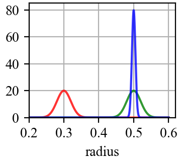
(a)

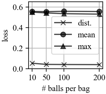
(b)

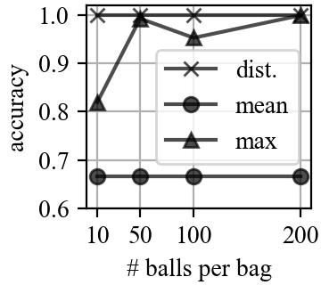
(c)

Figure 2: 3-class MIL classification task: classifying bags of metal balls from 3 different production lines. (a) Distribution of radius of balls produced in red, green and blue production lines. (b) Loss and (c) accuracy values of MIL models with ‘distribution’ (dist.) pooling, ‘mean’ pooling and ‘max’ pooling filters on the test set bags with 10, 50, 100 and 200 balls per bag.

We generated radius data for 900 bags of metal balls with corresponding production line labels. There were 300 bags from each production line and each bag had 200 balls. We designed an MIL framework such that a bag level representation was obtained by using an MIL pooling filter over the radius values of the balls in a bag. Then, the bag level representation was fed to a linear classifier to predict the production line label of the bag. We splitted data into training, validation and test sets with 600, 150 and 150 bags, respectively. In each set, there are equal number of bags from each class. We trained MIL models with ‘distribution’, ‘mean’ and ‘max’ pooling filters on the bags with 10, 50, 100 and 200 balls per bag. All models were trained on the training set with categorical cross-entropy loss and fine-tuned on the validation set. Loss and accuracy values of the models on the test set are given in Figure 2(b) and 2(c), respectively. As it is seen in Figure 2(c), models with ‘distribution’ pooling classified all the bags perfectly by exploiting the full information in the radius distribution of balls in the bags and outperformed the models with ‘mean’ and ‘max’ pooling. While models with ‘mean’ pooling distinguished bags of red line from others, it couldn’t distinguish the bags of green line from the bags of blue line since their mean radius values were close to each other. For models with ‘max’ pooling, they can distinguish bags of red line from others. For bags from green and blue lines, the ‘max’ polling can distinguish them only when the number of balls inside the bags is big enough. Moreover, loss of models with ‘distribution’ pooling is much lower than the others, so they are much more confident in their predictions. (See Supp. 2 for details.)

4.3 Performance comparison on classical MIL datasets

This section compares the performance of our neural network model with ‘distribution’ pooling filter (Distribution-Net) with the performance of the best MIL methods on classical MIL task of positive vs negative bag classification on 5 classical MIL datasets: drug activity prediction datasets MUSK1 and MUSK2 [2] and animal image annotation datasets FOX, TIGER and ELEPHANT [8]. A drug is usually a small molecule that works by binding to a target protein molecule and may have multiple conformations. In MUSK datasets, each drug is represented as a bag of feature vectors obtained from its conformations and a label showing whether any of the conformations of the drug binds to its target protein (positive) or not (negative) is provided. Similarly, in animal datasets, each image is represented as a bag of feature vectors extracted from segments of the image and a label showing whether the image contains the particular animal (positive) or not (negative) is provided. (See Supp. 3 for details of models and datasets.)

We used 10-fold cross validation and repeated each experiment 5 times. For each dataset, we have declared the mean of classification accuracies ($\pm$ standard error). We compared the performance of our neural network model with ‘distribution’ pooling filter with the performance of state-of-the-art MIL methods on classical MIL datasets in Table 3. While first part of the table contains methods utilizing traditional machine learning techniques [8, 19, 9, 23, 50], second part of the table accommodates methods employing neural networks [10, 11]. The last part of the table shows the performance of our own model with ‘distribution’ pooling filter (Distribution-Net), which outperformed all other methods on all datasets. While neural network based models generally outperformed the traditional machine learning based models, it seems that our Distribution-Net utilized the power of its ‘distribution’ pooling filter over other neural network based models.

Table 3: Performances of different MIL methods on classical MIL datasets. First part: methods utilizing traditional machine learning techniques. Second part: methods employing neural networks. Last part: our own model with ‘distribution’ pooling filter (Distribution-Net).

METHOD	MUSK1	MUSK2	FOX	TIGER	ELEPHANT
mi-SVM [8]	0.874 $\pm$ N/A	0.836 $\pm$ N/A	0.582 $\pm$ N/A	0.784 $\pm$ N/A	0.822 $\pm$ N/A
MI-SVM [8]	0.779 $\pm$ N/A	0.843 $\pm$ N/A	0.578 $\pm$ N/A	0.840 $\pm$ N/A	0.843 $\pm$ N/A
MI-Kernel [19]	0.880 $\pm$ 0.031	0.893 $\pm$ 0.015	0.603 $\pm$ 0.028	0.842 $\pm$ 0.010	0.843 $\pm$ 0.016
EM-DD [9]	0.849 $\pm$ 0.044	0.869 $\pm$ 0.048	0.609 $\pm$ 0.045	0.730 $\pm$ 0.043	0.771 $\pm$ 0.043
mi-Graph [23]	0.889 $\pm$ 0.033	0.903 $\pm$ 0.039	0.620 $\pm$ 0.044	0.860 $\pm$ 0.037	0.869 $\pm$ 0.035
miVLAD [50]	0.871 $\pm$ 0.043	0.872 $\pm$ 0.042	0.620 $\pm$ 0.044	0.811 $\pm$ 0.039	0.850 $\pm$ 0.036
miFV [50]	0.909 $\pm$ 0.040	0.884 $\pm$ 0.042	0.621 $\pm$ 0.049	0.813 $\pm$ 0.037	0.852 $\pm$ 0.036
mi-Net [10]	0.889 $\pm$ 0.039	0.858 $\pm$ 0.049	0.613 $\pm$ 0.035	0.824 $\pm$ 0.034	0.858 $\pm$ 0.037
MI-Net [10]	0.887 $\pm$ 0.041	0.859 $\pm$ 0.046	0.622 $\pm$ 0.038	0.830 $\pm$ 0.032	0.862 $\pm$ 0.034
MI-Net with DS [10]	0.894 $\pm$ 0.042	0.874 $\pm$ 0.043	0.630 $\pm$ 0.037	0.845 $\pm$ 0.039	0.872 $\pm$ 0.032
MI-Net with RC [10]	0.898 $\pm$ 0.043	0.873 $\pm$ 0.044	0.619 $\pm$ 0.047	0.836 $\pm$ 0.037	0.857 $\pm$ 0.040
Attention [11]	0.892 $\pm$ 0.040	0.858 $\pm$ 0.048	0.615 $\pm$ 0.043	0.839 $\pm$ 0.022	0.868 $\pm$ 0.022
Gated-Attention [11]	0.900 $\pm$ 0.050	0.863 $\pm$ 0.042	0.603 $\pm$ 0.029	0.845 $\pm$ 0.018	0.857 $\pm$ 0.027
Distribution-Net (ours)	0.923 $\pm$ 0.071	0.932 $\pm$ 0.067	0.680 $\pm$ 0.075	0.864 $\pm$ 0.054	0.900 $\pm$ 0.077

5 Conclusion

In this paper, we investigated the effect of different MIL pooling filters on the performance of an MIL model in some real world MIL tasks. We designed a neural network based MIL framework and analyzed the performance of our framework with 5 different MIL pooling filters in 5 different MIL tasks formulated on the lymph node metastases dataset. We observed that while the performance of our framework in a particular MIL task is different for different MIL pooling filters, the performance of our framework with a specific MIL pooling filter also changes from task to task. Thus, we conclude that choosing a correct MIL pooling filter for an MIL task is crucial for better performance. Furthermore, we noticed that although it is not the best performing MIL pooling filter for all tasks, ‘distribution with attention’ pooling filter seems to be a good candidate for almost all MIL tasks. Actually, this is in accordance with our theoretical assertion in Sec. 2.2 that ‘distribution’ based pooling filters capture richer information than point estimate based counterparts. While our model with ‘distribution’ pooling outperformed its counterparts with ‘mean’ and ‘max’ pooling in bag of metal balls classification experiment (Sec. 4.2), it also outperformed state-of-the art methods with different MIL pooling filters on classical MIL datasets (Sec. 4.3). On top of observed superiority of ‘distribution’ based pooling filters, in future, we want to explore them with fully trainable hyper-parameters, such as number of bins and standard deviation.

Supplementary Materials

1    Experiments on lymph node metastases dataset

We investigated the effect of MIL pooling filter on the performance of an MIL model in a particular real world MIL task. We designed a neural network based MIL framework and analyzed the performance of our framework with 5 different MIL pooling filters in 5 different MIL tasks formulated on a real world lymph node metastases dataset.

Code for the experiments was made publicly available at: https://bit.ly/mil_pooling_filters

1.1    Lymph node metastases dataset

The lymph node metastases dataset is adapted from [4]. The original dataset consists of $512\times 512$ images cropped from histopathology slides of lymph node sections [16] and has corresponding ground truth metastases segmentation masks. There are three types of images in this dataset: fully normal - all cells are normal, fully metastases - all cells are metastases and boundary - mixture of normal and metastases cells. In order to make a clear distinction between these three types of images, we filtered out the images with: (i) $0<\text{percent metastases}\leq 20$ and (ii) $80\leq\text{percent metastases}<100$. Moreover, in order to obtain a balanced dataset, we dropped some of the images in the test set coming from one specific slide. The script to obtain our dataset from the original dataset in [4] is also inside the code folder.

Our dataset is publicly available with this paper. For our dataset, number of images and percent metastases histograms in training, validation and test sets are given in Table 4 and Figure 3, respectively.

Table 4: Lymph node metastases dataset - number of images in training, validation and test sets.

	Fully normal	Fully metastases	Boundary	Total
Training	395	228	310	933
Validation	267	190	211	668
Test	277	231	228	736

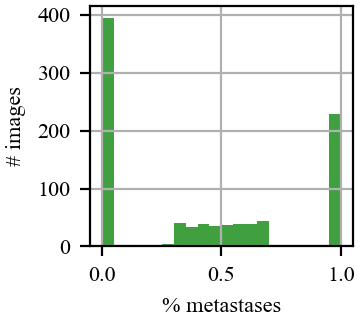
(a) Training

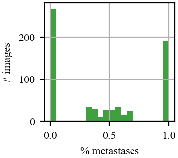
(b) Validation

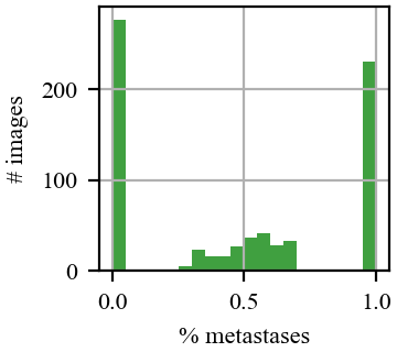
(c) Test

Figure 3: Percent metastases histograms for training, validation and test sets.

1.2    Neural network architectures and hyper-parameters

We designed a neural network based MIL framework. We used ResNet18 [44] architecture without batch normalization as feature extractor module, $\theta_{\mbox{\tiny feature}}$, and a three layer multi-layer-perceptron as bag level representation transformation module, $\theta_{\mbox{\tiny transform}}$. We tested this framework with 5 different MIL pooling filters in $\operatorname*{\theta_{\mbox{\tiny filter}}}$ module on 5 different MIL tasks formulated. Hence, we had 25 different models sharing the same architecture in $\theta_{\mbox{\tiny feature}}$ module. Moreover, all models have the same hidden layers in $\theta_{\mbox{\tiny transform}}$ module; however, note that number of input nodes in $\theta_{\mbox{\tiny transform}}$ module depends on $\operatorname*{\theta_{\mbox{\tiny filter}}}$ and number of output nodes in $\theta_{\mbox{\tiny transform}}$ module depends on MIL task. Please refer to the provided code for more details.

During training of the models, each image was treated as a bag. We prepared bags on-the-go during training by randomly cropping $32\times 32$ patches over the images. Each bag was created with 64 cropped patches (instances). Data augmentation was also applied on the cropped patches. We used batch size of 32 and extracted 32 features for each instance inside a bag. In the models with ‘distribution’ pooling filter, kernel density estimation with a Gaussian kernel was used to estimate marginal distributions of extracted features. We used standard deviation of $\sigma=0.0167$ in Gaussian kernel and 21 bins to sample the estimated distributions. Furthermore, for attention mechanism, we used the same architecture in [11] in the models with ‘attention’ pooling and ‘distribution with attention’ pooling filters. We trained models by using ADAM optimizer with a learning rate of $lr=1e-4$ and $L2$ regularization on the weights with a weight decay of $weight\_decay=0.0005$. Each model was randomly initialized and trained end-to-end with early-stopping criteria on validation set performance. List of hyper-parameters used in MIL models is given in Table 5.

During testing, we created 100 bags from each image and tested with the trained model. Final label for each image in the test set was obtained by averaging 100 predictions.

Table 5: Experiments on lymph node metastases dataset - architecture and list of hyper-parameters used in the MIL models. ‘dist_w_att’: ‘distribution with attention’ pooling

	input-$32x32x3$
	ResNet18 w/o BN
	‘distribution’ / ‘dist_w_att’ / ‘mean’ / ‘attention’ / ‘max’ pooling
	Dropout(0.5)
	fc-128 + ReLU
Architecture	Dropout(0.5)
	fc-32 + ReLU
	Dropout(0.5)
	fc-2 (+ve/-ve, ucc, 2-task) / fc-3 (3-class) / fc-1 (regression)
	softmax (+ve/-ve, ucc, 3-class) / sigmoid (2-task) / None (regression)
image size	$512\times 512$
patch size	$32\times 32$
# instances per bag	64
# features	32
# bins in ‘distribution’ filters	21
$\sigma$ in Gaussian kernel	0.0167
Optimizer	ADAM
Learning rate	$1e-4$
$L2$ regularization weight decay	0.0005
batch size	32

2    Experiments on bags of metal balls

‘Distribution’ pooling extracts full information of the distribution. However, ‘mean’ and ‘max’ pooling only provide point estimates. This experiment aims to show that ‘distribution’ pooling is more powerful than point estimators like ‘mean’ and ‘max’ pooling. We have a hypothetical factory producing metal balls for ball bearings. The factory has three production lines, namely red, green and blue, and radius of the balls produced in these lines are normally distributed: $r_{red}\sim\mathcal{N}(\mu=0.3,\sigma=0.02)$, $r_{green}\sim\mathcal{N}(\mu=0.5,\sigma=0.02)$ and $r_{blue}\sim\mathcal{N}(\mu=0.5,\sigma=0.005)$. Then, our MIL task is to classify bags of metal balls from 3 different production lines, i.e. 3-class MIL classification task.

We designed an MIL framework such that a bag level representation was obtained by using an MIL pooling filter over the radius values of the balls in a bag. Then, the bag level representation was fed to a linear classifier to predict the production line label of the bag. List of hyper-parameters used in MIL models is given in Table 6.

Table 6: Classifying bags of metal balls - architecture and list of hyper-parameters used in the MIL models.

	input-1
Architecture	‘mean’ / ‘max’ / ‘distribution’ pooling
	fc-3
	softmax
# balls per bag	10 / 50 / 100 / 200
# features	1
# bins in ‘distribution’ pooling filters	101
$\sigma$ in Gaussian kernel	0.005
Optimizer	ADAM
Learning rate	$1e-2$
$L2$ regularization weight decay	0.0005
batch size	64

Figure 4, shows test set confusion matrices. Models with ‘distribution’ pooling classified all the bags perfectly by exploiting the full information in the radius distribution of balls in the bags and outperformed the models with ‘mean’ and ‘max’ pooling. While models with ‘mean’ pooling distinguished bags of red line from others, it couldn’t distinguish the bags of green line from the bags of blue line since their mean radius values were close to each other. For models with ‘max’ pooling, they can distinguish bags of red line from others. For bags from green and blue lines, the ‘max’ polling can distinguish them only when the number of balls inside the bags is big enough.

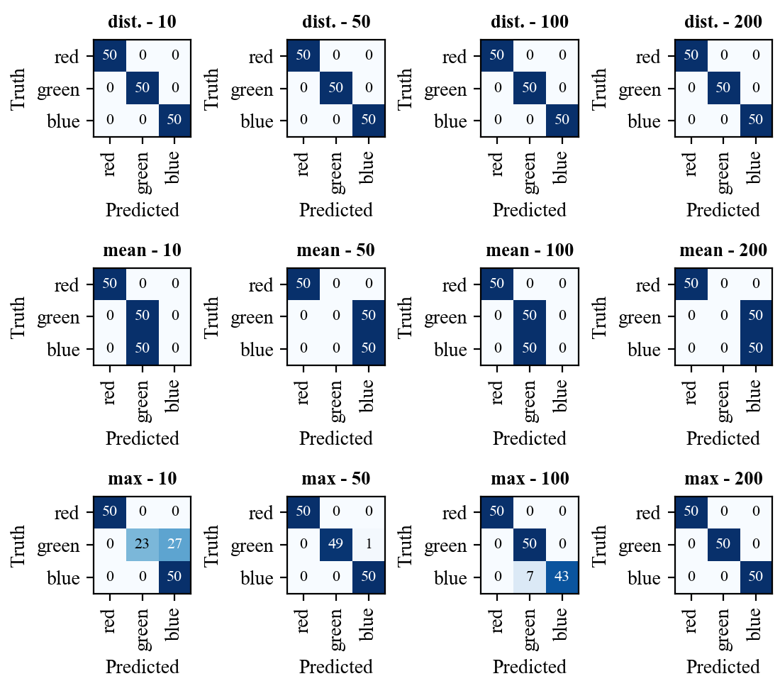
Figure 4: Confusion matrices for models with ‘distribution’ (dist.) pooling, ‘mean’ pooling and ‘max’ pooling filters on the test set bags with 10, 50, 100 and 200 balls per bag.

3    Experiments on classical MIL datasets

This section compares the performance of our neural network model with ‘distribution’ pooling filter (Distribution-Net) with the performance of the best MIL methods on classical MIL task of positive vs negative bag classification on 5 classical MIL datasets: drug activity prediction datasets MUSK1 and MUSK2 [2] and animal image annotation datasets FOX, TIGER and ELEPHANT [8]. Summary of classical MIL datasets is given in Table 7.

Table 7: Summary of classical MIL datasets

	# bags			# instances per bag
	positive	negative	total	min	max	average	# features
MUSK1	47	45	92	2	40	5.17	166
MUSK2	39	63	102	1	1044	64.69	166
FOX	100	100	200	2	13	6.6	230
TIGER	100	100	200	1	13	6.1	230
ELEPHANT	100	100	200	2	13	6.96	230

The summary of architectures and hyper-parameters used in MIL models on ‘MUSK’ and ‘Animal’ datasets are given in Table 8 and Table 9, respectively. Note that we used mini-batch training with bags including equal number of instances. We created bags by sampling from available instances of each sample (a drug with multiple conformations for ‘MUSK’ datasets and an image with multiple segments in ‘Animal’ datasets). When the number of available instances of a sample is less than number of instances required to create a bag we used available instances more than once in a bag.

Table 8: MUSK datasets - architecture and list of hyper-parameters used in the MIL models.

	input-166
	fc-64 + ReLU
	Dropout(0.5)
	fc-32 + ReLU
	Dropout(0.5)
	fc-32 + Sigmoid
Architecture	‘distribution’ pooling
	Dropout(0.5)
	fc-64 + ReLU
	Dropout(0.5)
	fc-32 + ReLU
	Dropout(0.5)
	fc-2
	softmax
# instances per bag	16
# features	32
# bins in ‘distribution’ pooling filters	11
$\sigma$ in Gaussian kernel	0.1
Optimizer	ADAM
Learning rate	$5e-4$
$L2$ regularization weight decay	0.1
batch size	8

Table 9: Animal datasets - architecture and list of hyper-parameters used in the MIL models.

	input-230
	fc-256 + ReLU
	Dropout(0.5)
	fc-128 + ReLU
	Dropout(0.5)
	fc-64 + ReLU
	Dropout(0.5)
	fc-32 + Sigmoid
Architecture	‘distribution’ pooling
	Dropout(0.5)
	fc-384 + ReLU
	Dropout(0.5)
	fc-192 + ReLU
	Dropout(0.5)
	fc-2
	softmax
# instances per bag	16
# features	32
# bins in ‘distribution’ pooling filters	11
$\sigma$ in Gaussian kernel	0.1
Optimizer	Adam
Learning rate	$5e-6$
$L2$ regularization weight decay	0.1
batch size	8

References

- [1] W. Zhu, Q. Lou, Y. S. Vang, and X. Xie, “Deep multi-instance networks with sparse label assignment for whole mammogram classification,” in International Conference on Medical Image Computing and Computer-Assisted Intervention, pp. 603–611, Springer, 2017.
- [2] T. G. Dietterich, R. H. Lathrop, and T. Lozano-Pérez, “Solving the multiple instance problem with axis-parallel rectangles,” Artificial intelligence, vol. 89, no. 1-2, pp. 31–71, 1997.
- [3] O. Maron and T. Lozano-Pérez, “A framework for multiple-instance learning,” in Advances in neural information processing systems, pp. 570–576, 1998.
- [4] M. U. Oner, H. K. Lee, and W.-K. Sung, “Weakly supervised clustering by exploiting unique class count,” in International Conference on Learning Representations, 2020.
- [5] J. Feng and Z.-H. Zhou, “Deep miml network,” in Thirty-First AAAI Conference on Artificial Intelligence, 2017.
- [6] Y. Yang, C. Deng, S. Gao, W. Liu, D. Tao, and X. Gao, “Discriminative multi-instance multitask learning for 3d action recognition,” IEEE Transactions on Multimedia, vol. 19, no. 3, pp. 519–529, 2016.
- [7] Y. Zhang, R. Zhao, W. Dong, B.-G. Hu, and Q. Ji, “Bilateral ordinal relevance multi-instance regression for facial action unit intensity estimation,” in Proceedings of the IEEE Conference on Computer Vision and Pattern Recognition, pp. 7034–7043, 2018.
- [8] S. Andrews, I. Tsochantaridis, and T. Hofmann, “Support vector machines for multiple-instance learning,” in Advances in neural information processing systems, pp. 577–584, 2003.
- [9] Q. Zhang and S. A. Goldman, “Em-dd: An improved multiple-instance learning technique,” in Advances in neural information processing systems, pp. 1073–1080, 2002.
- [10] X. Wang, Y. Yan, P. Tang, X. Bai, and W. Liu, “Revisiting multiple instance neural networks,” Pattern Recognition, vol. 74, pp. 15–24, 2018.
- [11] M. Ilse, J. Tomczak, and M. Welling, “Attention-based deep multiple instance learning,” in International Conference on Machine Learning, pp. 2127–2136, 2018.
- [12] J. Wu, Y. Yu, C. Huang, and K. Yu, “Deep multiple instance learning for image classification and auto-annotation,” in Proceedings of the IEEE Conference on Computer Vision and Pattern Recognition, pp. 3460–3469, 2015.
- [13] Y. Wang, J. Li, and F. Metze, “A comparison of five multiple instance learning pooling functions for sound event detection with weak labeling,” in ICASSP 2019-2019 IEEE International Conference on Acoustics, Speech and Signal Processing (ICASSP), pp. 31–35, IEEE, 2019.
- [14] J. Ramon and L. De Raedt, “Multi instance neural networks,” 2000.
- [15] A. Dang, T. H. Vu, and J.-C. Wang, “Deep learning for dcase2017 challenge,” in Workshop on DCASE2017 Challenge, Tech. Rep, 2017.
- [16] B. E. Bejnordi, M. Veta, P. J. Van Diest, B. Van Ginneken, N. Karssemeijer, G. Litjens, J. A. Van Der Laak, M. Hermsen, Q. F. Manson, M. Balkenhol, et al., “Diagnostic assessment of deep learning algorithms for detection of lymph node metastases in women with breast cancer,” Jama, vol. 318, no. 22, pp. 2199–2210, 2017.
- [17] E. Parzen, “On estimation of a probability density function and mode,” The annals of mathematical statistics, vol. 33, no. 3, pp. 1065–1076, 1962.
- [18] N. Quadrianto, A. J. Smola, T. S. Caetano, and Q. V. Le, “Estimating labels from label proportions,” Journal of Machine Learning Research, vol. 10, no. Oct, pp. 2349–2374, 2009.
- [19] T. Gärtner, P. A. Flach, A. Kowalczyk, and A. J. Smola, “Multi-instance kernels,” in ICML, vol. 2, p. 7, 2002.
- [20] Y. Chen, J. Bi, and J. Z. Wang, “Miles: Multiple-instance learning via embedded instance selection,” IEEE Transactions on Pattern Analysis and Machine Intelligence, vol. 28, no. 12, pp. 1931–1947, 2006.
- [21] J. R. Foulds, Learning instance weights in multi-instance learning. PhD thesis, The University of Waikato, 2008.
- [22] M.-L. Zhang and Z.-H. Zhou, “Multi-instance clustering with applications to multi-instance prediction,” Applied Intelligence, vol. 31, no. 1, pp. 47–68, 2009.
- [23] Z.-H. Zhou, Y.-Y. Sun, and Y.-F. Li, “Multi-instance learning by treating instances as non-iid samples,” in Proceedings of the 26th annual international conference on machine learning, pp. 1249–1256, ACM, 2009.
- [24] Z.-H. Zhou and M.-L. Zhang, “Neural networks for multi-instance learning,” in Proceedings of the International Conference on Intelligent Information Technology, Beijing, China, pp. 455–459, 2002.
- [25] M.-L. Zhang and Z.-H. Zhou, “Improve multi-instance neural networks through feature selection,” Neural Processing Letters, vol. 19, no. 1, pp. 1–10, 2004.
- [26] J. Foulds and E. Frank, “A review of multi-instance learning assumptions,” The Knowledge Engineering Review, vol. 25, no. 1, pp. 1–25, 2010.
- [27] Y. Chen and J. Z. Wang, “Image categorization by learning and reasoning with regions,” Journal of Machine Learning Research, vol. 5, no. Aug, pp. 913–939, 2004.
- [28] Q. Zhang, S. A. Goldman, W. Yu, and J. E. Fritts, “Content-based image retrieval using multiple-instance learning,” in ICML, vol. 1, p. 2, Citeseer, 2002.
- [29] J. Tang, H. Li, G.-J. Qi, and T.-S. Chua, “Image annotation by graph-based inference with integrated multiple/single instance representations,” IEEE Transactions on Multimedia, vol. 12, no. 2, pp. 131–141, 2010.
- [30] B. Settles, M. Craven, and S. Ray, “Multiple-instance active learning,” in Advances in neural information processing systems, pp. 1289–1296, 2008.
- [31] Z. Jorgensen, Y. Zhou, and M. Inge, “A multiple instance learning strategy for combating good word attacks on spam filters,” Journal of Machine Learning Research, vol. 9, no. Jun, pp. 1115–1146, 2008.
- [32] M. Dundar, B. Krishnapuram, R. Rao, and G. M. Fung, “Multiple instance learning for computer aided diagnosis,” in Advances in neural information processing systems, pp. 425–432, 2007.
- [33] G. Quellec, G. Cazuguel, B. Cochener, and M. Lamard, “Multiple-instance learning for medical image and video analysis,” IEEE reviews in biomedical engineering, vol. 10, pp. 213–234, 2017.
- [34] C. Zhang, J. C. Platt, and P. A. Viola, “Multiple instance boosting for object detection,” in Advances in neural information processing systems, pp. 1417–1424, 2006.
- [35] P. F. Felzenszwalb, R. B. Girshick, D. McAllester, and D. Ramanan, “Object detection with discriminatively trained part-based models,” IEEE transactions on pattern analysis and machine intelligence, vol. 32, no. 9, pp. 1627–1645, 2010.
- [36] B. Babenko, M.-H. Yang, and S. Belongie, “Robust object tracking with online multiple instance learning,” IEEE transactions on pattern analysis and machine intelligence, vol. 33, no. 8, pp. 1619–1632, 2011.
- [37] C. Kou, H. K. Lee, E.-C. Chang, and T. K. Ng, “Enhancing transformation-based defenses against adversarial attacks with a distribution classifier,” in International Conference on Learning Representations, 2020.
- [38] M. Zaheer, S. Kottur, S. Ravanbakhsh, B. Poczos, R. R. Salakhutdinov, and A. J. Smola, “Deep sets,” in Advances in neural information processing systems, pp. 3391–3401, 2017.
- [39] S. H. Rezatofighi, A. Milan, E. Abbasnejad, A. Dick, I. Reid, et al., “Deepsetnet: Predicting sets with deep neural networks,” in 2017 IEEE International Conference on Computer Vision (ICCV), pp. 5257–5266, IEEE, 2017.
- [40] L. I. Kuncheva, J. J. Rodríguez, and A. S. Jackson, “Restricted set classification: Who is there?,” Pattern Recognition, vol. 63, pp. 158–170, 2017.
- [41] J. Lee, Y. Lee, J. Kim, A. Kosiorek, S. Choi, and Y. W. Teh, “Set transformer: A framework for attention-based permutation-invariant neural networks,” in International Conference on Machine Learning, pp. 3744–3753, 2019.
- [42] X. Lu, Z. Lin, X. Shen, R. Mech, and J. Z. Wang, “Deep multi-patch aggregation network for image style, aesthetics, and quality estimation,” in Proceedings of the IEEE International Conference on Computer Vision, pp. 990–998, 2015.
- [43] Y. Zhang, J. Hare, and A. Prügel-Bennett, “Fspool: Learning set representations with featurewise sort pooling,” in International Conference on Learning Representations, 2020.
- [44] K. He, X. Zhang, S. Ren, and J. Sun, “Deep residual learning for image recognition,” in Proceedings of the IEEE conference on computer vision and pattern recognition, pp. 770–778, 2016.
- [45] “PyTorch cross entropy loss function.” https://pytorch.org/docs/stable/nn.html#crossentropyloss. Accessed: 2020-05-28.
- [46] “PyTorch binary cross entropy loss function.” https://pytorch.org/docs/stable/nn.html#bcewithlogitsloss. Accessed: 2020-05-28.
- [47] B. Everitt, “The analysis of contingency tables,” 1977.
- [48] T. G. Dietterich, “Approximate statistical tests for comparing supervised classification learning algorithms,” Neural computation, vol. 10, no. 7, pp. 1895–1923, 1998.
- [49] H. Hsu and P. A. Lachenbruch, “Paired t test,” Encyclopedia of Biostatistics, vol. 6, 2005.
- [50] X.-S. Wei, J. Wu, and Z.-H. Zhou, “Scalable algorithms for multi-instance learning,” IEEE transactions on neural networks and learning systems, vol. 28, no. 4, pp. 975–987, 2016.