Heavy quark correlators in Instanton Liquid Model with perturbative corrections

Abstract

In the present work we consider the influence on the heavy quark correlators due to the instanton background in the framework of instanton liquid model (ILM) of QCD vacuum by taking into account also the perturbative gluon effects. For a single heavy quark this leads to the mass shift due to the direct-instanton nonperturbative and ILM modified perturbative contributions, respectively. In the heavy quark-antiquark ($Q\bar{Q}$) sector we obtain the potential consisting the direct instanton induced part and the one-gluon exchange (OGE) perturbative part which is screened at large distances due to the nonperturbative dynamics. At the region of interest corresponding to the heavy quark physics the screening effect in OGE can be well approximated by a Yukawa-type potential in terms of the dynamically generated gluon mass. A possible implication of the present studies to the phenomenology of heavy quarkonium is also discussed.

I Introduction

The properties of heavy quarkonium $Q\bar{Q}$ (a colorless system consisting a heavy quark $Q$ and another heavy antiquark $\bar{Q}$) in the framework of phenomenological approaches can be well described essentially on a basis of non-relativistic potential models. The model quite popular among them is one with so-called Cornell potential Eichten:1974af , which has a nature of Coulomb-like attractive part at short distances and linear confining part at long distances. The form of potential is given as

$$V_{\rm Cornell}(r)=\frac{\kappa}{r}+\sigma r\,,$$ (1)

where the Coulomb coupling $\kappa<0$ and the string constant $\sigma>0$. The short-distance behavior of quantum chromodynamics (QCD) is dominated by the one-gluon exchange interaction and the corresponding potential can be calculated perturbatively. At the leading order on the strong coupling constant $\alpha_{s}=g^{2}/(4\pi)$, one reproduces the first term in Eq. (1) with the constant $\kappa=-(4/3)\alpha_{s}$ where ‘$-4/3$’ is color factor corresponding to the color singlet $Q\bar{Q}$ state. Nevertheless, in the practical calculations $\kappa$ is mostly considered as a pure phenomenological parameter.

The confining part of the potential is pure phenomenological one due to the fact that we do not fully understand yet the mechanism of confinement. Therefore, some authors are using the harmonic oscillator type $\sim r^{2}$ or the logarithmic $\sim\ln(r)$ dependencies for the confining part of potential. From other side, the lattice QCD calculations showed the linear $\sim r$ dependence of the full potential at large distances (see, e.g. Ref. Bali:2000gf ) supporting in such a way the Cornell-type form of potentials. Actually, all these potential models with the different confining forms reasonable well match with the data due to the reason that they do not much affect at short distances where we have the sensitive probes. This kind of common behavior of different confining potentials at the short distances is also partial reason for considering the Coulomb-coupling $\kappa$ as a pure phenomenological parameter.

In principle, one can further try to develop the potential approach and improve the description of data by taking into account the relativistic and perturbative corrections on the strong coupling constant $\alpha_{s}$ of QCD Brambilla:2009bi ; Mateu:2018zym . However, the more influential effects may still be hidden behind of the non-perturbative structure of QCD vacuum. Therefore, one should develop the more general systematic approach which takes into account not only the next order perturbative effects but also the nonperturbative effects in the properties of heavy quark systems.

Here it is necessary to note, that the light quark sector of hadronic physics is successfully described by means of spontaneous breakdown of chiral symmetry in the framework of instanton liquid model of QCD vacuum (ILM) (see reviews Diakonov:2002fq ; Schafer:1996wv ; shuryak2018 and Refs. Goeke:2007bj ; Goeke:2007nc ; Goeke:2010hm ; Musakhanov:2012zm ; Musakhanov:2018sdu ). One may also expect that the non-perturbative effects on the heavy quark propagation in the instanton medium still may be substantial at last but not least. Consequently, our aim in the present work is development of the systematic accounting scheme for the instanton effects during the calculations of heavy quark correlators. By doing this, we will work in the framework of the ILM and simultaneously consider the perturbative gluon contributions.

The paper is organized in the following way. In the next Section II we discuss an applicability of ILM in the heavy quark sector by comparing the parameters of ILM with the quark core sizes of hadrons. Then in Section III, we explain the formalism of calculations of the heavy quark correlators in the instanton medium by accounting also the perturbative gluon corrections. Section IV is devoted to the calculations of heavy quark propagator in ILM and estimations of the possible contributions to the heavy quark mass. Further, two body heavy quark-antiquark correlator in ILM is presented in Section V. In particular, the results corresponding to the heavy quark potential are discussed in Subsections V.1 and V.2. In Section VI we will analyse the order of instanton effects in the quarkonium spectra and will make the corresponding conclusions. Finally, in Section VII the present studies and the outlook for future investigations will be summarized. The details of the calculations of the heavy quark correlators with the perturbative gluon corrections in ILM are given in the Appendix A.

II ILM parameters vs hadron quark core sizes

QCD vacuum has the rich topological structures and, probably, the most important among them is an instanton – a classical solution of Yang-Mills equations in the 4-dimensional Euclidean space. The vacuum of QCD has a degenerate and periodic structure in the functional space along the collective coordinate direction which is called the Chern-Simons (CS) coordinate. Therefore, QCD vacuum can be considered as the lowest energy quantum state of the one-dimensional crystal along the CS coordinate FJR1976 ; Jackiw:1976pf . The QCD instanton (anti-instanton) is a tunneling mechanism in forward (backward) direction between the different Chern-Simons states corresponding to the degenerate vacuum Belavin:1975fg . The (anti)instanton is described by its collective coordinates denoted as $\xi_{I}$: the position in 4-dimensional Euclidean space $z_{I}$, the instanton size $\rho_{I}$ and the SU$(N_{c})$ color orientation given by the unitary matrix $U_{I}$, $4N_{c}$ variables altogether. The main parameters of ILM are the average instanton size $\bar{\rho}$ and the inter-instanton distance $R$, or the density of instanton media $N/V\equiv 1/R^{4}$ given in terms of the inter-instanton distance (see reviews Diakonov:2002fq ; Schafer:1996wv ; shuryak2018 ). Phenomenologically, their values were estimated as

$$\bar{\rho}=\frac{1}{3}\,{\rm fm},\qquad R=1\,{\rm fm}.$$ (2)

These values were found to be in general reasonably and confirmed by the theoretical variational calculations Diakonov:2002fq ; Schafer:1996wv ; shuryak2018 and the lattice simulations of the QCD vacuum Chu:1994vi ; Negele:1998ev ; DeGrand:2001tm ; Faccioli:2003qz .

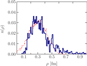
Figure 1: (Color online) Dependence of the instanton size distribution function $n$ on the instanton size parameter $\rho$: the dots correspond to the ILM and the continuous lines correspond to the lattice simulations Millo:2011zn .

From other side, the instanton size distribution $n(\rho)$ has also been studied by lattice simulations Millo:2011zn (see Fig.1). As we can see, for the relatively large-size instantons ($\rho\sim R$) the distribution function $n(\rho)$ is suppressed. Therefore, a simple sum-ansatz for the total instanton field $A(\xi)=\sum_{i}A_{i}(\xi_{i})$ expressed in terms of the single instanton solutions $A_{i}(\xi_{i})$ is quite well justified during the practical applications. Nevertheless, the the large-size tail of distribution function $n(\rho)$ becomes important in the confinement regime of QCD. Here one should replace BPST instantons by KvBLL instantons Kraan:1998kp ; Kraan:1998pm ; Lee:1998bb described in terms of dyons. In such a way, one gets an extension of ILM – liquid dyon model (LDM) Diakonov:2009jq ; Liu:2015ufa ; Liu:2015jsa , which is able to reproduce confinement–deconfinement phases. Consequently, the small size instantons can still be described in terms of their collective coordinates. For comparison, we remind that the average size of instantons in LDM is $\bar{\rho}\approx 0.5\,{\rm fm}$ Diakonov:2009jq ; Liu:2015ufa ; Liu:2015jsa , while in ILM $\bar{\rho}\approx 0.3\,{\rm fm}$. Hereafter, we will neglect the effect of size distribution’s width and simply consider the instanton size $\rho$ equal to its average value, $\rho=\bar{\rho}$.

At the typical values of the ILM parameters given  in Eq. (2), the instanton background leads to the nonzero QCD vacuum energy density $\epsilon\approx-500\,{\rm MeV/fm^{3}}$ Schafer:1996wv ; shuryak2018 and it occurs a spontaneous breakdown of chiral symmetry which plays the pivotal and significant role in describing the lightest hadrons and their interactions. In such a way, ILM succeeded to explain the hadron physics at the light quark sector (see reviews Diakonov:2002fq ; Schafer:1996wv ; shuryak2018 and Refs. Goeke:2007bj ; Goeke:2007nc ; Goeke:2010hm ; Musakhanov:2012zm ; Musakhanov:2018sdu ).

In order to understand the applicability of ILM in the heavy quark sector, one may pay an attention that the typical sizes of quarkonia are relatively small Digal:2005ht ; Eichten:1979ms . In particular, the smallness in size is more pronounced in the case of low laying states, e.g. see $r_{J/\psi}$ and $r_{\Upsilon}$ in the Table 1.

Table 1: Masses and sizes of quarkonium states in the non-relativistic potential model Digal:2005ht .

Characteristics	Charmonia			Bottomonia
of states	$J/\psi$	$\chi_{c}$	$\psi^{\prime}$	$\Upsilon$	$\chi_{b}$	$\Upsilon^{\prime}$	$\chi_{b}^{\prime}$	$\Upsilon^{{}^{\prime\prime}}$
mass [GeV]	3.07	3.53	3.68	9.46	9.99	10.02	10.26	10.36
size $r$ [fm]	0.25	0.36	0.45	0.14	0.22	0.28	0.34	0.39

A similar estimate of nucleon’s quark core size gives the result $r_{N}\sim 0.3-0.5$ fm He:1986yq ; Weise ; Tegen . Due to the fact, that the quark core of hadrons are relatively small in size, one may conclude that they are insensitive to the confinement mechanism. Consequently, ILM may be safely applied for the description of hadron properties at the heavy quark sector too. However, one should take care about the perturbative effects during the analysis of heavy hadrons’ spectra and we will keep it in mind during our calculations.

III Heavy quark correlators with perturbative corrections

As we discussed above, in ILM the background field due to instantons is given by a simple sum $A(\xi)=\sum_{i}A_{i}(\xi_{i})$, where $\xi_{i}=(z_{i},U_{i},\rho_{i})$ are collective coordinates of instantons. It is also necessary to note that the instanton field has specific strong coupling dependence given as $A\sim 1/g$. The corresponding partition function in ILM $Z[j]$ (it is normalized as $Z[0]=1$) with account of perturbative gluons $a_{\mu}$ and their sources $j_{\mu}$ is approximated by the expression

$$Z[j] =\int D\xi Dae^{-[S_{eff}[a,A(\xi)]+(ja)]}$$ (3)

$$\approx\int D\xi e^{-\frac{1}{2}(j_{\mu}S_{\mu\nu}(\xi)j_{\nu})},$$ (4)

where it is neglected the self-interaction terms at the order of ${\cal O}(a^{3},a^{4})$ and used the following definitions

$$(ja) =\int d^{4}xj^{a}_{\mu}(x)a^{a}_{\mu}(x),\,\,\,$$ (5)

$$(j_{\mu}S_{\mu\nu}(\xi)j_{\nu}) =\int d^{4}xd^{4}yj^{a}_{\mu}(x)S^{ab}_{\mu\nu}(x,y,\xi)j^{b}_{\nu}(y).$$

Here $S^{ab}_{\mu\nu}(x,y,\xi)$ is a gluon propagator in the presence of the instanton background $A(\xi)$. The measure of integration in ILM is given as $D\xi=\prod_{i}d\xi_{i}=V^{-1}\prod_{i}dz_{i}dU_{i}$, while the instantons’ sizes $\rho_{i}$ due to the inter-instantons interactions are concentrated around the average size $\bar{\rho}$. Therefore, in ILM for the simplicity it is used $\rho_{i}=\bar{\rho}$.

An infinitely heavy quark interacts only through the fourth components of instantons $A_{4}$ and perturbative gluon $a_{4}$ fields, respectively. In this case we need only $S_{44}(\xi)$ components of a gluon propagator. Hereafter, we follow the definitions given in Ref. Diakonov:1989un , i.e. $\theta$ is inverse of differentiation operator $\theta^{-1}=d/dt$, $\langle t|\theta|t^{\prime}\rangle=\theta(t-t^{\prime})$ is a step-function. We also use the following re-definitions of fields $a\equiv ia_{4}$, $A\equiv iA_{4}$, source $j\equiv ij_{4}$ and gluon propagator $S(\xi)\equiv S_{44}(\xi)$.

With these definitions and re-definitions the corresponding heavy quark $Q$ and antiquark $\bar{Q}$ Lagrangians can be written as

$$L_{Q} =Q^{+}(\theta^{-1}-ga-gA+...)Q,$$ (6)

$$L_{\bar{Q}} =\bar{Q}^{+}(\theta^{-1}-g\bar{a}-g\bar{A}+...)\bar{Q},$$ (7)

where the next order in the inverse of heavy quark mass terms are denoted by dots. In terms of SU($N_{c}$) generators the quantities $a$ and $\bar{a}$ are given as $a=a_{a}\lambda_{a}/2$ and $\bar{a}_{a}=a_{a}\bar{\lambda}_{a}/2$, where $\bar{\lambda}_{a}=-\lambda^{\rm T}_{a}$. The same rule holds for the fields $A$ and $\bar{A}$.

During our calculations we will neglect by the virtual processes $Q\rightarrow QQ\bar{Q}$ corresponding to the heavy quark loops (i.e. the heavy quark determinant equals to 1). In such a way the functional space of heavy quarks $Q$ is not overlapping with the functional space of heavy antiquarks $\bar{Q}$. Consequently, the total functional space is a direct product of $Q$ and $\bar{Q}$ spaces.

Let us first consider the simplest heavy quark correlator in our approach, i.e. the heavy quark propagator in ILM. From Eq. (4) it is seen, that the averaged heavy quark propagator ${w}$ with the account of perturbative gluon field fluctuations $a$ is given by the expression

$${w} =\int D\xi Da\exp[-S_{eff}(a,\xi)+(ja)]$$ (8)

$$\times\left(\theta^{-1}-ga-g\sum_{i}A_{i}\right)^{-1}$$ (9)

$$=\int D\xi\left[\int\left(\theta^{-1}-g\frac{\delta}{\delta j}-g\sum_{i}A_{i}\right)^{-1}\right.$$ (10)

$$\times\left.\exp\left\{\frac{1}{2}(jS(\xi)j)\right\}\right]_{j=0}.$$ (11)

It is easy to prove that

$$\left[\frac{1}{\theta^{-1}-g\frac{\delta}{\delta j}-gA(\xi)}\exp\left(\frac{1}{2}jS(\xi)j\right)\right]_{{}_{j=0}}$$ (12)

$$=\left[\exp\left(\frac{1}{2}\frac{\delta}{\delta a_{a}}S_{ab}(\xi)\frac{\delta}{\delta a_{b}}\right)\frac{1}{\theta^{-1}-ga-gA(\xi)}\right]_{{}_{a=0}}\qquad$$ (13)

This equation can be extended to any correlator. Consequently, the QCD path integral of some heavy quark functional $F[A(\xi),a]$ in the approximations discussed above can be given by the following equation

$$\int D\xi Da\exp\left\{-S_{eff}[A(\xi),a]\right\}F[A(\xi),a]$$ (14)

$$=\int D\xi\left[\exp\left(\frac{1}{2}\frac{\delta}{\delta a_{a}}S_{ab}(\xi)\frac{\delta}{\delta a_{b}}\right)F[\xi,a]\right]_{a=0}.$$ (15)

Similar equation in the absence of instanton background $A(\xi)=0$ and for the gluon propagator taken in Coulomb gauge was suggested before in Ref. brown1979 .

The systematic accounting of the nonperturbative effects in the ILM can be performed in terms of the dimensionless parameter, so called the packing parameter $\lambda=\rho^{4}/R^{4}$, using the Pobylitsa equations Pobylitsa:1989uq . The situation here is quite comfortable since in ILM the expansion parameter $\lambda$ is very small at the values of instanton parameters discussed above, $\lambda\sim 0.01$ (see Eq. (2)).

It is obvious, that the perturbative effects are taken into account in terms of the expansion parameter $\alpha_{s}$. Its behavior is well established only at the perturbative region and remains poorly know at the nonperturbative region. It is also clear, that the pure perturbative effects at the leading order appears as $\sim\alpha_{s}$, e.g. the Coulomb-like interaction part in Eq. (1).

A systematic analysis including the both perturbative and nonperturbative effects requires a double expansion series in terms of $\alpha_{s}$ and $\lambda$. In order to perform such an analysis we assume that $\alpha_{s}\sim\lambda^{1/2}$ which is quite reasonable according to the phenomenological studies. Consequently, we will keep the terms at the order of ${\cal O}(\lambda)$ and ${\cal O}(\alpha_{s}\lambda^{1/2})$ during our calculations.

At this approximation the gluon propagator in instanton medium is represented by re-scattering series as

$$S(\xi)=S^{0}+\sum_{i}\Delta S^{i}(\xi_{i}),\quad\Delta S^{i}(\xi_{i})\equiv S^{i}(\xi_{i})-S^{0},$$

where $S^{0}$ is free and $S^{i}(\xi_{i})$ is single instanton background gluon propagators, respectively. The averaged value of gluon propagator $\overline{S}$ in ILM can be found by the extension of the Pobylitsa’s equation to the gluon case Musakhanov:2017erp . It has the form

$$\overline{S}(k)=\frac{1}{k^{2}+M_{g}^{2}(k)},$$ (16)

where the momentum dependent gluon mass is defined by the following expressions

$$M_{g}(k) =M_{g}(0)F(k),$$ (17)

$$M_{g}(0) =\frac{2\pi}{\rho}\left(\frac{6\lambda}{N_{c}^{2}-1}\right)^{1/2},$$ (18)

$$\quad F(k) =k\rho K_{1}(k\rho).$$

Here $K_{1}$ is the modified Bessel function of the second type. At the typical values of instanton parameters $\rho=1/3\,{\rm fm},\,\,R=1\,{\rm fm}$ one can estimate the dynamical gluon mass at zero momentum, $M_{g}(0)\simeq 358\,{\rm MeV}$ which is close to the value of the dynamical light quark mass. One can see, that the dynamical gluon and light quark masses appears at the order of ${\cal O}\big{(}\lambda^{1/2}\rho^{-1}\big{)}$. The gauge invariance of $M_{g}$ was proven in Ref. Musakhanov:2017erp .

Instantons also generate the nonperturbative gluon-gluon interactions which will contribute to the glueballs’ properties. The investigations in ILM Schafer:1994fd ; Tichy:2007fk of the $J^{PC}=0^{++},0^{-+},2^{++}$ glueballs, were demonstrating that the instanton-induced forces between gluons lead to the strong attraction in the $0^{++}$ channel, to the strong repulsion in the $0^{-+}$ channel and to the absence of short-distance effects in the $2^{++}$ channel. In such a way, ILM predicted hierarchy of the masses $m_{0^{++}}<m_{2^{++}}<m_{0^{-+}}$ and their sizes $r_{0^{++}}<r_{2^{++}}<r_{0^{-+}}$, which were confirmed by the lattice calculations deForcrand:1991kc ; Weingarten:1994vc ; Chen:1994uw ; Morningstar:1999rf ; Athenodorou:2020ani ; Meyer:2004jc ; Meyer:2004gx . At typical values of ILM parameters $\rho=1/3$ fm and $R=1$ fm there were found Schafer:1994fd , that the mass of $0^{++}$ glueball $m_{0^{++}}=1.4\pm 0.2$ GeV and its size $r_{0^{++}}\approx 0.2$ fm in a nice correspondence with the lattice calculations deForcrand:1991kc ; Weingarten:1994vc ; Chen:1994uw . Further studies of the $0^{++}$ glueball in ILM Tichy:2007fk gave $m_{0^{++}}=1.29\,-\,1.42$ GeV, which was also in a good agreement with the lattice results Meyer:2004jc ; Meyer:2004gx .

Main conclusion of the works we discussed above was that the origin of $0^{++}$ glueball is mostly provided by the short-sized nonperturbative fluctuations (instantons), rather than the confining forces.

Summarizing all said above, we may conclude that ILM provides the consistent framework for describing the gluon and the lowest state glueball’s properties.

IV Heavy quark propagator

An averaged infinitely heavy quark $Q$ propagator in ILM according to Eqs.(11)-(13) is given as

$${w}=\!\left.\!\int\!\!D\xi\exp\left[\frac{1}{2}\!\left(\frac{\delta}{\delta a}S(\xi)\frac{\delta}{\delta a}\right)\!\right]\!\frac{1}{\theta^{-1}-ga-gA(\xi)}\right|_{a=0}\!\!\!$$ (19)

where

$$\left(\frac{\delta}{\delta a}S(\xi)\frac{\delta}{\delta a}\right)=\int d^{4}yd^{4}z\frac{\delta}{\delta a_{a}(y)}S_{ab}(\xi,y,z)\frac{\delta}{\delta a_{b}(z)}.$$ (20)

The details of systematic analysis of the heavy quark propagator is discussed in Appendix A. From Eq. (95) we see that the heavy quark $Q$ propagator in ILM with perturbative corrections can be written as

$${w}=\int D\xi\left[\theta^{-1}-\sum_{i}\left(gA_{i}(\xi_{i})-g^{2}\left(\Delta S^{i}(\xi_{i})\theta\right)\right)\right]^{-1},$$ (21)

where the last term in the denominator of (21) has a meaning of ILM perturbative the heavy quark mass operator of the order ${\cal O}(\alpha_{s}\lambda^{1/2})$.

Heavy quark propagator Eq. (21) and its $g\rightarrow 0$ limit expression have the similar structures according to their dependencies on the instanton collective coordinates. Consequently, we may easily extend Pobylitsa equation in Ref. Diakonov:1989un for our purpose. The corresponding extension in the approximation ${\cal O}(\lambda,\alpha_{s}\lambda^{1/2})$ has form

$${w}^{-1} = \theta^{-1}-\sum_{i}\int d\xi_{i}\Big{[}\theta^{-1}(\frac{1}{\theta^{-1}-gA_{i}(\xi_{i})}-\theta)\theta^{-1}$$

$$+ g^{2}\left(\Delta S^{i}(\xi_{i})\theta\right)\Big{]}$$

$$= \theta^{-1}-\sum_{i}\int d\xi_{i}\theta^{-1}\left(\frac{1}{\theta^{-1}-gA_{i}(\xi_{i})}-\theta\right)\theta^{-1}$$ (23)

$$- g^{2}\left((\bar{S}-S^{0})\theta\right).$$ (24)

In the last term the averaged gluon propagator $\bar{S}$ is given by Eq. (16). In such a way, the second term in the right side of Eq. (24) leads to the ILM heavy quark mass shift $\Delta M_{Q}^{\rm dir}$ with the corresponding order ${\cal O}(\lambda)$ while the third one is ILM modified perturbative gluon contribution to the heavy quark mass $\Delta M_{Q}^{\rm pert}$ with order of ${\cal O}(\alpha_{s}\lambda^{1/2})$, respectively.

The more detailed discussions of the perturbative contributions to the heavy quark mass in ILM $\Delta M_{Q}^{\rm pert}$ are given in the Appendix A (e.g., see Eq. (113)) while the direct instanton one $\Delta M_{Q}^{\rm dir}$ was given in Ref. Diakonov:1989un . Finally, we have the following estimation

$$\Delta M_{Q}^{\rm pert}\leq\frac{2}{N_{c}}\,\alpha_{s}M_{g}(0)\sim\Delta M_{Q}^{\rm dir}\simeq 70\,{\rm MeV}$$

at $N_{c}=3$ for the given values of model parameters: $\alpha_{s}=0.3,\,\rho=1/3\,{\rm fm}$, $R=1\,{\rm fm}$. This estimation is in accordance with our assumptions ${\cal O}(\alpha_{s}\lambda^{1/2})\sim{\cal O}(\lambda)$ and shows that the instanton-perturbative gluon interaction accounts the non-negligible changes of the perturbative gluon corrections.

V $Q\bar{Q}$ correlator

In the ILM the heavy quark-antiquark correlator $\langle Q\bar{Q}\rangle$ is given by the equation

$$\langle\bar{x},a,x,b|W|\bar{x}^{\prime},d,x^{\prime},g\rangle$$ (25)

$$=\langle 0|T\bar{Q}_{a}(\bar{x})Q_{b}(x)Q^{+}_{g}(x^{\prime})\bar{Q}^{+}_{d}(\bar{x}^{\prime})|0\rangle$$ (26)

$$=\delta^{3}(\vec{x}-\vec{x}^{\prime})\delta^{3}(\vec{\bar{x}}-\vec{\bar{x}^{\prime}})\theta(t-t^{\prime})\theta(\bar{t}-\bar{t}^{\prime})$$ (27)

$$\times\int D\xi Da\exp(-S_{eff}(a,\xi))$$ (28)

$$\times\left[T\exp\left(ig\int_{t^{\prime}}^{t}d\tau(a(\vec{x},\tau)+A(\xi,\vec{x},\tau))\right)\right]_{bg}$$ (29)

$$\times\left[T\exp\left(ig\int_{\bar{t}^{\prime}}^{\bar{t}}d\bar{\tau}(\bar{a}(\vec{\bar{x}},\bar{\tau})+\bar{A}(\xi,\vec{\bar{x}},\bar{\tau}))\right)\right]_{ad},\qquad$$ (30)

where the color indexes are given by the Latin letters and $T\exp(\dots)$ means the time ordered exponent. It was proven (see e.g. brown1979 ) that Eq. (30) can be reduced to the Wilson loop for the colorless $Q\bar{Q}$ state. The corresponding Wilson loop is going along the rectangular contour which is shown in Fig. 2.

Figure 2: The rectangular Wilson loop with the long time-direction sides $T$ and the short space direction sides $r$.

At $T\rightarrow\infty$ one may neglect by contributions of short sides.

According to Eq. (15), Eq. (30) can be rewritten in the operator form as

$${W} = \int D\xi\exp\left[\frac{1}{2}\sum_{i,j=1}^{2}\left(\frac{\delta}{\delta a_{a}^{(i)}}S_{ab}^{(ij)}(\xi)\frac{\delta}{\delta a_{b}^{(j)}}\right)\right]$$ (31)

$$\times \left.\frac{1}{D^{(1)}-ga^{(1)}}\frac{1}{\bar{D}^{(2)}-g\bar{a}^{(2)}}\right|_{a=0},$$ (32)

where the operator $D^{(1)}$ is defined as $D^{(1)}=\theta^{-1}-gA^{(1)}(\xi)$ and, $a^{(1)}$ and $A^{(1)}$ are the corresponding fields projections to the line $L_{1}$, respectively. Similarly, one has $\bar{D}^{(2)}=\theta^{-1}-g\bar{A}^{(2)}(\xi)$ where $\bar{a}^{(2)}$ and $\bar{A}^{(2)}$ are the corresponding fields projections to the line $L_{2}$, respectively. The lowest order ${\cal O}(\alpha_{s}\lambda^{1/2})$ matrix element of $W$ is given by Eq. (128), corresponding to the first diagram of Eq. (126).

Formal expression corresponding to Eq. (32) is given by

$${W} = \int D\xi\Big{[}\left(D^{(1)}-\Sigma^{(1)}\right)\left(1-\frac{\lambda_{a}}{2}\left(D^{(1)}-\Sigma^{(1)}\right)^{-1}\right.$$ (33)

$$\times \left.g^{2}S_{ab}^{(12)}\left(\bar{D}^{(2)}-\bar{\Sigma}^{(2)}\right)^{-1}\frac{\bar{\lambda}_{b}}{2}\right)$$ (34)

$$\times \left(\bar{D}^{(2)}-\bar{\Sigma}^{(2)}\right)\Big{]}^{-1}$$ (35)

where operator $\Sigma$ is defined by its matrix element Eq. (83). Consequently, Pobylitsa’s equation in the approximation ${\cal O}(\lambda,\alpha_{s}\lambda^{1/2})$ has form

$${W}^{-1} = {w}^{(1)-1}{\bar{w}}^{(2)-1}-\sum_{i}\int d\xi_{i}\theta^{(1)-1}$$ (36)

$$\times \!\!\!\!\left(\frac{1}{D_{i}^{(1)}}-\theta^{(1)}\right)\theta^{(1)-1}\theta^{(2)-1}\left(\frac{1}{\bar{D}_{i}^{(2)}}-\theta^{(2)}\right)\theta^{(2)-1}$$ (37)

$$- g^{2}\frac{\lambda_{a}}{2}\frac{\bar{\lambda}_{b}}{2}\int D\xi\,S^{(12)}_{ab},$$ (38)

where ${w}^{(1)-1}$ is given by Eq.(24). Note, that the similar to Eq.(24) the equation for ${\bar{w}}^{(2)-1}$ also can be written.

In order to get $Q\bar{Q}$ potential $V(r)$ we have to find the asymptotic form of the $Q\bar{Q}$ correlator (30) at large time $T\to\infty$, given by the expression $\exp(-VT)$. Here the corresponding potential $V=V_{\rm dir}+V_{\rm pert}$ contains the direct instanton induced part $V_{\rm dir}$ originated from the second term of Eq. (38) and the perturbative one-gluon exchange part $V_{\rm pert}$ originated from the third term, respectively. A calculation method of $V_{\rm dir}$ from the Pobylitsa’s equation was described in Ref. Diakonov:1989un and its explicit form is given in the next subsection V.1. Similar calculations will lead to $V_{\rm pert}$ the final form of which is given in the subsection V.2.

V.1 Direct instanton induced singlet potential in ILM

Let us first start from the direct instanton induced potential $V_{\rm dir}(r)$. It can be evaluated by repeating the calculations presented in Ref. Diakonov:1989un . Further analysis performed in Ref. Yakhshiev2018 showed that $V_{\rm dir}(r)$ can be written as

$$V_{\rm dir}(r)=\frac{4\pi\lambda}{N_{c}\rho}\,{\cal I}_{\rm dir}\left(\frac{r}{\rho}\right),$$ (39)

where ${\cal I}_{\rm dir}(x)$ - dimensionless integral of the form

$${\cal I}_{\rm dir}(x)= \int_{0}^{\infty}y^{2}dy\int_{-1}^{1}dt\bigg{[}1-\cos\left(\frac{\pi y}{\sqrt{y^{2}+1}}\right)$$ (40)

$$\times\cos\left(\pi\sqrt{\frac{y^{2}+x^{2}+2xyt}{y^{2}+x^{2}+2xyt+1}}\right)$$ (41)

$$-\frac{y+xt}{\sqrt{y^{2}+x^{2}+2xyt}}\sin\left(\frac{\pi y}{\sqrt{y^{2}+1}}\right)$$ (42)

$$\times\sin\left(\pi\sqrt{\frac{y^{2}+x^{2}+2xyt}{y^{2}+x^{2}+2xyt+1}}\right)\bigg{]}.$$ (43)

At the small distances ($x\ll 1$), ${\cal I}_{\rm dir}(x)$ can be evaluated analytically and one has the potential

$$V_{\rm dir}(r) \simeq \frac{4\pi\lambda}{N_{c}\rho}\,\left\{\frac{\pi^{2}}{3}\left[\frac{\pi}{16}-J_{1}(2\pi)\right]\frac{r^{2}}{\rho^{2}}\right.$$ (44)

$$- \!\left.\pi\left[\frac{\pi^{2}(438+7\pi^{2})}{30720}+\frac{J_{2}(2\pi)}{80}\right]\frac{r^{4}}{\rho^{4}}+\dots\!\right\}\!,\qquad$$ (45)

in terms of the Bessel functions $J_{n}$. At the large values of the $Q\bar{Q}$ inter-distance ($r\gg\rho$), the potential has the form

$$V_{\rm dir}(r)\simeq 2\Delta M_{Q}^{\rm dir}-\frac{2\pi^{3}\lambda}{N_{c}r}.$$ (46)

The function ${\cal I}_{\rm dir}(x)$ can be calculated numerically or parametrized with the very high precision as it was done in Ref. Yakhshiev:2018juj . However, it also can be fitted in the Gaussian form as

$$V_{\rm dir}(r) = \frac{4\pi\rho^{3}}{N_{c}R^{4}}\,{\cal I}_{\rm dir}\left(\frac{r}{\rho}\right)\,,$$ (47)

$${\cal I}_{\rm dir}(x) = {\cal I}_{0}^{\rm d}\left\{1+\sum_{i=1}^{2}\left[a_{i}^{\rm d}x^{2(i-1)}+a_{3}^{\rm d}(-b_{3}^{\rm d}x)^{i}\right]e^{-b_{i}^{\rm d}x^{2}}\right.$$ (48)

$$+ \left.\frac{a_{3}^{\rm d}}{x}\left(1-e^{-b_{3}^{\rm d}x^{2}}\right)\right\}.$$ (49)

depending on the practical purposes. The parameters corresponding to this parametrization have the values

$${\cal I}^{\rm d}_{0} =4.41625,$$ (50)

$$a_{1}^{\rm d} =-1,\quad a_{2}^{\rm d}=0.128702,\quad a_{3}^{\rm d}=-1.1047,$$ (51)

$$b_{1}^{\rm d} =0.404875,\quad b_{2}^{\rm d}=0.453923,\quad b_{3}^{\rm d}=0.420733.$$

The comparison of numerical and parametrized forms of ${\cal I}_{\rm dir}(x)$ are shown in Figure 3.

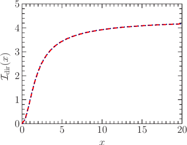
Figure 3: (Color online) The dimensionless integral ${\cal I}_{\rm dir}(x)$ from the instanton vacuum. The numerical result of Eq. (43) is depicted as the red dashed curve whereas that of parametrization given in Eq. (49) is drawn as the blue dotted curve.

One can see almost the one to one correspondence of the numerical calculations and the parametrization Eq. (49).

V.2 Perturbative one-gluon exchange singlet potential in ILM

From Eq. (A.2) it is seen that the perturbative one-gluon exchange potential has the form

$$V_{\rm pert}=g^{2}\left(\frac{\lambda_{a}}{2}\frac{\bar{\lambda}_{b}}{2}\right)\int d\tau\bar{S}_{ab}(\vec{r},\tau).$$ (52)

Using the momentum representation of the averaged gluon propagator in Eq. (16) and the singlet color factor (147) from Appendix A, one can get

$$V_{\rm pert}(r)=-\frac{4}{3}\,g^{2}\int\frac{d^{3}q}{(2\pi)^{3}}\frac{e^{i\vec{q}\cdot\vec{r}}}{q^{2}+M_{g}^{2}(q)}\,.$$ (53)

where $r$ is a distance between $Q$ and $\bar{Q}$ quarks and $M_{g}(q)$ is given by Eq. (18). After the angular integration and introducing the dimensionless variables, $x=r/\rho$ and $y=q\rho$, one can obtain the perturbative one-gluon exchange potential in the form of

$$V_{\rm pert}(r) =-\frac{4\alpha_{s}}{3r}f_{\rm scr}(x),$$ (54)

$$f_{\rm scr}(x) =1-\frac{2x}{\pi}\int_{0}^{\infty}{\rm d}y~{}j_{0}(xy)\frac{3\pi^{2}\lambda{K}_{1}^{2}(y)}{1+3\pi^{2}\lambda{K}_{1}^{2}(y)},$$ (55)

where $f_{\rm scr}(x)$ plays the role of screening function (see Fig. 4).

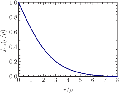
Figure 4: (Color online) Dependence of screening function $f_{\rm scr}$ on $r/\rho$ at ILM parameters $R=1~{}{\rm fm}$ and $\rho=1/3~{}{\rm fm}$.

Naturally, from the the Eq. (55) at the short distances one can obtain the Coulomb-like potential

$$V_{\rm pert}(r) \simeq-\frac{4\alpha_{s}}{3}\left(\frac{1}{r}-A\right)\,,$$ (56)

$$\qquad A =\frac{2}{\pi\rho}\,\int_{0}^{\infty}dy\,\frac{3\pi^{2}\lambda{K}_{1}^{2}(y)}{1+3\pi^{2}\lambda{K}_{1}^{2}(y)}\,.$$ (57)

It is easy to understand the meaning of $A$ comparing with Yukawa-like potential $V_{Y}$ corresponding to the constant gluon mass $M_{Y}$. Its general expression and the behavior at $r\to 0$ are given as

$$V_{Y}(r) =-\frac{4}{3}\,g^{2}\int\frac{d^{3}q}{(2\pi)^{3}}\frac{e^{i\vec{q}\cdot\vec{r}}}{q^{2}+M_{Y}^{2}}$$ (58)

$$=-\frac{4\alpha_{s}}{3r}\exp(-M_{Y}r)$$ (59)

$$\to-\frac{4\alpha_{s}}{3}\left(\frac{1}{r}-M_{Y}\right)+...$$ (60)

In such a way, $M_{Y}=A$ and $M_{Y}$ must be smaller than $M_{g}(0)\simeq 358\,{\rm MeV}$ since the influence of form-factor in $M_{g}(q)$. From Eq. (57) it is seen that $M_{Y}\simeq 218$  MeV at $\rho=1/3$ fm, $R=1$ fm. One can see from the left panel of Fig. 5, that at small $r<0.5\rho$ there is coincidence of $V_{Y}$ in Eq. (60) with the exact numerical result (see Eq. (55)) as it was expected. But at the large distances $r>0.5\rho$ the slope of curve corresponding to the exact solution is different and $V_{Y}$ must be described by another parameter, i.e. $M_{Y,1}\approx 282$ MeV (see the right panel in Fig. 5). This conclusion is natural since the large distance $r$ corresponds to the smaller momentum $q$ and one should have $M_{Y}<M_{Y,1}<M_{g}(0)$.

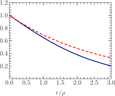
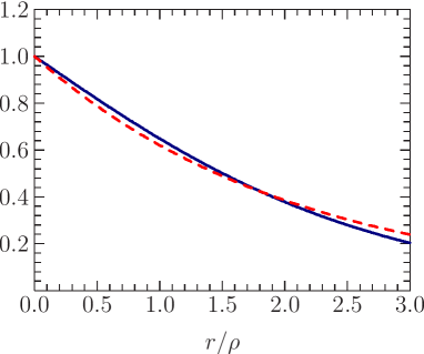
Figure 5: (Color online) Dependence of $\exp(-rM_{Y})$ (left panel) and $\exp(-rM_{Y,1})$ (right panel) on $r/\rho$ (orange color) in comparison with the exact numerical result for $V_{\rm pert}(r/\rho)$ (blue color) at ILM parameters $R=1~{}{\rm fm}$ and $\rho=1/3~{}{\rm fm}$. The effective gluon mass must be different at different regions of $r$ (see the text) and their values in the left and right panels are chosen as $M_{Y}=218$ MeV and $M_{Y,1}=282$ MeV, respectively.

The parametrization of $V_{\rm pert}$ in the form of Yukawa potential may be useful for the quick and crude applications.

For the high accuracy calculations one can parametrize the potential $V_{\rm pert}(r)$ in a much better way. For that purpose we introduce the dimensionless integral ${\cal I}_{\rm pert}(x)$ in the expression of screening function $f_{\rm scr}$ (see Eq. (55)) in such a way

$$f_{\rm scr}(x)=1-\frac{2x}{\pi}\,{\cal I}_{\rm scr}(x).$$ (61)

Then ${\cal I}_{\rm scr}$ can be parametrized with the high precision analogously to ${\cal I}_{\rm dir}$ as

$${\cal I}_{\rm scr}(x) ={\cal I}_{0}^{\rm s}\left\{\sum_{i=1}^{2}\left[a_{i}^{\rm s}x^{2(i-1)}+a_{3}^{\rm s}(-b_{3}^{\rm s}x)^{i}\right]e^{-b_{i}^{\rm s}x^{2}}\right.$$ (62)

$$+\left.\frac{a_{3}^{\rm s}}{x}\left(1-e^{-b_{3}^{\rm s}x^{2}}\right)\right\}.$$ (63)

The parameters corresponding to this parametrization have the values

$${\cal I}^{\rm s}_{0} =0.578695,$$ (64)

$$a_{1}^{\rm s} =1,\quad a_{2}^{\rm s}=0.121348,\quad a_{3}^{\rm s}=2.71619,$$ (65)

$$b_{1}^{\rm s} =0.144123,\quad b_{2}^{\rm s}=0.189758,\quad b_{3}^{\rm s}=b_{1}^{\rm s}$$ (66)

for the ILM parameters $\rho=1/3$ fm and $R=1$  fm. For another set of parameters, $\rho=0.36$ fm and $R=0.89$ fm, one has the following parameters

$${\cal I}^{\rm s}_{0} =0.743964,$$ (67)

$$a_{1}^{\rm s} =1,\quad a_{2}^{\rm s}=-0.0362548,\quad a_{3}^{\rm s}=2.11812,$$ (68)

$$b_{1}^{\rm s} =0.329341,\quad b_{2}^{\rm s}=0.460567,\quad b_{3}^{\rm s}=b_{1}^{\rm s}.$$ (69)

One can see that the relations ${\cal I}_{0}^{\rm s}a_{3}^{\rm s}\simeq\pi/2$ is hold. The comparison of numerical and parametrized forms of ${\cal I}_{\rm scr}(x)$ is shown in Figure 6. Like in the case of ${\cal I}_{\rm dir}$, here also we have almost the one-to-one correspondence.

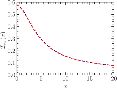
Figure 6: (Color online) The dimensionless integral ${\cal I}_{\rm scr}(x)$ from the instanton vacuum including the perturbative corrections. The numerical result is depicted as the red dashed curve whereas that of parametrization Eq. (63) is drawn as the blue dotted curve. The ILM parameters are set as $\rho=1/3$ fm and $R=1$ fm.

At large distances $r>\rho$ the potential $V_{\rm pert}(r)$ is not long-ranged anymore and quickly goes to zero. In such a way, at large distances the instanton medium produces the screening effect in the one gluon exchange perturbative potential.

VI Order of instanton effects

Obviously, the best and straightforward way of estimation of the instanton effects is the analysis of charmonia and bottmonia states and comparison the results in ILM approach with the results of other phenomenological approaches. For that purpose one needs the spin-dependent parts of the $Q\bar{Q}$ potential. Although the relations between the central and spin-dependent parts of the direct instanton contributions are already known, one should re-calculate such relations in the case of one gluon exchange perturbative interaction which includes the instanton contributions. Such a detailed analysis we will leave for the future work and concentrate here only on the central part of $Q\bar{Q}$ interactions.

In the present work, we will ignore the spin splitting effects in the charmonium spectra and concentrate only on some low lying S-wave states. First, we perform the fully variational calculations considering the different sets of potentials without and with the instanton effects. The next, we consider the instanton effects in the first order pertubation theory and compare with the results of the fully variational calculations. The corresponding conclusions from these studies will be helpful in our future works.

Further, we define the full central $Q\bar{Q}$ potential which includes all possible instanton effects in the following form

$$V(r)=\sigma r+V_{\rm pert}(r)+V_{\rm dir}(r),$$ (70)

which supplies the confinement phenomena at large distances. This potential leads to the standard Cornell’s potential Eq. (1) in the absence of instanton effects. In order to account the instanton effects in the first order perturbation theory we divide the Hamiltonian into two parts

$$H=H_{0}+\tilde{H},$$ (71)

where $H_{0}$ is Hamiltonian of the Cornell’s model and $\tilde{H}$ is the perturbative part of Hamiltonian. They are defined as

$$H_{0} =-\frac{1}{m_{Q}}\vec{\nabla}^{2}+V_{\rm Cornell},$$ (72)

$$\tilde{H} =V-V_{\rm Cornell}\equiv V_{\rm dir}+V_{\rm scr},$$ (73)

$$V_{\rm scr} =-\frac{4\alpha_{s}}{3}(f_{\rm scr}-1).$$ (74)

The results of full variational calculations are presented in Table 1 for the possible two sets of ILM parameters. The details of calculations can be found in Ref. Yakhshiev:2018juj . As an example of the Cornell’s model parameters, we chosed the parameter set MWOI presented in Table I of Ref. Yakhshiev:2018juj . For comparison, in Table 1 we present the results for Cornell’s potential,“Cornell + instanton” potentials which have the nature of instanton contributions from the different regions and also for the full potential which takes into account all possible instanton effects from the different regions.

Table 1: The results of full variational calculations. It is considered only some of the S-wave states corresponding to the charmonium states (Spin dependent parts of interactions are not included). The general parameters are set as $m_{Q}=1275$ MeV and $\sigma=0.17$ GeV². Other ILM and the potential related parameters are given in the table. The first column is radial excitations and the other columns are the results corresponding to the different sets of potentials. All states are given in units of MeV.

		$\rho=1/3$ fm, $R=1$ fm			$\rho=0.36$ fm, $R=0.89$ fm
$n$	$V_{\rm Cornell}$	$V_{\rm Cornell}+V_{\rm scr}$	$V_{\rm Cornell}+V_{\rm dir}$	$V$	$V_{\rm Cornell}+V_{\rm scr}$	$V_{\rm Cornell}+V_{\rm dir}$	$V$
$\alpha_{s}=0.2$
1	3069	3129	3111	3172	3131	3146	3208
2	3611	3664	3682	3736	3661	3747	3798
3	4035	4079	4119	4163	4078	4198	4241
4	4405	4443	4496	4534	4442	4582	4621
$\alpha_{s}=0.4$
1	2905	3026	2943	3063	3031	2973	3100
2	3509	3617	3579	3688	3612	3642	3747
3	3956	4044	4038	4128	4043	4116	4205
4	4337	4414	4428	4505	4413	4514	4591

We note that the both potentials $V_{\rm scr}$ and $V_{\rm dir}$ are positively defined and, therefore, give the positive contributions to the whole spectrum. One can see the corresponding results in the Table 1. Our results are presented for the two values of strong coupling constant, $\alpha_{s}=0.2$ and $\alpha_{s}=0.4$ in order to investigate $\alpha_{s}$ dependence. Obviously, the increasing value of $\alpha_{s}$ leads to the strengthening of Coulomb-like attraction and lowers the states.

The order of instanton contributions is not big but they are not negligible too. One may conclude, that the corresponding instanton effects may be considered as the perturbative corrections. In order to understand this situation better we will consider the first order perturbative corrections to the Cornell’s model results considering the instanton effects as the small perturbations.

The comparisons of the corresponding perturbative and variational calculations are shown in Table 2.

Table 2: The perturbative vs full variational calculations. The first column is radial exitations, 2-4 columns are the first order perturbative corrections, 5-7 columns are the corresponding differences of variational calculations with and without instanton generated potentials, respectively (see explanations in the text). The parameters and other definitions are same as in the Table 1.

	First order perturbative corrections			The corresponding variational calculations
$n$	$V_{\rm scr}$	$V_{\rm dir}$	$V_{\rm scr}+V_{\rm dir}$	“$V_{\rm scr}$”	“$V_{\rm dir}$”	“$V_{\rm scr}+V_{\rm dir}$”
$\alpha_{s}=0.2$, $\rho=1/3$ fm, $R=1$ fm, $\lambda=0.01235$
1	60.124	44.305	104.430	60.119	42.439	102.611
2	52.826	72.224	125.050	52.707	71.438	124.651
3	43.864	84.342	128.206	43.743	83.873	127.954
4	38.247	91.518	129.765	38.172	91.193	129.561
$\alpha_{s}=0.2$, $\rho=0.36$ fm, $R=0.89$ fm, $\lambda=0.02677$
1	61.661	82.116	143.777	61.607	77.142	139.449
2	50.557	138.826	189.383	50.451	136.343	187.599
3	43.144	163.750	206.893	43.047	168.332	205.956
4	37.891	178.749	216.640	37.820	177.813	216.013
$\alpha_{s}=0.4$, $\rho=1/3$ fm, $R=1$ fm, $\lambda=0.01235$
1	120.343	39.088	159.432	120.311	37.369	157.725
2	108.071	70.832	178.902	107.662	69.962	178.584
3	89.237	83.728	172.965	88.733	83.231	172.671
4	77.342	91.216	168.558	77.030	90.877	168.317
$\alpha_{s}=0.4$, $\rho=0.36$ fm, $R=0.89$ fm, , $\lambda=0.02677$
1	125.739	72.026	197.765	125.593	67.620	194.298
2	102.992	135.925	238.918	102.579	133.184	237.412
3	87.474	162.424	249.898	87.085	160.914	249.191
4	76.523	178.078	254.601	76.226	177.090	254.114

In the left-half of the table, we present the first order perturbative corrections due to instantons (see $\tilde{H}$ in Eq. (71)) calculated on a basis of Cornell’s model wave functions corresponding to the Hamiltonian $H_{0}$. On the right-half of the table, we present the corresponding differences of variational calculations with and without instanton generated potentials. For example, “$V_{\rm scr}$” means the difference between the results of the potential models, “$V_{\rm Cornell}+V_{\rm scr}$” and “$V_{\rm Cornell}$”, obtained by means the variational calculations (The corresponding results are presented in Table 1.). It should be compared with the first order perturbative corrections corresponding to the perturbation potential $V_{\rm scr}$. One can see that almost the hundred percent effects due to instantons can be considered as the first order perturbative corrections to the spectrum.

When the value of $\alpha_{s}$ is changed, the general picture will not change if one concentrates to the order of instanton contributions, i.e. they still remain as the first order perturbative corrections. It can be seen from the upper-half and the lower-half parts in Table 2. The relative sizes of all possible instanton effects in comparison with the results corresponding to the Cornell’s model results found to be from 3 % to 6 % depending on the parameters of instanton liquid model and the excitation state, e.g. compare the column $V_{\rm Cornell}$ in Table 1 with the column $V_{\rm scr}+V_{\rm dir}$ in Table 2.

From other side, it is interesting to see that the contribution amount itself increases two times if we concentrate on $V_{\rm scr}$ value (compare the upper-half and the lower-half parts of Table  2). This is obvious result while the parameter $\alpha_{s}$ is overall factor in the expression of $V_{\rm scr}$ in Eq. (54). In contrast, $V_{\rm dir}$ is independent on parameter $\alpha_{s}$ and depends on it only by the wave function changes which are small (again compare the upper-half and the lower-half parts of Table  2).

It is also interesting to note, that the increasing value of packing parameter $\lambda$ will not change much the contribution from screening part $V_{\rm scr}$. This can be seen by comparisons of $V_{\rm scr}$ or “$V_{\rm scr}$” values for the fixed value of $\alpha_{s}$ (see the upper-half or the lower-half part of Table  2). This is due to the fact that $f_{\rm scr}$ depends on $\lambda$ in a nontrivial way (see Eq. (55)). In contrast, the contribution from the direct instanton interactions increases almost linearly which is seen from the columns $V_{\rm dir}$ or “$V_{\rm dir}$” in Table 2. One can note, that an approximately two times increased value of $\lambda$ increases the value of direct instanton interaction contributions also approximately two times (again see the upper-half or the lower-half part of Table 2). This can be seen also from the expression of $V_{\rm dir}$ where $\lambda$ is overall factor (see Eq. (39)).

Although the direct comparisons of results with the experimental data can be done after inclusions of the spin-dependent parts in the potential, here we already can make some qualitative predictions. For that purpose, first we will refer to the Tables  I and  II presented in Ref. Yakhshiev:2018juj . One can see, that with the value of $\alpha_{s}=0.2068$ denoted as MWOI it is possible to fit the experimental data by using Cornell’s type potential and concentrating on the first six low-lying S-wave states during the fitting process (see Table II in Ref. Yakhshiev:2018juj and explanations there). While the low-lying states are reproduced more or less well the excited states are lower estimated. Inclusion of the direct instanton interactions improves much better the low-lying states but the excited states are overestimated (see columns M-I and M-IIb in Table II of Ref. Yakhshiev:2018juj ).

Now, let us concentrate back to the Table 2 in present work. From the column $V_{\rm dir}$ or “$V_{\rm dir}$” on can see that the direct instanton interactions will contribute more and more to the excited stated. It is remarkable, that the inclusion of screening effect from the instantons changes the situation drastically. This is due to the fact that the screening effect softens the contributions to excited states from the instantons (see columns $V_{\rm scr}$ or “$V_{\rm scr}$”). As a result, the instanton effects from both $V_{\rm scr}$ and $V_{\rm dir}$ accumulated in such a way that the ground state is changed in a different way while the excited states have more or less overall shift effect (see columns $V_{\rm scr}+V_{\rm dir}$ or “$V_{\rm scr}+V_{\rm dir}$”). This situation may be quite helpful in describing the experimental data related to the charmonium states by using the potential approach in the framework of instanton liquid model.

Summarizing all our discussions we note, that the instanton effects are at the level of few percents. Nevertheless, one cannot ignore the instanton effects in the heavy quarkonium spectra. They may also be important during the fine tuning processes of the whole spectrum which takes into account the spin-spin, spin-orbit and tensor interactions.

VII Summary and Outlook

In this work we studied one body and two body correllators corresponding to the heavy quark sector in the framework of Instanton Liquid Model by inclusion also the perturbative corrections. Although the instantons cannot explain a confinement mechanism, we have shown that they play a nontrivial role not only in the nonperturbative region $r\sim\rho$ but also in the perturbative region $r<\rho$. In the perturbative region the instantons will affect in such way that the one gluon exchange perturbative potential becomes the short range and remains the screened at large distances. In such a way, at short distances the OGE potential including the instanton effects can be approximated by a Yukawa-type potential with the corresponding dynamical gluon mass playing the role of parameter in the exponent. The direct instanton effects reproduce an overall shift at the nonperturbative region which can be accounted as the renormalization of heavy quark mass in the instanton medium. Consequently, our conclusion is that the instanton effects in both, perturbative and nonperturbative, regions are important for understanding the heavy quark physics.

At quantative level, we also estimated the instanton effects to the whole spectrum and found out that they can completely be considered as the first order perturbative corrections. The relative size of instanton effects in the spectra of heavy quarkonia at the level of few percents and should be taken into account during the fine tuning processes. In Ref. Yakhshiev:2018juj it was discussed that the direct instanton effects from the nonperturbative region may explain the origin of phenomenological potential parameters fitted to the spectrum of heavy quarkonia. The inclusion of instanton effects in the perturbative region may help not only in the qualitative understanding $Q\bar{Q}$ interactions but also at the quantitave level concerned on more accurate description of spectra. For that purpose, one should take into account the changes in the spin-dependent potentials due to instanton effects in the perturbative region. This can be done by means of relating the central and spin-dependent potential in the framework of heavy quark effective theory. The corresponding studies are currently under the way.

Appendix A Detailed calculation of correlators

In this appendix we discuss the details of perturbative expansions for the quark and $Q\bar{Q}$ correlators, and the corresponding ILM contributions to the heavy quark mass and $Q\bar{Q}$ potential.

A.1 Contribution to the heavy quark mass in ILM

We begin with the expansion of the propagator in Eq. (19). First we note, that the non-averaged in the instanton medium heavy quark propagator in operator notations $D=\theta^{-1}-gA(\xi)$ is given by the expansion

$$\left.\exp\left[\frac{1}{2}\left(\frac{\delta}{\delta a}S\frac{\delta}{\delta a}\right)\right]\frac{1}{D-ga}\right|_{a=0}$$ (75)

$$~{}=\sum_{m=0}^{\infty}\frac{1}{m!}\left[\frac{1}{2}\left(\frac{\delta}{\delta a}S\frac{\delta}{\delta a}\right)\right]^{m}\left(\frac{1}{D}ga\right)^{2m}\frac{1}{D}$$

$$~{}=\sum_{m=0}^{\infty}\left(g^{2}\frac{1}{D}\left(S\frac{1}{D}\right)\right)^{m}\frac{1}{D}.$$ (76)

It is easy to find that the lowest order ${\cal{O}}(\alpha_{s})$ peturbative correction to the heavy quark propagator is

$$\frac{1}{D}\left(\frac{\delta}{\delta a}S\frac{\delta}{\delta a}\right)\left(ag\frac{1}{D}\right)^{2}$$ (77)

$$~{}\rightarrow g^{2}\langle x_{0}|\frac{1}{D}|x_{1}\rangle(S_{ab}(x_{1},x_{2})+S_{ba}(x_{2},x_{1}))$$ (78)

$$~{}\times\frac{\lambda_{a}}{2}\langle x_{1}|\frac{1}{D}|x_{2}\rangle\frac{\lambda_{b}}{2}\langle x_{2}|\frac{1}{D}|x_{3}\rangle$$ (79)

$$~{}\equiv g^{2}\langle x_{0}|\frac{1}{D}|x_{1}\rangle\langle x_{1}|(S\frac{1}{D})|x_{2}\rangle\langle x_{2}|\frac{1}{D}|x_{3}\rangle,$$ (80)

where repeating $x_{i}$ means integration over $x_{i}$. Also, $g^{2}(S\frac{1}{D})$ has a meaning of the perturbative heavy quark mass operator $\Sigma$ in the lowest order $O(\alpha_{s})$ and was defined by its matrix element

$$\langle x_{1}|\Sigma|x_{2}\rangle = g^{2}\langle x_{1}|(S\frac{1}{D})|x_{2}\rangle$$ (81)

$$\equiv g^{2}(S_{ab}(x_{1},x_{2})+S_{ba}(x_{2},x_{1}))$$ (82)

$$\times \frac{\lambda_{a}}{2}\langle x_{1}|\frac{1}{D}|x_{2}\rangle\frac{\lambda_{b}}{2}.$$ (83)

Analogously, the next order contribution ${\cal{O}}(\alpha_{s}^{2})$ has form

$$\frac{1}{D}\left(\frac{\delta}{\delta a}S\frac{\delta}{\delta a}\right)^{2}\left(ag\frac{1}{D}\right)^{4}$$ (84)

$$~{}\rightarrow g^{4}\langle x_{0}|\frac{1}{D}|x_{1}\rangle\left(\frac{\delta}{\delta a(y)}S(y,z)\frac{\delta}{\delta a(z)}\right)$$ (85)

$$~{}\times\left(\frac{\delta}{\delta a(y^{\prime})}S(y^{\prime},z^{\prime})\frac{\delta}{\delta a(z^{\prime})}\right)$$ (86)

$$~{}\times\left(a(x_{1})\langle x_{1}|\frac{1}{D}|x_{2}\rangle a(x_{2})\langle x_{2}|\frac{1}{D}|x_{3}\rangle\right)$$ (87)

$$~{}\times\left(a(x_{3})\langle x_{3}|\frac{1}{D}|x_{4}\rangle a(x_{4})\langle x_{4}|\frac{1}{D}|x_{5}\rangle\right)$$ (88)

$$~{}\times\langle x_{0}|\frac{1}{D}|x_{1}\rangle\langle x_{1}|S(x_{1},x_{2})+S(x_{2},x_{1})|x_{2}\rangle$$ (89)

$$~{}\times\langle x_{2}|\frac{1}{D}|x_{3}\rangle\langle x_{3}|S(x_{3},x_{4})+S(x_{4},x_{3})|x_{4}\rangle$$ (90)

$$~{}\times\langle x_{4}|\frac{1}{D}|x_{5}\rangle+[(x_{i_{1}},x_{i_{2}})\to(x_{j_{1}},x_{j_{2}})].$$

We define the sum of all irreducible diagrams as $\Sigma$, which has the following form in diagram representation

$$\Sigma$$ =++… (91)

Now, the series (76) can be summed up according to the geometrical progression

$$\frac{1}{D}\left(1+\Sigma\frac{1}{D}+\Sigma\frac{1}{D}\Sigma\frac{1}{D}+\cdots\right) = \frac{1}{D}\frac{1}{1-\Sigma\frac{1}{D}}$$ (92)

$$= \frac{1}{D-\Sigma}.$$ (93)

However, as we already mentioned in the text, we neglected by the gluon self-interaction terms ${\cal{O}}(g^{3},g^{4})$. Therefore, we have to take into account the heavy quark mass operator only in the lowest order ${\cal{O}}(\alpha_{s})$ single-loop approximation. That is $\Sigma=g^{2}(SD^{-1})$ defined by Eq. (83).

Consequently, we obtain the following expression for the non-averaged heavy quark propagator

$$\frac{1}{D-g^{2}(SD^{-1})}.$$ (94)

Further we averaging Eq. (94) over the instanton ensemble in ${\cal{O}}(\lambda,\alpha_{s}\lambda^{1/2})$ approximation, which leads to further simplification of the perturbative mass operator as $g^{2}(SD^{-1})\approx g^{2}(S\theta)$.

It is obvious, that in order to have the ILM perturbative heavy quark mass operator we have to remove from $\Sigma$ the perturbative heavy quark mass operator in the empty space as $\Sigma-\Sigma_{0}$, where $\Sigma_{0}=g^{2}(S^{0}\theta)+O(g^{4}).$ Then, Eq. (94), should be rewritten as

$$\left[\theta^{-1}-g\sum_{i}A_{i}(\xi_{i})-g^{2}\left(\sum_{j}\Delta S^{j}(\xi_{j})\theta\right)\right]^{-1}.\quad$$ (95)

To calculate ILM direct and ILM perturbative mass contributions we use more definitive form of Pobylitsa Eq. (24) as

$$\langle t_{2}|w^{-1}|t_{1}\rangle=-\delta^{{}^{\prime}}(t_{2}-t_{1})$$ (96)

$$~{}+\sum_{\pm}\int dz_{4,\pm}f(t_{2}-z_{4,\pm},t_{1}-z_{4,\pm})$$ (97)

$$~{}+g(t_{2},t_{1}),$$ (98)

where

$$f(t_{2}-z_{4,\pm},t_{1}-z_{4,\pm})$$ (99)

$$~{}=-\frac{N}{2V}\sum_{\pm}{\rm tr}_{c}\int d^{3}z_{\pm}\,\langle t_{2}|\theta^{-1}(w_{\pm}-\theta)\theta^{-1}|t_{1}\rangle$$ (100)

$$g(t_{2},t_{1})=-g^{2}\langle t_{2}|\left((\bar{S}-S^{0})\theta\right)|t_{1}\rangle.$$ (101)

In the last equations $w_{\pm}\equiv(\theta^{-1}-A_{\pm}(\xi_{\pm}))^{-1}$ and ‘$\pm$’ indexes correspond to the instanton/antiinstanton, respectively. Introducing the Fourier transformation Diakonov:1989un

$$\langle t_{2}|w|t_{1}\rangle = \int\frac{d\omega}{2\pi}\exp[i\omega(t_{2}-t_{1})]w(\omega)$$ (102)

$$= \int\frac{d\omega}{2\pi}\exp[i\omega(t_{2}-t_{1})]\frac{1}{w^{-1}(\omega)}$$ (103)

and using Pobylitsa Eq. (98) one can find that

$$\langle t_{2}|w|t_{1}\rangle = \int\frac{d\omega}{2\pi}\exp[i\omega(t_{2}-t_{1})]\frac{1}{i\omega+f(\omega)+g(\omega)}$$

$$f_{\pm}(\omega) = \int dt_{2}\,dt_{1}\exp[-i\omega t_{2}+i\omega t_{1}]$$ (104)

$$\times f(t_{2}-z_{4,\pm},t_{1}-z_{4,\pm})_{|_{z_{4,\pm}=0}}$$ (105)

$$g(\omega) = \int d\tau\exp[i\omega\tau]g(\tau),~{}\tau=t_{2}-t_{1}.$$ (106)

One can see, that there is a pole within the approximations discussed above

$$i\omega_{0}+f(0)+g(0)=0.$$

According to this pole we obtain ILM direct and ILM perturbative contributions to the heavy quark mass from the time dependence of the heavy quark propagator Eq. (106) as

$$\langle t_{2}|w|t_{1}\rangle \sim \exp(-\Delta M_{Q}(t_{2}-t_{1})),$$ (107)

$$\Delta M_{Q} = \Delta M_{Q}^{\rm dir}+\Delta M_{Q}^{\rm pert},\,\,\,$$

$$\Delta M_{Q}^{\rm dir} = f(0),$$ (108)

$$\Delta M_{Q}^{\rm pert} = g(0).$$ (109)

Note, that the direct instanton contributions to the heavy quark mass $\Delta M_{Q}^{\rm dir}$ was calculated in Ref. Diakonov:1989un .

Taking into account the color factor in $((\bar{S}-S^{0})\theta)$, which is $\frac{\lambda_{a}}{2}\frac{\lambda_{b}}{2}\delta_{ab}=\frac{4}{N_{c}}I$ ($I$ is $N_{c}\times N_{c}$ unit matrix) we have ILM perturbative heavy quark mass contribution in the following form

$$\Delta M_{Q}^{\rm pert}I = -g^{2}\int_{-\infty}^{\infty}d(t_{2}-t_{1})\langle t_{2}|\left((\bar{S}-S^{0})\theta\right)|t_{1}\rangle$$ (110)

$$= -g^{2}\frac{\lambda_{a}}{2}\frac{\lambda_{b}}{2}\int_{0}^{\infty}dt(\bar{S}_{ab}(t)-S_{ab}^{0}(t))$$ (111)

$$= \frac{2}{N_{c}}I\,g^{2}\int\frac{d^{3}k}{(2\pi)^{3}}\frac{M_{g}^{2}(k)}{k^{2}\left[k^{2}+M_{g}^{2}(k)\right]}$$

$$\leq \frac{2}{N_{c}}I\alpha_{s}M_{g}(0).$$

One can estimate, that

$$\Delta M_{Q}^{\rm pert} \leq \frac{2}{N_{c}}\alpha_{s}M_{g}(0)\sim M_{Q}^{\rm dir}\sim 70\,{\rm MeV}$$ (113)

at the values of parameters $N_{c}=3$, $\alpha_{s}=0.3,\,\rho=1/3\,{\rm fm}$, $R=1\,{\rm fm}.$

A.2 Perturbative contribution to the heavy quark - antiquark potential in ILM

We will proceed with the $Q\bar{Q}$ correlator Eq. (32) in an analogous way what we did with the heavy quark propagator.

Consequently, for the non-averaged $Q\bar{Q}$ correlator Eq. (32) one can write the expansion

$$\exp\left[\frac{1}{2}\sum_{i\neq j=1}^{2}\left(\frac{\delta}{\delta a^{(i)}}S^{(ij)}(\xi)\frac{\delta}{\delta a^{(j)}}\right)\right]$$ (114)

$$~{}\times\left.\frac{1}{D^{(1)}-ga^{(1)}}\frac{1}{\bar{D}^{(2)}-g\bar{a}^{(2)}}\right|_{a=0}$$ (115)

$$~{}=\sum_{m=0}^{\infty}\frac{1}{m!}\left(\frac{g^{2}}{2}\right)^{m}\left[\sum_{i\neq j=1}^{2}\left(\frac{\delta}{\delta a^{(i)}}S^{(ij)}(\xi)\frac{\delta}{\delta a^{(j)}}\right)\right]^{m}$$ (116)

$$~{}\times\left(\frac{1}{D^{(1)}}a^{(1)}\right)^{m}\frac{1}{D^{(1)}}\left(\frac{1}{\bar{D}^{(2)}}\bar{a}^{(2)}\right)^{m}\frac{1}{\bar{D}^{(2)}}.$$ (117)

For the lowest order ${\cal{O}}(\alpha_{s})$ term we obtain the explicit expression

$$\frac{g^{2}}{2}\int dx_{2}^{(1)}dx_{2}^{(2)}$$ (118)

$$\times\langle x^{(1)}_{3}|\frac{1}{D^{(1)}}|x_{2}^{(1)}\rangle\frac{\lambda_{a}}{2}S_{ab}^{(12)}(x^{(1)}_{2},x^{(2)}_{2})\langle x_{2}^{(1)}|\frac{1}{D^{(1)}}|x^{(1)}_{1}\rangle$$ (119)

$$\times\langle x^{(2)}_{1}|\frac{1}{\bar{D}^{(2)}}|x_{2}^{(2)}\rangle\frac{\bar{\lambda}_{b}}{2}\langle x_{2}^{(2)}|\frac{1}{\bar{D}^{(2)}}|x^{(2)}_{3}\rangle$$ (120)

$$+\langle x^{(1)}_{3}|\frac{1}{D^{(1)}}|x_{2}^{(1)}\rangle\frac{\lambda_{b}}{2}S_{ba}^{(21)}(x^{(2)}_{2},x^{(1)}_{2})\langle x_{2}^{(1)}|\frac{1}{D^{(1)}}|x^{(1)}_{1}\rangle$$ (121)

$$\times\langle x^{(2)}_{1}|\frac{1}{\bar{D}^{(2)}}|x_{2}^{(2)}\rangle\frac{\bar{\lambda}_{a}}{2}\langle x_{2}^{(2)}|\frac{1}{\bar{D}^{(2)}}|x^{(2)}_{3}\rangle.$$ (122)

Accordingly, the lowest ${\cal O}(\alpha_{s}\lambda^{1/2})$ contribution to $W$ is given by

$$g^{2}\int dx_{2}^{(1)}dx_{2}^{(2)}\langle x^{(1)}_{3}|\theta^{(1)}|x_{2}^{(1)}\rangle\langle x_{2}^{(1)}|\theta^{(1)}|x^{(1)}_{1}\rangle$$ (123)

$$~{}\times\frac{\lambda_{a}}{2}\frac{\bar{\lambda}_{b}}{2}\bar{S}_{ab}(x^{(1)}_{2}-x^{(2)}_{2})$$ (124)

$$~{}\times\langle x^{(2)}_{1}|\theta^{(2)}|x_{2}^{(2)}\rangle\langle x_{2}^{(2)}|\theta^{(2)}|x^{(2)}_{3}\rangle,$$ (125)

which correspond to the first diagram in the following series of irreducible diagrams (126)

++… (126)

In the approximation ${\cal{O}}(\alpha_{s}\lambda^{1/2})$, one should sum up according to the geometrical progression and make a ladder by repetition of only the first diagram in (126). We expect that this diagram will provide the perturbative contribution to the $Q\bar{Q}$ potential in the approximation ${\cal{O}}(\alpha_{s}\lambda^{1/2})$. The corresponding matrix element is given by

$$g^{2}\frac{\lambda_{a}}{2}\frac{\bar{\lambda}_{b}}{2}\int_{t_{1}}^{t_{3}}\int_{t_{1}}^{t_{3}}dt_{2}^{(1)}dt_{2}^{(2)}\bar{S}_{ab}(\vec{r},t^{(1)}_{2}-t^{(2)}_{2})$$ (127)

$$~{}=(t_{3}-t_{1})g^{2}\frac{\lambda_{a}}{2}\frac{\bar{\lambda}_{a}}{2}\int\!\!\frac{d^{3}k}{(2\pi)^{3}}\frac{e^{i\vec{k}\vec{r}}}{\vec{k}^{2}+M_{g}^{2}(\vec{k})}.\qquad$$ (128)

In the operator form one has

$$W = \int D\xi\frac{1}{D^{(1)}}\frac{1}{D^{(2)}}+g^{2}\theta^{(1)}\theta^{(2)}$$ (130)

$$\times\frac{\lambda_{a}}{2}\frac{\bar{\lambda}_{b}}{2}\bar{S}_{ab}\theta^{(1)}\theta^{(2)}\,+...$$

$$\bar{S}_{ab} = \int D\xi\,S_{ab}^{(12)}.$$

Here the matrix element of operator $S^{(12)}$ is given by

$$\langle x^{(1)}_{2},x^{(2)}_{2}|S^{(12)}|x^{(1)}_{1},x^{(2)}_{1}\rangle$$ (131)

$$~{}=S^{(12)}(x^{(2)}_{1},x^{(1)}_{1})\delta^{4}(x^{(2)}_{2}-x^{(2)}_{1})$$ (132)

$$~{}\times\delta^{4}(x^{(1)}_{2}-x^{(1)}_{1}).$$ (133)

One has the similar expression for $S^{(21)}$, while

$$\langle x^{(1)}_{2},x^{(2)}_{2}|\bar{S}|x^{(1)}_{1},x^{(2)}_{1}\rangle$$ (134)

$$~{}=\bar{S}(x^{(2)}_{1}-x^{(1)}_{1})\delta^{4}(x^{(2)}_{2}-x^{(2)}_{1})$$ (135)

$$~{}\times\delta^{4}(x^{(1)}_{2}-x^{(1)}_{1}).$$ (136)

Operators $S^{(12)}$ and $S^{(21)}$ do not commute with $D^{(1)}$ and $D^{(2)}$ operators since they are acting in both subspaces. Formal expression for the operator $W$ is given by Eq. (35) and Pobylitsa equation in the approximation ${\cal O}(\lambda,\alpha_{s}\lambda^{1/2})$ is given by Eq. (38), where we will use

$$\int D\xi\,S_{ab}^{(12)}(x^{(1)}_{2},x^{(2)}_{2})=\bar{S}_{ab}(x^{(1)}_{2}-x^{(2)}_{2}).$$

Asymptotically the $Q\bar{Q}$ correlator at large time $T\to\infty$ is given by $\exp(-VT)$ and can be calculated in accordance with the approach used in the Eqs. (103)-(109) Diakonov:1989un . Consequently, the $Q\bar{Q}$ potential also can be written as

$$V=V_{\rm dir}+V_{\rm pert}.$$

As it is shown in Ref. Diakonov:1989un the direct instanton induced $Q\bar{Q}$ potential $V_{\rm dir}$ is originated from the matrix elements of the first and second terms in the Eq. (38). It is explicitly expressed as

$$V_{\rm dir}=-\int dt^{(1)}_{2}\,dt^{(2)}_{2}\,dt^{(1)}_{1}\,dt^{(2)}_{1}\sum_{i}\int d\xi_{i}\langle x^{(1)}_{2}\,x^{(2)}_{2}|$$ (137)

$$~{}\times\theta^{(1)-1}\theta^{(2)-1}\left(\frac{1}{D_{i}^{(1)}}\frac{1}{D_{i}^{(2)}}-\theta^{(1)}\theta^{(2)}\right)$$ (138)

$$~{}\times\theta^{(1)-1}\theta^{(2)-1}|x^{(1)}_{1}\,x^{(2)}_{1}\rangle.$$ (139)

For the one-gluon exchange $Q\bar{Q}$ potential in ILM $V_{\rm pert}$ we have the similar relation

$$V_{\rm pert} = \int dt^{(1)}_{2}\,dt^{(2)}_{2}\,dt^{(1)}_{1}\,dt^{(2)}_{1}\frac{\lambda_{a}}{2}\frac{\bar{\lambda}_{b}}{2}$$

$$~{}\times\left(S^{0}_{ab}+\sum_{i}\int d\xi_{i}\Delta S_{ab}\right)(\vec{r},t^{(1)}_{1},t^{(2)}_{1})$$

$$~{}\times\delta(t^{(1)}_{1}-t^{(1)}_{2})\delta(t^{(2)}_{1}-t^{(2)}_{2})$$

$$~{}=g^{2}\frac{\lambda_{a}}{2}\frac{\bar{\lambda}_{b}}{2}\int d\tau\bar{S}_{ab}(r,\tau),$$

$$\tau=t^{(1)}_{1}-t^{(2)}_{1}.$$

For the color factor in Eq. (A.2) we have the following expressions (see brown1979 )

$$\frac{\lambda_{a}}{2}\frac{\lambda_{a}}{2}=\frac{\bar{\lambda}_{a}}{2}\frac{\bar{\lambda}_{a}}{2}=\frac{N_{c}^{2}-1}{2N_{c}}I,\,\,\,\bar{\lambda}_{a}=-\lambda_{a}^{T},$$ (144)

$$I_{a}=\frac{\lambda_{a}}{2}+\frac{\bar{\lambda}_{a}}{2},\,\,\,I_{a}I_{a}=\frac{N_{c}^{2}-1}{N_{c}}I+2\frac{\lambda_{a}}{2}\frac{\bar{\lambda}_{a}}{2}.$$ (145)

One has $(I_{a}I_{a})_{S}=0$ in the color singlet state and $(I_{a}I_{a})_{A}=N_{c}$ in the adjoint state, respectively. Finally, one has

$$\left(\frac{\lambda_{a}}{2}\frac{\bar{\lambda}_{a}}{2}\right)_{S} = -\frac{N_{c}^{2}-1}{2N_{c}}I,$$ (146)

$$\left(\frac{\lambda_{a}}{2}\frac{\bar{\lambda}_{a}}{2}\right)_{A} = \frac{1}{2N_{c}}I.$$ (147)

References

- (1) E. Eichten, K. Gottfried, T. Kinoshita, J. B. Kogut, K. D. Lane and T. M. Yan, “The Spectrum of Charmonium”, Phys. Rev. Lett. 34, 369 (1975) Erratum: [Phys. Rev. Lett. 36, 1276 (1976)].
- (2) G. S. Bali, “QCD forces and heavy quark bound states”, Phys. Rept. 343, 1 (2001).
- (3) N. Brambilla, A. Vairo, X. Garcia Tormo, i and J. Soto, “The QCD static energy at NNNLL”, Phys. Rev. D 80 (2009), 034016.
- (4) V. Mateu, P. G. Ortega, D. R. Entem and F. Fernández, “Calibrating the Naïve Cornell Model with NRQCD”, Eur. Phys. J. C 79 (2019) 323.
- (5) D. Diakonov, “Instantons at work”, Prog. Part. Nucl. Phys. 51 (2003) 173.
- (6) T. Schafer and E. V. Shuryak, “Instantons in QCD”, Rev. Mod. Phys. 70 (1998) 323.
- (7) Edward Shuryak, “Lectures on nonperturbative QCD ( Nonperturbative Topological Phenomena in QCD and Related Theories)”, [arXiv:1812.01509 [hep-ph]].
- (8) K. Goeke, M. M. Musakhanov and M. Siddikov, “Low energy constants of chi PT from the instanton vacuum model”, Phys. Rev. D 76 (2007) 076007.
- (9) K. Goeke, H. C. Kim, M. M. Musakhanov and M. Siddikov, “1/N(c) corrections to the magnetic susceptibility of the QCD vacuum”, Phys. Rev. D 76 (2007) 116007.
- (10) K. Goeke, M. Musakhanov and M. Siddikov, “QCD isospin breaking ChPT low-energy constants from the instanton vacuum”, Phys. Rev. D 81 (2010) 054029.
- (11) M. Musakhanov, “QCD in Infrared Region and Spontaneous Breaking of the Chiral Symmetry”, PoS Baldin-ISHEPP-XXI (2012) 008.
- (12) M. Musakhanov, “Gluons, Heavy and Light Quarks in the QCD Vacuum”, EPJ Web Conf. 182 (2018) 02092.
- (13) L.D. Faddeev, “Looking for multi-dimensional solitons” in: Non-local Field Theories, Dubna, 1976.
- (14) R. Jackiw and C. Rebbi, “Vacuum Periodicity in a Yang-Mills Quantum Theory”, Phys. Rev. Lett. 37 (1976) 172.
- (15) A. Belavin, A. M. Polyakov, A. Schwartz and Y. Tyupkin, “Pseudoparticle Solutions of the Yang-Mills Equations”, Phys. Lett. B 59 (1975) 85.
- (16) M. Chu, J. Grandy, S. Huang and J. W. Negele, “Evidence for the role of instantons in hadron structure from lattice QCD”, Phys. Rev. D 49 (1994) 6039.
- (17) J. W. Negele, “Instantons, the QCD vacuum, and hadronic physics”, Nucl. Phys. B Proc. Suppl. 73 (1999) 92.
- (18) T. A. DeGrand, “Short distance current correlators: Comparing lattice simulations to the instanton liquid”, Phys. Rev. D 64 (2001) 094508.
- (19) P. Faccioli and T. A. DeGrand, “Evidence for instanton induced dynamics, from lattice QCD,” Phys. Rev. Lett. 91 (2003) 182001.
- (20) R. Millo and P. Faccioli, “Computing the Effective Hamiltonian of Low-Energy Vacuum Gauge Fields”, Phys. Rev. D 84 (2011) 034504.
- (21) T. C. Kraan and P. van Baal, “Exact T duality between calorons and Taub - NUT spaces”, Phys. Lett. B 428 (1998) 268.
- (22) T. C. Kraan and P. van Baal, “Periodic instantons with nontrivial holonomy”, Nucl. Phys. B 533 (1998) 627.
- (23) K. M. Lee and C. h. Lu, “SU(2) calorons and magnetic monopoles”, Phys. Rev. D 58 (1998) 025011.
- (24) D. Diakonov, “Topology and confinement”, Nucl. Phys. B Proc. Suppl. 195 (2009) 5.
- (25) Y. Liu, E. Shuryak and I. Zahed, “Confining dyon-antidyon Coulomb liquid model. I.”, Phys. Rev. D 92 (2015) 085006.
- (26) Y. Liu, E. Shuryak and I. Zahed, “Light quarks in the screened dyon-antidyon Coulomb liquid model. II.”, Phys. Rev. D 92 (2015) 085007.
- (27) S. Digal, O. Kaczmarek, F. Karsch and H. Satz, “Heavy quark interactions in finite temperature QCD”, Eur. Phys. J. C 43 (2005) 71.
- (28) E. Eichten, K. Gottfried, T. Kinoshita, K. Lane and T. M. Yan, “Charmonium: Comparison with Experiment”, Phys. Rev. D 21 (1980) 203.
- (29) Y. He, F. Wang and C. W. Wong, “Nucleon Core Size and Nuclear Forces”, Phys. Lett. B 168 (1986) 177.
- (30) W. Weise, “Quarks, chiral symmetry and dynamics of nuclear constituents”, in:Quarks and Nuclei, World Scientific, 1985.
- (31) R.Tegen, “Nucleon form factors from elastic scattering of polarized leptons (, , ) from polarized nucleons” in:Weak and Electromagnetic Interactions in Nuclei, Springer, 1986.
- (32) D. Diakonov, V. Petrov and P. Pobylitsa, “The Wilson Loop and Heavy Quark Potential in the Instanton Vacuum”, Phys. Lett. B 226 (1989) 372.
- (33) L. S. Brown and W. I. Weisberger, “Remarks on the Static Potential in Quantum Chromodynamics”, Phys. Rev. D 20 (1979) 3239.
- (34) P. Pobylitsa, “The Quark Propagator and Correlation Functions in the Instanton Vacuum”, Phys. Lett. B 226 (1989) 387.
- (35) M. Musakhanov and O. Egamberdiev, “Dynamical gluon mass in the instanton vacuum model”, Phys. Lett. B 779 (2018) 206.
- (36) T. Schafer and E. V. Shuryak, “Glueballs and instantons”, Phys. Rev. Lett. 75 (1995) 1707.
- (37) M. C. Tichy and P. Faccioli, “The Scalar glueball in the instanton vacuum”, Eur. Phys. J. C 63 (2009) 423.
- (38) P. de Forcrand and K. F. Liu, “Glueball wave functions in lattice gauge calculations”, Phys. Rev. Lett. 69 (1992) 245.
- (39) D. Weingarten, “QCD spectroscopy”, Nucl. Phys. B Proc. Suppl. 34 (1994) 29.
- (40) H. Chen, J. Sexton, A. Vaccarino and D. Weingarten, “The Scalar and tensor glueballs in the valence approximation”, Nucl. Phys. B Proc. Suppl. 34 (1994) 357.
- (41) C. J. Morningstar and M. J. Peardon, “The Glueball spectrum from an anisotropic lattice study”, Phys. Rev. D 60 (1999) 034509.
- (42) A. Athenodorou and M. Teper, “The glueball spectrum of SU(3) gauge theory in 3+1 dimension”, [arXiv:2007.06422 [hep-lat]].
- (43) H. B. Meyer and M. J. Teper, “Glueball Regge trajectories and the pomeron: A Lattice study”, Phys. Lett. B 605 (2005) 344.
- (44) H. B. Meyer, “Glueball regge trajectories”, [arXiv:hep-lat/0508002 [hep-lat]].
- (45) U. T. Yakhshiev, H. C. Kim, M. M. Musakhanov, E. Hiyama and B. Turimov, “Instanton effects on the heavy-quark static potential”, Chin. Phys. C 41 (2017) 083102.
- (46) U. T. Yakhshiev, H. C. Kim and E. Hiyama, “Instanton effects on charmonium states”, Phys. Rev. D 98 (2018) 114036.