A Bayesian Approach to Modelling Multi-Messenger Emission from Blazars using Lepto-Hadronic Kinetic Equations

Abstract

Blazar TXS 0506+056 is the main candidate for a coincident neutrino and gamma-ray flare event. In this paper, we present a detailed kinetic lepto-hadronic emission model capable of producing a photon and neutrino spectrum given a set of parameters. Our model includes a range of large-scale geometries and both dynamical and steady-state injection models for electrons and protons. We link this model with a Markov Chain Monte Carlo sampler to obtain a powerful statistical tool that allows us to both fit the Spectral Energy Distribution and study the probability density functions and correlations of the parameters. Assuming a fiducial neutrino flux, we demonstrate how multi-messenger observations can be modelled jointly in a Bayesian framework. We find the best parameters for each of the variants of the model tested and report on their cross-correlations. Additionally, we confirm that reproducing the neutrino flux of TXS 0506+056 requires an extreme proton to electron ratio either in the local acceleration process or from external injection.

1 Introduction

The modelling of blazar emission and blazar flares is a topic with a long history (see for example Böttcher, 2019), yet a number of questions still remain open. Firstly, the nature of the hot emitting plasma remains debated. Early models were mostly leptonic (Jones, 1968), in the sense that only electrons and positrons were considered to play a role in the emission. More recently, lepto-hadronic and hadronic models have started to gain a wide acceptance (see e.g. (Mastichiadis & Kirk, 1995; Mastichiadis et al., 2005; Cerruti et al., 2015; Petropoulou & Mastichiadis, 2015; Gao et al., 2017)). Secondly, the number of relevant emitting plasma zones remains unknown. Currently, the main models are based on the assumptions of a single emission zone (a spherical blob) (Böttcher et al., 2013; Cerruti et al., 2018; Keivani et al., 2018) or two main emission zones (jet and sheath models) (MacDonald et al., 2015; Potter, 2018), although some multi zone emission models exist (Graff et al., 2008; Böttcher & Dermer, 2010). Thirdly, the plasma heating mechanisms remain poorly understood. Proposed mechanisms include Magnetic Reconnection (Morris et al., 2019; Petropoulou et al., 2019) and Internal Shocks (Spada et al., 2001; Kino et al., 2004; Böttcher & Dermer, 2010; Pe’er et al., 2017).

Recently, a mayor milestone was achieved in addressing the first problem with the detection of directionally coincident neutrinos and gamma-rays from blazar TXS 0506+056 (IceCube et al., 2018), which have been modelled successfully by various groups worldwide (e.g. Cerruti et al. (2018); Keivani et al. (2018); Murase et al. (2018); Gao et al. (2019); Xue et al. (2019); Liu et al. (2018)), as only models with a hadronic component are able to explain the presence of neutrinos. However, this in turn has raised an issue with the amount of energy required for heating and keeping the particles hot, as hadronic models require much more energy than leptonic ones. The other questions also remain open. In fact, we can see that at least two of the studies explaining the emission of TXS 0506+056 use a one zone model (Cerruti et al., 2018; Keivani et al., 2018) whereas others use a two zone model (Murase et al., 2018; Xue et al., 2019; Liu et al., 2018), or a nested leaky box model (Gao et al., 2019). The nature of the plasma heating mechanism is addressed by none of the studies. Instead, either they inject an already heated plasma or they set a steady population of particles, whose parameters are given based on observational and energetic constrains or determined in a multi-dimensional parameter search.

The methods that these studies use allow them to obtain the best fit parameters according to a grid search or a fit by eye. But they do not allow for a full statistical analysis on the parameters, their distributions and their correlation. This work is an attempt at achieving this objective.

This work also builds upon a lepto-hadronic model for all the emission processes inside the plasma with a single zone of emission. We choose that the main particles (electrons and protons) can be in a steady state by default or can be injected. In addition, we also investigate the effects of the geometry of the emitting plasma on the modelling by simulating a sphere and a disk.

On top of the emission model we add a Markov Chain Monte Carlo (MCMC) method that allows us to quickly fit the Spectral Energy Distribution (SED) of TXS 0506+056. This method of obtaining a fit for the SED gives us important statistical information about the parameters and their correlations, encoded in the posterior distribution functions for each of the parameters and correlation plots for each pair of parameters.

This study starts with an overview of the model, the volumes we simulate, the kinetic equations we solve and the approach we take for the initial particles in 2. We continue with a brief presentation of how we fit the models in 3. Subsequently, we report our results reproducing TXS 0506+056 in 4. And finally we draw conclusions in 5. As cosmological parameters, we have chosen those of Collaboration et al. (2019): $H_{0}=67.66$, $\Omega_{m}=0.3111$ and $\Omega_{\Lambda}=0.6889$.

2 Method

Our approach to simulating SEDs follows four steps. First, we define the geometry of the emitting volume, which we will employ to set the escape timescale and the relation between the photon and neutrino populations and the flux an observer would receive. Second, we set the type of population behaviour for protons and electrons, choosing between leaving them with fixed populations, or injecting particles from outside. Third, we simulate the evolution of the plasma in the volume until all the particles in it reach a steady state.

As a final step, our model takes the population number density of photons $\left(n_{\gamma}\right)$ and neutrinos $\left(n_{\nu}\right)$ and transforms it to the flux $\left(\nu F_{\nu}\right)$ that an observer would receive.

For photons, this transformation is given by (adding a prime to variables in the plasma frame) Böttcher & Baring 2019, equation 2.3:

$$\nu F_{\nu}=\varepsilon^{\prime 2}n_{\gamma}^{\prime}\left(\varepsilon^{\prime}\right)m_{e}c^{2}\frac{\delta^{4}}{4\pi\left(1+z\right)D_{L}^{2}}\frac{V^{\prime}}{\tau_{esc}^{\prime}},$$ (1)

where $\varepsilon^{\prime}$ is the energy of a photon normalized to the rest mass of an electron, $\delta$ is the Doppler boosting factor, $D_{L}$ is the luminosity distance, $V^{\prime}$ is the volume that we are simulating, $\tau_{esc}^{\prime}$ is the escape timescale for photons and $c$ is the speed of light.

The neutrino transformation from the obtained population to the theoretically observed flux is similar to that of photons, but we need to take into account the flavour of the produced neutrinos and neutrino oscillations. In order to do this, we assume that the neutrinos have had time to be distributed equally among the three flavours.

Note that to simplify subsequent formulas, and because we usually work in the plasma frame, we will drop the primes.

2.1 Simulated volumes

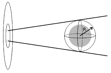
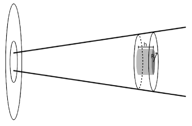
Figure 1: Sketch of both simulated volumes. Not to scale. $R$ represents the radius of a sphere or a disk and $h$ the height of the disk. All variables are defined in the plasma frame.

We consider two emission region geometries in our modelling. A sphere and a thin disk. The former is a first approximation to an unknown shape of the emitting plasma whereas the latter tries to take into account a possible shape derived from some heating mechanisms, such as magnetic reconnection and shock acceleration. In 1 we show a simple sketch of both volumes.

It should be noted that one of the basic assumptions of blazar modelling in general is that the emission zone is homogeneous and isotropic as all the equations for particle interactions assume isotropy at the interaction point. Although the effect is smaller for a sphere than a disk model, any choice of geometry will introduce an inherent anisotropy, the study of which lies beyond the scope of this work.

2.1.1 Sphere

The Spherical model (1 left) is defined by one characteristic length: the radius of the blob $R$. The free escape timescale, that is, the time a particle that does not interact in the volume takes to escape, $\left(\tau_{free,esc}\right)$ is then set as the average length that a particle would have to traverse to escape from a sphere divided by $c$:

$$\tau_{free,esc}=\frac{1}{c}\frac{\int_{V}\frac{\int_{\Omega}L\left(r,\Omega\right)d\Omega}{4\pi}dV}{\frac{4\pi}{3}R^{3}}=\frac{3}{4}\frac{R}{c}.$$ (2)

2.1.2 Thin Disk

The Thin Disk model (1 right) is defined by two characteristic lengths: the radius of the disk $\left(R\right)$ and the height of the disk $\left(h\right)$. The first order approximation to the escape timescale is:

$$\tau_{free,esc}=\frac{1}{c}\frac{\int_{V}\frac{\int_{\Omega}L\left(r,\Omega\right)d\Omega}{4\pi}dV}{\pi R^{2}h}\approx\frac{\pi}{4}\frac{h}{c}.$$ (3)

2.2 Kinetic equation approach to emission

The model we employ solves the coupled kinetic equations for $12$ different species of particles: protons, neutrons, electrons, charged and neutral pions, muons and antimuons, and electron and muon neutrinos and antineutrinos. The general form of a kinetic equation, omitting the linear term follows:

$$\frac{\partial n}{\partial t}=\mathcal{Q}_{ext}+\mathcal{Q}_{int}+\mathcal{L}-\frac{n}{\tau_{esc}}-\frac{n}{\tau_{dec}}+S\frac{\partial}{\partial\gamma}\left[\gamma^{2}n\right].$$ (4)

As shown in LABEL:Eq:kinetic_equation, the variation of the population of a species of particle is due to: external injection $\mathcal{Q}_{ext}$; internal injection $\mathcal{Q}_{int}$, which represents particles produced by processes internal to the simulated volume; loss of particles $\mathcal{L}$ due to interactions with other particles; an escape term where $\tau_{esc}$ represents the timescale for escaping the simulated volume, which we take as a multiple of the free timescale $\left(\tau_{esc}=\sigma\tau_{free,esc}\right)$; a decay term where $\tau_{dec}$ represents the decay timescale; and a continuous loss of energy where the energy lost is proportional to $\gamma^{2}$, such as synchrotron losses for charged particles and the Inverse Compton (IC) process for electrons. Lorentz factor $\gamma$ corresponds to the energy of a particle normalized to its rest mass energy $\left(\gamma=E/mc^{2}\right)$.

Usually, the expressions for photon injection and losses are given in terms of emission and absorption coefficients $\left(j_{\nu}\text{ and }\alpha_{\nu}\right)$. These are related according to:

$$\mathcal{Q}_{int} \equiv\left|\frac{\partial n_{\gamma}\left(\varepsilon\right)}{\partial t}\right|_{inj}=\frac{4\pi}{\varepsilon m_{e}c^{2}}\frac{d\nu}{d\varepsilon}j_{\nu}\left(\nu\right)=\frac{2}{\hbar\varepsilon}j_{\nu}\left(\nu\right),$$ (5)

$$\mathcal{L} \equiv\left|\frac{\partial n_{\gamma}\left(\varepsilon\right)}{\partial t}\right|_{abs}=c\alpha_{\nu}\left(\nu\right)n_{\gamma}\left(\varepsilon\right),$$ (6)

where $\hbar$ is the reduced Plank constant. For charged particle losses, an energy loss term of arbitrary strenght $\left(S\right)$ specializes according to

$$S\frac{\partial}{\partial\gamma}\left[\gamma^{2}n\right] =\frac{\partial}{\partial\gamma}\left[\frac{\partial\gamma}{\partial t}n\right],$$ (7)

In our model, all the charged particles create synchrotron emission, have synchrotron losses and cause synchrotron absorption. For this, we model the emission as:

$$j_{\nu}=\frac{1}{4\pi}\int_{1}^{\infty}n\left(\gamma\right)P_{\nu}\left(\gamma\right)d\gamma,$$ (8)

where $P_{\nu}\left(\gamma\right)$ is the energy emitted by a particle with energy $\gamma$ at frequency $\nu$ and has the form (Crusius & Schlickeiser, 1986):

$$P_{\nu}\left(\gamma\right)=\frac{\sqrt{3}}{4\pi}\frac{q^{3}B}{mc^{2}}xCS\left(x\right),$$ (9)

where $q$ and $m$ are the charge and the mass of the emitting particle, $B$ is the magnetic field strength, $x$ is the frequency normalized to a critical frequency $x=\nu/\nu_{c}$ with

$$\nu_{c}\equiv\nu_{0}\gamma^{2}\equiv\frac{3}{4\pi}\frac{qB}{mc}\gamma^{2},$$ (10)

and $CS\left(x\right)$ is a function given in terms of Whittaker functions:

$$CS\left(x\right)=W_{0,\frac{4}{3}}\left(x\right)W_{0,\frac{1}{3}}\left(x\right)-W_{\frac{1}{2},\frac{5}{6}}\left(x\right)W_{-\frac{1}{2},\frac{5}{6}}\left(x\right).$$ (11)

The loss of energy of the emitting particles is modelled as:

$$\frac{\partial\gamma}{\partial t}=-\frac{4}{3}c\sigma_{T}\frac{u_{B}}{m_{e}c^{2}}\left(\frac{m_{e}}{m}\right)^{3}\gamma^{2},$$ (12)

where $\sigma_{T}$ is the Thomson cross-section and $u_{B}$ is the energy density of the magnetic field.

The absorption of photons is modelled as:

$$\alpha_{\nu}=-\frac{1}{8\pi m\nu^{2}}\int_{1}^{\infty}\gamma^{2}\frac{\partial}{\partial\gamma}\left[\frac{n}{\gamma^{2}}\right]P_{\nu}\left(\gamma\right)d\gamma.$$ (13)

Photons interact with energetic electrons due to the inverse Compton process, which we model as:

$$j_{\nu}\left(\varepsilon_{s}\right)=\frac{\hbar\varepsilon_{s}}{2}\int_{1}^{\infty}n_{e}\left(\gamma_{e}\right)\int_{0}^{\infty}n_{\gamma}\left(\varepsilon\right)g_{u,d}\left(\gamma_{e},\varepsilon,\varepsilon_{s}\right)d\varepsilon d\gamma_{e},$$ (14)

where $\varepsilon$ is the energy of a photon normalized with respect to the energy of a rest electron ($\varepsilon$ is the initial energy of the photon and $\varepsilon_{s}$ is the energy after the scattering), $n_{e}$ is the electron population, $n_{\gamma}$ is the photon population and $g_{u,d}\left(\gamma,\varepsilon,\varepsilon_{s}\right)$ are two functions referring to the upscattering and downscattering of photons which where calculated by Jones (Jones, 1968, equations 40 and 44):

$$g_{u}\left(\gamma,\varepsilon,\varepsilon_{s}\right) =\frac{3c\sigma_{T}}{4\gamma^{2}\varepsilon}\left[2q_{u}\ln q_{u}\right.$$

$$\left.+\left(1+2q_{u}\right)\left(1-q_{u}\right)+\frac{\varepsilon_{s}^{2}}{\gamma\left(\gamma-\varepsilon_{s}\right)}\frac{1-q_{u}}{2}\right]$$ (15)

$$\quad\text{if }q_{u}\leq 1\leq\frac{\varepsilon_{s}}{\varepsilon},\,\varepsilon_{s}<\gamma,$$

$$g_{d}\left(\gamma,\varepsilon,\varepsilon_{s}\right) =\frac{3c\sigma_{T}}{16\gamma^{4}\varepsilon}\left[\left(q_{d}-1\right)\left(1+\frac{2}{q_{d}}\right)-2\ln q_{d}\right]$$ (16)

$$\quad\text{if }\frac{1}{q_{d}}\leq 1\leq\frac{\varepsilon}{\varepsilon_{s}},$$

with

$$q_{u} =\frac{\varepsilon_{s}}{4\varepsilon\gamma\left(\gamma-\varepsilon_{s}\right)},$$ (17)

$$q_{d} =\frac{4\gamma{{}^{2}}\varepsilon_{s}}{\varepsilon}.$$ (18)

The loss term for photons can be obtained as:

$$\frac{\partial n_{\gamma}\left(\varepsilon\right)}{\partial t}=-n_{\gamma}\left(\varepsilon\right)\int_{1}^{\infty}n_{e}\left(\gamma_{e}\right)\mathcal{R}\left(\gamma_{e},\varepsilon\right)d\gamma_{e},$$ (19)

where $\mathcal{R}\left(\gamma_{e},\varepsilon\right)$ is the reaction rate of electrons of energy $\gamma_{e}$ with photons of energy $\varepsilon$ and can be found from integrating the Klein-Nishina cross section.

$$\mathcal{R}\left(\gamma_{e},\varepsilon\right) =\frac{3}{16}c\sigma_{T}\frac{1}{\beta\gamma_{e}^{2}\varepsilon^{2}}\left[-\frac{x}{4}+\frac{1}{4\left(x+1\right)}+\right.$$

$$\phantom{=\frac{3}{16}c\sigma_{T}\frac{1}{\beta\gamma_{e}^{2}\varepsilon^{2}}}\frac{\left(x^{2}+9x+8\right)}{2x}\ln\left(1+x\right)+$$ (20)

$$\phantom{=\frac{3}{16}c\sigma_{T}\frac{1}{\beta\gamma_{e}^{2}\varepsilon^{2}}}\left.2\operatorname{Li}_{2}\left(-x\right)\right]_{x_{M}}^{x_{m}},$$

where:

$$x_{m} =2\varepsilon\gamma_{e}\left(1+\beta\right), x_{M} =2\varepsilon\gamma_{e}\left(1-\beta\right),$$ (21)

and $\operatorname{Li}_{2}$ the dilogarithm.

Following Böttcher et al. (2012), we use the simplified prescription for the electron energy losses in inverse comptom scattering:

$$\frac{\partial\gamma}{\partial t}=-\frac{4}{3}c\sigma_{T}\frac{u_{\gamma}}{m_{e}c^{2}}\gamma^{2},$$ (22)

where $u_{\gamma}$ is the energy density of the photon field:

$$u_{\gamma}=m_{e}c^{2}\times\int_{0}^{\infty}\varepsilon n_{\gamma}\left(\varepsilon\right)d\varepsilon.$$ (23)

Photons can interact among themselves creating electron and positron pairs, which we model according to (Böttcher & Schlickeiser, 1997). Photon losses are modelled according to the fully integrated cross section in a similar way to the photon loss term for IC.

$$\mathcal{R}\left(x\right) =\frac{3\sigma_{T}}{4x^{2}}\left\{a-2xa+\operatorname{Li}_{2}\left(\frac{1-a}{2}\right)-\operatorname{Li}_{2}\left(\frac{1+a}{2}\right)-\right.$$

$$\phantom{=\frac{3}{4x^{2}}\quad}\left.\operatorname{atanh}\left(a\right)\left[-\ln\left(4x\right)-\frac{1}{x}-2x+2\right]\right\},$$ (24)

where $x=\varepsilon_{1}\varepsilon_{2}$, $a=\sqrt{1-\frac{1}{x}}$.

Hadrons (protons and neutrons) interact with photons producing hadronic resonances which ultimately decay in the form of hadrons and pions. To model this we follow the approximations of HÃŒmmer et al (Hümmer et al., 2010) in their SimB model. We diverge though in the calculations of the loss and self-injection term for hadrons as, instead of applying a cooling term, we model every process as a loss and where applicable, we reinject the corresponding hadron with reduced energies.

Neutrons, charged pions and muons decay, producing ultimately protons, electrons, positrons and neutrinos. To model these processes, we follow HÃŒmmer et al (Hümmer et al., 2010) for the decay of pions and Lipari et al (Lipari et al., 2007) for the decay of muons and the production of neutrinos.

For electron-positron pair production and pair annihilation we follow Böttcher & Schlickeiser (1997) and Svensson (1982) respectively. Bethe-Heitler pair production is implemented following the model of Kelner & Aharonian (2008).

Finally, we do not model other processes such as proton-proton interaction, heating of charged particles when absorbing photons and heating of electrons when downscattering photons because their impact is negligible relative to that of the processes included in our model.

2.3 Steady State Models

In our steady state model the populations of both electrons and protons do not evolve over time. This also covers a scenario where both are injected constantly over time with a fixed distribution that would lead to the same steady state distribution that we here fix from the outset.

The initial distribution of electrons is considered to be a broken power law and for protons a simple power law:

$$n_{e}\left(\gamma_{e}\right) \propto\begin{cases}A\gamma_{e}^{-p_{1}}&\text{if }\gamma_{e,min}<\gamma_{e}<\gamma_{e,break}\\ B\gamma_{e}^{-p_{2}}&\text{if }\gamma_{e,break}<\gamma_{e}<\gamma_{e,max}\end{cases},$$ (25)

$$n_{p}\left(\gamma_{p}\right) \propto C\gamma_{p}^{-p}\,\text{if }\gamma_{p,min}<\gamma_{p}<\gamma_{p,max},$$ (26)

where $A$, $B$ and $C$ are factors that normalize the distributions and can be calculated from the conditions:

$$\int_{\gamma_{e,min}}^{\gamma_{e,break}}A\gamma_{e}^{-p_{1}}+\int_{\gamma_{e,break}}^{\gamma_{e,max}}B\gamma_{e}^{-p_{2}}d\gamma_{e} =1,$$ (27)

$$A\gamma_{e,break}^{-p_{1}} =B\gamma_{e,break}^{-p_{2}},$$ (28)

$$\int_{\gamma_{p,min}}^{\gamma_{p,max}}C\gamma_{p}^{-p}d\gamma =1,$$ (29)

and we have:

$$A \approx\left(p_{1}-1\right)\gamma_{e,min}^{p_{1}-1},$$ (30)

$$B =A\gamma_{e,break}^{p_{2}-p_{1}},$$ (31)

$$C \approx\left(p-1\right)\gamma_{p,min}^{p-1}.$$ (32)

We can assume that the ratio of protons to electrons is given by $\eta$. This means that, given a combined mass density $\rho$ of accelerated electrons and protons, the steady populations for electrons and protons are:

$$n_{e}\left(\gamma_{e}\right) =\frac{\rho}{m_{e}+\eta\,m_{p}}A\times$$

$$\begin{cases}\phantom{\gamma_{e,break}^{p_{2}-p_{1}}}\gamma_{e}^{-p_{1}}&\text{if }\gamma_{e,min}<\gamma_{e}<\gamma_{e,break}\\ \gamma_{e,break}^{p_{2}-p_{1}}\gamma_{e}^{-p_{2}}&\text{if }\gamma_{e,break}<\gamma_{e}<\gamma_{e,max}\end{cases},$$ (33)

$$n_{p}\left(\gamma_{p}\right) =\frac{\eta\,\rho}{m_{e}+\eta\,m_{p}}C\times\gamma_{p}^{-p}.$$ (34)

Initially, in the simulated volume there are only electrons and protons, so we need to evolve the plasma until it reaches a ’true’ steady state for all the particles. This is detected by calculating a statistic related to the relative change in population of particles with time which is then compared with a selected tolerance:

$$\sqrt{\int\left[\frac{1}{n\left(x\right)}\frac{\partial n\left(x\right)}{\partial t}\right]^{2}dx}<\text{tol},$$

where $n$ is the kind of particles we are interested in. In our case, we test three particles species for convergence: photons, electrons and neutrinos.

We consider that the system has reached the photonic steady state when the photon statistic has a value lower than $10^{-8}$, and the final steady state when all three have a value lower than $10^{-8}$. The value $10^{-8}$ has been chosen as a good compromise between the accuracy of the steady state and the simulation time, given that the system only asymptotically approaches a true steady state. We check the photon, neutrino and electron populations for convergence for the following reasons. The photon population directly shapes the SED, the electron population has a long covergence timescale especially at low energies due to cooling, and neutrinos are the last particles to be produced and therefore formally the last to achieve steady state.

It takes time for the plasma to settle into a converged state, and this time scale should be consistent with the variability time scale of the conditions in the plasma as inferred from the blazar light curve. In our application to TSX0506+056, we have verified that our results are consistent with the 91 days time scale as experienced by the plasma blob. We note that our modeled physical time scales for the evolution from scratch to full convergence are an overestimate resulting from uncertainties on both ends of the process. In reality, there will likely be an initial distribution of energetic particles prior to the onset of the flare, while the observed SED does not necessarily show a completely converged state.

The steady state for protons and electrons is implemented by choosing not to update their populations during the evolution of the system. We can use this fact to have an a priori value for the energy density in protons and electrons:

$$u_{e} =m_{e}c^{2}\times\int_{\gamma_{e,min}}^{\gamma_{e,max}}\gamma_{e}n_{e}\left(\gamma_{e}\right)d\gamma_{e},$$ (35)

$$u_{p} =m_{p}c^{2}\times\int_{\gamma_{p,min}}^{\gamma_{p,max}}\gamma_{p}n_{e}\left(\gamma_{p}\right)d\gamma_{p}.$$ (36)

2.4 Dynamic Models

Dynamic models break the assumption of a steady state population of electrons and protons by allowing them to evolve over time. To arrive at a steady state population of particles we have two options: we can inject particles arriving from outside the volume with a given distribution, or we can keep a steady population of cold particles that are accelerated to higher energies within the volume. In this work we focus on the first option. There are various reasons for this. One is that acceleration introduces various parameters, the acceleration timescales and mechanisms, which are not well understood. Second, the accelerated particles have to come from a population of cold particles, which we do not model. Third, acceleration requires a bit of tuning to obtain the right slope and enough maximum energy for the particle populations. Fourth, one can argue that acceleration is only going to happen at the boundaries of the simulated volume (e.g. shock fronts), and thus, its effect is to inject energetic particles with a given distribution to the rest of the volume.

Particle injection is characterized by a luminosity ($L$) and a normalized particle distribution $f\left(\gamma\right)$ such that:

$$\frac{L}{Vmc^{2}}=\int_{\gamma_{min}}^{\gamma_{max}}\gamma\mathcal{Q}_{ext,0}f\left(\gamma\right)d\gamma,$$ (37)

where $V$ is the volume of the plasma where the injection is happening, $m$ is the mass of the injected particle and $\mathcal{Q}_{ext,0}$ is the number density of injected particles. For a known particle distribution, we can solve for $\mathcal{Q}_{ext,0}$ as:

$$\mathcal{Q}_{ext,0}=\frac{L}{\left\langle\gamma\right\rangle Vmc^{2}},$$ (38)

where $\left\langle\gamma\right\rangle$ is the average energy of the injected particles. In our case, we inject electrons and protons. Assuming that the ratio of injected protons to electrons is $\eta$, we have:

$$\frac{L}{V} =\mathcal{Q}_{ext,e,0}\left\langle\gamma_{e}\right\rangle m_{e}c^{2}+\eta\mathcal{Q}_{ext,e,0}\left\langle\gamma_{p}\right\rangle m_{p}c^{2},$$ (39)

$$Q_{e,0} =\frac{L/V}{\left\langle\gamma_{e}\right\rangle m_{e}c^{2}+\eta\left\langle\gamma_{p}\right\rangle m_{p}c^{2}},$$ (40)

and thus:

$$Q_{e}\left(\gamma_{e}\right) =\phantom{\eta}\mathcal{Q}_{ext,e,0}f_{e}\left(\gamma_{e}\right),$$ (41)

$$Q_{p}\left(\gamma_{p}\right) =\eta\mathcal{Q}_{ext,e,0}f_{p}\left(\gamma_{p}\right).$$ (42)

Once a steady state is achieved and assuming that the injection follows a broken power law, simplified versions of the kinetic equations can be applied to obtain an approximation to the final electron and proton populations.

For low energies, we have that the cooling time due to synchrotron and Inverse Compton processes is longer than the escape timescale of the particles. This means that we can approximate the population evolution as:

$$\frac{\partial n}{\partial t}\approx\mathcal{Q}_{ext}-\frac{n}{\tau_{esc}}.$$ (43)

By taking the derivative equal to $0$, we obtain that in the steady state limit the population is:

$$n \approx\mathcal{Q}_{ext}\tau_{esc},$$ (44)

$$n_{e}\left(\gamma_{e}\right) \approx\mathcal{Q}_{ext,e,0}\tau_{esc}A\times$$

$$\begin{cases}\phantom{\gamma_{e,break}^{p_{2}-p_{1}}}\gamma_{e}^{-p_{1}}&\text{if }\gamma_{e,min}<\gamma_{e}<\gamma_{e,break}\\ \gamma_{e,break}^{p_{2}-p_{1}}\gamma_{e}^{-p_{2}}&\text{if }\gamma_{e,break}<\gamma_{e}<\gamma_{e,max}\end{cases},$$ (45)

$$n_{p}\left(\gamma_{p}\right) \approx\eta Q_{e,0}\tau_{esc}C\times\gamma_{p}^{-p}.$$ (46)

If a steady state is achieved from dynamically injected protons and electrons, the dynamic model and the steady state model relate according to:

$$\frac{L\tau_{esc}/V}{\left\langle\gamma_{e}\right\rangle m_{e}c^{2}+\eta\left\langle\gamma_{p}\right\rangle m_{p}c^{2}} \approx\frac{\rho}{m_{e}+\eta\,m_{p}}.$$ (47)

For higher energies where we can not ignore the effects of synchrotron cooling and Inverse Compton losses, we can approximate the population with a power law with a given index $p$. We obtain:

$$\frac{\partial n}{\partial t} \approx\mathcal{Q}_{ext}+n_{0}\gamma^{-p}\left[\left(2-p\right)\gamma S-\frac{1}{\tau_{esc}}\right].$$ (48)

In the steady state, we obtain:

$$n_{0}\gamma^{-p} \approx\frac{\mathcal{Q}_{ext}\tau_{esc}}{1-\left(2-p\right)\gamma S\tau_{esc}}.$$ (49)

For $\left(2-p\right)\gamma S\tau_{esc}\ll 1$ we recover the previous result where we ignored the contributions of Synchrotron and Inverse Compton cooling. When $\left(2-p\right)\gamma S\tau_{esc}\gg 1$ we obtain that the main driver of the population is cooling, and we get:

$$n_{0}\gamma^{-p} \approx\frac{1}{p-2}\frac{\mathcal{Q}_{ext}}{\gamma S},$$ (50)

$$n_{e}\left(\gamma_{e}\right) \approx\frac{1}{p-2}\frac{\mathcal{Q}_{ext,e,0}}{S}A\times$$

$$\begin{cases}\phantom{\gamma_{e,break}^{p_{2}-p_{1}}}\gamma_{e}^{-p_{1}-1}&\text{if }\gamma_{e,min}<\gamma_{e}<\gamma_{e,break}\\ \gamma_{e,break}^{p_{2}-p_{1}}\gamma_{e}^{-p_{2}-1}&\text{if }\gamma_{e,break}<\gamma_{e}<\gamma_{e,max}\end{cases},$$ (51)

$$n_{p}\left(\gamma_{p}\right) \approx\frac{1}{p-2}\frac{\eta\mathcal{Q}_{ext,e,0}}{S}C\times\gamma_{p}^{-p_{inj}-1},$$ (52)

where we see that the effect that cooling produces is to increase the index of the injected distribution of particles by $1$.

Particles with energies lower than the minimum energy of the injected energy can appear due to cooling. If the turnover energy in a charged particle population due to cooling lies below the level associated with the lower injection cut-off Lorentz factor, an intermediate regime appears in the particle spectrum. In the absence of additional physical processes, this would lead to a power law slope of 2. Below the turnover energy, escape takes over from cooling as the main driver, which leads to a drop in the population.

3 Bayesian and Markov Chain Monte Carlo analysis

Model fitting can be done in various ways. An easy and straightforward way of doing it is by eye (Keivani et al., 2018), where the goodness of the fit is estimated by seeing if the simulated spectrum fits the observations. The disadvantages of this approach are that the validity of the fit can not be validated numerically and that, depending on the parameters, finding a good fit might be a complicated task.

Another way is by performing grid searches (Gao et al., 2019), where the parameter space is divided into a grid, and, for every point in this grid you assign a goodness of fit value, taking the best parameters as the final ones. This has the advantage of being fully automated but has the disadvantage of requiring a high amount of computations, as quite a lot of time is spent calculating the likelihood of bad parameters.

A third method, similar to the latter, is to perform an MCMC search over the parameter space (see for example Qin et al. (2018) for a study that employed MCMC to fit simple leptonic models to blazars). In this case, instead of dividing the parameter space into a grid and checking every point, a series of ’walkers’ traverse the parameter space checking the likelihood of the fit at the point where they are. Their advance is biased towards improving the likelihood so as to guide their search towards ’good’ parameters. Nevertheless, the search is ergodic, which means that with time, the whole parameter space will be traversed. Just like the previous method, MCMC searches are fully automated, but they have the advantage of being focused on the best parameters. This allows us to obtain two results besides the best parameters. On the one hand, it allows us to obtain a measure of the error in each of the parameters. On the other hand, a study of the behaviour of the MCMC walkers allows us to identify correlations between the parameters. This in turn allows us to redefine our parameters so as to eliminate the correlations between them and improve the fits. It should be noted that not all MCMC sampling algorithms perform worse under correlated parameters. Nevertheless, finding good ’fit parameters’ a priori can give a very useful physical insight in the interconnectedness of the model parameters.

Therefore, we will refer to two sets of parameters: ’model parameters’, or simply parameters, which are the input of our model; and ’fitted parameters’, which are the set that MCMC fits. Both sets are related by invertible transformations, so it is easy to go from one to other.

MCMC requires some information from our part to perform its search. Just as grid search needs a grid to be defined, MCMC needs information about the distribution of the parameters it has to fit. The priors on the fitted parameters are derived by starting from flat priors in either linear or logarithmic space of the model parameters. The distributions are chosen so that parameters that enter the model as multiplicative terms are defined in logarithmic space and parameters that enter as exponents are defined in linear space. The limits of the distributions are taken very loosely, even to the point where in some cases we allow unphysical values. The only hard limits are the relations $\gamma_{e,min}<\gamma_{e,break}<\gamma_{e,max}$ and $p_{1}<p_{2}$, and in the case of thin shells, $h<R$.

The log-likelihood of the model is calculated as:

$$l=-\frac{1}{2}\sum_{n}\left(\frac{y_{n}-\hat{y}_{n}}{\sigma_{n}}\right)^{2},$$ (53)

where $y_{n}$ are the observations, $\hat{y}_{n}$ are the predictions of our model and $\sigma_{n}$ are the errors of the observations, which we assume to be a few percent of the observations, depending on the observed band. In our case, we take that for optical frequencies, we have $\sigma_{n}=0.1\,y_{n}$; for X-rays $\sigma_{n}=0.2\,y_{n}$; and for gamma-rays $\sigma_{n}=0.5\,y_{n}$.

The log-likelihood of the ’fitted parameters’ is then defined as a combination of the log-likelihood of the model plus the a-priori log-likelihood of the ’fitted parameters’. Denoting the ’model parameters’ as $P$ the ’fitted parameters’ as $F$ and the a-priori log-likelihood of a set of parameters as $p\left(X\right)$, we obtain:

$$\mathcal{L}\left(F\right) =l\left(F\right)+p\left(F\right)$$

$$=l\left(F\right)+p\left(P\right)-\ln\left(\left|\frac{dF}{dP}\right|\right)$$

$$=l\left(F\right)-\ln\left(\left|\frac{dF}{dP}\right|\right),$$ (54)

where the term $\left|dF/dP\right|$ represents the Jacobian of the transformation between parameters, and $p\left(P\right)=0$ by construction.

In our implementation, we use an affine invariant sampler (Goodman & Weare, 2010) implemented in the Python package emcee (Foreman-Mackey et al., 2013) using 128 walkers. The total numbers of samples taken differ between runs and are reported along with the outcomes of a run.

The first data points of each walker correspond to the period of ’burn in’, where the walkers spread from their initial conditions until they explore the log-likelihood function in an uncorrelated way. During each of the runs, the data is binned and the values of the average, median, standard deviation and 16 and 84 percentiles are checked for trends. After they remain consistent for several bins we consider that the run has found the final distribution and the run is stopped.

The bins where the aforementioned values drift are considered the ’burn-in’ phase and their data discarded for the final study.

As an additional consistency check for the remaining data. We rebin the data and plot the PDFs to verify that the features of the distributions remain essentially unchanged when drawn from subsets of the full chain.

While it is never formally possible to rule out trends with an extremely long correlation time, we are therefore confident that the results do not contain biases.

All the results reported in tables correspond to the median and the 16 and 84 percentiles.

4 Applying our models in a Bayesian framework

Before trying to fit a data set, we do an a priori analysis of the physics of the emission processes in order to obtain constraints and correlations for our parameters. These relations are then used to find good initial parameters for the MCMC analysis and to interpret the outcome of the fitting process.

4.1 Initial Assumptions and Constraints

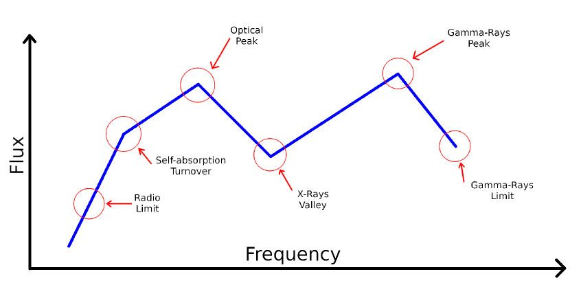
Figure 2: Schematic view of a blazar SED with some interesting points marked for clarity.

LABEL:Fig:Schematic-SED shows a simple schematic view of an SED, which we can use to obtain a series of constraints and first guesses for our search:

• We can assume that the first peak of the SED is near the optical band, and that it is caused by the synchrotron emission of the electrons at the break point $\gamma_{e,break}$. This gives us the constraint:

  $$\nu_{obs,opt}\approx\frac{3}{4\pi}\frac{qB}{m_{e}c}\gamma_{e,break}^{2}\frac{\delta}{1+z}.$$ (55)

• We know that we have to obtain photons of a certain energy, and that those come from the Inverse Compton process with high energy electrons. So, we can derive a lower limit for the maximum value of $\gamma_{e,max}$:

  $$\nu_{obs,max}\lesssim\gamma_{e,max}\frac{m_{e}c^{2}}{2\pi\hbar}\frac{\delta}{1+z}.$$ (56)

• A second lower limit for the value of $\gamma_{e,max}$, albeit much less limiting, can be obtained from the X-ray valley. We can safely assume that the emission for the low energy part of the valley comes almost entirely from the synchrotron emission of high energy electrons. This gives us the constraint:

  $$\nu_{obs,xray}\lesssim\frac{3}{4\pi}\frac{qB}{m_{e}c}\gamma_{e,max}^{2}\frac{\delta}{1+z}.$$ (57)

• We can fit a line between the optical and the X-ray emission. As it is above the synchrotron peak, we can assume that this emission comes from electrons with $\gamma_{e}>\gamma_{e,break}$ and, as the theoretical slope of synchrotron emission is known, we can find the constraint:

  $$\frac{3-p_{2}}{2}\approx\alpha_{2}.$$ (58)

• We can fit a line between the X-ray emission and Gamma-ray emission, and we can assume that the emission in this range is going to be caused by the upscattering of synchrotron photons by the Inverse Compton process. The inverse Compton process increases the energy of photons as $\varepsilon_{after}\approx\gamma_{e}^{2}\varepsilon_{before}$. For photons from the synchrotron peak, upscattered by electrons at $\gamma_{e,break}$, their energy is above the fit. So, these photons should come from synchrotron photons emitted by electrons with $\gamma_{e}<\gamma_{e,break}$.
  As the Inverse Compton process does not modify the slope of the emission, we obtain:

  $$\frac{3-p_{1}}{2}\approx\alpha_{1}.$$ (59)

• The radio observations can be considered as upper limits for our model, as the flux can come from the extended emission in the jet (see for example Cerruti et al. 2018). From this fact, we can derive another constraint. Assuming, as before, that the optical observations are the peak of the synchrotron spectrum, and that they are caused by electrons with energy $\gamma_{e,break}$, we can extrapolate the observations down to the frequency associated with $\gamma_{e,min}$:

  $$\left(\nu F_{\nu}\right)_{break}=A\nu_{break}^{\alpha_{1}},$$ (60)

  so:

  $$\left(\nu F_{\nu}\right)_{min}=\left(\nu F_{\nu}\right)_{break}\left(\frac{\nu_{min}}{\nu_{break}}\right)^{\alpha_{1}}.$$ (61)

  At lower frequencies, this can be extrapolated further using the index $4/3$. And we obtain:

  $$\left(\nu F_{\nu}\right)_{min} =B\nu_{min}^{4/3},$$ (62)

  $$B =\left(\nu F_{\nu}\right)_{break}\frac{\nu_{min}^{\alpha_{1}-4/3}}{\nu_{break}^{\alpha_{1}}},$$ (63)

  so:

  $$\left(\nu F_{\nu}\right)_{radio}=\left(\nu F_{\nu}\right)_{break}\left(\frac{\nu_{min}}{\nu_{break}}\right)^{\alpha_{1}}\left(\frac{\nu_{radio}}{\nu_{min}}\right)^{4/3}.$$ (64)

  Now, all the frequencies can be transformed into associated gamma factors for electrons in the fluid frame:

  $$\left(\nu F_{\nu}\right)_{radio}=\left(\nu F_{\nu}\right)_{break}\left(\frac{\gamma_{e,min}}{\gamma_{e,break}}\right)^{2\alpha_{1}}\left(\frac{\gamma_{e,radio}}{\gamma_{e,min}}\right)^{8/3}.$$ (65)

  Note that $\gamma_{e,radio}$ is not a real value for the gamma factor of electrons, as it can be $<1$. Also note that it might be the case that the synchrotron self absorption frequency is higher than the frequency associated with $\gamma_{e,min}$. In this case, by using $\gamma_{e,min}$ we would be overestimating the approximation of $\left(\nu F_{\nu}\right)_{radio}$. The constraint is that the observed flux in radio has to be less than the calculated, so:

  $$\left(\nu F_{\nu}\right)_{radio,obs}\gtrsim\left(\nu F_{\nu}\right)_{break,obs}\left(\frac{\gamma_{e,min}}{\gamma_{e,break}}\right)^{2\alpha_{1}}\left(\frac{\gamma_{e,radio}}{\gamma_{e,min}}\right)^{8/3}.$$ (66)

• The energy of the photons at the optical band is enough so that the blob can be considered thin to the radiation. In this case, the main loss term for photons is escape. Under the simplification of a $\delta$-approximation to synchrotron emission (Böttcher et al., 2012, Chapter 3), which we only employ here in order to make an estimate, we have:

  $$j_{\nu}\left(\nu\right)=\frac{1}{6\pi}c\sigma_{T}u_{B}\sqrt{\frac{\nu}{\nu_{0}}}\frac{1}{\nu_{0}}n_{e}\left(\gamma_{e}=\sqrt{\frac{\nu}{\nu_{0}}}\right).$$ (67)

  The emission coefficient is related to the rate of injection of photons as:

  $$\left|\frac{\partial n_{\gamma}\left(\varepsilon\right)}{\partial t}\right|_{inj}=\frac{4\pi}{\varepsilon m_{e}c^{2}}\frac{d\nu}{d\varepsilon}j_{\nu}\left(\nu\right)=\frac{2}{\hbar\varepsilon}j_{\nu}\left(\nu\right).$$ (68)

  The $\delta$-approximation also allows us to have that $\sqrt{\nu/\nu_{0}}=\gamma_{e}$, and thus, we can relate $\nu$, $\varepsilon$ and $\gamma_{e}$ as:

  $$\varepsilon=\frac{2\pi\hbar\nu}{m_{e}c^{2}}=\frac{2\pi\hbar\nu_{0}}{m_{e}c^{2}}\gamma_{e}^{2},$$ (69)

  which means that:

  $$\left|\frac{\partial n_{\gamma}\left(\varepsilon\right)}{\partial t}\right|_{inj} =\frac{m_{e}c^{2}}{\hbar^{2}\nu_{0}^{2}}\frac{1}{6}c\sigma_{T}u_{B}\frac{1}{\gamma_{e}}n_{e}\left(\gamma_{e}\right).$$ (70)

  As the main losses for photons is the escape term we have:

  $$\frac{\partial n_{\gamma}\left(\varepsilon\right)}{\partial t}=\frac{m_{e}c^{2}}{\hbar^{2}\nu_{0}^{2}}\frac{1}{6}c\sigma_{T}u_{B}\frac{1}{\gamma_{e}}n_{e}\left(\gamma_{e}\right)-\frac{n_{\gamma}\left(\varepsilon\right)}{\tau_{esc}}.$$ (71)

  In the steady state, $\partial n/\partial t=0$, so, we can solve for the equilibrium population of photons as:

  $$n_{\gamma}\left(\varepsilon\right)=\tau_{esc}\frac{m_{e}c^{2}}{\hbar^{2}\nu_{0}^{2}}\frac{1}{6}c\sigma_{T}u_{B}\frac{1}{\gamma_{e}}n_{e}\left(\gamma_{e}\right).$$ (72)

  The electron population is related to the density of the blob and we have, assuming that $\gamma_{e,min}\ll\gamma_{e,break}$:

  $$n_{\gamma}\left(\varepsilon\right) =\tau_{esc}\frac{m_{e}c^{2}}{\hbar^{2}\nu_{0}^{2}}\frac{1}{6}c\sigma_{T}u_{B}$$

  $$\phantom{=\;}\frac{1}{\gamma_{e}}\frac{\rho}{m_{e}+\eta m_{p}}\left(p_{1}-1\right)\gamma_{e,min}^{p_{1}-1}\gamma_{e}^{-p_{1}},$$ (73)

  for $\gamma_{e}\leq\gamma_{e,break}$.
  The transformation from population to observed flux requires us to multiply the previous expression by $\varepsilon^{2}$, which we do using the relation with $\gamma_{e}$:

  $$\varepsilon^{2}n_{\gamma}\left(\varepsilon\right) =\tau_{esc}\frac{1}{m_{e}c^{2}}\frac{c\sigma_{T}}{12\pi}B^{2}$$

  $$\phantom{=\;}\frac{\rho}{m_{e}+\eta m_{p}}\left(p_{1}-1\right)\gamma_{e,min}^{p_{1}-1}\gamma_{e}^{3-p_{1}}.$$ (74)

  Doing the final transformation we have:

  $$\nu F_{\nu} =\frac{\delta^{4}}{4\pi\left(1+z\right)D_{L}^{2}}V\frac{c\sigma_{T}}{12\pi}B^{2}$$

  $$\phantom{=\;}\frac{\rho}{m_{e}+\eta m_{p}}\left(p_{1}-1\right)\gamma_{e,min}^{p_{1}-1}\gamma_{e}^{3-p_{1}}$$ (75)

  $$\propto\delta^{4}VB^{2}\rho\left(p_{1}-1\right)\gamma_{e,min}^{p_{1}-1}\gamma_{e}^{3-p_{1}}.$$

  It is important to remember that this is only valid for energies where the blob is not thick to the radiation, and only for $\gamma<\gamma_{e,break}$.

• Following the previous point, we can also derive the flux for the low energy part of the x-ray band, as we assume that those photons are synchrotron emission from high energy electrons. The population of high energy electrons is:

  $$n_{e}\left(\gamma_{e}>\gamma_{e,break}\right) =\frac{\rho}{m_{e}+\eta m_{p}}\left(p_{1}-1\right)$$

  $$\phantom{=\;}\gamma_{e,min}^{p_{1}-1}\gamma_{e,break}^{p_{2}-p_{1}}\gamma_{e}^{-p_{2}}.$$ (76)

  Then, the photon population for the high energy part of the synchrotron spectrum is:

  $$n_{\gamma}\left(\varepsilon\right) =\tau_{esc}\frac{m_{e}c^{2}}{\hbar^{2}\nu_{0}^{2}}\frac{1}{6}c\sigma_{T}u_{B}$$

  $$\phantom{=\;}\frac{1}{\gamma_{e}}\frac{\rho}{m_{e}+\eta m_{p}}\left(p_{1}-1\right)\gamma_{e,min}^{p_{1}-1}\gamma_{e,break}^{p_{2}-p_{1}}\gamma_{e}^{-p_{2}}.$$ (77)

  for $\gamma_{e}>\gamma_{e,break}$. So, the X-Ray flux is:

  $$\nu F_{\nu} =\frac{c\sigma_{T}}{48\pi^{2}}\frac{\delta^{4}V}{\left(1+z\right)D_{L}^{2}}B^{2}$$

  $$\phantom{=\;}\frac{\rho}{m_{e}+\eta m_{p}}\left(p_{1}-1\right)\gamma_{e,min}^{p_{1}-1}\gamma_{e,break}^{p_{2}-p_{1}}\gamma_{e}^{3-p_{2}}$$ (78)

  $$\propto V\delta^{4}B^{2}\gamma_{e,x-ray}^{3}\rho\left(p_{1}-1\right)\gamma_{e,min}^{p_{1}-1}\gamma_{e,break}^{p_{2}-p_{1}}\gamma_{e,x-ray}^{-p_{2}}.$$

  Following one of our previous constraints, $\gamma_{e,x-ray}\lesssim\gamma_{e,max}$, so:

  $$\nu F_{\nu}\gtrsim V\delta^{4}B^{2}\rho\left(p_{1}-1\right)\gamma_{e,min}^{p_{1}-1}\gamma_{e,break}^{p_{2}-p_{1}}\gamma_{e,max}^{3-p_{2}}.$$ (79)

  Dividing our previous prediction for optical flux and X-rays flux, we have:

  $$\frac{\left(\nu F_{\nu}\right)_{optical}}{\left(\nu F_{\nu}\right)_{x-rays}}\sim\frac{\gamma_{e,break}^{3-p_{1}}}{\gamma_{e,break}^{p_{2}-p_{1}}\gamma_{e,max}^{3-p_{2}}}\sim\left(\frac{\gamma_{e,break}}{\gamma_{e,max}}\right)^{3-p_{2}}.$$ (80)

• Photons from synchrotron processes get upscattered by high energy electrons due to Inverse Compton processes. As an approximation, and just so we can derive a functional form for the photon population at high energies, we can say that the emission coefficient for IC photons depends on the population of photons at low energy and the population of electrons at high energy. As before, we assume that the energy of a photon is increased as $\varepsilon_{after}\approx\gamma_{e}^{2}\varepsilon_{before}$.

  $$j_{\nu,IC}\left(\varepsilon\right)=\frac{c\sigma_{T}}{4}\hbar n_{\gamma}\left(\frac{\varepsilon}{\gamma_{e}^{2}}\right)n_{e}\left(\gamma_{e}\right).$$ (81)

  Transforming to the rate of injection of photons, we obtain:

  $$\left|\frac{\partial n_{\gamma}\left(\varepsilon\right)}{\partial t}\right|_{inj}=\frac{c\sigma_{T}}{2}\frac{1}{\varepsilon}n_{\gamma}\left(\frac{\varepsilon}{\gamma_{e}^{2}}\right)n_{e}\left(\gamma_{e}\right).$$ (82)

  Again, we assume that the main losses are the escape process, so we can calculate the population of gamma ray photons in our blob as:

  $$n_{\gamma}\left(\varepsilon\right)=\tau_{esc}\frac{c\sigma_{T}}{2}\frac{1}{\varepsilon}n_{\gamma}\left(\frac{\varepsilon}{\gamma_{e}^{2}}\right)n_{e}\left(\gamma_{e}\right).$$ (83)

  To compare with the optical flux, we just multiply by $\varepsilon^{2}$:

  $$\varepsilon^{2}n_{\gamma}\left(\varepsilon\right)=\tau_{esc}\frac{c\sigma_{T}}{2}\varepsilon n_{\gamma}\left(\frac{\varepsilon}{\gamma_{e}^{2}}\right)n_{e}\left(\gamma_{e}\right).$$ (84)

  We assume that the photons that get upscattered to $\gamma$-rays are those from the synchrotron peak, and that the electrons with $\gamma_{e,break}$ are the ones mainly responsible for the upscattering. This means that $\varepsilon_{opt}\gamma_{e,break}^{2}=\varepsilon_{\gamma-ray}$ and $n_{\gamma}\left(\varepsilon_{opt}\right)=n_{\gamma}\left(\varepsilon_{\gamma-ray}/\gamma_{e,break}^{2}\right)$. This means that the ratio of fluxes is:

  $$\frac{\left(\nu F_{\nu}\right)_{\gamma-rays}}{\left(\nu F_{\nu}\right)_{opt}} =\frac{\left(\varepsilon^{2}n_{\gamma}\right)_{\gamma-rays}}{\left(\varepsilon^{2}n_{\gamma}\right)_{opt}},$$

  $$=\frac{m_{e}c^{2}}{2\pi\hbar\nu_{0}}\tau_{esc}\frac{c\sigma_{T}}{2}$$

  $$\phantom{=\;}\frac{\rho}{m_{e}+\eta m_{p}}\left(p_{1}-1\right)\gamma_{e,min}^{p_{1}-1}\gamma_{e,break}^{-p_{1}},$$ (85)

  $$\propto\frac{1}{\delta B}\tau_{esc}\rho\left(p_{1}-1\right)\gamma_{e,min}^{p_{1}-1}\gamma_{e,break}^{-p_{1}}.$$

4.2 Application to TXS0506+056: Initial Estimates

TXS 0506+056 is a Bl Lac kind of blazar where recently a neutrino was detected coincident with a flare, which established the importance of a hadronic component to blazar modelling. Due to this, there is a high amount of almost simultaneous data that we can use to test emission models.

Following 4.1, we can use the available observational data on TXS 0506+056 to estimate good initial values for our fitting procedure. Frequencies are given in $s^{-1}$ and fluxes in $erg\cdot s^{-1}\cdot cm^{-2}$. We have:

$$\nu_{obs,radio} \sim 10^{10}, \left(\nu F_{\nu}\right)_{obs,radio} \sim 10^{-13},$$

$$\nu_{obs,opt} \sim 10^{15}, \left(\nu F_{\nu}\right)_{obs,opt} \sim 4\times 10^{-11},$$

$$\nu_{obs,x-ray} \sim 10^{18}, \left(\nu F_{\nu}\right)_{obs,x-ray} \sim 10^{-12},$$

$$\nu_{obs,\gamma-ray} \sim 4\times 10^{23}, \left(\nu F_{\nu}\right)_{obs,\gamma-ray} \sim 6\times 10^{-11},$$

$$\nu_{obs,max} \sim 10^{26},$$

• By the constraint from (LABEL:nu_break_constraint) and the value for $\nu_{obs,opt}$ we obtain:

  $$\log_{10}\left(\delta B\gamma_{e,break}^{2}\right) \approx 8.50.$$ (86)

• By the constraint from (LABEL:gamma_max_constraint) and the value for $\nu_{obs,max}$ we obtain:

  $$\log_{10}\left(\delta\gamma_{e,max}\right) \gtrsim 6.03.$$ (87)

• By the constraint from (LABEL:gamma_max_constraint_xray) and the value for $\nu_{obs,x-ray}$ we obtain:

  $$\log_{10}\left(\delta B\gamma_{e,max}^{2}\right) \gtrsim 11.50.$$ (88)

• By the constraint from (LABEL:alpha_2_constraint) and the values for $\nu_{obs,opt}$, $\nu_{obs,x-ray}$, $\left(\nu F_{\nu}\right)_{obs,opt}$ and $\left(\nu F_{\nu}\right)_{obs,x-ray}$,we obtain:

  $$p_{2} \approx 4.06.$$ (89)

• By the constraint from (LABEL:alpha_1_constraint) and the values for $\nu_{obs,x-ray}$, $\nu_{obs,\gamma-ray}$, $\left(\nu F_{\nu}\right)_{obs,x-ray}$ and $\left(\nu F_{\nu}\right)_{obs,\gamma-ray}$,we obtain:

  $$p_{1} \approx 2.36.$$ (90)

• By the constraint from (LABEL:radio_constraints) and the values for $\nu_{obs,radio}$, $\nu_{obs,opt}$, $\left(\nu F_{\nu}\right)_{obs,radio}$ and $\left(\nu F_{\nu}\right)_{obs,opt}$,we obtain, assuming $\alpha_{1}\approx 1/3$ :

  $$\log_{10}\left(\delta B\gamma_{e,min}^{2}\right)\gtrsim 4.44.$$ (91)

• We have obtained a form for the optical flux in (LABEL:optical_flux_constraints). With the value for $\left(\nu F_{\nu}\right)_{obs,opt}$ we obtain:

  $$\log_{10}\left[\delta^{4}VB^{2}\rho\left(p_{1}-1\right)\gamma_{e,min}^{p_{1}-1}\gamma_{e,break}^{3-p_{1}}\right]\approx 37.83.$$ (92)

  and interestingly, combining the previous constraint with that for $\delta B\gamma_{e,break}^{2}$ we obtain:

  $$\log_{10}\left[\delta^{2}V\rho\left(p_{1}-1\right)\gamma_{e,min}^{p_{1}-1}\gamma_{e,break}^{-p_{1}-1}\right]\approx 20.83.$$ (93)

• From the relation between the $\gamma$-ray and the optical flux, (LABEL:g_ray_opt_constraints) we can obtain:

  $$\log_{10}\left[\frac{1}{\delta B}\tau_{esc}\rho\left(p_{1}-1\right)\gamma_{e,min}^{p_{1}-1}\gamma_{e,break}^{-p_{1}}\right]\approx-23.07.$$ (94)

• Dividing the optical flux reduced by $\left(\delta B\gamma_{e,break}^{2}\right)^{2}$ by the previous relation we obtain:

  $$\log_{10}\left(\delta^{3}B\frac{V}{\tau_{esc}}\gamma_{e,break}^{-1}\right)\approx 43.89.$$ (95)

• And reducing once more by $\delta B\gamma_{e,break}^{2}$:

  $$\log_{10}\left(\delta^{2}\frac{V}{\tau_{esc}}\gamma_{e,break}^{-3}\right)\approx 35.39.$$ (96)

The estimates and relations that we have derived in the previous subsection, and the numerical estimates that we have obtained in this can then be used in two ways. First, the relations can guide our search for parameters that are usually together and group them into the ’fitted parameters’ for the MCMC fitting procedure. And second, the estimates will guide our choices for the initial values and domain boundaries of the fit parameters. At the start of our fitting process, we initialize our walkers in a small sphere, taken to be much smaller than the allowed range for all the parameters, around the estimates.

In total, we fit six scenarios. First, we fit the four permutations of geometry (sphere vs disk) and particle behaviour (steady state vs injection) as our ’default fits’. Then, guided by the results from this analysis, we explore further (sections 4.5 and 4.6) a sphere injection scenario with a single electron power-law and a scenario where we also allow the ratio of protons to electrons to vary.

4.3 Other Settings and Results

Our model includes several parameters that set the physics and numerics of the emitting plasma. Some of these are fitted for, and are summarized in 1 along with their allowed ranges. Among these parameters, the electron distribution is taken to be a broken power law ($p_{1}$ and $p_{2}$ refer to the slopes across this break). Other parameters are kept fixed and are discussed below.

Following other authors (Gao et al., 2019; Cerruti et al., 2018), we assume for the accelerated proton population an injection with a single power law in energy with decay slope of 2. The lower cut-off value of the proton population $\gamma_{p,min}$ does not have a noticeable impact on the final fit results and has been fixed at $10$. For the value of $\gamma_{p,max}$ we have chosen a reasonable energy that allows for the creation of neutrinos with the energy detected by Ice Cube. The neutrinos that eventually result from the photomeson production process can end up with a significiant fraction of the initial proton energy (see e.g. Kelner & Aharonian (2008); Hümmer et al. (2010)). To allow for the creation of neutrinos at an energy range detectable by IceCube in this manner, we have extended the upper limit of the proton power law distribution to a value of $\gamma_{p,max}=10^{6}$, although as we will show in 4.6, this value does not affect the predicted neutrino flux at $290$ TeV.

The escape time for charged particles will be longer than that for uncharged particles. Following Gao et al. (2019), we take this ratio of escape times, $\sigma$ (see 2.2), to be equal to $300$.

In our dynamic models where the proton and electron populations are not initially present, we set both number densities to numerically small values at the start.

We set the range of the numerical grid that stores the electron distribution broad enough to safely encompass the emergent electron distribution from injection, using a lower cut-off Lorentz factor of $2$ and an upper cut-off value that is set to $\max\left(\gamma_{e,max},\frac{m_{p}}{m_{e}}\gamma_{p,max}\right)$, where $\gamma_{e,max}$ and $\gamma_{p,max}$ are the upper cut-off values respectively of the electron and proton injections. The lower and upper boundaries of the photon population grid have also been chosen generously to account for all possible photon production channels. These have respectively been set at $10^{-12}$ and equal to the electron upper grid boundary.

In principle we can sidestep the issue of charge neutrality in the plasma by allowing the low-temperature pools of electrons and protons to compensate for any charge imbalance in the injection terms. However, assuming the injection to be either acceleration of these low-temperature populations (e.g. at boundary shocks), or to originate from the same external region, we have no obvious physical mechanism that suggests a larger number of protons than electrons to be accelerated (if anything, the opposite), nor for the occurence of a larger pool of protons than electrons in the source of the injection, and our default approach therefore assumes $\eta=1$. We explore the implications of relaxing this constraint in 4.6.

This still leaves us with all the parameters of LABEL:Tab:Parameters to fit.

Parameter	Search Range	Physical Meaning
$\gamma_{e,min}$	$10-\gamma_{e,break}$	Lower boundary for the electron distribution
$\gamma_{e,break}$	$\gamma_{e,min}-\gamma_{e,max}$	Breaking point for the electron distribution
$\gamma_{e,max}$	$\gamma_{e,break}-10^{10}$	Higher boundary for the electron distribution
$p_{1}$	$1-p_{2}$	First slope of the broken power law
$p_{2}$	$p_{1}-6$	Second slope of the broken power law
$B$	$0.005-0.5$	Magnetic field $\left(\text{G}\right)$
$\delta$	$2-192$	Doppler boosting parameter
$h$	$10^{10}-R$	Height of the disk $\left(\text{cm}\right)$†
$R$	$10^{10}-10^{26}$	Radius of the sphere $\left(\text{cm}\right)$∗
	$h-10^{26}$	Radius of the disk $\left(\text{cm}\right)$†
$\rho$	$10^{-26}-10^{-16}$	Density of the fluid $\left(\text{gr}\cdot\text{cm}^{-3}\right)$‡
$L$	$10^{38}-10^{50}$	Luminosity of the injected particles $\left(\text{erg}\cdot\text{s}^{-1}\right)$⋆

Table 1: Free parameters, their search ranges and their meanings. $\dagger$ only for disk volumes, $*$ only for spherical volumes, $\ddagger$ only for steady state models and $\star$ only for dynamical models.

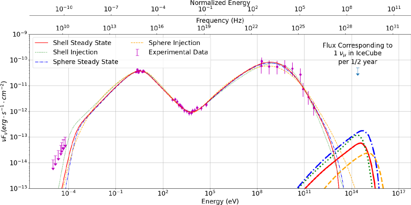
Figure 3: Combined SED for all the models. Thick curves correspond to the predicted neutrino flux.

LABEL:Fig:Combined-SED is a combination of the best SED fits (2) that we can obtain with our model given the parameters that we set a priori. It can be appreciated that all the models can reproduce the SED very well, but they fall short by $\sim 3$ orders of magnitude in the neutrino flux. We return to the neutrino flux in 4.6.

LABEL:Fig:[s]Spherical_Steady_State_Corner, 15, 16 and 17 show the corner plots that we obtain from the MCMC fitting. The blue lines denote the parameters that give the best SED fit.

4.3.1 Spherical Steady State

The spherical steady state model has $9$ parameters: $\left(\gamma_{e,min}\text{, }\gamma_{e,break}\text{, }\gamma_{e,max}\text{, }p_{1}\text{, }p_{2}\text{, }B\text{, }\delta\text{, }R\text{ and }\rho\right)$, but we know from our analysis of 4.1 that some of them are always grouped. Thus, we choose to redefine our parameters in the following way:

$$F_{1} \equiv VN_{1}\delta^{2}\nu_{br}^{2}\gamma_{e,break}^{-p_{1}-1},$$

$$F_{2} \equiv\left(\frac{\gamma_{e,max}}{\gamma_{e,break}}\right)^{3-p_{2}},$$

$$F_{3} \equiv\frac{RN_{1}}{\delta B}\gamma_{e,break}^{-p1},$$

$$\delta \equiv\delta,$$

$$\delta B \equiv\delta B,$$ (97)

$$\nu_{br} \equiv\delta B\gamma_{e,break}^{2},$$

$$\rho \equiv\rho,$$

$$RN_{1} \equiv R\rho\left(p_{1}-1\right)\gamma_{e,min}^{p_{1}-1},$$

$$N_{2} \equiv\gamma_{e,break}^{p_{2}-p_{1}}.$$

As we showed in (LABEL:transform_log_likelihood), we need the Jacobian of the transformation to properly calculate the log-likelihood of the model parameters. This is given by:

$$\left|\frac{dF}{dP}\right| =4\gamma_{e,break}^{2}\left(p_{1}-1\right)\left(p_{2}-3\right).$$ (98)

The best SED that we can achieve is shown in 3 where we can see that it fits quite well to the available data.

The corner plot of the fit can be seen in 14.

Parameter	Spherical Steady State		Disk Steady State		Sphere Injection		Disk Injection
	Best	Median	Best	Median	Best	Median	Best	Median
$\log_{10}\left(\gamma_{e,min}\right)$	$1.33$	$1.96_{-0.65}^{+0.67}$	$1.99$	$2.07_{-0.73}^{+0.60}$	$3.95$	$4.04_{-0.20}^{+0.20}$	$1.47$	$1.73_{-0.51}^{+0.68}$
$\log_{10}\left(\gamma_{e,break}\right)$	$4.03$	$4.10_{-0.24}^{+0.24}$	$4.07$	$4.13_{-0.25}^{+0.23}$	$4.26$	$4.40_{-0.21}^{+0.25}$	$4.39$	$4.31_{-0.24}^{+0.27}$
$\log_{10}\left(\gamma_{e,max}\right)$	$6.82$	$7.89_{-1.48}^{+1.42}$	$6.50$	$7.83_{-1.42}^{+1.47}$	$7.68$	$7.29_{-1.00}^{+1.77}$	$9.01$	$7.99_{-1.38}^{+1.42}$
$p_{1}$	$1.69$	$1.81_{-0.22}^{+0.23}$	$1.71$	$1.83_{-0.23}^{+0.25}$	$1.22$	$1.79_{-0.51}^{+1.00}$	$1.82$	$1.79_{-0.20}^{+0.17}$
$p_{2}$	$4.29$	$4.29_{-0.08}^{+0.10}$	$4.27$	$4.29_{-0.08}^{+0.10}$	$3.37$	$3.43_{-0.12}^{+0.20}$	$3.51$	$3.55_{-0.14}^{+0.23}$
$\log_{10}\left(B\right)$	$-1.01$	$-1.06_{-0.25}^{+0.24}$	$-0.96$	$-1.06_{-0.27}^{+0.27}$	$-1.36$	$-1.38_{-0.16}^{+0.18}$	$-1.09$	$-1.10_{-0.27}^{+0.25}$
$\log_{10}\left(\delta\right)$	$1.43$	$1.37_{-0.37}^{+0.44}$	$1.27$	$1.32_{-0.36}^{+0.44}$	$1.83$	$1.71_{-0.17}^{+0.16}$	$1.04$	$1.22_{-0.35}^{+0.46}$
$\log_{10}\left(h\right)$			$15.93$	$13.49_{-2.14}^{+2.24}$			$13.54$	$13.69_{-0.72}^{+0.78}$
$\log_{10}\left(R\right)$	$16.46$	$16.62_{-0.81}^{+0.80}$	$16.79$	$16.82_{-0.83}^{+0.75}$	$16.12$	$16.43_{-0.53}^{+0.48}$	$17.42$	$17.08_{-0.82}^{+0.65}$
$\log_{10}\left(\rho\right)$	$-21.76$	$-22.29_{-1.03}^{+0.98}$	$-21.71$	$-19.23_{-2.31}^{+2.15}$
$\log_{10}\left(L\right)$					$41.54$	$41.82_{-0.39}^{+0.43}$	$47.46$	$46.37_{-1.87}^{+1.63}$

Table 2: Parameters found for the default fits. The number of points for each model is 309760, 496640, 116480 and 144640 respectively.

4.3.2 Thin Disk Steady State

The thin disk steady state model has $10$ parameters: $\left(\gamma_{e,min}\text{, }\gamma_{e,break}\text{, }\gamma_{e,max}\text{, }p_{1}\text{, }p_{2}\text{, }B\text{, }\delta\text{, }h\text{, }R\text{ and }\rho\right)$. And again, we choose to redefine our parameters in the following way:

$$F_{1} \equiv VN_{1}\delta^{2}\nu_{br}^{2}\gamma_{e,break}^{-p_{1}-1},$$

$$F_{2} \equiv\left(\frac{\gamma_{e,max}}{\gamma_{e,break}}\right)^{3-p_{2}},$$

$$F_{3} \equiv\frac{hN_{1}}{\delta B}\gamma_{e,break}^{-p1},$$

$$\delta \equiv\delta,$$

$$\delta B \equiv\delta B,$$ (99)

$$\nu_{br} \equiv\delta B\gamma_{e,break}^{2},$$

$$\rho \equiv\rho,$$

$$N_{1} \equiv\rho\left(p_{1}-1\right)\gamma_{e,min}^{p_{1}-1},$$

$$hN_{1} \equiv hN_{1},$$

$$N_{2} \equiv\gamma_{e,break}^{p_{2}-p_{1}}.$$

Again, we need the Jacobian of the transformation, which is given by:

$$\left|\frac{dF}{dP}\right| =4\gamma_{e,break}^{2}\left(p_{1}-1\right)\left(p_{2}-3\right).$$ (100)

4.3.3 Spherical Injection

The spherical injection model has $9$ parameters: $\left(\gamma_{e,min}\text{, }\gamma_{e,break}\text{, }\gamma_{e,max}\text{, }p_{1}\text{, }p_{2}\text{, }B\text{, }\delta\text{, }R\text{ and }L\right)$. Unfortunately, due to (LABEL:pop_inj_cooling), the parameter that naturally would take the place of $N_{1}$ in the steady state models depends on the value of $S$, which is not known a priori. Even if it were known, it separates two different behaviours for the particles in two energetic regimes. This makes obtaining simple relations for the synchrotron, x-ray and gamma-ray fluxes a not trivial problem that, although solvable, does not help the fitting. Because of this, we have chosen to not redefine our parameters and fit directly the model parameters.

4.3.4 Thin Disk Injection

The spherical injection model has $10$ parameters: $\left(\gamma_{e,min}\text{, }\gamma_{e,break}\text{, }\gamma_{e,max}\text{, }p_{1}\text{, }p_{2}\text{, }B\text{, }\delta\text{, }h\text{, }R\text{ and }L\right)$. Again, for the same reason as for the case of spherical injection, we choose to not redefine our parameters.

4.4 First Interpretation of Results

First, we check the validity of some of our initial estimates for the initial fitted parameters. For the value of $\log_{10}\left(\delta B\gamma_{e,break}^{2}\right)$ we had estimated $8.50$. LABEL:Fig:Comparison-with-nu_br reflects that, with the exception of the sphere injection model, where we obtain a value $\sim 3$ times bigger, our estimate was correct. A possible explanation for this minor discrepancy lies in (LABEL:pop_inj_cooling). This equation sets the energy which separates the regimes where particles mainly escape from the regime where particles mainly cool. Spherical models have typically higher values of $R$ than discs for $h$, which in turns means higher values for $\tau_{esc}$. Then, everything else being equal, we know that $\gamma_{e,break,sphere}<\gamma_{e,break,disk}$.

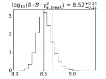
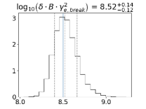
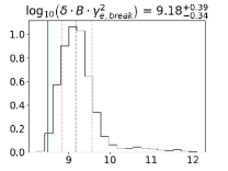
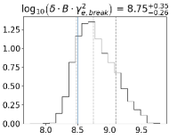
Figure 4: Comparison with the estimates for $\log_{10}\left(\delta B\gamma_{e,break}^{2}\right)$, blue vertical line. From left to right: sphere steady state, disk steady state, sphere injection, disk injection

Second, we check the validity of our initial estimate for $\log_{10}\left(\delta^{2}\frac{V}{\tau_{esc}}\gamma_{e,break}^{-3}\right)$, where we had obtained a value of $35.39$. Note that the factor $V/\tau_{esc}$ depends only on $R^{2}$ regardless of the geometry. LABEL:Fig:Comparison-with-thing shows that we systematically obtain results below the estimate by a factor $\sim 3$. Part of this discrepancy can be explained by looking at the gamma-ray peak of 3. We can see that our model obtains a gamma-ray flux a bit above the data points, although well within the error bars. So, the modelled flux is above that that we used for the estimate, and thus its value should be reduced. The other part comes from the physics used in the estimation, which is based on a crude approximation of inverse Compton upscattering.

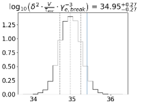
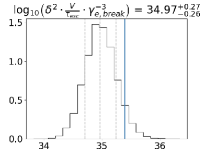
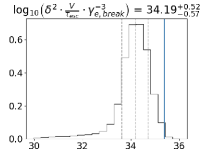
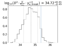
Figure 5: Comparison with the initial estimates for $\log_{10}\left(\delta^{2}\frac{V}{\tau_{esc}}\gamma_{e,break}^{-3}\right)$, blue vertical line. From left to right: sphere steady state, disk steady state, sphere injection, disk injection

Gao et al. (2019) give an estimate for the Eddington luminosity of the black hole at the center of TXS 0506+056 assuming a mass similar to that of M87: $10^{47.8}\,\text{erg}\cdot\text{s}^{-1}$. As one of our parameters for the injection models is precisely injected luminosity, we can directly compare with this value. LABEL:Fig:Comparison-with-L shows that the distribution of values we obtain for spherical injection are well below the estimated one, whereas the values for disk injection are above it.

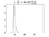
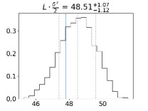
Figure 6: Comparison with Gao et al. (2019)’s estimate for the Eddington luminosity of TXS 0506+056 assuming that the central black hole has a mass similar to that of M87. Left: sphere injection, right: disk injection

The cause for the discrepancy is due to the different behaviour of the particles with low energies in the sphere and disk cases. For the Sphere, the escape timescale is much larger than the cooling timescale, so the high-energy particles have enough time to cool before escaping from the volume and can accumulate, producing a sizable population at low energy. By contrast, the escape timescale for disks are much lower, which allows the low-energy electrons to escape before having enough time to cool.

This is confirmed by the steady-state models that show the need for a low-energy population of electrons through their low values for $\gamma_{e,min}$ ($\log_{10}$ of $1.96$ for the sphere steady-state model, versus $4.04$ for injection). As mentioned above, although the sphere injection model can obtain a low-energy population through cooling, the disk injection model needs to include this in the injection directly ($\log_{10}\gamma_{e,min}$ of $1.73$ for disk injection, versus the aforementioned $4.04$ for disk injection).

From the results of the spherical steady state model, we can integrate the amount of particles between $\gamma_{e,min}$ and $\gamma_{e,break}$ to find that about $98\%$ of the electrons are in this range of energies. By using (LABEL:L_related_with_rho) we can calculate an rough estimate of the luminosity that would be required to obtain a population of electrons similar to that of the steady state case in a pure injection and escape case, obtaining a value of $L_{estimated}\sim 10^{46}$, which is in line with the estimate for the Eddington Luminosity (after a frame transformation).

4.5 Interpretation of Posterior Distribution Results and Cross-Correlations

As discussed in 3 when we presented the procedure of fitting with MCMC, one of the products that we obtain is the posterior density function for each of the parameters. And that, in turn, can provide interesting information, for example about how individual parameters impact a model or whether or not bimodalities occur across the range of good fits. One example of the former are the posterior density functions for $\gamma_{e,max}$. We have not found examples of bimodal distributions.

The four $\gamma_{e,max}$ posterior distributions clearly show a lower cut off at low energies and a flat shape at the rest of the energies in the explored parameter space. The lower cut-off can be explained by the constraints of (LABEL:[)s]gamma_max_constraint and (57), whereas the flat shape can be explained by realizing that our model is not constraining at this range. In fact, an increase of $\gamma_{e,max}$ requires a number of particles so small that it can barely modify $\rho$ or $L$.

Another of the products of using MCMC are the correlation plots between the parameters, where we can clearly see the relations between the parameters and how changing one affects others. Good examples are the triad $\gamma_{e,break}\text{, }\delta\text{, }R$ or the correlation between $\rho$ and $R$ or $h$ depending on the geometry of the emitting volume for steady state models.

The correlations between $\gamma_{e,break}\text{, }\delta\text{ and }R$ can be explained by (LABEL:delta_g_break_R). $V/\tau_{esc}$ is a function of $R^{2}$ regardless of the geometry of the model, which is the cause of the cross-correlations.

The correlation between $\rho$ and $R$ or $h$ involves the escape timescale $\tau_{esc}$. As stated in the previous paragraph, $V/\tau_{esc}$ is only a function of $R^{2}$, which means that when transforming from the number of photons in the blob to the received flux the only geometric factor is $R^{2}$. But, from our exploration of both synchrotron emission and inverse Compton emission, we found that the population of photons in the rest frame of the fluid depends on $\tau_{esc}$. This means that the population depends directly on $R$ or $h$ depending on whether the geometry is a sphere or a disk.

For a posterior distribution of $h$ peaking around $10^{13}$ cm, we note that the thin disk model is in tension with the assumption that the plasma is able to contain the upper high-energy part at $\gamma\sim 10^{6}$ of a population of protons. At magnetic fields $B$ of $0.1$ G, their gyroradius becomes of an order comparable to $h$, leaving little room for diffusion (accounted for through our $\sigma$ parameter). Sphere models are therefore arguably preferable to disk models for explaining a high-energy proton population responsible for a measurable neutrino flux.

A more detailed analysis of the posterior density functions for the case of the spherical injection model reveals something interesting. In the case of the distribution for $p_{1}$, we find that its distribution is much more extended than the ones for the other three models. Moreover, looking at the distributions for $\gamma_{e,min}$ and $\gamma_{e,break}$ we find that their ranges overlap and, as can be seen in 7, if we plot the distribution for both combined we find that we obtain a single peak. We infer that the first part of the broken power law is not relevant for the fit, as it is very narrow and its slope can vary wildly.

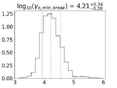
Figure 7: Probability density function for $\gamma_{e,min}$ and $\gamma_{e,break}$ together for the Spherical Injection model

To check the validity of this reasoning. We have chosen to also test the case of the spherical injection but with a simple power law.

4.5.1 Spherical Injection with a Power Law

The spherical injection with a power law model has $7$ parameters: $\left(\gamma_{e,min}\text{, }\gamma_{e,max}\text{, }p\text{, }B\text{, }\delta\text{, }R\text{ and }L\right)$ where we again have chosen to not redefine them.

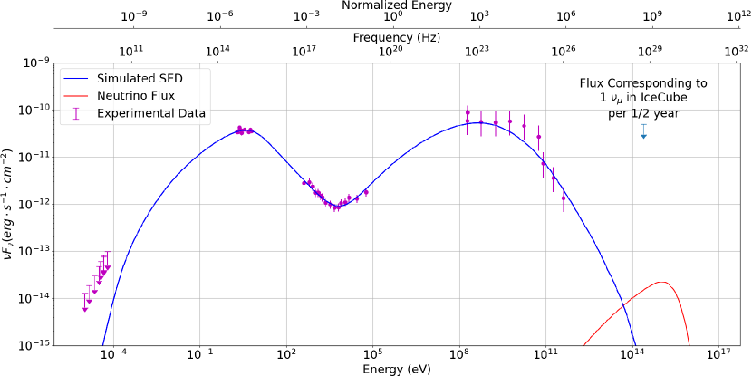
Figure 8: SED resulting from the best parameters for the Sphere Injection with a Power Law.

Parameter	Spherical Injection		Spherical Injection		Spherical Injection
			Simple Power Law		Simple Power Law varying $\eta$
	Best	Median	Best	Median	Best	Median
$\log_{10}\left(\gamma_{e,min}\right)$	$3.95$	$4.04_{-0.20}^{+0.20}$	$4.04$	$4.12_{-0.22}^{+0.21}$	$4.03$	$4.04_{-0.19}^{+0.19}$
$\log_{10}\left(\gamma_{e,break}\right)$	$4.26$	$4.40_{-0.21}^{+0.25}$
$\log_{10}\left(\gamma_{e.max}\right)$	$7.68$	$7.29_{-1.00}^{+1.77}$	$7.31$	$7.83_{-1.37}^{+1.43}$	$7.53$	$7.69_{-1.51}^{+1.55}$
$p_{1}$	$1.22$	$1.79_{-0.51}^{+1.00}$
$p_{2}$	$3.37$	$3.43_{-0.12}^{+0.20}$	$3.31$	$3.35_{-0.10}^{+0.14}$	$3.37$	$3.40_{-0.11}^{+0.18}$
$\log_{10}\left(B\right)$	$-1.36$	$-1.38_{-0.16}^{+0.18}$	$-1.32$	$-1.36_{-0.19}^{+0.20}$	$-1.33$	$-1.30_{-0.20}^{+0.19}$
$\log_{10}\left(\delta\right)$	$1.83$	$1.71_{-0.17}^{+0.16}$	$1.82$	$1.74_{-0.22}^{+0.21}$	$1.85$	$1.85_{-0.17}^{+0.16}$
$\log_{10}\left(R\right)$	$16.12$	$16.43_{-0.53}^{+0.48}$	$16.09$	$16.32_{-0.66}^{+0.65}$	$16.03$	$16.00_{-0.53}^{+0.55}$
$\log_{10}\left(\eta\right)$					$3.53$	$3.48_{-0.28}^{+0.26}$
$\log_{10}\left(L\right)$	$41.54$	$41.82_{-0.39}^{+0.43}$	$41.53$	$41.75_{-0.50}^{+0.58}$	$44.97$	$44.91_{-0.61}^{+0.64}$

Table 3: Parameters of the Sphere Injection with a Power Law Model and a the same case allowing the ratio of injected protons to electrons $\left(\eta\right)$ to change, with 234240 and 168960 points, respectively. The leftmost spherical injection columns repeat the base case of Spherical Injection for comparison purposes.

LABEL:Tab:Spherical_Injection_variations_Parameters (central two columns) corresponds to the parameter values that we have found, 8 shows the SED corresponding to the best parameters, and 18 shows the corresponding corner plot of the model.

As we can see in 8, the fit that we obtain is very similar to that of the broken power law model. We conclude that a simple power law is indeed sufficient to reproduce the observed SED for an injection model in spherical geometry.

4.6 Large proton to electron ratio injection

LABEL:Fig:Combined-SED shows the comparison between the SED we obtained with the four models and the observed fluxes. For $\eta=1$ (equal injection numbers for protons and electrons), the SED can be produced very well, but the neutrino flux remains orders of magnitude below that allowed by the tentative neutrino detection. Below we discuss two mechanisms to increase the neutrino flux.

One option is to shift the value of gamma_p,max. As discussed in 4.3, a value of $10^{6}$ is enough to produce neutrinos with the appropriate energy through more than one channel. Nevertheless, higher energies allow for a greater energy range for protons, pions and muons to produce neutrinos with $\sim 290$ TeV. Additionally, an increase of the maximum energy for protons also increases the total number of protons that have energies above the threshold to produce neutrinos at $290$ TeV, thus leading to an increase of the total neutrino flux. For example Keivani et al. (2018) uses $\gamma_{p,max}=1.6\times 10^{6}-3\times 10^{9}$ and Cerruti et al. (2018) has $\gamma_{p,max}=6\times 10^{7}-2.5\times 10^{9}$.

The second option is to increase the ratio of protons to electrons, both in the steady state population and in the injected population. The main consequence that a higher value of $\eta$ would have is an increase of the number of protons at all energies, including those with the appropriate one to produce neutrinos. Thus, we will obtain a higher neutrino flux at all energies. For example Gao et al. (2019) uses $\eta\approx 8606$ (as we show in Appendix B) and Cerruti et al. (2018) has $\eta\approx 200$ Appendix A.

LABEL:Fig:Combined-Neutrino-tests shows a simple test of these two hypotheses with our model. As a base we have taken the best parameters for the spherical injection model. Then, to check the first hypothesis we have increased the value of $\gamma_{p,max}$ to $10^{9}$ and to check the second we have increased the value of $\eta$ by a factor 1750 and modified the value of $L$ according to (LABEL:Q_from_L) so that the value of injected electrons is the same in the two models. As we predicted in the previous paragraphs, in the first case we see an increase in the total flux of neutrinos, specially those with energies higher than $500$ TeV, whereas in the second case the increase is restricted only to those of energies around $290$ TeV.

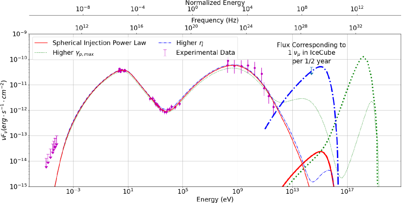
Figure 9: Combined neutrino tests. The red line corresponds to the reference of the best result for the spherical injection with a simple power law model, the green dots correspond to the same model but increasing $\gamma_{p,max}$ to $10^{9}$ and the blue dot dashed line corresponds to the same model but increasing $\eta$ by $1750$. Thick lines correspond to the predicted neutrino flux.

Following 9, and combined with the simplicity of the spherical injection with a single power law model, we choose to go further in our modelling and allow the value of $\eta$ to vary. The neutrino flux is an upper limit, so we do not have an actual data point to compare our model results, but for illustrative purposes, we have chosen to act as if the upper limit was an actual detection and use its value in the calculation of the log-likelihood.

The model that we fit has 8 parameters: $\left(\gamma_{e,min}\text{, }\gamma_{e,max}\text{, }p\text{, }B\text{, }\delta\text{, }R\text{, }\eta\text{ and }L\right)$

LABEL:Tab:Spherical_Injection_variations_Parameters (two rightmost columns) corresponds to the parameter values that we have found, 10 shows the fit that we obtain with the best parameters and 19 shows the corresponding corner plot of the model. LABEL:Fig:eta_histogram plots the resulting probability density function for $\eta$, showing a broad distribution peaking around $\log_{10}\eta=3.48$. Below $\eta$ of $\sim 10^{3}$, the neutrino flux will be underpredicted, whereas for eta approaching $10^{4}$ it becomes difficult to avoid overpredicting the X-ray flux in the SED valley.

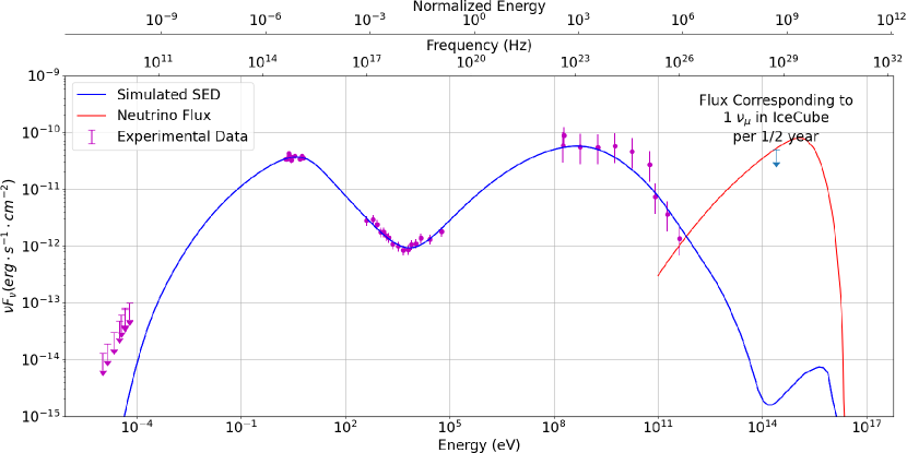
Figure 10: SED for the best parameters of the Spherical Injection with a Power Law allowing $\eta$ to vary.

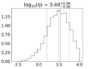
Figure 11: Probability density function for $\eta$.

It can be seen from 10 that both the SED and the neutrino flux can be fitted at the same time without overwhelming the x-ray flux. But the best-fitting curve in the figure uses $\eta\approx 3388$ (i.e. the value indicated by a blue line in 11) for the ratio of protons to electrons, which implies a discrepancy of orders of magnitude in the numbers of accelerated protons and electrons injected in the plasma.

5 Summary and Conclusions

We present a detailed kinetic lepto-hadronic emission model capable of producing photon and neutrino spectra for a range of parameters, plasma geometries and electrons and protons either injected or at steady state. This model has been developed independently of other approaches (e.g. Cerruti et al. (2015) or Gao et al. (2017)), and can be used as a cross-check on their work. We have coupled our model to a Markov-Chain Monte Carlo method, and discuss the characteristics of the parameter space that this allows us to probe in a novel manner. The method is applied to the multi-messenger case of TXS 0506+056.

MCMC sampling reveals the full probability distribution of the fit parameters as well as their cross-correlations and degeneracies. We demonstrate that the six iterations of our model (between sphere and disk geometry, steady state and injection, simple power-law and varying $\eta$) are all able to fit TXS 0506+056. The MCMC method shows that a single power law injection of electrons is sufficient in spherical geometry, that $\gamma_{e,max}$ is poorly constrained and that some of the fitted variables are correlated.

To reproduce a high level of neutrino flux comparable to the peak value allowed by the tentative detection by IceCube requires a large proton to electron ratio. Our MCMC method quantifies the probability distribution of this ratio eta, and we find $\log_{10}\eta=3.48_{-0.28}^{+0.26}$. If the accelerated protons and electrons are not taken to be from different origins altogether, this poses a challenge to models of charged particle acceleration to explain the origin of an overwhelmingly larger number of accelerated protons than electrons.

Data availability

The observational data used in this paper was taken from IceCube et al. (2018). All data produced in this analysis is available upon request. The software used in this study is available upon request, but will be made open-source in the near future (Jimenez-Fernandez & van Eerten, in prep).

Appendix A Notes on reproducing the work of Cerruti et al.

As a way of checking our model, we try to reproduce the results of Cerruti et al. (2018). Their study has both hadronic and lepto-hadronic models and their parameters and the goodness of the fit are available in the extra materials. We choose to reproduce the parameters for a lepto hadronic model that give the best $\chi^{2}$ value.

Cerruti et al.’s model is based upon a stationary particle distribution with the shape of a broken power-law with an exponential drop which produces the primary photon emission. Although for this work, they set $\gamma_{e,break}=\gamma_{e,max}$, obtaining a simple power law. In addition, they calculate the lepton population that would result from photon-photon pair production and bethe-heitler cascades and subsequently add their own emission to the primary emission. For the neutrino emission, they calculate the resulting emission from pion and muon decays.

This hybrid approach to the calculation of the lepton population poses a problem for our model as we can either have a single steady state population or a fully dynamic one. Moreover, as we will see when we derive the corresponding parameters for our model, these can easily cause that one of our assumptions, that of the lepton injection due to pair production and bethe-heitler processes being small, to be broken. With this in mind, we choose to employ the spherical steady state version of our model, knowing that it will not be able to fully reproduce the shape of the observed SED.

As said, their model defines the steady populations for electrons and protons as:

$$N_{e,p}\left(\gamma\right)=K_{e,p}^{\prime}\gamma^{-\alpha_{e,p}}\exp\left(-\frac{\gamma}{\gamma_{e,p,max}}\right).$$ (101)

Their population parameter $K_{e,p}^{\prime}$ is given in term of the normalizations for the electron distribution at $\gamma=1$ and the ratio with protons $\left(r\right)$. This means that:

$$N_{e}\left(1\right)=K_{e} =K_{e}^{\prime}\exp\left(-\frac{1}{\gamma_{e,max}}\right),$$ (102)

$$N_{p}\left(1\right)=K_{p} =rK_{e}.$$ (103)

So:

$$K_{e}^{\prime} =\phantom{r}K_{e}\exp\left(\frac{1}{\gamma_{e,max}}\right),$$ (104)

$$K_{p}^{\prime} =rK_{e}\exp\left(\frac{1}{\gamma_{p,max}}\right).$$ (105)

Our model defines the population parameters differently but we can transform between the two as:

$$\frac{\rho}{m_{e}+\eta m_{p}}A =\phantom{r}K_{e}\exp\left(\frac{1}{\gamma_{e,max}}\right),$$ (106)

$$\frac{\eta\rho}{m_{e}+\eta m_{p}}C =rK_{e}\exp\left(\frac{1}{\gamma_{p,max}}\right).$$ (107)

So:

$$\eta =\frac{A}{C}r\frac{\exp\left(\frac{1}{\gamma_{p,max}}\right)}{\exp\left(\frac{1}{\gamma_{e,max}}\right)},$$ (108)

$$\rho =\frac{K_{e}}{A}\exp\left(\frac{1}{\gamma_{e,max}}\right)\left(m_{e}+\eta m_{p}\right),$$ (109)

where $A$ and $C$ are normalization constants for the particles distributions.

LABEL:Tab:cerruti_our_parameters shows the results of the translation of the parameters between Cerruti et al.’s model and ours. There are three parameters that will have a very marked effect on the resulting SED: $\gamma_{e,max}$, $\gamma_{p,max}$ and $\eta$. The first $\left(\gamma_{e,max}\right)$ effectively sets the maximum energy of synchrotron and Inverse Compton photons, and as it is two orders of magnitude lower than ours, we can predict that we will not be able to fit neither the high energy end of the synchrotron peak, nor that of the Inverse Compton peak. The second $\left(\gamma_{p,max}\right)$ contributes to increasing the amount of protons available to interact with photons in both, pion production and bethe-heitler pair production. This will cause the amount of injected leptons and neutrinos to increase, and their energies will be bigger. The third $\left(\eta\right)$ has a similar effect to $\gamma_{p,max}$, but increases the number of protons at all energies. This means that not only the pion and lepton production will be higher, but also the synchrotron emission.

Parameter	Description	Cerruti	Ours
$B$	Magnetic Field $\left(G\right)$	$0.376356$	$0.376356$
$R$	Blob Radius $\left(cm\right)$	$4.2638\times 10^{15}$	$4.2638\times 10^{15}$
$\delta$	Doppler Factor	$40$	$40$
$\alpha_{e}$	$e^{-}$ spectral index	$2$	$2$
$\gamma_{e,min}$	Minimal $e^{-}$ Lorentz factor	$500$	$500$
$\gamma_{e,max}$	Maximal $e^{-}$ Lorentz factor	$10926.6$	$10926.6$
$\alpha_{p}$	$p^{+}$ spectral index	$2$	$2$
$\gamma_{p,min}$	Minimal $p^{+}$ Lorentz factor	$1$	$1$
$\gamma_{p,max}$	Maximal $p^{+}$ Lorentz factor	$1.02547\times 10^{8}$	$1.02547\times 10^{8}$
$K_{e}$	Normalization constant	$60659.7$	-
$K_{p}/K_{e}$	Ratio of the normalization	$0.381661$	-
$\rho$	Density	-	$3.872355422482072\times 10^{-20}$
$\eta$	$p^{+}$ to $e^{-}$ ratio	-	$200$

Table 4: List of parameters for reproducing the SED of TXS 0506+056 by Cerruti et al. and the adaptation to our model.

LABEL:Fig:Cerruti_reproduction shows the results obtained by our model using Cerruti et al.’s parameters. We have chosen to separate the simulated SED in the total range and a trusted range because, as we have explained, we can not be sure of the emission that would come from electrons with energies above that of injection. Still, for the trusted range, we obtain an acceptable fit with the observed flux levels. Although the neutrino flux is still lower than the estimated by Ice Cube at the relevant energies.

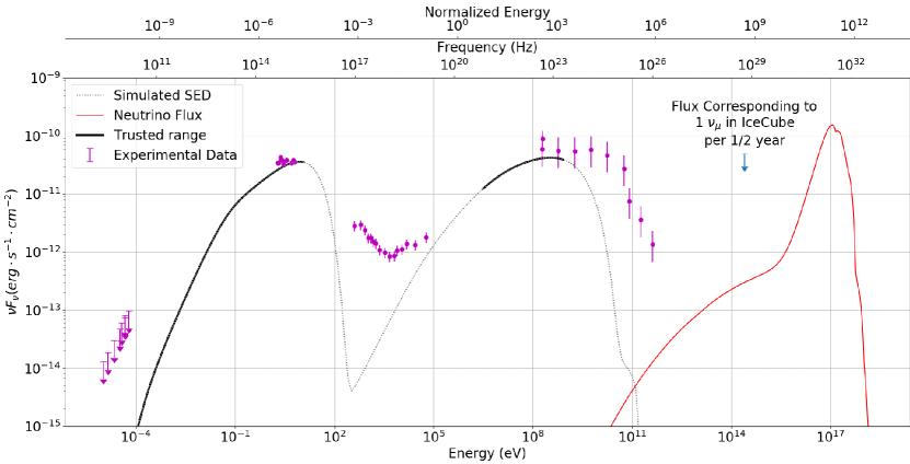
Figure 12: SED and neutrino flux obtained with the parameters from Cerruti et al. (2018)

Appendix B Notes on reproducing the work of Gao et al.

A second check that we can do for our model is to try to reproduce the SED of TXS 0506+056 employing the parameters of the lepto-hadronic model of Gao et al.’s hybrid model. It must be noted that in their model, they separate the luminosities of protons and electrons, whereas in our model we combine them into one luminosity and regulate the particle populations by means of the ratio of protons to electrons parameter.

In their model:

$$L_{e,p}=m_{e,p}c^{2}\times\int\gamma K_{e,p}\gamma^{-\alpha_{e,p}}d\gamma.$$ (110)

By separating $K_{e,p}\gamma^{-\alpha_{e,p}}$into a normalized distribution and a constant, as we did in 2.4 we easily find:

$$Q_{e,p,0}=\frac{L_{e,p}}{\left\langle\gamma_{e,p}\right\rangle m_{e,p}c^{2}}.$$ (111)

The ratio of injected protons to electrons is then:

$$\eta=\frac{Q_{p,0}}{Q_{e,0}}=\frac{L_{p}}{\left\langle\gamma_{p}\right\rangle}\frac{\left\langle\gamma_{e}\right\rangle}{L_{e}}\frac{m_{e}}{m_{p}}.$$ (112)

Using the parameters of Gao et al. (Gao et al., 2019) we obtain $\eta=8606$.

Another difference between our model and theirs is that they take that the charged particles do not escape in the free escape timescale, as they assume that protons, electrons and positrons escape with a velocity of $c/300$. We have chosen to simulate this by setting $\sigma=300$ which has the same effect. Another difference lies in the definition of the free escape timescales, where we have included a factor $3/4$ due to geometrical reasons (2):

$$t_{esc,our}=\frac{3}{4}t_{esc,gao}.$$ (113)

In 5 we list the original parameters and our choices.

Parameter	Description	Gao	Ours
$B$	Magnetic Field $\left(G\right)$	$0.14$	$0.14$
$R$	Blob Radius $\left(cm\right)$	$10^{16}$	$10^{16}$
$\delta$	Doppler Factor	$28.0$	$28.0$
$L_{e}$	$e^{-}$ injection luminosity $\left(erg/s\right)$	$10^{40.9}$	-
$\alpha_{e}$	$e^{-}$ spectral index	$-3.5$	$-3.5$
$\gamma_{e,min}$	Minimal $e^{-}$ Lorentz factor	$10^{4.2}$	$10^{4.2}$
$\gamma_{e,max}$	Maximal $e^{-}$ Lorentz factor	$10^{5.1}$	$10^{5.1}$
$L_{p}$	$p^{+}$ injection luminosity $\left(erg/s\right)$	$10^{45.7}$	-
$\alpha_{p}$	$p^{+}$ spectral index	$-2.0$	$-2.0$
$\gamma_{p,min}$	Minimal $p^{+}$ Lorentz factor	$10.0$	$10.0$
$\gamma_{p,max}$	Maximal $p^{+}$ Lorentz factor	$10^{5.4}$	$10^{5.4}$
$L$	Injection luminosity $\left(erg/s\right)$	-	$10^{45.7}$
$\eta$	$p^{+}$ to $e^{-}$ ratio	-	$8606$
$\eta_{esc}$	escape velocity of $e^{\pm}$ and $p^{+}$	$c/300$	$c/300$

Table 5: List of parameters for reproducing the SED of TXS 0506+056 by Gao et al and the adaptation to our model. It should be noted that both injections are taken as being a simple power law and the volume a sphere.

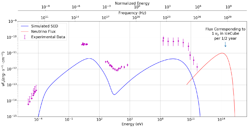
Figure 13: SED and neutrino flux obtained with the parameters from Gao et al. (2019)

13 shows the resulting SED and neutrino flux that we obtain applying our model with the parameters of (Gao et al., 2019). It is clear that, although the shape is correct, we are not able to correctly reproduce the flux level, being our prediction lower by $\sim 1$ order of magnitude. It should be noted that their model is, in effect, a two zone model, consisting of two concentric spheres, and that we are modelling the emission of the inner sphere for the purpose of our comparison. Our analysis of the injection terms for electrons and positrons from the Bethe-Heitler process suggests that the photon field is not sufficient to produce the amount of high-energy electrons needed to give rise to the required gamma-ray flux. The main hypothesis that we have is that the external sphere that the model of Gao et al include injects enough low energy photons to the inner sphere to trigger a pair cascade, and that subsequently, these high-energy pairs are responsible for the upscattering of photons up to gamma-ray energies.

Appendix C Corner Plots

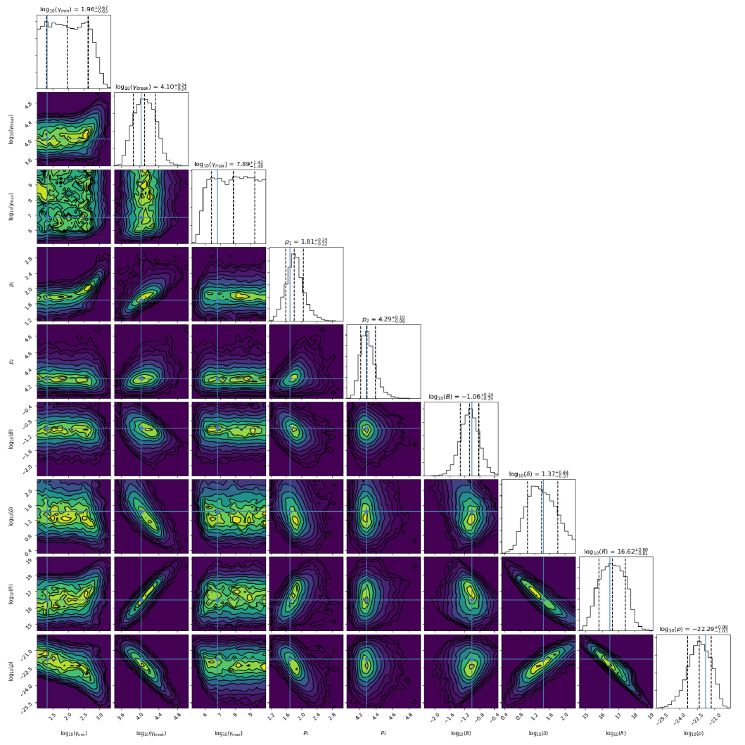
Figure 14: Corner plot of the fit to the Sphere Steady State Model

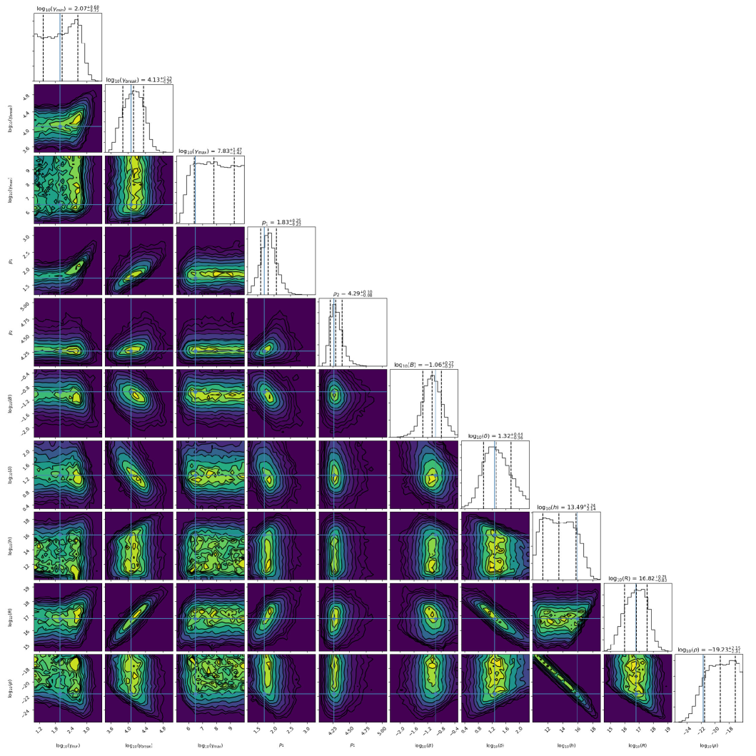
Figure 15: Corner plot of the fit to the Disk Steady State Model

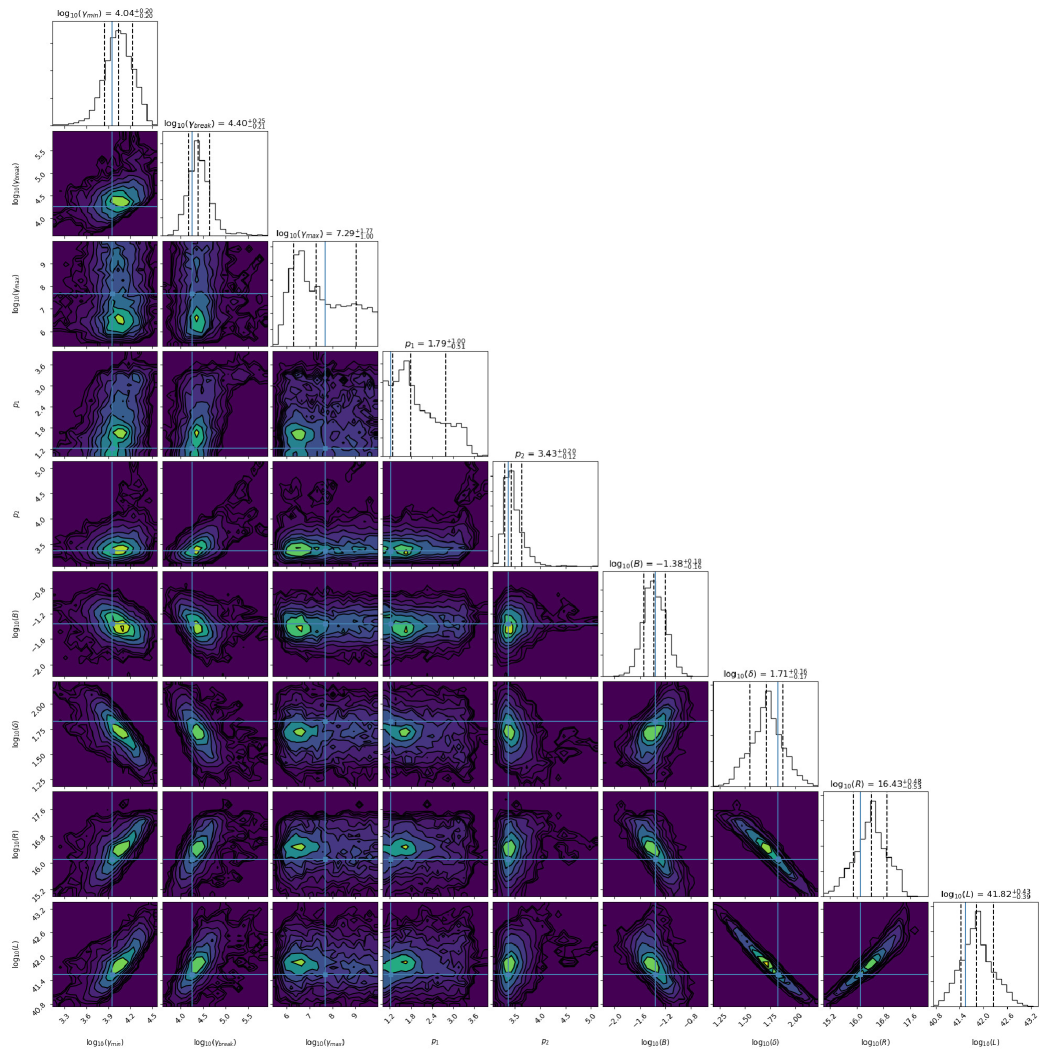
Figure 16: Corner plot of the fit to the Sphere Injection Model

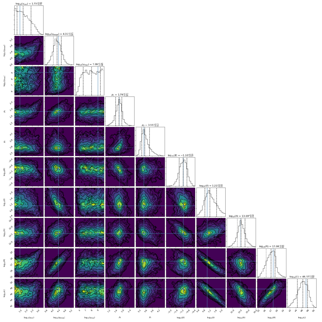
Figure 17: Corner plot of the fit to the Disk Injection Model

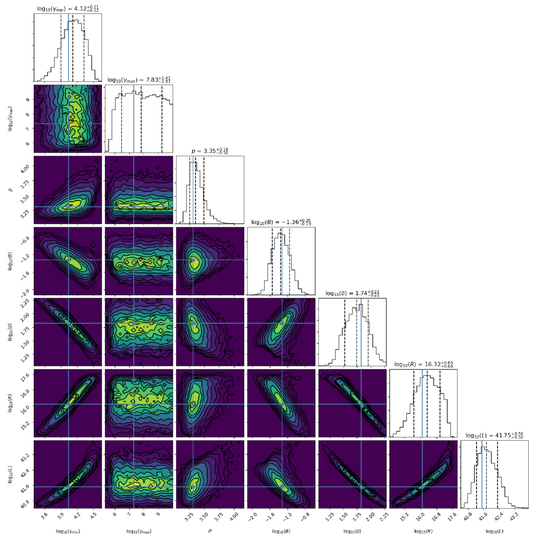
Figure 18: Corner plot of the fit to the Sphere Injection with a Power Law Model

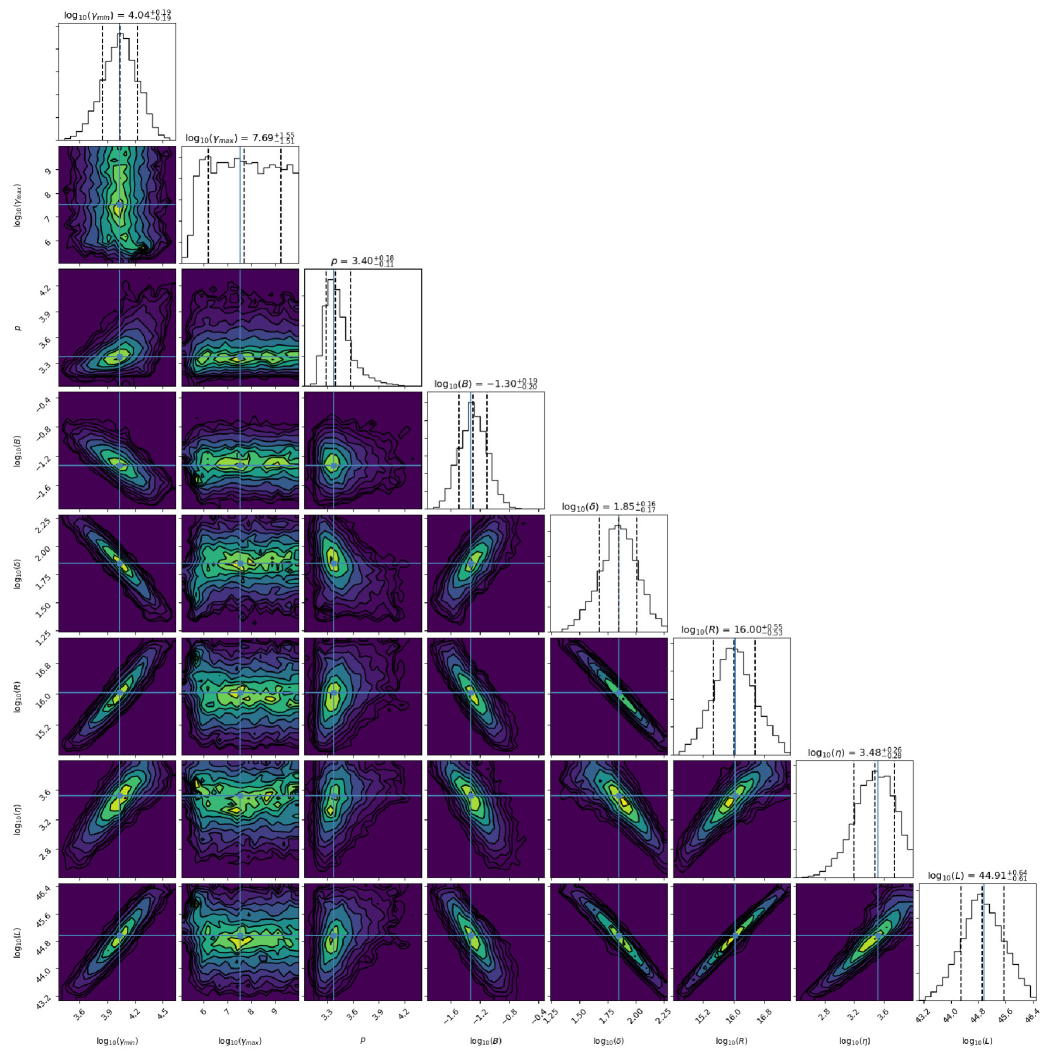
Figure 19: Corner plot of the fit to the Sphere Injection with a Power Law Model allowing $\eta$ to vary.

References

- Böttcher (2019) Böttcher M., 2019, arXiv:1901.04178 [astro-ph]
- Böttcher & Baring (2019) Böttcher M., Baring M. G., 2019, arXiv:1903.12381 [astro-ph]
- Böttcher & Dermer (2010) Böttcher M., Dermer C. D., 2010, The Astrophysical Journal, 711, 445
- Böttcher & Schlickeiser (1997) Böttcher M., Schlickeiser R., 1997, Astronomy & Astrophysics, p. 5
- Böttcher et al. (2012) Böttcher M., Harris D. E., Krawczynski H., 2012, Relativistic Jets from Active Galactic Nuclei
- Böttcher et al. (2013) Böttcher M., Reimer A., Sweeney K., Prakash A., 2013, The Astrophysical Journal, 768, 54
- Cerruti et al. (2015) Cerruti M., Zech A., Boisson C., Inoue S., 2015, Monthly Notices of the Royal Astronomical Society, 448, 910
- Cerruti et al. (2018) Cerruti M., Zech A., Boisson C., Emery G., Inoue S., Lenain J.-P., 2018, preprint, (arXiv:1807.04335)
- Collaboration et al. (2019) Collaboration P., et al., 2019, arXiv:1807.06209 [astro-ph]
- Crusius & Schlickeiser (1986) Crusius A., Schlickeiser R., 1986, Astronomy & Astrophysics, 164, L16
- Foreman-Mackey et al. (2013) Foreman-Mackey D., Hogg D. W., Lang D., Goodman J., 2013, Publications of the Astronomical Society of the Pacific, 125, 306
- Gao et al. (2017) Gao S., Pohl M., Winter W., 2017, The Astrophysical Journal, 843, 109
- Gao et al. (2019) Gao S., Fedynitch A., Winter W., Pohl M., 2019, Nature Astronomy, 3, 88
- Goodman & Weare (2010) Goodman J., Weare J., 2010, Communications in Applied Mathematics and Computational Science, 5, 65
- Graff et al. (2008) Graff P. B., Georganopoulos M., Perlman E. S., Kazanas D., 2008, The Astrophysical Journal, 689, 68
- Hümmer et al. (2010) Hümmer S., Rüger M., Spanier F., Winter W., 2010, The Astrophysical Journal, 721, 630
- IceCube et al. (2018) IceCube T., et al., 2018, Science, 361
- Jones (1968) Jones F. C., 1968, Physical Review, 167, 1159
- Keivani et al. (2018) Keivani A., et al., 2018, The Astrophysical Journal, 864, 84
- Kelner & Aharonian (2008) Kelner S. R., Aharonian F. A., 2008, Physical Review D, 78
- Kino et al. (2004) Kino M., Mizuta A., Yamada S., 2004, The Astrophysical Journal, 611, 1021
- Lipari et al. (2007) Lipari P., Lusignoli M., Meloni D., 2007, Physical Review D, 75
- Liu et al. (2018) Liu R.-Y., Wang K., Xue R., Taylor A. M., Wang X.-Y., Li Z., Yan H., 2018, arXiv:1807.05113 [astro-ph]
- MacDonald et al. (2015) MacDonald N. R., Marscher A. P., Jorstad S. G., Joshi M., 2015, The Astrophysical Journal, 804, 111
- Mastichiadis & Kirk (1995) Mastichiadis A., Kirk J. G., 1995, Astronomy & Astrophysics, 295, 613
- Mastichiadis et al. (2005) Mastichiadis A., Protheroe R. J., Kirk J. G., 2005, Astronomy & Astrophysics, 433, 765
- Morris et al. (2019) Morris P. J., Potter W. J., Cotter G., 2019, Monthly Notices of the Royal Astronomical Society, 486, 1548
- Murase et al. (2018) Murase K., Oikonomou F., Petropoulou M., 2018, The Astrophysical Journal, 865, 124
- Pe’er et al. (2017) Pe’er A., Long K., Casella P., 2017, The Astrophysical Journal, 846, 54
- Petropoulou & Mastichiadis (2015) Petropoulou M., Mastichiadis A., 2015, Monthly Notices of the Royal Astronomical Society, 447, 36
- Petropoulou et al. (2019) Petropoulou M., Sironi L., Spitkovsky A., Giannios D., 2019, arXiv:1906.03297 [astro-ph]
- Potter (2018) Potter W. J., 2018, Monthly Notices of the Royal Astronomical Society, 473, 4107
- Qin et al. (2018) Qin L., Wang J., Yang C., Yuan Z., Kang S., Mao J., 2018, Publications of the Astronomical Society of Japan, 70
- Spada et al. (2001) Spada M., Ghisellini G., Lazzati D., Celotti A., 2001, Monthly Notices of the Royal Astronomical Society, 325, 1559
- Svensson (1982) Svensson R., 1982, The Astrophysical Journal, 258, 321
- Xue et al. (2019) Xue R., Liu R.-Y., Petropoulou M., Oikonomou F., Wang Z.-R., Wang K., Wang X.-Y., 2019, arXiv:1908.10190 [astro-ph]