Optimal elasticity of biological networks

Abstract

Reinforced elastic sheets surround us in daily life, from concrete shell buildings to biological structures such as the arthropod exoskeleton or the venation network of dicotyledonous plant leaves. Natural structures are often highly optimized through evolution and natural selection, leading to the biologically and practically relevant problem of understanding and applying the principles of their design. Inspired by the hierarchically organized scaffolding networks found in plant leaves, here we model networks of bending beams that capture the discrete and non-uniform nature of natural materials. Using the principle of maximal rigidity under natural resource constraints, we show that optimal discrete beam networks reproduce the structural features of real leaf venation. Thus, in addition to its ability to efficiently transport water and nutrients, the venation network also optimizes leaf rigidity using the same hierarchical reticulated network topology. We study the phase space of optimal mechanical networks, providing concrete guidelines for the construction of elastic structures. We implement these natural design rules by fabricating efficient, biologically inspired metamaterials.

Elastic sheets reinforced by beams are pervasive in nature and engineering. From concrete shell buildings Melaragno (2012) to aircraft fuselages Niu and Niu (1999), reinforced shells have found numerous applications due to their rigidity and efficient use of resources. Evolution and natural selection have also produced structures such as plant leaves, which need to remain flat to maximize photosynthesis Niklas (1992, 1999); Roth-Nebelsick et al. (2001); Sack and Scoffoni (2013), or dragonfly wings, which combine light weight and rigidity to enable efficient flight Sun and Bhushan (2012). Uncovering the design rules behind biologically optimized natural materials may not just impact engineering but also illuminate their role in evolution.

Efficient design of thin shells is an active research problem Gil-Ureta et al. (2019); Sakai et al. (2020); Seranaj et al. (2018); Townsend and Kim (2019); Bendsøe and Sigmund (2003); Ramm et al. (1993); Hassani et al. (2013), and mechanical metamaterials have emerged as promising candidates for efficient, rigid and tunable structures Bertoldi et al. (2017); Overvelde et al. (2017); Gross et al. (2019); Goodrich et al. (2015); Ronellenfitsch et al. (2019); Gurtner and Durand (2014). Natural materials are often characterized by a fractal-like hierarchical organization. Specifically, the venation of plant leaves is known to play a crucial role in the transport of water and nutrients Katifori (2018), and in the structural rigidity of the lamina Sack and Scoffoni (2013); Roth-Nebelsick et al. (2001); Niklas (1992), so as to allow the plant to maximize area for photosynthesis while being compliant with the wind and other forces Ennos (2005); Vogel (2012). While much work has been done to characterize the venation networks of dicotyledonous plants in terms of geometry Wright et al. (2004); Blonder et al. (2011); Kull and Herbig (1994), topology Katifori and Magnasco (2012); Mileyko et al. (2012); Ronellenfitsch et al. (2015), and optimal fluid transport Katifori et al. (2010a); Corson (2010); Hu and Cai (2013); Ronellenfitsch and Katifori (2016, 2019); Gavrilchenko and Katifori (2019), the mechanical purpose, properties, and optimality of the venation network beyond the midrib Niklas (1992); Gilet and Bourouiba (2015); Niklas (1999); Wei et al. (2012) have received less attention Sun et al. (2018). Recent work points towards the importance of mechanical traits Blonder et al. (2020).

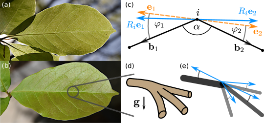
Figure 1: Leaf venation as a discrete beam network. (a) Abaxial surface of a leaf of Magnolia sp., showing the hierarchically organized reticulate venation network keeping the lamina flat and rigid, and transporting water and nutrients. (b) Adaxial surface of the same leaf, emphasizing the venation network embedded in the lamina. (c) Discretized model of beam bending. Dashed orange arrows correspond to the local reference frame $\{\mathbf{e}_{1,2}\}$ used to construct the elastic energy Eq. (2) with $\sin^{2}\varphi_{1,2}=\|\mathbf{e}_{1,2}\times\mathbf{b}_{1,2}\|^{2}$. The reference frame $\{R_{i}\,\mathbf{e}_{1,2}\}$ compensating overall rigid rotations is shown in blue. (d) Plant leaf venation subject to gravitational load $\mathbf{g}$ as prototypical example of a natural DBN. One large vein branches off into three smaller veins that all bend under the load. (e) DBN model of the node from (d). Each discrete beam joining at the node is depicted with its bending constant by line thickness and color. Deviations from the local reference (blue) are penalized by Eq. (3).

Here, we ask to which extent leaves and similar natural materials may be mechanically optimized, what rules their natural design underlies, and how these rules can be applied.

To answer these questions, we consider a model of discrete beam networks (DBNs) to capture the properties of natural materials. Specifically, DBNs model bending beams with arbitrary stiffness that are joined to form an elastic network. We apply this generic model to the elasticity of leaf venation. We numerically minimize the network’s compliance, maximizing overall rigidity under natural loads Bendsøe and Sigmund (2003), with a resource constraint to model the cost–efficiency trade-off that these networks are subject to Bohn and Magnasco (2007); Durand (2007); Savage et al. (2010); Blonder et al. (2011); Price and Weitz (2014); Ronellenfitsch and Katifori (2019). We find that optimized mechanical DBNs exhibit similar structural features as real leaves: a central midrib and hierarchically branching higher order veins connected by anastomoses, in close correspondence to vascular networks found by optimizing for robust liquid transport Murray (1926); West et al. (1999); Katifori et al. (2010a); Katifori (2018); Corson (2010); Hu and Cai (2013); Ronellenfitsch and Katifori (2016, 2019); Kirkegaard and Sneppen (2020). Features of the leaf venation such as the structure of interconnecting anastomoses and loops are thus naturally explained by mechanical optimization. We identify distinct topological phases as design rules of optimal DBNs that lead to substantially improved rigidity of the network, and use these rules to design and manufacture efficient elastic metamaterials.

The theory of elastic sheets connects curvature to an elastic energy Safran (1999); Helfrich (1973) and has been used with great success to model uniform membranes and shells Katifori et al. (2010b); Couturier et al. (2013); Seung and Nelson (1988); Liang and Mahadevan (2009); Guckenberger et al. (2016); Gompper and Kroll (1996); Witten (2007). Methods like topology optimization Bendsøe and Sigmund (2003) are tailored for non-uniform continua, and progress has been made optimizing reinforced elastic shells Gil-Ureta et al. (2019); Sakai et al. (2020). We now consider a simple model of beam networks that captures the discreteness and non-uniformity of natural materials. As an illustrative example, take a cylindrical beam with bending energy Audoly and Pomeau (2010); Bergou et al. (2008),

$$V_{b}=\frac{\pi}{8}Y\ell r^{4}\frac{1}{\mathcal{R}^{2}}\approx\frac{1}{2}\kappa\sin^{2}\alpha=\frac{1}{2}\kappa\,\|\mathbf{b}_{1}\times\mathbf{b}_{2}\|^{2},$$ (1)

where $Y$ is the beam’s Young’s modulus, $r$ is its radius, $\ell$ is its length, and $\mathcal{R}$ is its radius of curvature. The bending angle $\alpha$ was introduced by discretizing the beam using the unit vectors $\mathbf{b}_{1,2}$ and approximating the curvature {Fig. 1 (c), Ref. . The constants of proportionality were combined into the bending constant $\kappa=\pi Yr^{4}/\ell$. It is possible to find an equivalent formulation of Eq. (1) using two elastically connected rigid beams.

We introduce a set of unit vectors $\{\mathbf{e}_{1},\mathbf{e}_{2}\}$ at the midpoint, corresponding to the reference configuration of the beams [Fig. 1 (c)]. An elastic energy penalizing deviations from this reference is then,

$$V=\frac{1}{2}\kappa_{b}\|(R\,\mathbf{e}_{1})\times\mathbf{b}_{1}\|^{2}+\frac{1}{2}\kappa_{b}\|(R\,\mathbf{e}_{2})\times\mathbf{b}_{2}\|^{2},$$ (2)

where $R$ is a rotation matrix. This two-beam energy is equivalent to Eq. (1) if $R$ is chosen to compensate any overall rigid rotations, which can be found by minimizing $V$ over $R$ at fixed $\mathbf{b}$ Note (1).

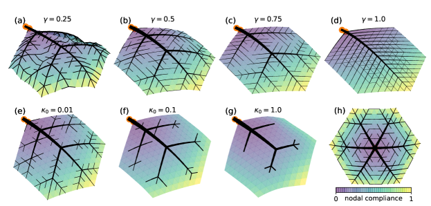
Figure 2: Compliance-optimized flat DBNs resemble real leaf venation. We optimized triangular DBNs with $N=217$ nodes and $E_{\text{triang}}=600$ edges. (a–c) For $0<\gamma<1$, optimal networks are sparse and show hierarchical organization and anastomosing reticulation. (d) At the transition $\gamma=1$ the network becomes highly reticulate and less hierarchically organized. The networks (a–d) were subject to a uniform downward load, the petiole was modeled as one additional node the position of which was fixed, and overall twists of the petiole were removed. The lamina stiffness was $\kappa_{0}=10^{-6}$. (e–g) Optimal networks reduce to just the main veins as the lamina stiffness $\kappa_{0}$ is increased. (h) An optimal network with the petiole at the center and subject to a uniform upward load. The cost parameter in (e–h) was $\gamma=1/2$, and the lamina stiffness in (h) was $\kappa_{0}=10^{-6}$. Fixed nodes are shown as red dots, each triangle is colored by the average nodal compliance $\mathbf{f}_{i}^{\top}\mathbf{u}_{i}$ of the adjacent nodes normalized by the maximum, and the line thicknesses are proportional to $\kappa_{b}^{\gamma/2}$.

Equation (2) then suggests that the elastic energy of an arbitrary number of beams elastically connected at a node $i$ [Fig. 1 (e)] can be written as,

$$V_{i}=\frac{1}{2}\sum_{b\in B_{i}}\kappa_{b}\|(R_{i}\,\mathbf{e}_{b})\times\mathbf{b}\|^{2},$$ (3)

where the sum runs over the set $B_{i}$ of edges joining at node $i$, $\kappa_{b}$ is the bending constant of edge $b$, and $\mathbf{b}$ is the unit vector pointing from node $i$ to node $j$ along the edge $b=(ij)$. The node’s equilibrium configuration is given by the local reference frame $\{\mathbf{e}_{b}\}_{b\in B_{i}}$ and $R_{i}$ compensates overall rigid rotations. We now linearize Eq. (3) by expanding both $R_{i}$ and $\mathbf{b}$ and minimizing over $R_{i}$ Note (1). We find for a network consisting of $N$ nodes,

$$V =\frac{1}{2}\mathbf{u}^{\top}\left(H_{\text{eq}}-H_{\text{or}}\right)\mathbf{u}=\frac{1}{2}\mathbf{u}^{\top}H\mathbf{u},$$ (4)

where $\mathbf{u}$ is the $3N$-dimensional vector of nodal displacements from equilibrium. The term $(1/2)\,\mathbf{u}^{\top}H_{\text{eq}}\mathbf{u}$ is the elastic energy with respect to the fixed equilibrium frame $\{\mathbf{e}_{b}\}$, while $(1/2)\,\mathbf{u}^{\top}H_{\text{or}}\mathbf{u}$ corrects for overall rotations Note (1). Given any static loads $\mathbf{f}$ on the network, the displacements satisfy $H\mathbf{u}=\mathbf{f}$. At each node, this force balance can be expressed as $\mathbf{f}_{i}=\sum_{j}(\mathbf{F}_{ij}-\mathbf{F}_{ji})$, where $\mathbf{F}_{ij}$ is the force on node $i$ due to the connection to node $j$, and $\mathbf{f}_{i}$ is the load on node $i$ Note (1).

While our model applies to generic elastic networks, we now specialize to leaf-like structures. We consider planar DBNs described by Eq. (4) and embedded in an inextensible lamina. Inextensibility of both beam network and lamina is implemented to linear order by allowing only nodal displacements $\mathbf{u}$ that satisfy $\mathbf{e}_{b}^{\top}(\mathbf{u}_{j}-\mathbf{u}_{i})=0$ for all edges $b$ Seung and Nelson (1988); Witten (2007); Note (1).

Leaves must remain flat and rigid to present a maximal area to sunlight for photosynthesis. Thus, we expect the reinforced scaffolding network to be optimized under the influence of gravitational or wind load. Maximum rigidity of a mechanical system under loads $\mathbf{f}$ leading to displacements $\mathbf{u}$ corresponds to minimum compliance $c=\mathbf{f}^{\top}\mathbf{u}=\sum_{i}\mathbf{f}_{i}^{\top}\mathbf{u}_{i}$ Bendsøe and Sigmund (2003), where $\mathbf{f}_{i}$ is the load on node $i$ and $\mathbf{u}_{i}$ is its displacement. In the following, we minimize the compliance over the set of bending constants $\kappa_{b}$ of the network. Biological networks are constrained by the amount of resources available, and by the requirement to distribute them efficiently. Following Refs. Bohn and Magnasco (2007); Durand (2007); Katifori et al. (2010a); Corson (2010); Hu and Cai (2013); Ronellenfitsch and Katifori (2016), we incorporate this by introducing the constraint $\sum_{b}\kappa_{b}^{\gamma}=K$, where the parameter $\gamma$ models the material cost of each beam and $K$ is the overall cost. A natural material constraint is the total mass of the network, which for beams following Eq. (1) corresponds to $\gamma=1/2$. More generally, $0<\gamma<1$ leads to an economy of scale promoting sparse networks Chartrand (2007). We now focus on this biologically relevant regime.

The optimal $\kappa_{b}$ are encoded in a scaling relation with the nodal forces Note (1),

$$\kappa_{b}\sim\left(\ell_{b}^{2}\,(\|\mathbf{F}_{ij}\|^{2}+\|\mathbf{F}_{ji}\|^{2})\right)^{\frac{1}{1+\gamma}},$$ (5)

where the edge $b$ connects nodes $i$ and $j$. To avoid local minima due to the non-convex constraint, we employ a numerical optimization algorithm based on simulated annealing Note (1). In the following, we start from a triangular grid in the $x$–$y$ plane representing the leaf lamina, which is attached to a petiole with fixed position and orientation {Fig. S9, Ref. Note (1)}. The entire leaf is subject to uniform load in the negative $z$ direction [Fig. 1 (d,e)], such that the compliance is now proportional to the average displacement. This is a reasonable approximation given typical leaf mass composition John et al. (2017). Including vein self-loads in this regime does not lead to markedly different optimal networks Note (1). Because the leaf lamina itself is rigid, we set the bending constants to $\kappa_{0}+\kappa_{b}$, where $\kappa_{0}$ is the lamina stiffness and the $\kappa_{b}$ are the bending constants of the network that we minimize over. The inextensibility constraint is enforced on all edges of the triangular grid irrespective of their bending rigidity, such that the lamina is always inextensible to linear order. The cost $K$ is fixed to the number of edges in the triangular grid, setting the scale for the $\kappa_{b}$. We first specialize to the regime $\kappa_{0}=10^{-6}\ll\kappa_{b}$ where the elastic properties are dominated by the venation network. Here, optimized DBNs are rigid and flat, decreasing the compliance by a factor of $\sim 100$ compared to uniform networks [Fig. 3 (c)]. Their structure exhibits the basic features of dicotyledonous leaf venation [Fig. S9 (a–e)], including a hierarchical midrib and branching and anastomosing higher order veins. This is also reflected in quantitative topological measures when comparing to real leaf networks Note (1). Mechanically optimized DBNs are structurally similar to distribution networks optimizing robust fluid transport Katifori et al. (2010a); Corson (2010); Ronellenfitsch and Katifori (2016); Hu and Cai (2013); Ronellenfitsch and Katifori (2019). This is due to a connection between hydraulic and elastic leaf network models, both of which can be seen as conservation laws (of fluid or force) with a single source and many sinks. Under the inextensibility constraint, $(1/2)\mathbf{u}^{\top}H_{\mathrm{eq}}\mathbf{u}=\sum_{i,j}(\kappa_{b}/\ell_{b}^{2})\,(u_{z,j}-u_{z,i})^{2}$, where $u_{z,i}$ are the $z$ components of the displacements Note (1). Formally identifying $\kappa_{b}/\ell_{b}^{2}$ with the hydraulic conductivity and the perpendicular displacements $u_{z,i}$ with the potential, this part of the compliance has the same form as the power dissipation minimized for flow networks and encodes only the weighted network topology. Optimal flow networks are known to correspond to topological trees Banavar et al. (2000), even though the global optimum may not be hierarchical Yan et al. (2018). Thus, the geometric term $\mathbf{u}^{\top}H_{\mathrm{or}}\mathbf{u}$ is responsible for departure from the tree-optima and induces redundant connections in mechanical networks Note (1). This intrinsic elastic mechanism stands in contrast to flow networks where only explicitly modeling additional effects such as resistance to fluctuations or damage can induce loops Katifori et al. (2010b); Hu and Cai (2013); Corson (2010).

When $\gamma>1$, the optimization problem becomes convex, and a single global minimum exists, containing a midrib but otherwise appearing featureless [Fig. S9 (d)]. The generic properties of optimal DBNs remain valid for other boundary conditions as well [Fig. S9 (h)].

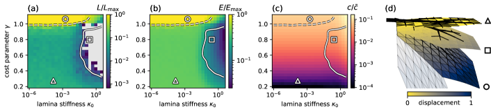
Figure 3: Topological transition and phase space of optimal DBNs with leaf boundary conditions. Each pixel in the $25\times 25$ images (a–c) corresponds to a mean over 10 annealed triangular networks with $N=92$ nodes and $E_{\text{max}}=241$ edges. (a) Network topology is encoded in the loop density $L/L_{\text{max}}$, where $L$ is the number of loops and $L_{\text{max}}=150$ is the maximum number of loops in the triangular grid. Grey pixels correspond to $L=0$. The dashed and solid lines approximately mark the transitions to maximally loopy and tree topologies, respectively. (b) Network structure as measured by the number of nonzero bending constant edges $E$ normalized by the maximum number $E_{\text{max}}$ of edges in the triangular grid. (c) The compliance $c$ of the optimized networks, normalized by the compliance $\bar{c}$ of a uniform network with identical cost $K$. The results in (a–c) remain qualitatively valid for larger networks as well Note (1). (d) Optimal networks $\bigtriangleup$, $\square$, $\Circle$, and a uniform network shown with their relative displacements under the same load. The optimal networks are also marked in panels (a–c). Displacements are measured relative to the tip of network $\Circle$.

We now proceed to study the topological transition from non-reticulate to reticulate optimal networks. The topology of planar networks is quantified by the number of loops $L=E-N+1$, as obtained from Euler’s formula. Optimal DBNs exhibit three basic topological phases [Fig. 3 (a)]. In the convex regime where $\gamma>1$ and the lamina stiffness $\kappa_{0}\lesssim 10^{-2}$, the optimal networks corresponding to the single global minimum are maximally loopy. As $\gamma$ is decreased below $1$, most loops are lost and the optimal networks feature a small number of loops that is approximately constant over a wide range of parameter values. Increasing the lamina stiffness beyond $\kappa_{0}\approx 10^{-2}$ leads to a gradual crossover into a loop-less regime, where only main and secondary veins are reinforced [Fig. S9 (e–g)]. These transitions are mirrored in the number of nonzero bending constant edges $E$ in the network, with the difference that $E$ gradually decreases as $\kappa_{0}$ is increased instead of dropping to zero [Fig. 3 (b)]. Surprisingly, the optimal compliance does not vary strongly with the optimal network topology [Fig. 3 (c, d)]. Instead, the optimal compliance is largely independent of the lamina stiffness $\kappa_{0}$ and varies strongly only with the cost parameter $\gamma$. Since $\gamma$ is expected to be fixed by geometry, this suggests that generically, it pays to invest in an optimized mechanical network, even if this means only reinforcing the main vein. Even then, the improvement in compliance is significant [Fig. 3 (c)].

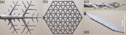
Figure 4: Biologically inspired metamaterials for flatness and rigidity. (a) Additively manufactured metamaterial based on an optimized DBN topology with $\gamma=1/2$. The vertical size is $11\,\mathrm{cm}$, the material is thermoplastic polyurethane Note (1). (b) Metamaterial based on a uniform DBN topology with equal size and total volume. Beam radii in (a, b) are proportional to $\kappa_{b}^{1/4}$, and $\kappa_{0}=0$. (c, d) Side view of the same networks clamped at the petiole. The optimized network (c) remained flat. The uniform network (d) showed a tip displacement of approximately $5\,\mathrm{cm}$.

The natural design principles of leaf venation can be applied to the design of efficient rigid metamaterials. We additively manufactured networks of connected cylindrical beams based on optimized and uniform DBN topologies with equal material volume {Fig. 4 (a, b), Ref. Note (1)}. The improvement in rigidity in the optimized manufactured network is significant, with no bending or tip displacement discernible [Fig. 4 (c)]. This is compared to the uniform network, which bends visibly [Fig. 4 (d)]. This suggests that biologically inspired elastic networks may provide design principles for discrete metamaterials.

In summary, we considered a model of discrete beam networks that is able to naturally represent non-uniform reinforcing scaffoldings of elastic sheets and networks, and applied it to leaf venation. We showed that optimal DBNs minimizing mechanical compliance under a cost constraint resemble real leaves, including a hierarchical backbone, anastomoses, and loops between the veins. Using the principles learned from nature, we designed and manufactured elastic metamaterials.

Our results may have implications for the biology of leaves and other natural materials with a combined mechanical and hydraulic function such as dragonfly wings Sun and Bhushan (2012). The relevance of fluid flow optimization for leaf venation is well-known when rationalizing loops as an evolutionary adaptation to damage or fluctuations Katifori (2018); Ronellenfitsch and Katifori (2019). At the same time, the reduction in compliance of optimized over uniform DBNs is highly significant. Thus, maximizing stiffness could result in an evolutionary advantage. Leaves are therefore in the extraordinary position to optimize two highly disparate requirements, mechanical rigidity and robust fluid transport, using the same hierarchically organized, reticulate venation network architecture. Our results may also offer a connection between the differing approaches modeling leaf vascular development as adaptive mechanisms relying on either flow Runions et al. (2014); Dimitrov and Zucker (2006); Ronellenfitsch and Katifori (2016) or mechanical Corson et al. (2010, 2009); Laguna et al. (2008); Bar-Sinai et al. (2016); Couder et al. (2002) cues. More generally, our work paves the way for detailed study of optimized mechanical networks in other biological systems such as actin-myosin networks Mizuno et al. (2007), active mechanics Ronceray et al. (2016); Noll et al. (2017), allosteric materials Rocks et al. (2017), or network control Kim et al. (2019).

Supplemental Material

I Small-angle approximation

Figure S1: Approximating a weakly bent beam of length $\ell$ (dashed line) by discrete elements (nodes are black circles). The bending angle between the discrete elements is $\alpha$, each element has length $\ell/2$, the beam’s radius of curvature is $\mathcal{R}$.

We now justify the small-angle approximation for the radius of curvature of a weakly bent beam using the setup shown in Fig. S1. The law of cosines in the shown triangle leads to

$$\cos\frac{\alpha}{2}=\frac{1}{4}\frac{\ell}{\mathcal{R}}.$$

Using the fact that $\alpha=\pi-\varepsilon$ for a small angle $\varepsilon$, we simplify the left hand side as

$$\cos\frac{\alpha}{2}=\sin\frac{\varepsilon}{2}\approx\frac{1}{2}\sin\varepsilon=\frac{1}{2}\sin\alpha,$$

where we used that $\sin\varepsilon=2\sin(\varepsilon/2)\cos(\varepsilon/2)$ and $\cos(\varepsilon/2)\approx 1$. We then find

$$\frac{1}{\mathcal{R}^{2}}=\frac{4}{\ell^{2}}\sin^{2}\alpha,$$

from which Eq. (1) follows.

II Minimization over the rotational degrees of freedom

We first show that Eq. (2) reduces to the correct elastic energy upon minimizing over the orientation of the local reference frame. We write the unit vectors defining the edges in polar coordinates as $\mathbf{b}_{1}=(\sin\theta_{1},\cos\theta_{1},0)$, $\mathbf{b}_{2}=(\sin\theta_{2},\cos\theta_{2},0)$. The reference frame is chosen as $\mathbf{e}_{1}=(1,0,0)$ and $\mathbf{e}_{2}=(-1,0,0)$. Then, the rotated reference frame can be expressed as $R\,\mathbf{e}_{1}=(\sin\phi,\cos\phi,0)$, and $R\,\mathbf{e}_{2}=-R\,\mathbf{e}_{1}$, where $\phi$ is the angle of rotation in the $x$–$y$ plane. With this, the elastic energy Eq. (2) becomes,

$$V=\frac{1}{2}\tilde{\kappa}_{b}\sin^{2}(\phi-\theta_{1})+\frac{1}{2}\tilde{\kappa}_{b}\sin^{2}(\pi+\phi-\theta_{2}).$$

In the limit of small angles, the minimizer of $V$ with respect to $\phi$ is $\phi^{*}\approx(\theta_{1}+\theta_{2}-\pi)/2$. Plugging this back in we obtain

$$V\approx\frac{1}{4}\tilde{\kappa}_{b}\,\sin^{2}(\pi+\theta_{1}-\theta_{2})=\frac{1}{4}\tilde{\kappa}_{b}\sin^{2}\alpha,$$

which agrees with Eq. (1) upon identifying $\tilde{\kappa}_{b}=2\kappa_{b}$.

III DBN bending energy

We now derive the DBN bending energy Eq. (4) from Eq. (3). We minimize the elastic energy Eq. (3) over the linearized rotation matrix which is parametrized by a vector $\mathbf{n}_{i}$ and acts as $R_{i}\,\mathbf{a}\approx\mathbf{a}+\mathbf{n}_{i}\times\mathbf{a}$ on a vector $\mathbf{a}$. We write the position of each node as $\mathbf{x}_{i}=\mathbf{x}_{i}^{(0)}+\mathbf{u}_{i}$, where $\mathbf{x}_{i}^{(0)}$ is the equilibrium position and $\mathbf{u}_{i}$ is a small displacement. To linear order, the unit vector along an edge $b=(ij)$ can be expanded as $\mathbf{b}\approx\mathbf{e}_{b}+J_{b}(\mathbf{u}_{j}-\mathbf{u}_{i})$, where the Jacobian encodes the double cross product $J_{b}\mathbf{a}=-\frac{1}{\ell_{b}}\mathbf{e}_{b}\times(\mathbf{e}_{b}\times\mathbf{a})$ with the equilibrium length $\ell_{b}$ and the equilibrium unit vector $\mathbf{e}_{b}=(\mathbf{x}_{j}^{(0)}-\mathbf{x}_{i}^{(0)})/\|\mathbf{x}_{j}^{(0)}-\mathbf{x}_{i}^{(0)}\|$. With this, we can expand

$$\|(R_{i}\,\mathbf{e}_{b})\times\mathbf{b}\|^{2} \approx\|(\mathbf{e}_{b}+J_{b}(\mathbf{u}_{j}-\mathbf{u}_{i}))\times(\mathbf{e}_{b}+\mathbf{n}_{i}\times\mathbf{e}_{b})\|^{2}$$

$$=\|D_{b}\mathbf{u}-C_{b}\mathbf{n}_{i}\|^{2},$$

where we neglected non-linear terms in $\mathbf{u}$ and $\mathbf{n}_{i}$. Here, the matrix $D_{b}$ acts as $D_{b}\mathbf{u}=\frac{1}{\ell_{b}}\mathbf{e}_{b}\times(\mathbf{u}_{j}-\mathbf{u}_{i})$, $C_{b}=\mathbb{1}-\mathbf{e}_{b}\mathbf{e}_{b}^{\top}$, and the $3N$-dimensional vector $\mathbf{u}$ contains the displacements of the $N$ nodes. At each node $i$, the linearized elastic energy is then

$$V_{i} =\frac{1}{2}\sum_{b\in B_{i}}\kappa_{b}\|D_{b}\mathbf{u}-C_{b}\mathbf{n}_{i}\|^{2}.$$ (S1)

Taking the gradient of $V_{i}$ with respect to $\mathbf{n}_{i}$ and setting it to zero using $C_{b}^{\top}C_{b}=C_{b}$ and $C_{b}^{\top}D_{b}=D_{b}$ we obtain $C_{i}\mathbf{n}_{i}=D_{i}\mathbf{u}$, where $C_{i}=\sum_{b\in B_{i}}\kappa_{b}C_{b}$ and $D_{i}=\sum_{b\in B_{i}}\kappa_{b}D_{b}$. Formally solving this linear equation for $\mathbf{n}_{i}$, plugging the result into Eq. (S1), and summing over all nodes $i$, we arrive at Eq. (4) with

$$H_{\text{eq}}=\sum_{i}\sum_{b\in B_{i}}\kappa_{b}D_{b}^{\top}D_{b}$$ (S2)

and

$$H_{\text{or}}=\sum_{i}D_{i}^{\top}C_{i}^{-1}D_{i}.$$ (S3)

We note that although we derived Eq. (4) from Eq. (2), which models only the lowest bending mode, larger DBNs can naturally model higher modes as well if they contain many connected nodes arranged in a line, providing a fine discretization of a continuum beam.

III.1 Planar networks

For planar, inextensible networks, it can be shown that only the $z$ component of the displacements $\mathbf{u}$ is nonzero (Section VIII). With this, Eq. (S2) corresponds to the weighted network Laplacian,

$$\frac{1}{2}\mathbf{u}^{\top}H_{\mathrm{eq}}\mathbf{u} =\frac{1}{2}\sum_{i}\sum_{b\in B_{i}}\frac{\kappa_{b}}{\ell_{b}^{2}}\|\mathbf{e}_{b}\times(\mathbf{u}_{j}-\mathbf{u}_{i})\|^{2}$$

$$=\sum_{i,j}\frac{\kappa_{b}}{\ell_{b}^{2}}(u_{z,j}-u_{z,i})^{2}.$$

This expression depends only on the weighted topology of the elastic network and not on the geometry at all. In contrast, Eq. (S3) can not be written in a purely topological way and encodes the geometry and weights in a nontrivial way. We find in terms of the displacements,

$$\frac{1}{2}\mathbf{u}^{\top}H_{\mathrm{or}}\mathbf{u} =\frac{1}{2}\sum_{i}\left(\sum_{b\in B_{i}}\frac{\kappa_{b}}{\ell_{b}}\mathbf{e}_{b}\times(\mathbf{u}_{j}-\mathbf{u}_{i})\right)^{\top}C_{i}^{-1}\left(\sum_{b\in B_{i}}\frac{\kappa_{b}}{\ell_{b}}\mathbf{e}_{b}\times(\mathbf{u}_{j}-\mathbf{u}_{i})\right)$$

$$=\frac{1}{2}\sum_{i}\left(\sum_{b\in B_{i}}\frac{\kappa_{b}}{\ell_{b}}(u_{z,j}-u_{z,i})\,\mathbf{e}_{b}^{\perp}\right)^{\top}C_{i}^{-1}\left(\sum_{b\in B_{i}}\frac{\kappa_{b}}{\ell_{b}}(u_{z,j}-u_{z,i})\,\mathbf{e}_{b}^{\perp}\right),$$

where $\mathbf{e}_{b}$ is rotated by $\pi/2$ in the $x$–$y$ plane into $\mathbf{e}_{b}^{\perp}$. The matrix $C_{i}^{-1}=\left(\sum_{b\in B_{i}}\kappa_{b}\,(\mathbb{1}-\mathbf{e}_{b}\mathbf{e}_{b}^{\top})\right)^{-1}$ depends on both stiffnesses and local geometry at the node $i$.

IV Nodal force balance

We now derive the nodal force balance from Eq. (S1). Rewriting in terms of three-dimensional vectors and making the edges $b=(ij)$ explicit the total network energy $V=\sum_{i}V_{i}$ reads

$$V =\frac{1}{2}\sum_{i,j}\kappa_{ij}\|C_{ij}\mathbf{n}_{i}-\ell_{ij}^{-1}\mathbf{e}_{ij}\times(\mathbf{u}_{j}-\mathbf{u}_{i})\|^{2}.$$

Using $\partial V/\partial\mathbf{n}_{i}^{\top}=0$, the net force on node $i$ is

$$\mathbf{F}_{i} =-\frac{\partial V}{\partial\mathbf{u}_{i}^{\top}}=\sum_{j}(\mathbf{F}_{ij}-\mathbf{F}_{ji}),$$

where we used that each nodal displacement $\mathbf{u}_{i}$ appears in $V_{i}$ and in all $V_{j}$ that are connected to node $i$. The forces are

$$\mathbf{F}_{ij}=-\frac{\kappa_{ij}}{\ell_{ij}}\mathbf{e}_{ij}\times\left(C_{ij}\mathbf{n}_{i}-\ell_{ij}^{-1}\mathbf{e}_{ij}\times(\mathbf{u}_{j}-\mathbf{u}_{i})\right).$$

Here, $\kappa_{ij}=\kappa_{ji}$, $\ell_{ij}=\ell_{ji}$, and $C_{ij}=C_{ji}$. Using the definition of $C_{ij}=\mathbb{1}-\mathbf{e}_{ij}\mathbf{e}_{ij}^{\top}$, the magnitudes are,

$$\|\mathbf{F}_{ij}\|^{2} =\frac{\kappa_{ij}^{2}}{\ell_{ij}^{2}}\|C_{ij}\mathbf{n}_{i}-\ell_{ij}^{-1}\mathbf{e}_{ij}\times(\mathbf{u}_{j}-\mathbf{u}_{i})\|^{2}.$$ (S4)

V Constrained Optimization

We adapt the global approach outlined in Ref. Katifori et al. (2010a). The Lagrangian corresponding to the constrained minimization problem is

$$\mathcal{L}(\{\kappa_{b}\})=c(\{\kappa_{b}+\kappa_{0}\})+\lambda\big{(}\sum_{b}\kappa_{b}^{\gamma}-K\big{)},$$

where $c=\mathbf{f}^{\top}\mathbf{u}$ is the compliance and $\lambda$ is a Lagrange multiplier. Taking the gradient with respect to $\kappa_{b}$ and combining with Eq. (S4) leads to the scaling relation Eq. (5). We numerically solve for the $\kappa_{b}$ using the iteration

$$\tilde{\kappa}_{b}^{(n+1)} =\left(-(\kappa_{b}^{(n)})^{2}\frac{\partial c(\{\kappa_{b}^{(n)}+\kappa_{0}\})}{\partial\kappa_{b}}\right)^{1/(\gamma+1)}$$

$$\kappa_{b}^{(n+1)} =\frac{\tilde{\kappa}_{b}^{(n+1)}}{\left(\sum_{b^{\prime}}(\tilde{\kappa}_{b^{\prime}}^{(n+1)})^{\gamma}\right)^{1/\gamma}},$$ (S5)

where the second step fixes the Lagrange multiplier by enforcing the constraint. Combining Eq. (S5) with a variant of simulated annealing leads to approximate global minimization. At every $N_{\mathrm{therm}}$-th step of the iteration Eq. (S5), the $\{\kappa_{b}\}$ are first thermalized by convolving with a Gaussian kernel $G_{ab}\sim\exp(-d_{ab}^{2}/(2\sigma^{2}))$ where $d_{ab}$ is the Euclidean distance between edges $a$ and $b$ and where the scale $\sigma$ is decreased after each thermalization. Then, multiplicative noise $\sim\exp(s\,\xi)$, where $\xi$ is normally distributed and $s\sim\mathcal{O}(1)$, is applied. After a set number of thermalization steps, Eq. (S5) is iterated until convergence.

VI Metamaterials

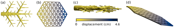
Figure S2: (a) 3D mesh used to manufacture the optimized network from Fig. 4 (a). (b) 3D mesh used to manufacture the uniform network from Fig. 4 (b). (c, d) FEM simulations of the meshes from (a,b) clamped at the left side with downward gravitational load.

3D meshes [Fig. S2 (a,b)] were constructed from cylinders with spherical end-caps, with cylinder radii taken from optimal and uniform DBN models. The metamaterials were commercially manufactured from thermoplastic polyurethane (Materialise nv, Leuven, Belgium). Finite Element Method simulations [Fig. S2 (c,d)] were performed using the MATLAB 2018b PDE Toolbox (The MathWorks, Inc., Natick, MA) and are consistent with the experimental results shown in Fig. 4. Material properties were Young’s Modulus $Y=85\,\mathrm{MPa}$, density $\rho=1100\,\mathrm{kg}\,\mathrm{m}^{-3}$, Poisson’s ratio $\nu=0.49$.

VII Continuum limit

Here we demonstrate that the bending energy Eq. (4) in the continuum limit of an initially flat, uniform sheet in equilibrium is equivalent to the Helfrich free energy Helfrich (1973); Safran (1999); Seung and Nelson (1988),

$$F=\int_{A}(\kappa_{1}H^{2}+\kappa_{2}K)\,dA,$$ (S6)

where $H$ and $K$ are the surface’s mean and Gaussian curvatures, respectively, $\kappa_{1}$,$\kappa_{2}$ are elastic constants, and the integral is over the surface of the sheet $A$. We choose a triangular grid to model the flat sheet in the $x$–$y$ plane and set all the bending constants $\kappa_{b}$ to unity. The inextensibility constraint is then equivalent to only allowing displacements in the $z$ direction, $\mathbf{u}=(0,0,\mathbf{u}_{z}^{\top})^{\top}$, since all local in-plane displacements are forbidden. At each node, the unit vectors in the directions of the edges are

$$\mathbf{e}_{1} =(1,0,0)^{\top}, \mathbf{e}_{2} =(1/2,\sqrt{3}/2,0)^{\top},$$

$$\mathbf{e}_{3} =(1/2,-\sqrt{3}/2,0)^{\top}, \mathbf{e}_{4} =-\mathbf{e}_{1},$$

$$\mathbf{e}_{5} =-\mathbf{e}_{2}, \mathbf{e}_{6} =-\mathbf{e}_{3},$$

and the matrix $C_{i}=\operatorname{diag}(3,3,6)$. In the limit where the edge lengths $\ell$ tend to zero, the sheet’s displacements are approximated by a height function $u_{z}=h(x,y)$. The expressions involving the matrices $D_{b}$ can then be written as $D_{b}\mathbf{u}\approx\ell^{-1}\mathbf{e}_{b}\times(0,0,h(x+\ell\,(\mathbf{e}_{b})_{x},y+\ell\,(\mathbf{e}_{b})_{y})-h(x,y))^{\top}$. Plugging this form into Eq. (4), expanding to lowest order in $\ell$ and summing over all vertices we find for the total bending energy,

$$V\approx\frac{3}{16}\sum_{i}\left(3(h_{xx}+h_{yy})^{2}-4(h_{xx}h_{yy}-h_{xy}^{2})\right)\ell^{2}.$$ (S7)

Using the small-gradient expansions do Carmo (1988) of the mean curvature $H\approx h_{xx}+h_{yy}$ and the Gaussian curvature $K\approx h_{xx}h_{yy}-h_{xy}^{2}$, and the area element $dA\approx\ell^{2}\sqrt{3}/2$ corresponding to hexagons around each node, in the limit $\ell\to 0$ the sum Eq. (S7) tends to the integral Eq. (S6) with the elastic constants $\kappa_{1}=3\sqrt{3}/8$ and $\kappa_{2}=-\sqrt{3}/2$.

VIII Mechanical constraints

VIII.1 Edge inextensibility

We now discuss the effect of inextensible edges to lowest order. The length of each edge $b=(ij)$ can be written as

$$\ell_{b} =\sqrt{\left(\mathbf{x}_{i}^{(0)}-\mathbf{x}_{j}^{(0)}+\mathbf{u}_{i}-\mathbf{u}_{j}\right)^{2}}$$

$$\approx\ell^{(0)}_{b}+\mathbf{e}_{b}^{\top}(\mathbf{u}_{i}-\mathbf{u}_{j}),$$

where $\mathbf{x}_{i}^{(0)}$ is the equilibrium position of node $i$, $\mathbf{e}_{b}=(\mathbf{x}^{(0)}_{i}-\mathbf{x}_{j}^{(0)})/\|\mathbf{x}^{(0)}_{i}-\mathbf{x}_{j}^{(0)}\|$ is the edge unit vector and we expanded to linear order. The inextensibility constraint is then equivalent to allowing only displacements satisfying the constraint $\mathbf{e}_{b}^{\top}(\mathbf{u}_{i}-\mathbf{u}_{j})=0$ for all edges $b$. This can be implemented by assembling all these constraints into a matrix $Q$ acting on the vector of all displacements in the network and demanding

$$0=Q\mathbf{u}=\begin{pmatrix}Q_{x}\\ Q_{y}\\ 0\end{pmatrix}\begin{pmatrix}\mathbf{u}_{x}\\ \mathbf{u}_{y}\\ \mathbf{u}_{z}\end{pmatrix}.$$ (S8)

Here, $\mathbf{u}_{x,y,z}$ are the $x$, $y$, and $z$ components of the displacements, and we used the fact that we consider planar networks such that all unit vectors $\mathbf{e}_{b}$ lie in the $x$–$y$ plane. The matrix $Q$ is also known as the compatibility matrix Lubensky et al. (2015) of the elastic network, and its nullspace $Q\mathbf{u}=0$ encodes the allowed displacements satisfying the inextensibility constraint. Inspecting Eq. (S8), we find that all displacements in the $z$ direction (perpendicular to the network) $\mathbf{u}_{z}$ are allowed.

Any remaining degrees of freedom $\mathbf{u}_{x,y}$ must then be in-plane. Non-degenerate triangulations (including triangular grids as used in the main paper) possess no such degrees of freedom except for Euclidean motions (overall rotations and translations): each triangle is rigid by itself, and adding another triangle to an already rigid finite triangular grid can not introduce in-plane soft modes as long as it is joined by one of its sides. This induction step can be seen as follows. Each new triangle contributes two new edges and one new node. Two new constraints corresponding to two new edges are introduced. Since all nodes except for the new one are already rigid, they will remain so, and their in-plane degrees of freedom are all $\mathbf{u}_{x,y;i}=0$. The new in-plane degree of freedom $\mathbf{u}_{x,y}^{*}$ must then satisfy $\mathbf{e}_{1}^{*}{}^{\top}\mathbf{u}_{x,y}^{*}=0$ and $\mathbf{e}_{2}^{*}{}^{\top}\mathbf{u}_{x,y}^{*}=0$, where $\mathbf{e}_{1,2}^{*}$ are the unit vectors corresponding to the newly added edges. We assumed the triangulation to be non-degenerate, meaning that the new edges are not parallel. From this, $\mathbf{u}^{*}_{x,y}=0$ immediately follows.

We conclude that to linear order, the allowed displacements for non-degenerate triangulations are the $\mathbf{u}_{z}$ in the $z$ direction, perpendicular to the planar network, as well as Euclidean transformations (overall rotations and translations).

VIII.2 Lamina inextensibility

In many biological networks such as leaves, not just the veins are inextensible, but also the lamina itself. Stretching of a triangulated sheet can be modeled using springs between nearest neighbors Seung and Nelson (1988); Witten (2007). Because the edges in the DBNs considered here are inextensible, this automatically models an inextensible lamina as well.

VIII.3 Numerical implementation

For the numerical optimizations, we explicitly construct a constraint matrix by taking the compatibility matrix $Q$ and adding rows corresponding to (i) the removal of overall an twist degree of freedom along the $x$ axis and (ii) clamping of the petiole. We then numerically compute a matrix $\Phi$ of basis vectors of its nullspace and proceed to use the projected Hessian $H^{\prime}=\Phi H\Phi^{\top}$, which encodes only the allowed degrees of freedom. We constrain the lengths of the triangular grid topology without removing edges whose stiffness is set to zero by the optimization algorithm, such that the lamina always remains inextensible.

VIII.4 Soft modes

Even with the constraints as implemented above, in-plane soft modes are possible, for instance if the underlying network is chosen to be non-triangular, with hypostatic coordination number $z<4$. However, this is unphysical in the biological systems we aim to model. Out-of-plane soft modes are possible if the lamina stiffness $\kappa_{0}=0$ and a node is not connected by any nonzero $\kappa_{b}$ to other nodes. Then the constraints allow arbitrary displacements in $z$ direction that are no longer energetically penalized. This case is not observed in optimized networks, as it would lead to very large compliance (the load would be parallel to the soft mode displacement).

IX Optimization with self-loads

While for many biological systems such as leaves uniform loads $\mathbf{g}$ are a reasonable approximation John et al. (2017), the case of self-loads (i.e., loads that depend on the edge stiffnesses) can be considered as well. In general, the mathematical structure of self-loaded optimization problems changes significantly Bruyneel and Duysinx (2005), making the numerical methods employed in the main paper inappropriate. Here, we consider a simple model of self-loads and derive an iterative scheme to solve the associated KKT (Karush–Kuhn–Tucker) optimality equations.

IX.1 Numerical optimization with self-loads

To include self-loads we write the compliance in the form

$$c=\mathbf{f}^{\top}H\mathbf{f},$$

where now both the Hessian $H=H(\{\kappa_{e}\})$ and the loads $\mathbf{f}=\mathbf{f}(\{\kappa_{e}\})$ are functions of the stiffnesses. The gradient of the compliance with respect to the stiffnesses $\kappa_{e}$ is then

$$\frac{\partial c}{\partial\kappa_{e}}=-\mathbf{f}^{\top}\frac{\partial H}{\partial\kappa_{e}}\mathbf{f}+2\,\mathbf{f}^{\top}H\frac{\partial\mathbf{f}}{\partial\kappa_{e}}.$$ (S9)

Using the method of Lagrange multipliers to include the cost constraint and the inequality constraint $\kappa_{e}\geq 0$, we derive the KKT equations

$$\kappa_{e}\frac{\partial c}{\partial\kappa_{e}}+\lambda\gamma\,\kappa_{e}^{\gamma} =0$$ (S10)

$$\sum_{e}\kappa_{e}^{\gamma}=K.$$

We first solve for the Lagrange multiplier by summing over Eq. (S10), obtaining

$$\lambda=\frac{1}{\gamma K}\sum_{e}\left(\kappa_{e}\mathbf{f}^{\top}\frac{\partial H}{\partial\kappa_{e}}\mathbf{f}-2\kappa_{e}\,\mathbf{f}^{\top}H\frac{\partial\mathbf{f}}{\partial\kappa_{e}}\right).$$

Next, we multiply Eq. (S10) by $\kappa_{e}$ and rearrange to

$$\kappa_{e}^{\gamma+1}\left(\lambda\gamma+2\kappa_{e}^{1-\gamma}\mathbf{f}^{\top}H\frac{\partial\mathbf{f}}{\partial\kappa_{e}}\right)=\kappa_{e}^{2}\,\mathbf{f}^{\top}\frac{\partial H}{\partial\kappa_{e}}\mathbf{f}.$$

Since the right-hand side of this equation is non-negative, the left-hand side is also. Furthermore, the right-hand side corresponds to the same expression involving physical forces as in the main paper. We can rearrange the expression above into the self-consistency equation

$$\kappa_{e}=\left(\frac{\kappa_{e}^{2}\,\mathbf{f}^{\top}\frac{\partial H}{\partial\kappa_{e}}\mathbf{f}}{\lambda\gamma+2\kappa_{e}^{1-\gamma}\mathbf{f}^{\top}H\frac{\partial\mathbf{f}}{\partial\kappa_{e}}}\right)^{\frac{1}{1+\gamma}}.$$

From this we construct the iterative scheme

$$\tilde{\kappa}_{e}^{(n+1)} =\left.\left|\frac{\kappa_{e}^{2}\,\mathbf{f}^{\top}\frac{\partial H}{\partial\kappa_{e}}\mathbf{f}}{\lambda\gamma+2\kappa_{e}^{1-\gamma}\mathbf{f}^{\top}H\frac{\partial\mathbf{f}}{\partial\kappa_{e}}}\right|^{\frac{1}{1+\gamma}}\right.^{(n)}$$

$$\kappa_{e}^{(n+1)} =K^{1/\gamma}\frac{\tilde{\kappa}_{e}^{(n)}}{\left(\sum_{f}(\tilde{\kappa}_{f}^{(n)})^{\gamma}\right)^{1/\gamma}},$$

where the absolute value is taken to avoid negative values that may appear due to numerical issues at small values of $\kappa_{e}$. The constraint is explicitly enforced at each step to prevent numerical constraint drifting.

IX.2 A simple model for mass self-loads

We now construct a simple model for self-loads based on vein mass. We assume that the mass of each vein can be modeled as

$$m_{e}=a\,\kappa_{e}^{\alpha},$$

where $a$ is a constant of proportionality and $\alpha$ is a parameter. We expect the biologically relevant regime to be close to $\alpha=1/2$ (solid cylindrical beams). In this case, $a=\rho\ell^{3/2}\sqrt{\pi/Y}$. With this, we write the nondimensional perpendicular load at each node $i$ as

$$f_{z,i}=(1-\beta)\,\bar{f}+\frac{\beta}{N}\,\frac{1}{N_{n}}\sum_{(e,i)}\kappa_{e}^{\alpha},$$

where $\bar{f}$ is the dimensionless load due to the lamina, $\beta$ controls the overall proportion of vein load and lamina load, and the sum is over all $N_{n}$ edges $e$ neighboring node $i$. The additional factor of $1/N$, where $N$ is the number of nodes in the network, serves to bring the two terms to roughly the same scale. Any overall constants of proportionality are absorbed into the total cost $K$.

IX.3 Results

Since the biological regime is expected to be near $\alpha=1/2$, the following, we specialize the case $\alpha=1/2$ and $\gamma=1/2$. We also set $\bar{f}=1/N$, where $N$ is the number of nodes in the network and look at the biologically relevant regime where $0\leq\beta\leq 0.5$. We note that the fraction of vein mass to total mass $\mu$ can only be evaluated a posteriori, but is generally observed to be close to $\beta$ with the normalizations chosen above.

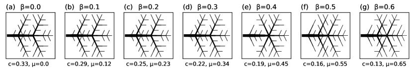
Figure S3: Optimal network topologies including self-loads with parameter $\beta$ describing the ratio between uniform lamina load and vein load and optimal compliance $c$. The final proportion $\mu$ of vein weight to total weight is calculated a posteriori. For values of $\mu\lesssim 0.34$, the optimal network topology is identical. Thus, no self-loads ($\beta=0$) are a reasonable approximation of real biological networks.

We find that up to a value of $\mu\approx 0.35$, the optimal networks with self-loads have the same topology (but not compliance value or exact numerical value of the $\kappa_{e}$) as those with $\beta=0$ (no self loads), such that neglecting self-loads appears to be a reasonable approximation (Fig. S3). Numerical experiments also indicate that in this regime, the two algorithms with and without self-loads converge to the same final network topology from identical initial conditions if no simulated annealing is used. For larger values of $0.4\leq\beta\leq 0.6$ the optimal topologies start to differ, but not in a drastic way. In the less biologically relevant regime $\beta\gg 0.6$, the numerical scheme suffers from instabilities and often does not converge.

X Scaling of the phase space of optimal DBNs

Here we present a size scaling analysis of the topological phase space shown in Fig. 3 of the main paper. While the phase space there was computed for networks with 92 nodes, here we show slices through the phase space for larger networks. We consider slices at $\gamma=0.5$ and $\kappa_{0}=10^{-3}$ and parametrize the networks by the linear number of nodes $M$ along the midrib. For the triangular networks we consider, the total number of nodes $N\sim\mathcal{O}(M^{2})$. The scaling of the number of loops is shown in Fig. S4, the scaling of the number of nonzero edges is shown in Fig. S5, and the scaling of the compliance is shown in Fig. S6. We estimate the number of nonzero edges by thresholding the results of the optimization at $\kappa_{b}=10^{-8}$ and considering all edges with smaller bending stiffness as absent. Similarly, we estimate the number of nodes by computing the weighted degree $d_{i}=(1/n)\sum_{j}\kappa_{ij}$ of each node $i$ in the original triangular network with $n$ neighbors, and again count nodes with $d_{i}<10^{-8}$ as absent. Each data point in the aforementioned figures shows an average over at least 10 optimizations. All curves for different network sizes collapse after rescaling, suggesting that the phase space shown in Fig. 3 of the main paper is robust as network size is varied.

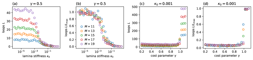
Figure S4: Scaling of the number of loops. (a) Number of loops at slice through the phase space at $\gamma=0.5$. (b) Number of loops normalized by the maximum at slice through the phase space at $\gamma=0.5$. (c) Number of loops at slice through the phase space at $\kappa_{0}=0.001$. (d) Number of loops normalized by the maximum at slice through the phase space at $\kappa_{0}=0.001$.

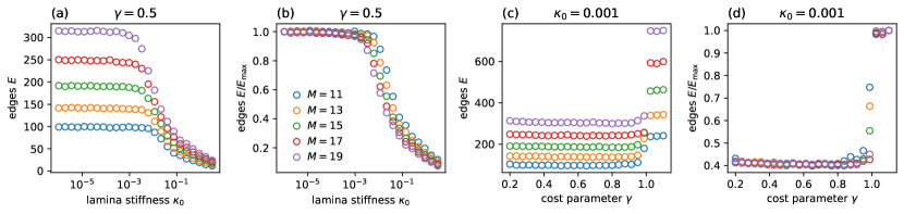
Figure S5: Scaling of the number of nonzero edges. (a) Number of edges at slice through the phase space at $\gamma=0.5$. (b) Number of edges normalized by the maximum at slice through the phase space at $\gamma=0.5$. (c) Number of edges at slice through the phase space at $\kappa_{0}=0.001$. (d) Number of edges normalized by the maximum at slice through the phase space at $\kappa_{0}=0.001$.

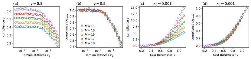
Figure S6: Scaling of the compliance. (a) Compliance at slice through the phase space at $\gamma=0.5$. (b) Compliance normalized by the compliance of a uniform network with identical cost at slice through the phase space at $\gamma=0.5$. (c) Compliance at slice through the phase space at $\kappa_{0}=0.001$. (d) Compliance normalized by the compliance of a uniform network with identical cost at slice through the phase space at $\kappa_{0}=0.001$.

XI Three-dimensional optimal DBNs

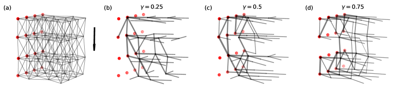
Figure S7: Three-dimensional optimal DBNs fixed at one side. (a) Tetrahedral base network with fixed nodes indicated in red. The uniform load $\mathbf{f}$ is shown as a black arrow. (b–d) Optimal networks obtained using simulated annealing with cost parameters $\gamma=0.25,0.5,0.75$ and $\kappa_{0}=10^{-4}$. Line widths are proportional to $\kappa_{b}^{\gamma/2}$.

Here we show that the DBN model introduced in the main paper can be used to model fully three-dimensional networks of connected bending beams as well. As the base topology, we take a three-dimensional tetrahedral network [Fig. S7 (a)]. Since such a network is perfectly rigid under the inextensibility constraint, for the purposes of this proof of concept, we remove the constraint. We note that for realistic applications, it would be necessary to introduce a stretching energy including a relationship between stretching and bending stiffnesses of each beam. Optimal networks fixed at one side and under uniform perpendicular load show similar features as sheet-like DBNs [Fig. S7 (b–d)].

XII Topological comparison to real leaf networks

In this section, we compare the topology of optimized DBNs to that of real leaf networks. In Ref. Blonder et al. (2020), Blonder et al. introduced the Minimum Spanning Tree (MST) ratio as an easily computable topological metric to characterize leaf networks over many scales. For a generic weighted network embedded in space, the MST ratio is defined as

$$\text{MST ratio}=\frac{\text{length of all edges in a minimum spanning tree}}{\text{total length of all edges}}.$$ (S11)

To calculate the MST, we choose the inverse edge diameter as the weight to preferentially incorporate large veins and then employ Kruskal’s algorithm.

Since leaf networks exhibit different structure at different scales, the MST ratio is calculated not just for the entire network, but also for pruned networks where all edges below a certain radius $r_{\mathrm{min}}$ are discarded. The resulting values are plotted as a function of $r_{\mathrm{min}}$ to obtain a graph characterizing the topology of the network. We calculated this measure for three leaf networks from the data set of Ref. Ronellenfitsch et al. (2015) and found similar characteristic curves as Blonder et al. [Fig. S8 (a) and Fig. S9].

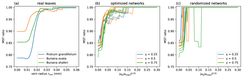
Figure S8: Topology of real leaf networks and optimized DBNs using the multi-scale MST ratio. (a) MST ratios for the three real leaf networks shown in Fig. S9. MST ratios are calculated for the network where all veins with radius less than $r_{\mathrm{min}}$ are discarded. (b) MST ratios for optimized annealed DBNs with $N=722$ nodes and $E=861$ edges and values of $\gamma\in\{0.25,0.5,0.75\}$. The value $(\kappa_{e}/\kappa_{\mathrm{max}})^{1/4}$ was used as a proxy for vein radius, corresponding to solid cylindrical beams. Here, $\kappa_{\mathrm{max}}$ is the maximum value of $\kappa_{e}$ over the entire network. (c) MST ratio curves for the same networks as in panel (b), but with the $\kappa_{e}$ randomly shuffled.

Generally, for small $r_{\mathrm{min}}$ the MST ratio is approximately constant, indicating that small veins are approximately equally distributed between loops and branches. After some critical radius, the MST ratio steeply increases as more loops than branches are removed. As the larger scales of the network are reached, the MST ratio is characterized by jumps whenever a large loop is disconnected. Finally, as all loops are removed, the MST ratio tends to 1.

We compared these results to the MST ratios of the largest optimized DBNs that were computationally feasible ($N=722$ nodes) with reasonable values of the cost parameter $\gamma\in\{0.25,0.5,0.75\}$. Despite the fact that the largest DBNs are smaller than real leaf networks by a factor between approximately 20 and 50 and that the real leaf networks show considerably more variation, the MST ratio curves are comparable, demonstrating that optimal DBNs exhibit similar topological features as real leaf networks [Fig. S8 (b)]. The same is not true when the nonzero $\kappa_{e}$ are randomly shuffled and the MST ratios recomputed [Fig. S8 (c)], demonstrating that weighted topology and hierarchical structure of real leaf networks are quantitatively reproduced in optimized DBNs.

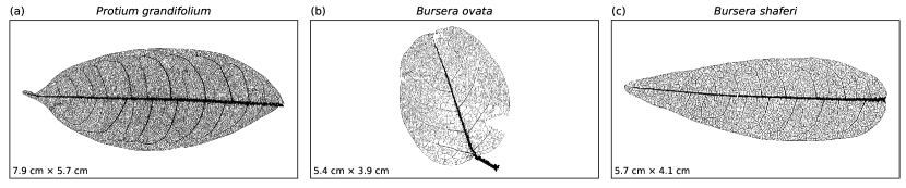
Figure S9: Discretized leaf networks used to compare to optimized DBNs. (a) Protium grandifolium. $N=45324$ nodes, $E=53772$ edges. (b) Bursera ovata. $N=24692$ nodes, $E=26692$ edges. (c) Bursera shaferi. $N=19274$ nodes, $E=21487$ edges. The dimensions of each panel are indicated in the corners.