A Restricted Dual Peaceman-Rachford Splitting Method for QAP 

Abstract

We revisit and strengthen splitting methods for solving doubly nonnegative, DNN, relaxations of the quadratic assignment problem, QAP. We use a modified restricted contractive splitting method, rPRSM, approach. Our strengthened bounds and new dual multiplier estimates improve on the bounds and convergence results in the literature.

1 Introduction

We revisit and strengthen splitting methods for solving doubly nonnegative, DNN, relaxations of the quadratic assignment problem, QAP. We use a modified restricted contractive Peaceman-Rachford splitting method, rPRSM approach. We obtain strengthened bounds from improved lower and upper bounding techniques, and from strengthened dual multiplier estimates. We compare with recent results in [24]. In addition, we provide a new derivation of facial reduction, FR, and the gangster constraints, and show the strong connections between them.

The quadratic assignment problem, QAP, is one of the fundamental combinatorial optimization problems in the fields of optimization and operations research, and includes many fundamental applications. It is arguably one of the hardest of the NP-hard problems. The QAP models real-life problems such as facility location. Suppose that we are given a set of $n$ facilities and a set of $n$ locations. For each pair of locations $(s,t)$ a distance $B_{st}$ is specified, and for each pair of facilities $(i,j)$ a weight or flow $A_{i,j}$ is specified, e.g., the amount of supplies transported between the two facilities. In addition, there is a location (building) cost $C_{is}$ for assigning a facility $i$ to a specific location $s$. The problem is to assign each facility to a distinct location with the goal of minimizing the sum over all facility-location pairs of the distances between locations multiplied by the corresponding flows between facilities, along with the sum of the location costs. Other applications include: scheduling, production, computer manufacture (VLSI design), chemistry (molecular conformation), communication, and other fields, see e.g., [13, 16, 29, 21, 20]. Moreover, many classical combinatorial optimization problems, including the traveling salesman problem, maximum clique problem, and graph partitioning problem, can all be expressed as a QAP, see e.g., [4, 26]. For more information about QAP, we refer the readers to [7, 25].

That the QAP 1.1 is NP-hard is given in [15]. The cardinality of the feasible set of permutation matrices $\Pi$ is $n!$ and it is known that problems typically have many local minima. Up to now, there are three main classes of methods for solving QAP. The first type is heuristic algorithms, such as genetic algorithms, e.g., [10], ant systems [14] and meta-heuristic algorithms, e.g., [3]. These methods usually have short running times and often give optimal or near-optimal solutions. However the solutions from heuristic algorithms are not reliable and the performance can vary depending on the type of problem. The second type is branch-and-bound algorithms. Although this approach gives exact solutions, it can be very time consuming and in addition requires strong bounding techniques. For example, obtaining an exact solution using the branch-and-bound method for $n=30$ is still considered to be computationally challenging. The third type is based on semidefinite programming, SDP. Semidefinite programming is proven to have successful implementations and provides tight relaxations, see [2, 33]. There are many well-developed SDP solvers based on e.g., interior point methods, e.g., [32, 1, 23]. However, the running time of the interior point methods do not scale well, and the SDP relaxations become very large for the QAP. In addition, adding additional polyhedral constraints such as interval constraints, can result in having $O(2n^{2})$ constraints, a prohibitive number for interior point methods.

Recently, Oliveira at el., [24] use an alternating direction method of multipliers, ADMM, to solve a facially reduced, FR, SDP relaxation. The FR allows for a natural splitting of variables between the SDP cone and polyhedral constraints. The algorithm provides competitive lower and upper bounds for QAP. In this paper, we modify and improve on this work.

1.1 Background

It is known e.g., [12], that many of the QAP models, such as the facility location problem, can be formulated using the trace formulation:

$$p^{*}_{\textbf{QAP}}:=\min_{X\in\Pi}\langle AXB-2C,X\rangle,$$ (1.1)

where $A,B\in\mathbb{S}^{n}$ are real symmetric $n\times n$ matrices, $C$ is a real $n\times n$ matrix, $\langle\cdot,\cdot\rangle$ denotes the trace inner product, i.e., $\langle Y,X\rangle=\tr(YX^{T})$, and $\Pi$ denotes the set of $n\times n$ permutation matrices.

We use the following notation from [24]. We denote the matrix lifting

$$Y:=\left(\begin{array}[]{c}1\\ x\end{array}\right)(1~{}~{}x^{T})\in\mathbb{S}^{n^{2}+1},\quad x={\rm vec}(X)\in\mathbb{R}^{n^{2}},$$ (1.2)

where $\operatorname{{vec}}(X)$ is the vectorization of the matrix $X\in\mathbb{R}^{n\times n}$, columnwise. Then $Y\in\textit{$\mathbb{S}^{n^{2}+1}_{+}$}$, the space of real symmetric positive semidefinite matrices of order $n^{2}+1$, and the rank, $\rank(Y)=1$. Indexing the rows and columns of $Y$ from $0$ to $n^{2}$, we can express $Y$ in 1.2 using a block representation as follows:

$$Y=\begin{bmatrix}Y_{00}&\bar{y}^{T}\\ \bar{y}&\overline{Y}\end{bmatrix},\quad\textit{$\bar{y}$}=\begin{bmatrix}Y_{(10)}\\ Y_{(20)}\\ \vdots\\ Y_{(n0)}\end{bmatrix},\quad\hbox{and}\quad\textit{$\overline{Y}=xx^{T}$}=\begin{bmatrix}\overline{Y}_{(11)}&\overline{Y}_{(12)}&\cdots&\overline{Y}_{(1n)}\\ \overline{Y}_{(21)}&\overline{Y}_{(22)}&\cdots&\overline{Y}_{(2n)}\\ \vdots&\ddots&\ddots&\vdots\\ \overline{Y}_{(n1)}&\ddots&\ddots&\overline{Y}_{(nn)}\end{bmatrix},$$ (1.3)

where

$$\textit{$\overline{Y}_{(ij)}=X_{:i}X_{:j}^{T}$}\in\mathbb{R}^{n\times n},\,\forall i,j=1,\ldots,n,\ Y_{(j0)}\in\mathbb{R}^{n},\forall j=1,\ldots,n,\text{ and }\ x\in\mathbb{R}^{n^{2}}.$$

Let

$$L_{Q}=\begin{bmatrix}0&-(\operatorname{{vec}}(C)^{T})\\ -\operatorname{{vec}}(C)&B\otimes A\end{bmatrix},$$

where $\otimes$ denotes the Kronecker product. With the above notation and matrix lifting, we can reformulate the QAP 1.1 equivalently as

$$\begin{array}[]{rl}p^{*}_{\textbf{QAP}}=\min&\langle AXB-2C,X\rangle=\langle L_{Q},Y\rangle\\ \text{s.t.}&Y:=\begin{pmatrix}1\\ x\end{pmatrix}\begin{pmatrix}1\cr x\end{pmatrix}^{T}\in\mathbb{S}^{n^{2}+1}_{+}\\ &X=\operatorname{{Mat}}(x)\in\Pi,\end{array}$$ (1.4)

where $\operatorname{{Mat}}=\operatorname{{vec}}^{*}$.

In [33], Zhao et al. derive an SDP relaxation as the dual of the Lagrangian relaxation of a quadratically constrained version of 1.4, i.e., the constraint that $X\in\Pi$ is replaced by quadratic constraints, e.g.,

$$\|Xe-e\|^{2}=\|X^{T}e-e\|^{2}=e,\,X\circ X=X,\,X^{T}X=XX^{T}=I,$$

where $\circ$ is the Hadamard product and $e$ is the vector of all ones. After applying the so-call facial reduction technique to the SDP relaxation, the variable $Y$ is expressed as $Y={\widehat{V}}R{\widehat{V}}^{T}$, for some full column rank matrix $\widehat{V}\in\mathbb{R}^{(n^{2}+1)\times((n-1)^{2}+1)}$ defined below in Section 2.1.2. The SDP then takes on the smaller, greatly simplified form:

$$\begin{array}[]{cl}\min\limits_{R}&\langle\widehat{V}^{T}L_{Q}\widehat{V},R\rangle\\ \text{s.t. }&{\mathcal{G}}_{\bar{J}}(\widehat{V}R\widehat{V}^{T})=u_{0}\\ &R\in\mathbb{S}_{+}^{(n-1)^{2}+1}.\end{array}$$ (1.5)

The linear transformation ${\mathcal{G}}_{\bar{J}}(\cdot)$ is called the gangster operator as it fixes certain matrix elements of the matrix, and $u_{0}$ is the first unit vector and so all but the first element are fixed to zero. The Slater constraint qualification, strict feasibility, holds for both 1.5 and its dual, see [33, Lemma 5.1, Lemma 5.2]. We refer to [33] for details on the derivation of this facially reduced SDP.

We now provide the details for ${\widehat{V}}$, the gangster operator ${\mathcal{G}}_{\bar{J}}$, and the gangster index set, $\bar{J}$.

1. Let $\widehat{Y}$ be the barycenter of the set of feasible lifted $Y$ 1.3 of rank one for the SDP relaxation of 1.4. Let the matrix $\widehat{V}$$\in\mathbb{R}^{(n^{2}+1)\times((n-1)^{2}+1)}$ have orthonormal columns that span the range of $\widehat{Y}$. Every feasible $Y$ of the SDP relaxation is contained in the minimal face, $\mathcal{F}$ of $\mathbb{S}^{n^{2}+1}_{+}$:

   $$\mathcal{F}={\widehat{V}}\mathbb{S}_{+}^{(n-1)^{2}+1}{\widehat{V}}^{T}\unlhd\mathbb{S}^{n^{2}+1}_{+}.$$

2. The gangster operator is the linear map ${\mathcal{G}}_{\bar{J}}:\mathbb{S}^{n^{2}+1}\to\mathbb{R}^{|\bar{J}|}$ defined by

   $${\mathcal{G}}_{\bar{J}}(Y)=Y_{\bar{J}}\in\mathbb{R}^{|\bar{J}|},$$ (1.6)

   where $\bar{J}$ is a subset of (upper triangular) matrix indices of $Y$.

   Remark 1.1.

   By abuse of notation, we also consider the gangster operator as a linear map from $\mathbb{S}^{n^{2}+1}$ to $\mathbb{S}^{n^{2}+1}$, depending on the context.

   $${\mathcal{G}}_{\bar{J}}:\mathbb{S}^{n^{2}+1}\rightarrow\mathbb{S}^{n^{2}+1},\quad\left[{\mathcal{G}}_{\bar{J}}(Y)\right]_{ij}=\left\{\begin{array}[]{cl}Y_{ij}&\hbox{if}\,(i,j)\in\bar{J}\;\hbox{or}\;(j,i)\in\bar{J},\\ 0&\hbox{otherwise},\end{array}\right.$$ (1.7)

   Both formulations of ${\mathcal{G}}_{\bar{J}}$ are used for defining a constraint which “shoots holes” in the matrix $Y$ with entries indexed using $\bar{J}$. Although the latter formulation is more explicit, it is not surjective and is not used in the implementations.

3. The gangster index set $\bar{J}$ is defined to be the union of the top left index $(00)$ with the set of indices $J$ with $i<j$ in the submatrix $\overline{Y}\in\mathbb{S}^{n^{2}}$ corresponding to:

   $$\begin{array}[]{l}\text{(a) the off-diagonal elements in the $n$ diagonal blocks in $\overline{Y}$ in \lx@cref{creftypecap~refnum}{eq:blocked} };\\ \text{(b) the diagonal elements in the off-diagonal blocks in $\overline{Y}$ in \lx@cref{creftypecap~refnum}{eq:blocked} }.\end{array}$$ (1.8)

   Many of the constraints that arise from the index set $J$ are redundant. We could remove the indices in the submatrix $\overline{Y}\in\mathbb{S}^{n^{2}}$ corresponding to all the diagonal positions of the last column of blocks and the additional $(k-2,k-1)$ block. In our implementations we take advantage of redundant constraints when used as constraints in the subproblems.

4. The notation $u_{0}$ in 1.5 denotes a vector in $\{0,1\}^{|\bar{J}|}$ with $1$ only in the first coordinate, i.e., the $0$-th unit vector. Therefore 1.5 forces all the values of $\widehat{V}R\widehat{V}^{T}$ corresponding to the indices in $\bar{J}$ to be zero. It also implies that the first entry of ${\mathcal{G}}_{\bar{J}}(\widehat{V}R\widehat{V}^{T})$ is equal to 1, which reflects the fact that $Y_{00}=1$ from 1.3. Using the alternative definition of ${\mathcal{G}}_{\bar{J}}$ in 1.7, the equivalent constraint is ${\mathcal{G}}_{\bar{J}}(Y)=E_{00}$ where $E_{00}$ $\in\mathbb{S}^{n^{2}+1}$ is the $(0,1)$-matrix with $1$ only in the $(00)$-position.

Since interior point solvers do not scale well, especially when nonnegative cuts are added to the SDP relaxation in 1.5, Oliveira et al. [24] propose using an ADMM approach. They introduce nonnegative cuts (constraints) and obtain a doubly nonnegative, DNN, model. The ADMM approach is further motivated by the natural splitting of variables that arises with facial reduction:

$$(\textbf{DNN})\qquad\begin{array}[]{cl}\min\limits_{R,Y}&\langle L_{Q},Y\rangle\\ \text{s.t.}&{\mathcal{G}}_{\bar{J}}(Y)=u_{0}\\ &Y=\widehat{V}R\widehat{V}^{T}\\ &R\succeq 0\\ &0\leq Y\leq 1.\end{array}$$ (1.9)

The output of ADMM is used to compute lower and upper bounds to the original QAP 1.1. For most instances in QAPLIB, [24] obtain competitive lower and upper bounds for the QAP using ADMM. And in several instances, the relaxation and bounds provably find an optimal permutation matrix.

1.1.1 Further Notation

We let $\mathbb{R}^{n}$ denote the usual Euclidean space of dimension $n$. We use $\mathbb{S}^{n}$ to denote the space of real symmetric matrices of order $n$. We use $\mathbb{S}_{+}^{n}$ ($\mathbb{S}_{++}^{n}$, resp.) to denote the cone of $n$-by-$n$ positive semidefinite (definite) matrices. We write $X\succeq 0$ if $X\in\mathbb{S}_{+}^{n}$ and $X\succ 0$ if $X\in\mathbb{S}_{++}^{n}$. Given $X\in\mathbb{R}^{n\times n}$, we use $\tr(X)$ to denote the trace of $X$. We use $\circ$ to denote the Hadamard (elementwise) product. Given a matrix $A\in R^{m\times n}$, we use $\operatorname{range}(A)$ and $\operatorname{null}(A)$ to denote the range of $A$ and the null space of $A$, respectively.

We denote $u_{0}$ to be the unit vector of appropriate dimension with $1$ in the first coordinate. By abuse of notation, for $n\geq 1$, $e_{n}$ denotes the vector of all ones of dimension $n$. $E_{n}$ denotes the $n\times n$ matrix of all ones. We omit the subscripts of $e_{n}$ and $E_{n}$ when the dimension is clear.

1.2 Contributions and Outline

We begin in Section 2 with the modelling and theory. We first give a new joint derivation of the so-called gangster constraints and the facial reduction procedure. We then propose a strengthened model of 1.9, by imposing a trace constraint to the variable $R$, and use this for deriving a modified restricted contractive Peaceman-Rachford splitting method, rPRSM for solving the strengthened model. We improve lower bounds presented in [24] by utilizing the trace constraint added to the variable $R$. We also adopt a randomized perturbation approach to improve upper bounds. In addition, we improve the running time with new dual variable updates as well as adopting additional termination conditions. Our numerical results in Section 4 show significant improvements over the previous results in [24].

2 The DNN Relaxation

In this section we present details of our doubly nonnegative, DNN, relaxation of the QAP. This is related to the SDP relaxation derived in [33] and the DNN relaxation in [24]. Our approach is novel in that we see the gangster constraints and facial reduction arise naturally from the relaxation of the row and column sum constraints for $X\in\Pi$.

2.1 Novel Derivation of DNN Relaxation

The SDP relaxation in [33] starts with the Lagrangian relaxation (dual) and forms the dual of this dual. Then redundant constraints are deleted. We now look at a direct approach for finding this SDP relaxation.

2.1.1 Gangster Constraints

Let ${\mathcal{D}}_{e}$ and ${\mathcal{Z}}$ be the sets of row and column sums equal one matrices, and the set of binary matrices, respectively:

$$\begin{array}[]{ccl}{\mathcal{D}}_{e}&:=&\{X\in\mathbb{R}^{n\times n}:Xe=e,X^{T}e=e\},\\ {\mathcal{Z}}&:=&\{X\in\mathbb{R}^{n\times n}:X_{ij}\in\{0,1\},\ \forall i,j\in\{1,...n\}\}.\end{array}$$

We let ${\mathcal{D}}={\mathcal{D}}_{e}\cap\{X\geq 0\}$ denote the doubly stochastic matrices. The classical Birkhoff-von Neumann Theorem [31, 5] states that the permutation matrices are the extreme points of ${\mathcal{D}}$. This leads to the well-known conclusion that the set of $n$-by-$n$ permutation matrices, $\Pi$, is equal to the intersection:

$$\Pi={\mathcal{D}}_{e}\cap{\mathcal{Z}}.$$ (2.1)

It is of interest that the representation in 2.1 leads to both the gangster constraints and facial reduction for the SDP relaxation on the lifted variable $Y$ in 1.3, and in particular on $\overline{Y}$. Not only that, but the row-sum constraints $Xe=e$, along with the $0$-$1$ constraint, expressed as $X\circ X=X$, give rise to the constraint that the diagonal elements of the off-diagonal blocks of $\overline{Y}$ are all zero; while the column-sum constraint $X^{T}e=e$ along with the $0$-$1$ constraints give rise to the constraint that the off-diagonal elements of the diagonal blocks of $\overline{Y}$ are all zero. The following well-known Lemma 2.1 about complementary slackness is useful.

Lemma 2.1.

Let $A,B\in\mathbb{S}^{n}$. If $A$ and $B$ have nonnegative entries, then $\langle A,B\rangle=0\iff A\circ B=0$.

Proof.

This is clear from the definitions of $A,B$. ∎

The following Lemma 2.2 and Corollary 2.3 together show how the representation of $\Pi$ in 2.1 gives rise to the gangster constraint on the lifted matrix $Y$ in 1.2. We first find (Hadamard product) exposing vectors in Lemma 2.2 for lifted zero-one vectors.

Lemma 2.2 (exposing vectors).

Let $X\in{\mathcal{Z}}$ and let $x:=\operatorname{{vec}}(X)$. Then the following hold:

1. $Xe_{n}=e_{n}\implies[(e_{n}e_{n}^{T}\otimes I_{n})-I_{n^{2}}]\circ xx^{T}=0$;

2. $X^{T}e_{n}=e_{n}\implies[(I_{n}\otimes e_{n}e_{n}^{T})-I_{n^{2}}]\circ xx^{T}=0$.

Proof.

We first show Item 1. Let $X\in{\mathcal{Z}}$ and $Xe_{n}=e_{n}$. We note that $X\in{\mathcal{Z}}\iff x\circ x-x=0$ and

$$Xe_{n}=e_{n}\iff I_{n}Xe_{n}=e_{n}\iff(e_{n}^{T}\otimes I_{n})x=e_{n}.$$

We begin by multiplying both sides by $(e_{n}^{T}\otimes I)^{T}=e_{n}\otimes I$:

$$\begin{array}[]{rrcl}&(e_{n}^{T}\otimes I_{n})x&=&e_{n}\\ \implies&(e_{n}\otimes I_{n})(e_{n}^{T}\otimes I_{n})x&=&(e_{n}\otimes I_{n})e_{n}=e_{n^{2}}\\ \implies&[(e_{n}\otimes I_{n})(e_{n}^{T}\otimes I_{n})-I_{n^{2}}]x&=&e_{n^{2}}-x\\ \implies&[(e_{n}e_{n}^{T}\otimes I_{n})-I_{n^{2}}]xx^{T}&=&e_{n^{2}}x^{T}-xx^{T}\\ \implies&\tr\left([(e_{n}e_{n}^{T}\otimes I_{n})-I_{n^{2}}]\ xx^{T}\right)&=&\tr(e_{n^{2}}x^{T}-xx^{T}).\end{array}$$

Since $x\circ x=x$, we have $\tr(e_{n^{2}}x^{T}-xx^{T})=0$. Therefore, it holds that

$$\tr\left([(e_{n}e_{n}^{T}\otimes I_{n})-I_{n^{2}}]\ xx^{T}\right)=0.$$

We note that $[(e_{n}e_{n}^{T}\otimes I_{n})-I_{n^{2}}]$ and $xx^{T}$ are both symmetric and nonnegative. Hence, by Lemma 2.1, we get

$$[(e_{n}e_{n}^{T}\otimes I_{n})-I_{n^{2}}]\circ xx^{T}=0.$$

The proof for Item 2 follows by using a similar argument. ∎

Corollary 2.3.

Let $X\in\Pi$, and let $Y$ satisfy 1.2. Let ${\mathcal{G}}_{\bar{J}},\bar{J}$ be defined in 1.6 and 1.8. Then the following hold:

1. ${\mathcal{G}}_{\bar{J}}(Y)=u_{0}$;

2. $0\leq Y\leq 1,\,Y\succeq 0,\,\rank(Y)=1$.

Proof.

Note that

• the matrix $(e_{n}e_{n}^{T}\otimes I_{n})-I_{n^{2}}$ has nonzero entries on the diagonal elements of the off-diagonal blocks;

• the matrix $(I_{n}\otimes e_{n}e_{n}^{T})-I_{n^{2}}$ has nonzero entries on the off-diagonal elements of the diagonal blocks.

Therefore, Lemma 2.2, the definition of the gangster indices $\bar{J}$ in 1.8, and the structure of $Y$ in 1.2, jointly give ${\mathcal{G}}_{\bar{J}}(Y)=u_{0}$, i.e., Item 1 holds. Item 2 follows from 2.1 and the structure of $Y$ in 1.2. ∎

So far, we have shown that the representation $\Pi={\mathcal{D}}_{e}\cap{\mathcal{Z}}$ gives rise to the gangster constraint and the polyhedral constraint on the variable $Y$ given in 1.9. Therefore, replacing the constraints in 1.4 by the items in Corollary 2.3, and discarding the hard rank-one constraint, we get the following SDP relaxation:

$$\begin{array}[]{rl}p^{*}_{\textbf{QAP}}\geq\min\limits_{Y}&\langle L_{Q},Y\rangle\\ \text{s.t. }&{\mathcal{G}}_{\bar{J}}(Y)=u_{0}\\ &0\leq Y\leq 1\\ &Y\succeq 0.\end{array}$$ (2.2)

2.1.2 Facially Reduced DNN Relaxation

Next, we explore the derivation for the facial reduction constraint $Y=\widehat{V}R\widehat{V}^{T}$ in 1.9. As for the derivation of the gangster constraint, it arises from consideration of an exposing vector. We define

$$\textit{$H$}:=\begin{bmatrix}e_{n}^{T}\otimes I_{n}\cr I_{n}\otimes e_{n}^{T}\end{bmatrix}\in\mathbb{R}^{2n\times n^{2}},$$ (2.3)

and

$$K:=\begin{bmatrix}-e_{n^{2}}^{T}\\ \vspace{-0.7em}\\ H^{T}\end{bmatrix}\begin{bmatrix}-e_{n^{2}}&H\end{bmatrix}=\begin{bmatrix}n^{2}&-2e_{n^{2}}^{T}\\ -2e_{n^{2}}&H^{T}H\end{bmatrix}\in\mathbb{S}^{n^{2}+1}.$$ (2.4)

We note that $H$ arises from the linear equality constraints $Xe=e,X^{T}e=e$. The matrix $H$ in 2.3 is the well-known matrix in the linear assignment problem with $\rank(H)=2n-1$ and the rows sum up to $2e_{n^{2}}^{T}$. Then $\rank(K)=2n-1$ as well. Moreover, the following Lemma 2.4 is clear.

Lemma 2.4.

Let $H$ be given in 2.3; and let

$$X\in\mathbb{R}^{n\times n},\,x=\operatorname{{vec}}(X),\,Y_{x}=\begin{pmatrix}1\\ x\end{pmatrix}\begin{pmatrix}1\\ x\end{pmatrix}^{T}.$$

Then

$$\begin{array}[]{rcl}Xe=e,X^{T}e=e&\iff&Hx=e\\ &\iff&\begin{pmatrix}1\\ x\end{pmatrix}^{T}\begin{pmatrix}-e^{T}\\ H^{T}\end{pmatrix}=0\\ &\implies&\begin{pmatrix}1\\ x\end{pmatrix}\begin{pmatrix}1\\ x\end{pmatrix}^{T}\begin{pmatrix}-e^{T}\\ H^{T}\end{pmatrix}\begin{pmatrix}-e^{T}\\ H^{T}\end{pmatrix}^{T}=0\\ &\iff&Y_{x}K=0.\end{array}$$

∎

From Lemma 2.4, $K$ is an exposing vector for all feasible $Y_{x}$ and so for all feasible $Y$ in 2.2, see e.g., [11]. Then we can choose a full column rank $\widehat{V}$ with the range equal to the nullspace of $K$ and obtain facial reduction, i.e., all feasible $Y$ for the SDP relaxation satisfy

$$Y\in\widehat{V}\mathbb{S}_{+}^{(n-1)^{2}+1}\widehat{V}^{T}\unlhd\mathbb{S}_{+}^{n^{2}+1}.$$

There are clearly many choices for $\widehat{V}$. We present one in Proposition 2.5 that is studied in [33]. In our work we use $\widehat{V}$ that have orthonormal columns as in [24], i.e.,  $\widehat{V}^{T}\widehat{V}=I$.

Proposition 2.5 (​​[33]).

Let

$${\widehat{V}}=\left[\begin{array}[]{c|c}1&0\\ \hline\cr\frac{1}{n}e_{n^{2}}&V_{e}\otimes V_{e}\end{array}\right]\in\mathbb{R}^{(n^{2}+1)\times((n-1)^{2}+1)},\quad V_{e}=\begin{bmatrix}I_{n-1}\\ -e_{n-1}^{T}\end{bmatrix}\in\mathbb{R}^{n\times(n-1)},$$

and let $K$ be given as in 2.4. Then we have $\mathcal{R}({\widehat{V}})=\mathcal{R}(K)$. ∎

Our DNN relaxation has the lifted $Y$ from 1.2 and 1.4 and the FR variable $R$ from 1.5. The relation between $R,Y$ provides the natural splitting:

$$\begin{array}[]{rccl}p_{\textbf{DNN}\,}^{*}&=&\min&\langle L_{Q},Y\rangle\\ &&\text{s.t.}&{\mathcal{G}}_{\bar{J}}(Y)=u_{0}\\ &&&Y={\widehat{V}}R{\widehat{V}}^{T}\\ &&&R\succeq 0\\ &&&0\leq Y\leq 1.\end{array}$$ (2.5)

A strictly feasible $\hat{R}\succ 0$ for the facially reduced SDP relaxation is given in [33], based on the barycenter $\hat{Y}$ of the lifted matrices $Y$ in 1.2. Therefore, $0<\hat{Y}_{\bar{J}^{c}}<1$ and this pair $(\hat{R},\hat{Y})$ is strictly feasible in 2.5.

2.2 Adding Redundant Constraints

We continue in this section with some redundant constraints for the model 2.5 that are useful in the subproblems.

2.2.1 Preliminary for the Redundancies

Before we present the redundant constraints for 2.5. We first recall two linear transformations defined in [33].

Definition 2.6 (​​​[33, Page 80]).

Let $Y\in\mathbb{S}^{n^{2}+1}$ be blocked as in 1.3. We define the linear transformation ${\rm b^{0}diag\,}(Y):\mathbb{S}^{n^{2}+1}\rightarrow\mathbb{S}^{n}$ by the sum of the $n$-by-$n$ diagonal blocks of $Y$, i.e.,

$${\rm b^{0}diag\,}(Y):=\sum_{k=1}^{n}Y_{(k\,k)}\in\mathbb{S}^{n}.$$

We define the linear transformation ${\rm o^{0}diag\,}(Y):\mathbb{S}^{n^{2}+1}\rightarrow\mathbb{S}^{n}$ by the trace of the block $\overline{Y}_{(ij)}$, i.e.,

$${\rm o^{0}diag\,}(Y):=\left(\tr\left(\overline{Y}_{(ij)}\right)\right)_{ij}\in\mathbb{S}^{n}.$$

With Definition 2.6, the following lemma can be derived from [33, Lemma 3.1].

Lemma 2.7 (​​​[33, Lemma 3.1]).

Let $V$ be any full column rank matrix such that $\operatorname{range}(V)=\operatorname{range}({\widehat{V}})$, where ${\widehat{V}}$ is given in Proposition 2.5. Suppose $Y=VRV^{T}$ and ${\mathcal{G}}_{\bar{J}}(Y)=u_{0}$ hold. Then the following hold:

1. The first column $Y$ is identical with the diagonal of $Y$.

2. ${\rm b^{0}diag\,}(Y)=I_{n}$ and ${\rm o^{0}diag\,}(Y)=I_{n}$. ∎

2.2.2 Adding Trace $R$ Constraint

The following Proposition 2.8 now shows that the constraint $\tr(R)=n+1$ in 2.6 is indeed redundant. But, as mentioned, it is not redundant when the subproblems of rPRSM are considered as independent optimization problems. We take advantage of this in the corresponding $R$-subproblem and the computation of the lower bound of QAP.

Proposition 2.8.

The constraint $\tr(R)=n+1$ is redundant in 2.8, i.e., $Y={\widehat{V}}R{\widehat{V}}^{T}$, $R\succeq 0$ and $Y\in\mathcal{Y}$ yields that $\tr(R)=n+1$.

Proof.

By Lemma 2.7, ${\rm b^{0}diag\,}(Y)=I_{n}$ hold. Then with $Y_{00}=1$, we see that $\tr(Y)=n+1$. By cyclicity of the trace operator and ${\widehat{V}}^{T}{\widehat{V}}=I$, we see that

$$\tr(R)=\tr(R)\widehat{V}^{T}\widehat{V}=\tr\left(\widehat{V}R\widehat{V}^{T}\right)=\tr(Y)=n+1.\qed$$

Remark 2.9.

Note that we could add more redundant constraints to (DNN). For example:

$$\begin{array}[]{rcl}\textit{$p^{*}_{\textbf{DNN}\,}$}:=&\min\limits_{R,Y}&\langle L_{Q},Y\rangle\\ &\text{s.t.}&Y=\widehat{V}R\widehat{V}^{T}\\ &&{\mathcal{G}}_{\bar{J}}(Y)=u_{0}\\ &&{\mathcal{G}}_{\bar{J}}({\widehat{V}}R{\widehat{V}})=u_{0}\\ &&R\succeq 0\\ &&0\leq Y\leq 1.\end{array}$$

We could also add redundant constraints to the sets ${\mathcal{R}},{\mathcal{Y}}$ that are not necessarily redundant in the subproblems below, thus strengthening the splitting approach. For example, we could use the so-called ${\rm arrow\,},{\rm b^{0}diag\,},{\rm o^{0}diag\,}$ constraints that are defined and shown redundant in [33]. Moreover, from Item 2 of Lemma 2.7, $\operatorname{{Mat}}\left(\operatorname{{diag}}(\overline{Y})\right)$ is doubly stochastic for a feasible $Y$ to the model (2.5), where $\operatorname{{Mat}}$ is the adjoint of the ${\rm vec}$ operator. Hence one may include an additional redundant constraint to the model (2.5). Moreover, we could strengthen the relaxation by restricting each row/column (ignoring the first row/column) to be a multiple of a vectorized doubly stochastic matrix.

2.3 Optimality Conditions for Main Model

We now derive the main splitting model. We define the cone and polyhedral constraints, respectively, as

$${\mathcal{R}}:=\left\{R\in\mathbb{S}^{(n-1)^{2}+1}:R\succeq 0,\ \tr(R)=n+1\right\},$$ (2.6)

and

$${\mathcal{Y}}:=\left\{Y\in\mathbb{S}^{n^{2}+1}:{\mathcal{G}}_{\bar{J}}(Y)=u_{0},\ 0\leq Y\leq 1\right\}.$$ (2.7)

Replacing the constraints in 2.5 with 2.6 and 2.7, we obtain the following DNN relaxation that we solve using rPRSM:

$$(\textbf{DNN}\,)\qquad\begin{array}[]{rcl}\textit{$p^{*}_{\textbf{DNN}\,}$}:=&\min\limits_{R,Y}&\langle L_{Q},Y\rangle\\ &\text{s.t.}&Y=\widehat{V}R\widehat{V}^{T}\\ &&R\in{\mathcal{R}}\\ &&Y\in{\mathcal{Y}}.\end{array}$$ (2.8)

The Lagrangian function of model 2.8 is:

$${\mathcal{L}}(R,Y,Z)=\langle L_{Q},Y\rangle+\langle Z,Y-{\widehat{V}}R{\widehat{V}}^{T}\rangle.$$

The first order optimality conditions for the model 2.8 are:

$$0 \in-\widehat{V}^{T}Z\widehat{V}+{\mathcal{N}}_{{\mathcal{R}}}(R), R$$ (dual feasibility) (2.9a)

$$0 \in L_{Q}+Z+{\mathcal{N}}_{{\mathcal{Y}}}(Y), Y$$ (dual feasibility) (2.9b)

$$Y =\widehat{V}R\widehat{V}^{T},\quad R\in{\mathcal{R}},\,Y\in{\mathcal{Y}},$$ (primal feasibility) (2.9c)

where the set ${\mathcal{N}}_{{\mathcal{R}}}(R)$ (resp. ${\mathcal{N}}_{{\mathcal{Y}}}(Y)$) is the normal cone to the set ${\mathcal{R}}$ (resp. ${\mathcal{Y}}$) at $R$ (resp. $Y$). By the definition of the normal cone, we can easily obtain the following Proposition 2.10.

Proposition 2.10 (characterization of optimality for 2.8).

The primal-dual $R,Y,Z$ are optimal for 2.8 if, and only if, 2.9 holds if, and only if,

$$R =\mathcal{P}_{\mathcal{R}}(R+\widehat{V}^{T}Z\widehat{V})$$ (2.10a)

$$Y =\mathcal{P}_{\mathcal{Y}}(Y-L_{Q}-Z)$$ (2.10b)

$$Y =\widehat{V}R\widehat{V}^{T}.$$ (2.10c)

We use 2.10 as one of the stopping criteria of the rPRSM in our numerical experiments.

As in all optimization, the dual multiplier, here $Z$, is essential in finding an optimal solution. We now present properties on $Z$ that are exploited in our algorithm in Section 3. Theorem 2.11 shows that there exists a dual multiplier $Z\in\mathbb{S}^{n^{2}+1}$ of the model 2.8 that, except for the $(0,0)$-th entry, has a known diagonal, first column and first row. This allows for faster convergence in the algorithm in Section 3.

Theorem 2.11.

Let $(R^{*},Y^{*})$ be an optimal pair for 2.8, and let

$$\textit{${\mathcal{Z}}_{A}$}:=\left\{Z\in\mathbb{S}^{n^{2}+1}:Z_{i,i}=-(L_{Q})_{i,i},\ Z_{0,i}=Z_{i,0}=-(L_{Q})_{0,i},\ i=1,\ldots,n^{2}\right\}.$$

Then there exists $Z^{*}\in{\mathcal{Z}}_{A}$ such that $(R^{*},Y^{*},Z^{*})$ solves 2.9.

Proof.

We define ${\mathcal{Y}}_{A}:=\left\{Y\in\mathbb{S}^{n^{2}+1}:{\mathcal{G}}_{J}(Y)=E_{00},\ 0\leq E_{A}\circ Y\leq 1\right\}$, where $E_{A}=\left[\begin{array}[]{c|c}1&0\\ \hline\cr 0&E_{n^{2}}-I_{n^{2}}\end{array}\right]$. Namely, ${\mathcal{Y}}_{A}$ consists of the elements of ${\mathcal{Y}}$ after removing the polyhedral constraints on the diagonal and the first row and column. Consider the following problem:

$$\min_{R,Y}\{\langle L_{Q},Y\rangle:Y=\widehat{V}R\widehat{V}^{T},\ R\in{\mathcal{R}},\ Y\in{\mathcal{Y}}_{A}\}.$$ (2.11)

Clearly, every feasible solution of 2.8 is feasible for 2.11. Consider a feasible pair $(R,Y)$ to 2.11. By Item 2 of Lemma 2.7 and the positive semidefiniteness of $Y=\widehat{V}R\widehat{V}^{T}$, the elements of the diagonal of $Y$ are in the interval $[0,1]$. In addition, by Item 1 of Lemma 2.7, the elements of the first row and column of $Y$ are also in the interval $[0,1]$. Thus we conclude that $Y\in{\mathcal{Y}}$ and 2.8 and 2.11 are equivalent.

Let $(R^{*},Y^{*})$ be a pair of optimal solution to 2.11. Hence, there exists a $Z^{*}$ that satisfies the following characterization of optimality:

$$0 \in-\widehat{V}^{T}Z^{*}{\widehat{V}}+{\mathcal{N}}_{{\mathcal{R}}}(R^{*}),$$ (2.12a)

$$0 \in L_{Q}+Z^{*}+{\mathcal{N}}_{{\mathcal{Y}}_{A}}(Y^{*}),$$ (2.12b)

$$Y^{*} =\widehat{V}R^{*}\widehat{V}^{T},\quad R^{*}\in{\mathcal{R}},\,Y^{*}\in{\mathcal{Y}}_{A}.$$ (2.12c)

By the definition of the normal cone, we have

$$0\in L_{Q}+Z^{*}+{\mathcal{N}}_{{\mathcal{Y}}_{A}}(Y^{*})\iff\langle Y-Y^{*},L_{Q}+Z^{*}\rangle\geq 0,\ \forall\,Y\in{\mathcal{Y}}_{A}.$$

Since the diagonal and the first column and row of $Y\in{\mathcal{Y}}_{A}$ except for the first element are unconstrained, we see that

$$(E_{n^{2}+1}-E_{A})\circ(Z^{*}+L_{Q})=0,$$

which implies that

$$Z_{ii}=-(L_{Q})_{i,i},Z_{0,i}=Z_{i,0}=-(L_{Q})_{0,i},\;i=1,\ldots,n^{2},\ \text{ i.e., }Z^{*}\in{\mathcal{Z}}_{A}.$$

In order to complete the proof, it suffices to show that the triple $(R^{*},Y^{*},Z^{*})$ also solves 2.9. We note that 2.12a and 2.12c imply that 2.9a and 2.9c hold with $(R^{*},Y^{*},Z^{*})$ in the place of $(R,Y,Z)$. In addition, since $Y^{*}\in{\mathcal{Y}}\subseteq{\mathcal{Y}}_{A}$, we see that ${\mathcal{N}}_{{\mathcal{Y}}_{A}}(Y^{*})\subseteq{\mathcal{N}}_{{\mathcal{Y}}}(Y^{*})$. This together with 2.12b shows that 2.9b holds with $(Y^{*},Z^{*})$ in the place of $(Y,Z)$. Thus, we have shown that $(R^{*},Y^{*},Z^{*})$ also solves 2.9. ∎

3 The rPRSM Algorithm

We now present the details of a modification of the so-called restricted contractive Peaceman-Rachford splitting method, PRSM, or symmetric ADMM, e.g., [19, 22]. Our modification involves redundant constraints on subproblems as well as on the update of dual variables.

3.1 Outline and Convergence for rPRSM

The augmented Lagrangian function for 2.8 with Lagrange multiplier $Z$ is:

$${\mathcal{L}}_{A}(R,Y,Z)=\langle L_{Q},Y\rangle+\langle Z,Y-{\widehat{V}}R{\widehat{V}}^{T}\rangle+\frac{\beta}{2}\norm{Y-{\widehat{V}}R\widehat{V}^{T}}^{2}_{F},$$ (3.1)

where $\beta$ is a positive penalty parameter.

Define ${\mathcal{Z}}_{0}:=\{Z\in\mathbb{S}^{n^{2}+1}:Z_{i,i}=0,\ Z_{0,i}=Z_{i,0}=0,\ i=1,\ldots,n^{2}\}$ and let $\mathcal{P}_{{\mathcal{Z}}_{0}}$ be the projection onto the set ${\mathcal{Z}}_{0}$. Our proposed algorithm reads as follows:

Algorithm 3.1 rPRSM for DNN in 2.8

  Initialize: ${\mathcal{L}}_{A}$ augmented Lagrangian in 3.1; $\gamma\in(0,1)$, under-relaxation parameter; $\beta\in(0,\infty)$, penalty parameter; ${\mathcal{R}}$,${\mathcal{Y}}$ from 2.6; $Y^{0}$; and $Z^{0}\in{\mathcal{Z}}_{A}$;

  while tolerances not met do

     $R^{k+1}=\operatorname{argmin}\limits_{R\in{\mathcal{R}}}{\mathcal{L}}_{A}(R,Y^{k},Z^{k})$

     $Z^{k+\frac{1}{2}}=Z^{k}+\gamma\beta\cdot\mathcal{P}_{{\mathcal{Z}}_{0}}\left(Y^{k}-\widehat{V}R^{k+1}\widehat{V}^{T}\right)$

     $Y^{k+1}=\operatorname{argmin}\limits_{Y\in{\mathcal{Y}}}{\mathcal{L}}_{A}(R^{k+1},Y,Z^{k+\frac{1}{2}})$

     $Z^{k+1}=Z^{k+\frac{1}{2}}+\gamma\beta\cdot\mathcal{P}_{{\mathcal{Z}}_{0}}\left(Y^{k+1}-\widehat{V}R^{k+1}\widehat{V}^{T}\right)$

  end while

Remark 3.1.

Algorithm 3.1 can be summarized as follows: alternate minimization of variables $R$ and $Y$ interlaced by the dual variable $Z$ update. Before discussing the convergence of Algorithm 3.1, we point out the following. The $R$-update and the $Y$-update in Algorithm 3.1 are well-defined, i.e., the subproblems involved have unique solutions. This follows from the strong convexity of ${\mathcal{L}}_{A}$ with respect to $R,Y$ and the convexity and compactness of the sets ${\mathcal{R}}$ and ${\mathcal{Y}}$. We also note that, in Algorithm 3.1, we update the dual variable $Z$ both after the $R$-update and the $Y$-update.

This pattern of update in our Algorithm 3.1 is closely related to the strictly contractive Peaceman-Rachford splitting method, PRSM; see e.g., [19, 22]. Indeed, we show in Theorem 3.2 below, that our algorithm can be viewed as a version of semi-proximal strictly contractive PRSM, see e.g., [18, 22], applied to 3.2. Hence, the convergence of our algorithm can be deduced from the general convergence theory of semi-proximal strictly contractive PRSM.

Theorem 3.2.

Let $\{R^{k}\},\{Y^{k}\},\{Z^{k}\}$ be the sequences generated by Algorithm 3.1. Then the sequence $\{(R^{k},Y^{k})\}$ converges to a primal optimal pair $(R^{*},Y^{*})$ of 2.8, and $\{Z^{k}\}$ converges to an optimal dual solution $Z^{*}\in{\mathcal{Z}}_{A}$.

Proof.

The proof is divided into two steps. In the first step, we consider the convergence of the semi-proximal restricted contractive PRSM in [18, 22] applied to the following problem 3.2, where $\mathcal{P}_{{\mathcal{Z}}_{0}^{c}}$ is the projection onto the orthogonal complement of ${\mathcal{Z}}_{0}$, i.e., $\mathcal{P}_{{\mathcal{Z}}_{0}^{c}}=I-\mathcal{P}_{{\mathcal{Z}}_{0}}$:

$$\begin{array}[]{rcl}&\min\limits_{R,Y}&\langle L_{Q},{\mathcal{P}}_{{\mathcal{Z}}_{0}}(Y)+{\mathcal{P}}_{{\mathcal{Z}}_{0}^{c}}(VRV^{T})\rangle\\ &{\rm s.t.}&{\mathcal{P}}_{{\mathcal{Z}}_{0}}(Y)={\mathcal{P}}_{{\mathcal{Z}}_{0}}(\widehat{V}R\widehat{V}^{T})\\ &&R\in{\mathcal{R}}\\ &&Y\in{\mathcal{Y}}.\end{array}$$ (3.2)

We show that the sequence generated by the semi-proximal restricted contractive PRSM in [18, 22] converges to a Karush-Kuhn-Tucker, KKT  point of 2.8. In the second step, we show that the sequence generated by Algorithm 3.1 is identical with the sequence generated by the semi-proximal restricted contractive PRSM applied to 3.2.

Step 1:

We apply the semi-proximal strictly contractive PRSM given in [18, 22] to 3.2. Let $(\tilde{R}^{0},\tilde{Y}^{0},\tilde{Z}^{0}):=(R^{0},Y^{0},Z^{0})$, where $R^{0}$ and $Y^{0}$ are chosen to satisfy 2.8 and $Z^{0}\in{\mathcal{Z}}_{A}$. Consider the following update:

$$\begin{array}[]{l}\tilde{R}^{k+1}=\operatorname{argmin}\limits\limits_{R\in{\mathcal{R}}}\langle L_{Q},{\mathcal{P}}_{{\mathcal{Z}}_{0}^{c}}(\widehat{V}R\widehat{V}^{T})\rangle\!-\!\langle\tilde{Z}^{k},\mathcal{P}_{{\mathcal{Z}}_{0}}(\widehat{V}R\widehat{V}^{T})\rangle\!+\!\frac{\beta}{2}\norm{\mathcal{P}_{{\mathcal{Z}}_{0}}\!(\tilde{Y}^{k}-\widehat{V}R\widehat{V}^{T}\!)}_{F}^{2}\!\!\!+\!\!\frac{\beta}{2}\norm{\mathcal{P}_{{\mathcal{Z}}_{0}^{c}}(\widehat{V}R\widehat{V}^{T}\!-\!\widehat{V}\tilde{R}^{k}\widehat{V}^{T})}_{F}^{2},\\ \tilde{Z}^{k+\frac{1}{2}}=\tilde{Z}^{k}+\gamma\beta\mathcal{P}_{{\mathcal{Z}}_{0}}(\tilde{Y}^{k}-\widehat{V}\tilde{R}^{k+1}\widehat{V}^{T}),\\ \tilde{Y}^{k+1}\in\operatorname{argmin}\limits\limits_{Y\in{\mathcal{Y}}}\ \langle L_{Q},{\mathcal{P}}_{{\mathcal{Z}}_{0}}(Y)\rangle+\langle\tilde{Z}^{k+\frac{1}{2}},\mathcal{P}_{{\mathcal{Z}}_{0}}(Y)\rangle+\frac{\beta}{2}\norm{\mathcal{P}_{{\mathcal{Z}}_{0}}(Y-\widehat{V}\tilde{R}^{k+1}\widehat{V}^{T})}_{F}^{2},\\ \tilde{Z}^{k+1}=\tilde{Z}^{k+\frac{1}{2}}+\gamma\beta\mathcal{P}_{{\mathcal{Z}}_{0}}(\tilde{Y}^{k+1}-\widehat{V}\tilde{R}^{k+1}\widehat{V}^{T}),\end{array}$$ (3.3)

​​where $\gamma\in(0,1)$ is an under-relaxation parameter. Note that the $R$-update in 3.3 is well-defined because the subproblem involved is a strongly convex problem. By completing the square in the $Y$-subproblem, we have that

$$\tilde{Y}^{k+1}\in\operatorname{argmin}\limits\limits_{Y\in{\mathcal{Y}}}\left\|\mathcal{P}_{{\mathcal{Z}}_{0}}(Y)-\left(\mathcal{P}_{{\mathcal{Z}}_{0}}(\widehat{V}\tilde{R}^{k+1}\widehat{V}^{T})-\frac{1}{\beta}(L_{Q}+\tilde{Z}^{k+\frac{1}{2}})\right)\right\|_{F}^{2}.$$

We note that ${\cal P}_{{\mathcal{Z}}_{0}}(\tilde{Y}^{k+1})$ is uniquely determined with

$${\cal P}_{{\mathcal{Z}}_{0}}(\tilde{Y}^{k+1})=\mathcal{P}_{{\mathcal{Z}}_{0}}(\widehat{V}\tilde{R}^{k+1}\widehat{V}^{T})-\frac{1}{\beta}(L_{Q}+\tilde{Z}^{k+\frac{1}{2}}),$$

while ${\cal P}_{{\mathcal{Z}}_{0}^{c}}(\tilde{Y}^{k+1})$ can be chosen to be

$$\mathcal{P}_{{\mathcal{Z}}^{c}_{0}}(\tilde{Y}^{k+1})=\mathcal{P}_{{\mathcal{Z}}_{0}^{c}}(\widehat{V}\tilde{R}^{k+1}\widehat{V}^{T})\ ,\ \ \ \ \forall\,k\geq 0.$$ (3.4)

Finally, one can also deduce by induction that $\tilde{Z}^{k}\in{\mathcal{Z}}_{A}$, for all $k$, since $Z^{0}\in{\mathcal{Z}}_{A}$. From the general convergence theory of semi-proximal strictly contractive PRSM given in [18, 22], we have

$$\left(\tilde{R}^{k},\ \tilde{Y}^{k},\ \tilde{Z}^{k}\right)\to\Big{(}R^{*},Y^{*},Z^{*}\Big{)}\in{\mathcal{R}}\times{\mathcal{Y}}\times{\mathcal{Z}}_{A},$$

where the convergence of $\{\tilde{R}^{k}\}$ follows from the injectivity of the map $R\mapsto\widehat{V}R\widehat{V}^{T}$. Thus, the triple $(R^{*},Y^{*},Z^{*})$ solves the optimality condition for 3.2,  i.e.,

$$0\in\widehat{V}^{T}{\mathcal{P}}_{{\mathcal{Z}}_{0}^{c}}(L_{Q})\widehat{V}-\widehat{V}^{T}{\mathcal{P}}_{{\mathcal{Z}}_{0}}(Z^{*})\widehat{V}+{\mathcal{N}}_{{\mathcal{R}}}(R^{*})$$ (3.5a)

$$0\in{\mathcal{P}}_{{\mathcal{Z}}_{0}}(L_{Q})+{\mathcal{P}}_{{\mathcal{Z}}_{0}}(Z^{*})+{\mathcal{N}}_{{\mathcal{Y}}}(Y^{*})$$ (3.5b)

$${\mathcal{P}}_{{\mathcal{Z}}_{0}}(Y^{*})={\mathcal{P}}_{{\mathcal{Z}}_{0}}(\widehat{V}R^{*}\widehat{V}^{T}).$$ (3.5c)

Since we update ${\mathcal{P}}_{{\mathcal{Z}}_{0}^{c}}(\tilde{Y}^{k})$ by 3.4, we also have that

$${\mathcal{P}}_{{\mathcal{Z}}_{0}^{c}}(Y^{*})={\mathcal{P}}_{{\mathcal{Z}}_{0}^{c}}(\widehat{V}R^{*}\widehat{V}^{T}).$$ (3.6)

Next we show that the triple $(R^{*},Y^{*},Z^{*})$ is also a KKT point of model 2.8. Firstly, It follows from 3.5c and 3.6 that

$$Y^{*}=\widehat{V}R^{*}\widehat{V}^{T}.$$

Secondly, we can deduce from 3.5a, 3.5b and $Z^{*}\in{\mathcal{Z}}_{A}$ that

$$0\in-\widehat{V}^{T}Z^{*}\widehat{V}+{\mathcal{N}}_{\mathcal{R}}(R^{*})\quad\hbox{and}\quad 0\in L_{Q}+Z^{*}+{\mathcal{N}}_{\mathcal{Y}}(Y^{*}).$$

Hence, we have shown that the sequence generated by by 3.3 and 3.4, converges to a KKT point of the model 2.8.

Step 2:

We now claim that the sequence $\{(\tilde{R}^{k},\tilde{Z}^{k-\frac{1}{2}},\tilde{Y}^{k},\tilde{Z}^{k})\}$ generated by 3.3 and 3.4, starting from $(\tilde{R}^{0},\tilde{Y}^{0},\tilde{Z}^{0}):=(R^{0},Y^{0},Z^{0})$, is identical to the sequence $\{(R^{k},Z^{k-\frac{1}{2}},Y^{k},Z^{k})\}$ given by Algorithm 3.1. We prove by induction. First, we clearly have $(\tilde{R}^{0},\tilde{Y}^{0},\tilde{Z}^{0})=(R^{0},Y^{0},Z^{0})$ by the definition. Suppose that $(\tilde{R}^{k},\tilde{Y}^{k},\tilde{Z}^{k})=(R^{k},Y^{k},Z^{k})$ for some $k\geq 0$. Since $\tilde{Z}^{k}\in{\mathcal{Z}}_{A}$ and 3.4 holds, we can rewrite the $R$-subproblem in 3.3 as follows:

$$\begin{array}[]{rl}&\operatorname{argmin}\limits\limits_{R\in{\mathcal{R}}}\langle L_{Q},{\mathcal{P}}_{{\mathcal{Z}}_{0}^{c}}(\widehat{V}R\widehat{V}^{T})\rangle-\langle\tilde{Z}^{k}\!,\mathcal{P}_{{\mathcal{Z}}_{0}}\!(\widehat{V}R\widehat{V}^{T}\!)\rangle\!+\!\frac{\beta}{2}\norm{\mathcal{P}_{{\mathcal{Z}}_{0}}\!(\tilde{Y}^{k}\!-\!\widehat{V}R\widehat{V}^{T}\!)}_{F}^{2}\!+\frac{\beta}{2}\norm{\mathcal{P}_{{\mathcal{Z}}_{0}^{c}}(\widehat{V}\tilde{R}^{k}\widehat{V}^{T}\!-\!\widehat{V}R\widehat{V}^{T})}_{F}^{2}\\ =&\operatorname{argmin}\limits\limits_{R\in{\mathcal{R}}}\langle{\mathcal{P}}_{{\mathcal{Z}}_{0}^{c}}(L_{Q})-{\mathcal{P}}_{{\mathcal{Z}}_{0}}(\tilde{Z}^{k}),\widehat{V}R\widehat{V}^{T}\rangle+\!\frac{\beta}{2}\norm{\mathcal{P}_{{\mathcal{Z}}_{0}}\!(\tilde{Y}^{k}\!-\!\widehat{V}R\widehat{V}^{T}\!)}_{F}^{2}\!\!+\!\frac{\beta}{2}\norm{\mathcal{P}_{{\mathcal{Z}}_{0}^{c}}(\widehat{V}\tilde{R}^{k}\widehat{V}^{T}\!-\!\widehat{V}R\widehat{V}^{T})}_{F}^{2}\\ =&\operatorname{argmin}\limits\limits_{R\in{\mathcal{R}}}\langle-{\mathcal{P}}_{{\mathcal{Z}}_{0}^{c}}(\tilde{Z}^{k})-{\mathcal{P}}_{{\mathcal{Z}}_{0}}(\tilde{Z}^{k}),\widehat{V}R\widehat{V}^{T}\rangle+\frac{\beta}{2}\norm{\tilde{Y}^{k}-\widehat{V}R\widehat{V}^{T}}_{F}^{2}\\ =&\operatorname{argmin}\limits\limits_{R\in{\mathcal{R}}}-\langle\tilde{Z}^{k},\widehat{V}R\widehat{V}^{T}\rangle+\frac{\beta}{2}\norm{\tilde{Y}^{k}-\widehat{V}R\widehat{V}^{T}}_{F}^{2},\end{array}$$

where the second “$=$” is due to $\tilde{Z}^{k}\in{\mathcal{Z}}_{A}$ and 3.4. The above is equivalent to the $R$-subproblem in Algorithm 3.1, since $\tilde{Z}^{k}=Z^{k}$ and $\tilde{Y}^{k}=Y^{k}$ by the induction hypothesis. This shows that $\tilde{R}^{k+1}=R^{k+1}$ and it follows that $\tilde{Z}^{k+\frac{1}{2}}=Z^{k+\frac{1}{2}}$. Since $Z^{k+\frac{1}{2}}\in{\mathcal{Z}}_{A}$, we can rewrite the $Y$-subproblem in Algorithm 3.1 as

$$\begin{array}[]{cl}&\operatorname{argmin}\limits\limits_{Y\in{\mathcal{Y}}}\langle L_{Q}+Z^{k+\frac{1}{2}},Y\rangle+\frac{\beta}{2}\|Y-{\widehat{V}}R^{k+1}{\widehat{V}}^{T}\|_{F}^{2}\\ =&\operatorname{argmin}\limits\limits_{Y\in{\mathcal{Y}}}\langle{\mathcal{P}}_{{\mathcal{Z}}_{0}}(L_{Q}+Z^{k+\frac{1}{2}}),Y\rangle+\frac{\beta}{2}\|{\cal P}_{{\mathcal{Z}}_{0}}(Y-{\widehat{V}}R^{k+1}{\widehat{V}}^{T})\|_{F}^{2}+\frac{\beta}{2}\|{\cal P}_{{\mathcal{Z}}_{0}^{c}}(Y-{\widehat{V}}R^{k+1}{\widehat{V}}^{T})\|_{F}^{2}\\ =&\operatorname{argmin}\limits\limits_{Y\in{\mathcal{Y}}}\langle L_{Q},{\mathcal{P}}_{{\mathcal{Z}}_{0}}(Y)\rangle+\langle Z^{k+\frac{1}{2}},\mathcal{P}_{{\mathcal{Z}}_{0}}(Y)\rangle+\frac{\beta}{2}\norm{\mathcal{P}_{{\mathcal{Z}}_{0}}(Y-\widehat{V}R^{k+1}\widehat{V}^{T})}_{F}^{2}+\frac{\beta}{2}\|{\cal P}_{{\mathcal{Z}}_{0}^{c}}(Y-{\widehat{V}}R^{k+1}{\widehat{V}}^{T})\|_{F}^{2},\\ \end{array}$$

where the first “$=$” is due to $Z^{k+\frac{1}{2}}\in{\mathcal{Z}}_{A}$. Hence, with $\tilde{R}^{k+1}=R^{k+1}$ and $\tilde{Z}^{k+\frac{1}{2}}=Z^{k+\frac{1}{2}}$, we have that the above subproblem generates $\tilde{Y}^{k+1}$ defined in 3.3 and 3.4. Thus we have $\tilde{Y}^{k+1}=Y^{k+1}$ and it follows that $\tilde{Z}^{k+1}=Z^{k+1}$ holds. This completes the proof for $\{(R^{k},Y^{k},Z^{k})\}_{k\in\mathbb{N}}\equiv\{(\tilde{R}^{k},\tilde{Y}^{k},\tilde{Z}^{k})\}_{k\in\mathbb{N}}$, and the alleged convergence behavior of $\{(R^{k},Y^{k},Z^{k})\}$ follows from that of $\{(\tilde{R}^{k},\tilde{Y}^{k},\tilde{Z}^{k})\}$. ∎

3.2 Implementation details

Note that the explicit $Z$-updates in Algorithm 3.1 is simple and easy. We now show that we have explicit expressions for $R$-updates and $Y$-updates as well.

3.2.1 $\boldsymbol{R}$-subproblem

In this section we present the formula for solving the $R$-subproblem in Algorithm 3.1. We define $\mathcal{P}_{{\mathcal{R}}}(W)$ to be the projection of $W$ onto the compact set ${\mathcal{R}}$, where ${\mathcal{R}}:=\left\{R\in\mathbb{S}_{+}^{(n-1)^{2}+1}:\tr(R)=n+1\right\}$. By completing the square at the current iterates $Y^{k},Z^{k}$, the $R$-subproblem can be explicitly solved by the projection operator $\mathcal{P}_{{\mathcal{R}}}$ as follows:

$$\begin{array}[]{cl}R^{k+1}&=\operatorname{argmin}\limits\limits_{R\in{\mathcal{R}}}-\langle Z^{k},{\widehat{V}}R{\widehat{V}}^{T}\rangle+\frac{\beta}{2}\norm{Y^{k}-\widehat{V}R\widehat{V}^{T}}_{F}^{2}\\ &=\operatorname{argmin}\limits\limits_{R\in{\mathcal{R}}}\frac{\beta}{2}\norm{Y^{k}-\widehat{V}R\widehat{V}^{T}+\frac{1}{\beta}Z^{k}}_{F}^{2}\\ &=\operatorname{argmin}\limits\limits_{R\in{\mathcal{R}}}\frac{\beta}{2}\norm{R-\widehat{V}^{T}(Y^{k}+\frac{1}{\beta}Z^{k})\widehat{V}}_{F}^{2}\\ &=\mathcal{P}_{{\mathcal{R}}}(\widehat{V}^{T}(Y^{k}+\frac{1}{\beta}Z^{k})\widehat{V}),\end{array}$$

where the third equality follows from the assumption $\widehat{V}^{T}\widehat{V}=I$.

For a given symmetric matrix $W\in\mathbb{S}^{(n-1)^{2}+1}$, we now show how to perform the projection $\mathcal{P}_{{\mathcal{R}}}(W)$. Using the eigenvalue decomposition $W=U\Lambda U^{T}$, we have

$$\mathcal{P}_{{\mathcal{R}}}(W)=U\operatorname{{Diag}}(\mathcal{P}_{\Delta}(\operatorname{{diag}}(\Lambda)))U^{T},$$

where $\mathcal{P}_{\Delta}(\operatorname{{diag}}(\Lambda))$ denotes the projection of $\operatorname{{diag}}(\Lambda)$ onto the simplex

$$\Delta=\left\{\lambda\in\mathbb{R}^{(n-1)^{2}+1}_{+}:\lambda^{T}e=n+1\right\}.$$

Projections onto simplices can be performed efficiently via some standard root-finding strategies; see, for example [30, 8]. Therefore the $R$-updates reduce to the projection of the vector of the positive eigenvalues of ${\widehat{V}}^{T}\left(Y^{k}+\frac{1}{\beta}Z^{k}\right){\widehat{V}}$ onto the simplex $\Delta$.

3.2.2 $\boldsymbol{Y}$-subproblem

In this section we present the formula for solving the $Y$-subproblem in Algorithm 3.1. By completing the square at the current iterates $R^{k+1},Z^{k+\frac{1}{2}}$, we get

$$\begin{array}[]{cl}Y^{k+1}&=\operatorname{argmin}\limits\limits_{Y\in{\mathcal{Y}}}\langle L_{Q},Y\rangle+\langle Z^{k+\frac{1}{2}},Y-\widehat{V}R^{k+1}\widehat{V}^{T}\rangle+\frac{\beta}{2}\norm{Y-\widehat{V}R^{k+1}\widehat{V}^{T}}_{F}^{2}\\ &=\operatorname{argmin}\limits\limits_{Y\in{\mathcal{Y}}}\frac{\beta}{2}\norm{Y-\left(\widehat{V}R^{k+1}\widehat{V}^{T}-\frac{1}{\beta}(L_{Q}+Z^{k+\frac{1}{2}})\right)}_{F}^{2}.\end{array}$$

Hence the $Y$-subproblem involves the projection onto the polyhedral set

$${\mathcal{Y}}:=\{Y\in\mathbb{S}^{n^{2}+1}:{\mathcal{G}}_{\bar{J}}(Y)=u_{0},0\leq Y\leq 1\}.$$

Let $T:=\left(\widehat{V}R^{k+1}\widehat{V}^{T}-\frac{1}{\beta}(L_{Q}+Z^{k+\frac{1}{2}})\right)$. Then we update $Y^{k+1}$ as follows:

$$(Y^{k+1})_{ij}=\left\{\begin{array}[]{ll}1&\text{if }i=j=0,\\ 0&\text{if }ij\;\hbox{or }\;ji\in\bar{J}/{(00)},\\ \min\left\{1,\max\{(\widehat{V}R^{k+1}\widehat{V}^{T})_{ij},0\}\right\}&\text{if }i=j\neq 0\;\hbox{or }\;ij=0\neq i+j,\\ \min\left\{1,\max\{T_{ij},0\}\right\}&\hbox{otherwise.}\end{array}\right.$$

3.3 Bounding

In this section we present some strategies for obtaining lower and upper bounds for $p^{*}_{\textbf{QAP}}$.

3.3.1 Lower Bound from Relaxation

Exact solutions of the relaxation 2.8 provide lower bounds to the original QAP 1.1. However, the size of problem 2.8 can be extremely large, and it could be very expensive to obtain solutions of high accuracy. In this section we present an inexpensive way to obtain a valid lower bound using the output with moderate accuracy from our algorithm.

Our approach is based on the following functional

$$g(Z):=\min_{Y\in{\mathcal{Y}}}\left\langle L_{Q}+Z,Y\right\rangle-(n+1)\lambda_{\max}({\widehat{V}}^{T}Z{\widehat{V}}),$$ (3.7)

where $\lambda_{\max}(\widehat{V}^{T}Z\widehat{V})$ denotes the largest eigenvalue of $\widehat{V}^{T}Z\widehat{V}$.

In Theorem 3.3 below, we show that $\max\limits_{Z}g(Z)$ is indeed the Lagrange dual problem of our main problem 2.8.

Theorem 3.3.

Let $g$ be the functional defined in 3.7. Then the problem

$$d^{*}_{Z}:=\max_{Z}g(Z)$$ (3.8)

is a concave maximization problem. Furthermore, strong duality holds for the problem 2.8 and 3.8, i.e.,

$$p^{*}_{\bf DNN}=d^{*}_{Z},\ \mbox{and $d^{*}_{Z}$ is attained.}$$

Proof.

Note that the function $\widehat{V}^{T}Z\widehat{V}$ is linear in $Z$. Therefore the largest eigenvalue function $\lambda_{\max}(\widehat{V}^{T}Z\widehat{V})$ is a convex function of $Z$. Thus the function

$$\left\langle L_{Q}+Z,Y\right\rangle-(n+1)\lambda_{\max}({\widehat{V}}^{T}Z{\widehat{V}})$$

is concave in $Z$. The concavity of $g$ is now clear.

We derive 3.8 via the Lagrange dual problem of 2.8:

$$p^{*}_{\bf DNN} =\min\limits_{R\in{\mathcal{R}},Y\in{\mathcal{Y}}}\max\limits_{Z}\left\{\left\langle L_{Q},Y\right\rangle+\langle Z,Y-\widehat{V}R\widehat{V}^{T}\rangle\right\}$$

$$=\max\limits_{Z}\min\limits_{R\in{\mathcal{R}},Y\in{\mathcal{Y}}}\left\{\left\langle L_{Q},Y\right\rangle+\langle Z,Y-\widehat{V}R\widehat{V}^{T}\rangle\right\}$$ (3.9a)

$$=\max\limits_{Z}\left\{\min\limits_{Y\in{\mathcal{Y}}}\left\{\left\langle L_{Q},Y\right\rangle+\langle Z,Y\rangle\right\}+\min_{R\in{\mathcal{R}}}\langle Z,-\widehat{V}R\widehat{V}^{T}\rangle\right\}$$

$$=\max\limits_{Z}\left\{\min\limits_{Y\in{\mathcal{Y}}}\left\{\left\langle L_{Q},Y\right\rangle+\langle Z,Y\rangle\right\}+\min_{R\in{\mathcal{R}}}\langle\widehat{V}^{T}Z\widehat{V},-R\rangle\right\}$$

$$=\max\limits_{Z}\left\{\min\limits_{Y\in{\mathcal{Y}}}\left\langle L_{Q}+Z,Y\right\rangle-(n+1)\lambda_{\max}(\widehat{V}^{T}Z\widehat{V})\right\}$$ (3.9b)

$$=d_{Z}^{*},$$

where:

1. That 3.9a follows from [28, Corollary 28.2.2, Theorem 28.4] and the fact that 2.8 has generalized Slater points, see [33].

2. That 3.9b follows from the definition of ${\mathcal{R}}$ and the Rayleigh Principle.

We see from [28, Corollary 28.2.2, Corollary 28.4.1] that the dual optimal value $d^{*}_{Z}$ is attained. ∎

Since the Lagrange dual problem in Theorem 3.3 is an unconstrained maximization problem, evaluating $g$ defined in 3.7 at the $k$-th iterate $Z^{k}$ yields a valid lower bound for $p^{*}_{\textbf{DNN}}$, i.e., $g(Z^{k})\leq p^{*}_{\textbf{DNN}}\leq p^{*}_{\textbf{QAP}}$. The functional $g$ also strengthens the bound given in [24, Lemma 3.2]. We also see in 3.9b that $Z\prec 0$ provides a positive contribution to the eigenvalue part of the lower bound. Moreover, Theorem 2.11 implies that the contribution from the diagonal, first row and column of $L_{Q}+Z$ (except for the $(0,0)$-th element) is zero. This motivates scaling $L_{Q}$ to be positive definite. Let $P_{V}$$:={\widehat{V}}{\widehat{V}}^{T}$. Then for any $r,s\in\mathbb{R}$, the objective in 2.8 can be replaced by

$$\langle r(P_{V}L_{Q}P_{V}+sI),Y\rangle.$$ (3.10)

We obtain the same solution pair $(R^{*},Y^{*})$ of 2.8. Another advantage is that it potentially forces the dual multiplier $Z^{*}$ to be negative definite, and thus the lower bound is larger.

Remark 3.4.

Additional strategies can be used to strengthen the lower bound $g(Z^{k})$. Suppose that the given data matrices $A,B$ are symmetric and integral, then from 1.1, we know that $p^{*}_{\textbf{QAP}}$ is an even integer. Therefore applying the ceiling operator to $g(Z^{k})$ still gives a valid lower bound to $p^{*}_{\textbf{QAP}}$. According to this prior information, we can strengthen the lower bound with the even number in the pair $\{\big{\lceil}g(Z^{k})\big{\rceil},\big{\lceil}g(Z^{k})\big{\rceil}+1\}$.

3.3.2 Upper Bound from Nearest Permutation Matrix

In [24], the authors present two methods for obtaining upper bound from nearest permutation matrices. In this section we present a new strategy for computing upper bounds from nearest permutation matrices.

Given $\bar{X}\in\mathbb{R}^{n\times n}$, the nearest permutation matrix $X^{*}$ from $\bar{X}$ is found by solving

$$X^{*}\ =\ \operatorname{argmin}\limits\limits_{X\in\Pi}\frac{1}{2}\|X-\bar{X}\|^{2}_{F}\ =\ \operatorname{argmin}\limits\limits_{X\in\Pi}-\langle\bar{X},X\rangle.$$ (3.11)

Any solution to the problem 3.11 yields a feasible solution to the original QAP, which gives a valid upper bound $\tr(AX^{*}B(X^{*})^{T})$. It is well-known that the set of $n$-by-$n$ permutation matrices is the set of extreme points of the set of doubly stochastic matrices $\{X\in\mathbb{R}^{n\times n}:Xe=e,\,X^{T}e=e,\,X\geq 0\}$. Hence we reformulate the problem 3.11 as

$$\max\limits\limits_{x\in\mathbb{R}^{n^{2}}}\left\{\langle\operatorname{{vec}}(\bar{X}),x\rangle\ :\ (I_{n}\otimes e^{T})x=e,\ (e^{T}\otimes I_{n})x=e,\ x\geq 0\right\}$$ (3.12)

and we solve (3.12) using simplex method. Suppose that we have found an approximate optimum $Y^{\text{out}}$ for our DNN relaxation. The first approach presented in [24] is to set $\operatorname{{vec}}(\bar{X})$ to be the second through the last elements of the first column of $Y^{\text{out}}$ and solve 3.12. Now suppose that we further obtain the spectral decomposition of the approximate optimum

$$Y=\sum_{i=1}^{r}\lambda_{i}v_{i}v_{i}^{T},$$

with $\lambda_{1}\geq\lambda_{2}\geq\cdots\geq\lambda_{r}>0$. And by abuse of notation we set $v_{i}$ to be the vectors in $\mathbb{R}^{n^{2}}$ formed by removing the first element from $v_{i}$. The second approach presented in [24] is to use $\operatorname{{vec}}(\bar{X})=\lambda_{1}v_{1}$ in solving 3.12, where $(\lambda_{1},v_{1})$ is the most dominant eigenpair of $Y^{\text{out}}$.

We now present our new approach inspired by [17]. Let $\xi$ be a random vector in $\mathbb{R}^{r}$ with its components in $(0,1)$ and in decreasing order. We use $\xi$ to perturb the eigenvalues $\lambda_{1},\ldots,\lambda_{r}$ for forming $\bar{X}$ as follows:

$$\operatorname{{vec}}(\bar{X})=\sum_{i=1}^{r}\xi_{i}\lambda_{i}v_{i}.$$

In each time we compute the upper bound, we use this approach $3\lceil\log(n)\rceil$ times to obtain a bunch of upper bounds, and then choose the best (smallest) as the upper bound.

4 Numerical Experiments with rPRSM

We now present the numerical results for Algorithm 3.1, that we denote rPRSM with the bounding strategies discussed in Section 3.3. The parameter setting and stopping criteria are introduced in Section 4.1 below. The numerical experiments are divided into two sections. We use symmetric data from QAPLIP. In Section 4.2 we examine the comparative performance between rPRSM and [24, ADMM ]. We aim to show that our proposed rPRSM shows improvements on convergence rates and relative gaps as compared to [24]. In Section 4.3 we compare the numerical performance of rPRSM with the two recently proposed methods [6, C-SDP] and [9, F2-RLT2-DA], that are based on relaxations of the QAP.

4.1 Parameters Setting and Stopping Criteria

Parameter Setting

We scale the data $L_{Q}$ as presented in 3.10 as follows:

$$\begin{array}[]{ll}L_{1}\leftarrow P_{V}L_{Q}P_{V},&\\ L_{2}\leftarrow L_{1}+\sigma_{L}I,&\text{ where }\sigma_{L}:=\max\{0,-\left\lfloor\lambda_{\min}(L_{Q})\right\rfloor\}+10n,\\ L_{3}\leftarrow\frac{n^{2}}{\alpha}L_{2},&\text{ where }\alpha:=\left\lceil\|L_{2}\|_{F}\right\rceil.\end{array}$$

We set the penalty parameter $\beta=\frac{n}{3}$ and the under-relaxation parameter $\gamma=0.9$ for the dual variable update. We choose

$$Y^{0}=\frac{1}{n!}\sum_{X\in\Pi}(1;\operatorname{{vec}}(X))(1;\operatorname{{vec}}(X))^{T}\ \text{ and }\ Z^{0}=\mathcal{P}_{{\mathcal{Z}}_{A}}(0)$$

to be the initial iterates for rPRSM. We compute the lower and upper bounds every 100 iterations.

Stopping Criteria

We terminate rPRSM when either of the following conditions is satisfied.

1. Maximum number of iterations, denoted by “maxiter” is achieved. We set $\text{maxiter}=40000$.

2. For given tolerance $\epsilon$, the following bound on the primal and dual residuals holds for $m_{t}$ sequential times:

   $$\max\left\{\frac{\|Y^{k}-\widehat{V}R^{k}\widehat{V}^{T}\|_{F}}{\|Y^{k}\|_{F}},\beta\|Y^{k}-Y^{k-1}\|_{F}\right\}<\epsilon.$$

   We set $\epsilon=10^{-5}$ and $m_{t}=100$.

3. Let $\{l_{1},\ldots,l_{k}\}$ and $\{u_{1},\ldots,u_{k}\}$ be sequences of lower and upper bounds from Section 3.3.1 and Section 3.3.2, respectively. The lower (resp. upper) bounds do not change for $m_{l}$ (resp. $m_{u}$) sequential times. We set $m_{l}=m_{u}=100$.

4. The KKT conditions given in 2.10 are satisfied to a certain precision. More specifically, for a predefined tolerance $\delta>0$, it holds that

   $$\max\left\{\|R^{k}-\mathcal{P}_{\mathcal{R}}(R^{k}+\widehat{V}^{T}Z^{k}\widehat{V})\|_{F},\ \|Y^{k}\!-\mathcal{P}_{\mathcal{Y}}(Y^{k}\!-L_{Q}-Z^{k})\|_{F},\ \|Y^{k}\!-\widehat{V}R^{k}\widehat{V}^{T}\|_{F}\right\}<\delta.$$

   We use this stopping criterion for instances with $n$ larger than $20$ and we set the tolerance $\delta=10^{-5}$ when it is used.

4.2 Empirical Results

In this section we examine the comparative performance of rPRSM and [24, ADMM ] by using instances from QAPLIB. We split the instances into three groups based on sizes:

$$n\in\{10,\ldots,20\},\{21,\ldots,40\},\{41,\ldots,64\}.$$

For each group of specific size, we aim to show that our proposed rPRSM shows improvements on convergence and relative gaps from ADMM in [24]. We used the parameters for ADMM as suggested in [24], i.e., $\beta=n/3,\gamma=1.618$. We adopt the same stopping criteria for ADMM as rPRSM for a proper comparison. All instances in Tables 4.1, 4.2 and 4.3 are tested using MATLAB version 2018b on a Dell PowerEdge M630 with two Intel Xeon E5-2637v3 4-core 3.5 GHz (Haswell) with 64 Gigabyte memory.

Below we give some illustrations for the headers in Tables 4.1, 4.2 and 4.3.

1. problem: instance name;

2. opt: global optimal value of each instance. If the optimal value is unknown, instance name is marked with the asterisk ^∗;

3. lbd: the lower bound obtained by running rPRSM;

4. ubd: the upper bound obtained by running rPRSM;

5. rel.gap: relative gap of each instance using rPRSM, where

   $$\text{relative gap}:=2\ \frac{\text{best feasible upper bound}-\text{best lower bound}}{\ \text{best feasible upper bound}+\text{best lower bound}+1};$$ (4.1)

6. rel.gap${}^{\textbf{ADMM}}$: relative gap of each instance using [24, ADMM ] with the tolerance $\epsilon=10^{-5}$;

7. iter: number of iterations used by rPRSM with tolerance $\epsilon=10^{-5}$;

8. iter${}^{\textbf{ADMM}}$: number of iterations used by [24, ADMM ] with tolerance $\epsilon=10^{-5}$;

9. time(sec): CPU time (in seconds) used by rPRSM.

4.2.1 Small Size

Table 4.1 contains results on 45 QAPLIB instances with sizes $n\in\{10\ldots,20\}$.

Table 4.1: QAPLIB Instances of Small Size

problem	opt	lbd	ubd	rel.gap	rel.gap${}^{\textbf{ADMM}\,}$	iter	iter${}^{\textbf{ADMM}\,}$	time(sec)
chr12a	9552	9548	9552	0.04	0.02	11500	11300	39.30
chr12b	9742	9742	9742	0	0	10300	10600	34.75
chr12c	11156	11156	11156	0	0	1600	1700	5.38
chr15a	9896	9896	9896	0	0	8400	8800	61.00
chr15b	7990	7990	7990	0	0	4300	4000	32.78
chr15c	9504	9504	9504	0	0	2200	2200	16.44
chr18a	11098	11098	11098	0	0	3000	2500	42.04
chr18b	1534	1534	1724	11.66	65.60	5947	3937	95.05
chr20a	2192	2192	2192	0	0	6100	5900	133.59
chr20b	2298	2298	2298	0	0	1900	3700	47.03
chr20c	14142	14128	14142	0.10	0.02	17000	39800	365.76
els19	17212548	17189708	17212548	0.13	0.02	21500	26000	378.69
esc16a	68	64	76	17.02	43.64	412	1176	3.70
esc16b	292	290	292	0.69	2.72	284	424	2.56
esc16c	160	154	176	13.29	32.52	397	923	3.55
esc16d	16	14	16	12.90	92	280	1785	2.51
esc16e	28	28	28	0	38.24	241	2237	2.41
esc16g	26	26	36	31.75	45.45	252	3401	2.23
esc16h	996	978	1100	11.74	24.82	1137	507	9.89
esc16i	14	12	14	14.81	83.72	1445	9593	13.86
esc16j	8	8	8	0	90.32	100	3382	0.98
had12	1652	1652	1652	0	0	300	1000	0.99
had14	2724	2724	2724	0	0	500	2100	3.28
had16	3720	3720	3720	0	0	600	2100	6.62
had18	5358	5358	5358	0	0	1900	5800	30.86
had20	6922	6922	6922	0	0.12	3700	9440	95.06
nug12	578	568	642	12.22	12.22	1361	5394	4.86
nug14	1014	1012	1022	0.98	1.08	2940	7533	19.05
nug15	1150	1142	1280	11.39	15.74	1582	6111	13.88
nug16a	1610	1600	1610	0.62	0.62	4160	11200	43.19
nug16b	1240	1220	1250	2.43	24.91	2405	5982	23.44
nug17	1732	1708	1756	2.77	2.77	3963	10469	52.89
nug18	1930	1894	2160	13.12	4.94	5588	10900	92.14
nug20	2570	2508	2680	6.63	17.30	3735	9356	99.67
rou12	235528	235528	235528	0	0	3700	6400	13.99
rou15	354210	350218	360702	2.95	4.89	1924	2313	15.99
rou20	725522	695182	781532	11.69	14.93	3953	3778	99.21
scr12	31410	31410	31410	0	24.75	400	1317	1.25
scr15	51140	51140	51140	0	2.67	800	1195	6.54
scr20	110030	106804	132826	21.72	35.54	5787	27800	135.58
tai10a	135028	135028	135028	0	0	1000	1700	2.15
tai12a	224416	224416	224416	0	0	300	500	0.78
tai15a	388214	377102	403890	6.86	9.03	1957	2050	16.58
tai17a	491812	476526	534328	11.44	16.25	2058	3091	26.62
tai20a	703482	671676	762166	12.62	19.03	2114	2850	55.72

Columns rel.gap and rel.gap${}^{\textbf{ADMM}}$ show the improvements on relative gaps on these instances. In particular, 40 out of 45 instances show competitive relative gaps compared to ADMM and these instances are marked with boldface in Table 4.1. This is due to the improved upper bounds from the random perturbation approach presented in Section 3.3.2. In fact, we now have found provably optimal solutions for the following twenty instances:

$$\begin{array}[]{llllllllllll}\text{chr12b}&\text{chr12c}&\text{chr15a}&\text{chr15b}&\text{chr15c}&\text{chr18a}&\text{chr20a}&\text{chr20b}&\text{esc16e}&\text{esc16j}\\ \text{had12}&\text{had14}&\text{had16}&\text{had18}&\text{had20}&\text{rou12}&\text{scr12}&\text{scr15}&\text{tai10a}&\text{tai12a}.\end{array}$$

Comparing the column iter and the column iter${}^{\textbf{ADMM}}$, we see that 37 instances were treated with fewer number of iterations using rPRSM than ADMM. It shows that rPRSM converges much faster than ADMM for the small-size QAPLIB instances.

For rPRSM alone we observe that most of the instances show good bounds with reasonable amount of time. Most of the instances are solved within two minutes using the machine described above. Our algorithm produces strong lower bounds on these instances, mostly within 2 percent of the optimum.

4.2.2 Medium Size

Table 4.2 contains results on 29 QAPLIB instances with sizes $n\in\{21,\ldots,40\}$. We make similar observations in Section 4.2.1.

Table 4.2: QAPLIB Instances of Medium Size

problem	opt	lbd	ubd	rel.gap	rel.gap${}^{\textbf{ADMM}\,}$	iter	iter${}^{\textbf{ADMM}\,}$	time(sec)
chr22a	6156	6156	6156	0	0	11500	14200	373.12
chr22b	6194	6190	6194	0.06	0	13500	11500	467.28
chr25a	3796	3796	3796	0	0	7000	6100	362.11
esc32a	130	104	160	42.26	106.49	25000	14000	3956.78
esc32b	168	132	216	48.14	95.87	700	10900	108.35
esc32c	642	616	652	5.67	20.92	3000	2700	474.61
esc32d	200	192	210	8.93	44.94	700	3400	109.00
esc32e	2	2	24	162.96	147.37	600	8300	91.08
esc32g	6	6	8	26.67	121.21	300	2000	48.71
esc32h	438	426	456	6.80	26.68	9800	12000	1483.00
kra30a	88900	86838	96230	10.26	14.54	6500	8500	784.84
kra30b	91420	87858	101640	14.55	28.52	3600	12900	428.83
kra32	88700	85776	93950	9.10	34.43	3000	9100	460.33
nug21	2438	2382	2682	11.85	17.12	6000	19300	150.78
nug22	3596	3530	3678	4.11	16.79	6800	12100	210.12
nug24	3488	3402	3818	11.52	17.78	3700	11800	160.69
nug25	3744	3626	4024	10.40	19.06	7700	15900	395.78
nug27	5234	5130	5502	7.00	11.64	7000	12700	508.69
nug28	5166	5026	5674	12.11	17.14	5300	12300	455.90
nug30	6124	5950	6610	10.51	15.76	6900	12900	799.43
ste36a	9526	9260	9980	7.48	39.68	14600	26700	4445.23
ste36b	15852	15668	16058	2.46	84.83	40000	38500	11195.79
ste36c	8239110	8134838	8387978	3.06	37.61	16800	40000	4036.27
tai25a	1167256	1096658	1279534	15.39	20.55	1700	2300	71.73
tai30a	1818146	1706872	1987862	15.21	15.21	3300	3700	319.41
tai35a*	2422002	2216648	2598992	15.88	20.94	1800	3300	379.75
tai40a*	3139370	2843314	3461270	19.60	22.87	2500	4700	1016.85
tho30	149936	143576	166336	14.69	23.62	5000	17900	582.65
tho40*	240516	226522	258158	13.05	21.71	6200	21200	2323.48

Columns rel.gap and rel.gap${}^{\textbf{ADMM}}$ in Table 4.2 show that rPRSM produces competitive relative gaps compared to ADMM. In particular, 27 out of 29 instances are solved with relative gaps just as good as the ones obtained by ADMM and these instances are marked with boldface in Table 4.2. We have found provably optimal solutions for instances chr22a and chr25a. We also observe from columns iter and iter${}^{\textbf{ADMM}}$ in Table 4.2 that rPRSM gives reduction in number of iterations in many instances; 24 out of 29 instances use fewer number of iterations using rPRSM compared to ADMM.

For rPRSM alone we observe that most of the instances show good bounds with reasonable amount of time. rPRSM produces strong lower bounds on these instances, mostly within $5$ percent of the optimum.

4.2.3 Large Size

Table 4.3 contains results on 9 QAPLIB instances with sizes $n\in\{41,\ldots,64\}$. We again make similar observations made in Section 4.2.1.

Table 4.3: QAPLIB Instances of Large Size

problem	opt	lbd	ubd	rel.gap	rel.gap${}^{\textbf{ADMM}\,}$	iter	iter${}^{\textbf{ADMM}\,}$	time(sec)
esc64a	116	98	222	77.26	81.68	500	1400	6595.62
sko42*	15812	15336	16394	6.67	17.61	5800	18200	4249.87
sko49*	23386	22654	24268	6.88	17.41	7900	17300	14234.86
sko56*	34458	33390	36638	9.28	15.13	5100	20600	20533.41
sko64*	48498	47022	50684	7.50	15.37	6500	20900	66648.80
tai50a*	4938796	4390982	5421576	21.01	25.79	2300	5400	4580.58
tai60a*	7205962	6326350	7920830	22.38	25.60	3300	7400	23471.83
tai64c	1855928	1811348	1887500	4.12	36.50	1200	2800	11054.54
wil50*	48816	48126	50712	5.23	8.89	4700	15300	6133.16

We observe that rPRSM outputs better relative gaps than ADMM on all these instances and this is due to the random perturbation approach presented in Section 3.3.2. We also obtain reduction on the number of iterations. It indicates that our strategies taken on $R$ and $Z$ updates in rPRSM help the iterates converges faster than ADMM.

4.3 Comparisons to Other Methods

In this section we make comparisons with results from two recent papers that engage QAP lower and upper bounds via relaxation.

Comparison to C-SDP(​​​[6])

Here we compare our numerical result with the results presented by Ferreira et al. [6]. Briefly, Ferreira et al. [6] propose a semidefinite relaxation based algorithm C-SDP. The algorithm applies to relatively sparse data and hence their results are presented for chr and esc families in QAPLIB. Figure 1 below illustrates the relative gaps arising from rPRSM and C-SDP. The numerics used in Figure 1 can be found in [6, Table 3-4].

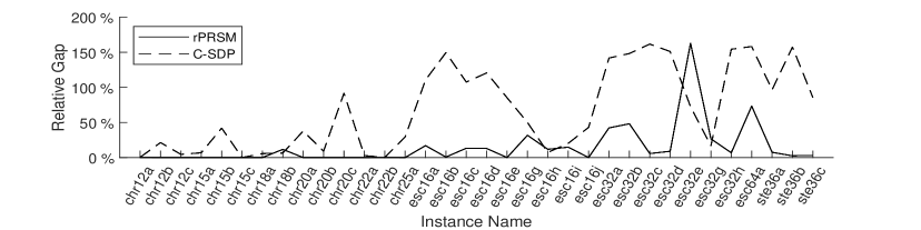
Figure 1: Relative Gap for rPRSM and C-SDP

The horizontal axis indicates the instance name on QAPLIB whereas the vertical axis indicates the relative gap. Figure 1 illustrates that rPRSM yields much stronger relative gaps than C-SDP.

Comparison to F2-RLT2-DA(​​​[9])

Date and Nagi [9] propose F2-RLT2-DA, a linearization technique-based parallel algorithm (GPU-based) for obtaining lower bounds via Lagrangian relaxation.

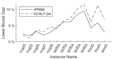
(a) Lower Bound Gap

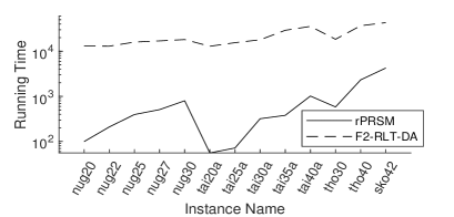
(b) Running Time

Figure 2: Numerical Comparison for rPRSM and F2-RLT2-DA

Figure 2(a) illustrates the comparisons on lower bound gap using rPRSM and F2-RLT2-DA. It shows that both rPRSM and F2-RLT2-DA output competitive lower bounds to the best known feasible values for QAP. Figure 2(b) illustrates the comparisons on the running time in seconds using rPRSM and F2-RLT2-DA. We observe that the running time of F2-RLT2-DA is much longer than the running time of rPRSM; F2-RLT2-DA requires at least 10 times longer than rPRSM. Furthermore, from Figure 2 we observe that even though the two methods give similar lower bounds to QAP, rPRSM is less time-consuming even considering the differences in the hardware.

5 Conclusion

In this paper we re-examin the strength of using a splitting method for solving the facially reduced SDP relaxation for the QAP with nonnegativity constraints added, that is, the splitting of constraints into two subproblems that are challenging to solve when used together. In addition, we provide a straightforward derivation of facial reduction and the gangster constraints via a direct lifting.

We use a strengthened model and algorithm, i.e., we incorporate a redundant trace constraint to the model that is not redundant in the subproblem from the splitting. We also exploit the set of dual optimal multipliers and provide customized dual updates in the algorithm that allow for a proof of optimality for the original QAP. This allowed for a new strategy for strengthening the upper and lower bounds.

References

• [1] A.F. Anjos and J.B. Lasserre, editors. Handbook on Semidefinite, Conic and Polynomial Optimization. International Series in Operations Research & Management Science. Springer-Verlag, 2011.
• [2] K.M. Anstreicher and N.W. Brixius. Solving quadratic assignment problems using convex quadratic programming relaxations. Technical report, University of Iowa, Iowa City, IA, 2000.
• [3] M. Bashiri and H. Karimi. Effective heuristics and meta-heuristics for the quadratic assignment problem with tuned parameters and analytical comparisons. Journal of Industrial Engineering International, 8(1):6, 2012.
• [4] R.K. Bhati and A. Rasool. Quadratic assignment problem and its relevance to the real world: A survey. International Journal of Computer Applications, 96(9):42–47, 2014.
• [5] G. Birkoff. Tres observaciones sobre el algebra lineal. Univ. Nac. Tucuman Rev., Ser. A:147–151, 1946.
• [6] J.F.S. Bravo Ferreira, Y. Khoo, and A. Singer. Semidefinite programming approach for the quadratic assignment problem with a sparse graph. Comput. Optim. Appl., 69(3):677–712, 2018.
• [7] E. Çela. The quadratic assignment problem, volume 1 of Combinatorial Optimization. Kluwer Academic Publishers, Dordrecht, 1998. Theory and algorithms.
• [8] Y. Chen and X. Ye. Projection onto a simplex. arXiv preprint arXiv:1101.6081, 2011.
• [9] K. Date and R. Nagi. Level 2 reformulation linearization technique-based parallel algorithms for solving large quadratic assignment problems on graphics processing unit clusters. INFORMS J. Comput., 31(4):771–789, 2019.
• [10] Z. Drezner. A new genetic algorithm for the quadratic assignment problem. INFORMS J. Comput., 15(3):320–330, 2003.
• [11] D. Drusvyatskiy and H. Wolkowicz. The many faces of degeneracy in conic optimization. Foundations and Trends® in Optimization, 3(2):77–170, 2017.
• [12] C. S. Edwards. The derivation of a greedy approximator for the koopmans-beckmann quadratic assignment problem. In Proceedings CP77 Combinatorial Prog. Conf., Liverpool, pages 55–86, 1977.
• [13] A.N. Elshafei. Hospital layout as a quadratic assignment problem. Operations Research Quarterly, 28:167–179, 1977.
• [14] L.M. Gambardella, É.D Taillard, and M. Dorigo. Ant colonies for the quadratic assignment problem. Journal of the operational research society, 50(2):167–176, 1999.
• [15] M. R. Garey and D. S. Johnson. Computers and Intractability. W. H. Freeman and Company, San Francisco, 1979.
• [16] A.M. Geoffrion and G.W. Graves. Scheduling parallel production lines with changeover costs: Practical applications of a quadratic assignment/LP approach. Operations Research, 24:595–610, 1976.
• [17] M.X. Goemans and D.P. Williamson. Improved approximation algorithms for maximum cut and satisfiability problems using semidefinite programming. J. Assoc. Comput. Mach., 42(6):1115–1145, 1995.
• [18] Y. Gu, B. Jiang, and D. Han. A semi-proximal-based strictly contractive Peaceman-Rachford splitting method. arXiv e-prints, page arXiv:1506.02221, Jun 2015.
• [19] B. He, H. Liu, Z. Wang, and X. Yuan. A strictly contractive peaceman–rachford splitting method for convex programming. SIAM Journal on Optimization, 24(3):1011–1040, 2014.
• [20] D.R Heffley. Assigning runners to a relay team. In Optimal strategies in sports, volume 5, pages 169–171. North Holland Amsterdam, 1977.
• [21] J. Krarup and P.M. Pruzan. Computer-aided layout design. In Mathematical programming in use, pages 75–94. Springer, 1978.
• [22] X. Li and X. Yuan. A proximal strictly contractive Peaceman-Rachford splitting method for convex programming with applications to imaging. SIAM J. Imaging Sci., 8(2):1332–1365, 2015.
• [23] J.E. Mitchell, P.M. Pardalos, and M.G.C Resende. Interior point methods for combinatorial optimization. In Handbook of combinatorial optimization, pages 189–297. Springer, 1998.
• [24] D.E. Oliveira, H. Wolkowicz, and Y. Xu. ADMM for the SDP relaxation of the QAP. Math. Program. Comput., 10(4):631–658, 2018.
• [25] P. Pardalos, F. Rendl, and H. Wolkowicz. The quadratic assignment problem: a survey and recent developments. In P.M. Pardalos and H. Wolkowicz, editors, Quadratic assignment and related problems (New Brunswick, NJ, 1993), pages 1–42. Amer. Math. Soc., Providence, RI, 1994.
• [26] P. Pardalos and H. Wolkowicz, editors. Quadratic assignment and related problems. American Mathematical Society, Providence, RI, 1994. Papers from the workshop held at Rutgers University, New Brunswick, New Jersey, May 20–21, 1993.
• [27] F. Rendl and R. Sotirov. Bounds for the quadratic assignment problem using the bundle method. Math. Program., 109(2-3, Ser. B):505–524, 2007.
• [28] R.T. Rockafellar. Convex analysis. Princeton Landmarks in Mathematics. Princeton University Press, Princeton, NJ, 1997. Reprint of the 1970 original, Princeton Paperbacks.
• [29] I. Ugi, J. Bauer, J. Brandt, J. Friedrich, J. Gasteiger, C. Jochum, and W. Schubert. Neue anwendungsgebiete für computer in der chemie. Angewandte Chemie, 91(2):99–111, 1979.
• [30] E. van den Berg and M.P. Friedlander. Probing the Pareto frontier for basis pursuit solutions. SIAM J. Sci. Comput., 31(2):890–912, 2008/09.
• [31] J. von Neumann. A certain zero-sum two-person game equivalent to the optimal assignment problem. In Contributions to the theory of games, vol. 2, Annals of Mathematics Studies, no. 28, pages 5–12. Princeton University Press, Princeton, N. J., 1953.
• [32] H. Wolkowicz, R. Saigal, and L. Vandenberghe, editors. Handbook of semidefinite programming. International Series in Operations Research & Management Science, 27. Kluwer Academic Publishers, Boston, MA, 2000. Theory, algorithms, and applications.
• [33] Q. Zhao, S.E. Karisch, F. Rendl, and H. Wolkowicz. Semidefinite programming relaxations for the quadratic assignment problem. volume 2, pages 71–109. 1998. Semidefinite programming and interior-point approaches for combinatorial optimization problems (Toronto, ON, 1996).