Two-parton scattering amplitudes in the Regge limit to high loop orders

Abstract

We study two-to-two parton scattering amplitudes in the high-energy limit of perturbative QCD by iteratively solving the BFKL equation. This allows us to predict the imaginary part of the amplitude to leading-logarithmic order for arbitrary $t$-channel colour exchange. The corrections we compute correspond to ladder diagrams with any number of rungs formed between two Reggeized gluons. Our approach exploits a separation of the two-Reggeon wavefunction, performed directly in momentum space, between a soft region and a generic (hard) region. The former component of the wavefunction leads to infrared divergences in the amplitude and is therefore computed in dimensional regularization; the latter is computed directly in two transverse dimensions and is expressed in terms of single-valued harmonic polylogarithms of uniform weight. By combining the two we determine exactly both infrared-divergent and finite contributions to the two-to-two scattering amplitude order-by-order in perturbation theory. We study the result numerically to 13 loops and find that finite corrections to the amplitude have a finite radius of convergence which depends on the colour representation of the $t$-channel exchange.

1 Introduction

The study of QCD scattering in the Regge limit has been an active area of research for over half a century, e.g. Kuraev:1977fs ; Balitsky:1978ic ; Lipatov:1985uk ; Mueller:1993rr ; Mueller:1994jq ; Brower:2006ea ; Moult:2017xpp . While the general problem of high-energy scattering is non-perturbative, in the regime where the exchanged momentum $-t$ is high enough, i.e. $s\gg-t\gg\Lambda_{\rm QCD}^{2}$ (see figure 1), perturbation theory offers systematic tools to analyse this limit. Central to this is the Balitsky-Fadin-Kuraev-Lipatov (BFKL) evolution equation Kuraev:1977fs ; Balitsky:1978ic , which provides a systematic theoretical framework to resum high-energy (or rapidity) logarithms, $\ln(s/(-t))$, to all orders in perturbation theory. This approach was used extensively to study a range of physical phenomena including the small-$x$ behaviour of deep-inelastic structure functions and parton densities, and jet production with large rapidity gaps. Furthermore, non-linear generalisations of BFKL, known as the Balitsky-JIMWLK equation Balitsky:1995ub ; Balitsky:1998kc ; Kovchegov:1999yj ; JalilianMarian:1996xn ; JalilianMarian:1997gr ; Iancu:2001ad , are today a main tool in the theoretical description of dense states of nuclear matter, notably in the context of heavy-ion collisions.

While many applications of rapidity evolution equations to phenomenology require the scattering particles to be colour-singlet objects, in the present paper we are concerned with the more theoretical problem of understanding partonic scattering amplitudes in the high-energy limit, similarly to refs. Sotiropoulos:1993rd ; Korchemsky:1993hr ; Korchemskaya:1996je ; Korchemskaya:1994qp ; DelDuca:2001gu ; DelDuca:2013ara ; DelDuca:2014cya ; Bret:2011xm ; DelDuca:2011ae ; Caron-Huot:2013fea ; Caron-Huot:2017fxr ; Caron-Huot:2017zfo . This is part of a more general programme of understanding the structure of gauge-theory amplitudes and the underlying physical and mathematical principles governing this structure. The basic observation is that gauge dynamics drastically simplifies in the high-energy limit, which renders the amplitudes computable to all orders in perturbation theory, to a given logarithmic accuracy.

The present paper continues our recent study Caron-Huot:2013fea ; Caron-Huot:2017fxr ; Caron-Huot:2017zfo of $2\to 2$ partonic amplitudes ($qq\to qq$, $gg\to gg$, $qg\to qg$) in QCD and related gauge theories.

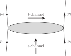
Figure 1: The $t$-channel exchange dominating the high-energy limit, $s\gg-t>0$. The figure also defines our conventions for momenta assignment and Mandelstam invariants. We shall assume that particles 2 and 3 (1 and 4) are of the same type and have the same helicity.

A key ingredient in these studies is provided once again by rapidity evolution equations, BFKL and its generalisations, which are used to compute high-energy logarithms in these amplitudes order-by-order in perturbation theory.

Scattering amplitudes of quarks and gluons are dominated at high energies by the $t$-channel exchange (figure 1) of effective degrees of freedom called Reggeized gluons. $2\to 2$ amplitudes are conveniently decomposed into odd and even signature characterising their symmetry properties under $s\leftrightarrow u$ interchange, or crossing symmetry:

$${\cal M}^{(\pm)}(s,t)=\tfrac{1}{2}\Big{(}{\cal M}(s,t)\pm{\cal M}(-s-t,t)\Big{)}\,,$$ (1)

where odd (even) amplitudes ${\cal M}^{(-)}$ (${\cal M}^{(+)}$) are governed by the exchange of an odd (even) number of Reggeized gluons. Furthermore, as shown in ref. Caron-Huot:2017fxr , these have respectively real and imaginary coefficients, when expressed in terms of the natural signature-even combination of logarithms,

$$\frac{1}{2}\left(\log\frac{-s-i0}{-t}+\log\frac{-u-i0}{-t}\right)\simeq\log\left|\frac{s}{t}\right|-i\frac{\pi}{2}\equiv L\,.$$ (2)

The real part of the amplitude, ${\cal M}^{(-)}$, is governed, at leading logarithmic (LL) accuracy, by the exchange of a single Reggeized gluon in the $t$ channel. To this accuracy, high-energy logarithms admit a simple exponentiation pattern, namely

$${\cal M}^{(-)}_{\rm LL}=(s/(-t))^{\alpha_{g}(t)}\times{\cal M}^{\rm tree}$$ (3)

where the exponent is the gluon Regge trajectory (corresponding to a Regge pole in the complex angular momentum plane), $\alpha_{g}(t)=\frac{\alpha_{s}}{\pi}C_{A}\alpha_{g}^{(1)}(t)+{\cal O}(\alpha_{s}^{2})$, whose leading order coefficient $\alpha_{g}^{(1)}(t)$ is infrared singular, $\alpha_{g}^{(1)}(t)\sim\frac{1}{2\epsilon}$ in dimensional regularization with $d=4-2\epsilon$ (see eq. (7) below). Infrared singularities are well-known to exponentiate, independently of the high-energy limit. Importantly, however, eq. (3) illustrates the fact that the exponentiation high-energy logarithms must be compatible with that of infrared singularities, which is a nontrivial constraint on both. This observation and its extension to higher logarithmic accuracy underpins a long line of investigation in refs. Sotiropoulos:1993rd ; Korchemsky:1993hr ; Korchemskaya:1996je ; Korchemskaya:1994qp ; DelDuca:2001gu ; DelDuca:2013ara ; DelDuca:2014cya ; Bret:2011xm ; DelDuca:2011ae ; Caron-Huot:2013fea ; Caron-Huot:2017fxr ; Caron-Huot:2017zfo .

The key property of the Reggeized gluon being signature-odd greatly constrains the structure of higher-order corrections. For the real part of amplitude, the simple exponentiation pattern generated by a single Reggeized gluon is preserved at the next-to-leading logarithmic (NLL) accuracy, except that it requires ${\cal O}(\alpha_{s}^{2})$ corrections to the trajectory and also the introduction of ($s$-independent) impact factors. This simple picture only breaks down when three Reggeized gluons can be exchanged, which first occurs at NNLL accuracy and leads to Regge cuts. This contribution was computed in ref. Caron-Huot:2017fxr through three-loops, by constructing an iterative solution of the non-linear Balitsky-JIMWLK equation which tested the mixing between one and three Reggeized gluons.

In this paper we focus on the imaginary part of the amplitude, ${\cal M}^{(+)}$, extending our work Caron-Huot:2017zfo . Here the leading tower of logarithms, in which we are interested, is generated by the exchange of two Reggeized gluons, starting with a non-logarithmic term at one loop:

$${\cal M}^{(+)}_{\rm NLL}\simeq i\pi\left[\frac{1}{2\epsilon}\frac{\alpha_{s}}{\pi}+{\cal O}\left(\alpha_{s}^{2}L\right)\right]{\mathbf{T}}^{2}_{s-u}{\cal M}^{\rm tree}\,.$$ (4)

Here we suppressed subleading terms in $\epsilon$ as well as multiloop corrections, which take the form $\alpha_{s}^{\ell}L^{\ell-1}$ at $\ell$ loops; because the power of the energy logarithm $L$ is one less than that of the coupling, these are formally next-to-leading logarithms (NLL). In eq. (4) one may observe another salient feature of this tower of corrections, namely the colour structure, which is even under $s\leftrightarrow u$ interchange (${\cal M}^{\rm tree}$ is odd, and so is the operator ${\mathbf{T}}^{2}_{s-u}$ acting on it). The first term in the square brackets in (4) is the exact result in the planar limit; we will be interested in the full series of corrections $\alpha_{s}^{\ell}L^{\ell-1}$, which are all subleading in the large $N_{c}$ limit (see the definitions of colour operators in eq. (12) below).

All higher-order corrections, ${\cal O}(\alpha_{s}^{\ell}L^{\ell-1})$, in (4) can be described by the well-known ladder graphs, where each additional loop constitute an additional rung in the ladder (see figure 2 below).

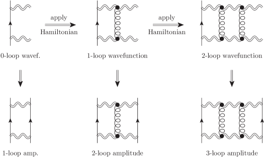
Figure 2: Sketch of bfkl evolution generating ladder graphs in the imaginary part of the amplitude. Considering initially emission from the projectile side only, the 0-loop wavefunction (top left) describes a state involving two reggeized gluons. The Reggeized gluons are both off-shell and are characterized by their transverse momenta $k$ and $p-k$. Each application of the BFKL Hamiltonian (the top row) generates an additional rung in the ladder. Upon integrating the $(\ell-1)$-loop wavefunction with the target one obtains the $\ell$-loop amplitude (bottom row).

Being the leading contributions to the imaginary part of the amplitude, they are particularly important, and clearly at high energies, where $\alpha_{s}L\sim{\cal O}(1)$, one should aim at an all-order calculation. These corrections, however, do not feature a simple exponentiation pattern as in eq. (3); they give rise to a Regge cut rather than a pole. We shall study these corrections using an iterative solution of the BFKL equation, continuing the work of ref. Caron-Huot:2013fea ; Caron-Huot:2017fxr ; Caron-Huot:2017zfo . In Caron-Huot:2013fea higher-order terms in eq. (4) were computed through four loops – the first order where finite contributions appear (see eqs. (28-29) in Caron-Huot:2017fxr ). Subsequently, in ref. Caron-Huot:2017zfo infrared-singular contributions were computed in dimensional regularization to all orders. The purpose of the present paper is to extend the calculation to finite contributions, and in particular, to obtain the infrared-renormalized amplitude, or hard function, which we expect (together with the soft anomalous dimension) to control any infrared-safe cross section.

We are interested in the exact perturbative solution of the BFKL equation for any colour exchange, that is, not restricted to the planar limit. While the BFKL Hamiltonian was famously diagonalized by its authors in the case of color-singlet exchange, the solution is not known in the general case. Adding to the complexity is the fact that amplitudes are infrared singular, forcing us to work in dimensional regularization. While it is not known how to diagonalise the BFKL Hamiltonian in these circumstances, we are able to solve the problem by using two complementary approaches, the first by taking the soft approximation while maintaining dimensional regularization, and the second by considering general (hard) kinematics in strictly two transverse dimensions. Let us briefly describe each of these approaches.

The first approach is a computation of the wavefunction describing the emission of two Reggeons at $(\ell-1)$ loops, and the corresponding $\ell$-loop $2\to 2$ amplitude, in the soft approximation, where one of the two Reggeized gluons carries transverse momentum $k^{2}$ which is significantly smaller than the total momentum transfer by the pair, $-t=p^{2}$, i.e. the limit characterized by a double hierarchy of scales $k^{2}\ll p^{2}\ll s$. This is the limit used in ref. Caron-Huot:2017zfo to determine all infrared-singular contributions the amplitude. This was achieved using the simple observation that the wavefunction is itself finite to all orders in perturbation theory and that BFKL evolution closes within this approximation. All the singularities of the amplitude at any given loop order are in turn produced in the final integration over the wavefunction (corresponding to the transition from the top to the bottom row in figure 2). In the present paper, building upon the computation of the wavefunction in Caron-Huot:2017zfo we introduce a symmetrized solution accounting simultaneously for the two soft limits, $k^{2}\ll p^{2}$ and $(p-k)^{2}\ll p^{2}$, which amounts to an elegant separation between soft and hard contributions to the wavefunction and amplitude. Within this approximation we are able to write down a resummed analytic expression for the amplitude, including its finite contributions.

The second approach, which we develop in the present paper, is based on starting with the BFKL equation in exactly two dimensions. Without making any further approximation, we set up an iterative solution of the equation by identifying differential operators that commute with (parts of) the Hamiltonian up to a computable set of contact terms. Evolution induced by the Hamiltonian then becomes trivial within a class of iterated integrals dictated by the nature of the problem, these are the Single-Valued Harmonic Polylogarithms (SVHPLs), first systematically classified by Francis Brown in ref. Brown:2004ugm and then studied and applied in the context of motivic periods Brown:2013gia and Feynman integrals Chavez:2012kn ; Schnetz:2013hqa . The relevance of this class of functions for gauge-theory amplitudes within the Regge limit Pennington:2012zj ; Dixon:2012yy ; DelDuca:2013lma ; Dixon:2014voa ; DelDuca:2016lad ; DelDuca:2018hrv (and beyond Almelid:2017qju ; Dixon:2019lnw ) has been recognised in recent years, and it is important also in our current problem: the hard wavefunction, defined in strictly two dimensions, is fully expressible in terms of SVHPLs, and the corresponding contribution to the amplitude can in turn be written in terms of Single-Valued Multiple Zeta Values (SVMZVs). For the ladder graphs relevant here, each additional loop increases the transcendental weight by one unit. The resulting uniform-weight expressions in terms of single-valued functions are significantly simpler as compared to the corresponding ones in terms of ordinary polylogarithms and zeta values. For the final integration over the wavefunction we develop two independent approaches, one relying on analytic continuation and integration over the discontinuities of the wavefunction away from the region were they are single-valued, and the other relying instead on a modified application of the evolution algorithm itself. The two yield identical results. By combining the hard contribution to the amplitude with the dimensional-regularized soft contribution we compute the full amplitude, in principle to any order, and in practice to thirteen loops.

The structure of the paper is as follows. In section 2 we present the BFKL equation in dimensional regularisation, bring it to a form suitable for iterative solution and review the relation between the off-shell wavefunction and the two-to-two scattering amplitude. We also show how an iterative solution can be obtained for the first few orders directly in dimensional regularization without resorting to any approximation, and explain why this approach does not practically extend to higher orders. In this context we compute the amplitude numerically through five loops, providing a valuable check for our subsequent calculations. Next, in section 3 we review the soft approximation developed in Caron-Huot:2017zfo and explain how infrared factorization, combined with the finiteness of the wavefunction, facilitate a systematic separation of the latter into ‘soft’ and ‘hard’ components, such that eventually, finite corrections to the infrared-renormalized scattering amplitude can be determined in full. To this end we introduce a symmetrized version of the soft wavefunction, which captures both soft limits, and then derive an analytic expression for the amplitude as a function of $\alpha_{s}L$, which resums both infrared-divergent and finite contributions to all loops, within the soft approximation. In section 4 we turn to discuss the wavefunction in general (hard) kinematics. Working directly in two dimensions we introduce the relevant kinematic variables, analyse the action of the BFKL Hamiltonian and demonstrate that evolution generated by this Hamiltonian translates into an algorithmic procedure in the space of SVHPLs. Having determined the wavefunction order by order, we turn in section 5 to compute the corresponding two-to-two scattering amplitude. In section 6 we perform a numerical study of the resulting wavefunctions and amplitudes, and address the convergence of the perturbative expansion. Finally, in section 7 we make some concluding comments and present an outlook for future investigation.

2 bfkl equation in dimensional regularisation and the $2\to 2$ amplitude

In the high-energy limit, scattering amplitudes are conveniently described in terms of Wilson lines, which dress the external partons. The evaluation of vacuum expectation values of Wilson lines stretching from minus to plus infinity leads to rapidity divergences, which needs to be renormalised. As a consequence, the renormalised amplitude obeys a rapidity evolution equation, which can be shown to correspond to the Balitsky-JIMWLK equation. In this paper we are interested to study the two-Reggeon exchange contribution to two-parton scattering amplitudes, for which the evolution equation reduces to the BFKL equation Caron-Huot:2013fea ; Caron-Huot:2017fxr . The scattering amplitude can be determined formally to any order in perturbation theory as an iterative solution of the dimensionally-regularised BFKL equation. This procedure was described in Caron-Huot:2017zfo , to which we refer for further details. In this section we review the definitions necessary to set up the calculation.

In the following we consider the two-reggeon exchange contribution to $2\to 2$ scattering amplitudes. We can single out this contribution by introducing a reduced amplitude, in which the one-Reggeon exchange has been removed:

$$\hat{\mathcal{M}}_{ij\to ij}\equiv e^{-\alpha_{g}(t)L\mathbf{T}_{t}^{2}}\mathcal{M}_{ij\to ij},$$ (5)

where $L$ is the signature-even high-energy logarithm defined in eq. (2), $\mathbf{T}_{t}^{2}$ represents the total colour charge exchanged in the $t$ channel (see eq. (12) below) and $i,j$ are the species indices defining the two-parton scattering; in what follows we will drop these indices, unless explicitly needed. Finally, the function

$$\alpha_{g}(t)=\frac{\alpha_{s}}{\pi}\alpha_{g}^{(1)}(t)+{\cal O}(\alpha_{s}^{2})$$ (6)

is the gluon Regge trajectory introduced already in eq. (3), where the leading-order coefficient in dimensional regularization with $d=4-2\epsilon$ is given by

$$\alpha_{g}^{(1)}(t)=\frac{B_{0}}{2\epsilon}\left(\frac{-t}{\mu^{2}}\right)^{-\epsilon}$$ (7)

where

$$B_{0}\equiv B_{0}(\epsilon)=e^{\epsilon\gamma_{\rm E}}\frac{\Gamma^{2}(1-\epsilon)\Gamma(1+\epsilon)}{\Gamma(1-2\epsilon)}=1-\frac{1}{2}\epsilon^{2}\zeta_{2}-\frac{7}{3}\epsilon^{3}\zeta_{3}+O(\epsilon^{4})$$ (8)

belongs to a class of bubble integrals which will be defined below.

The two-Reggeon cut contributes only to the even amplitude defined in eq. (1), thus we focus only on this component in the following. As discussed in Caron-Huot:2017zfo , the reduced amplitude takes the form of an integral over the two-Reggeon wavefunction $\Omega(p,k)$, as follows:

$$\hat{\mathcal{M}}_{\mathrm{NLL}}^{(+)}\left(\frac{s}{-t}\right)=-i\pi\int[\mathrm{D}k]\frac{p^{2}}{k^{2}(p-k)^{2}}\,\Omega(p,k)\,\mathbf{T}_{s-u}^{2}\,\mathcal{M}^{\mathrm{(tree)}}_{ij\to ij},$$ (9)

where $p^{2}=-t$. In eq. (9) the integration measure is

$$[\mathrm{D}k]\equiv\frac{\pi}{B_{0}}\left(\frac{\mu^{2}}{4\pi e^{-\gamma_{\mathrm{E}}}}\right)^{\epsilon}\frac{\mathrm{d}^{2-2\epsilon}k}{(2\pi)^{2-2\epsilon}},$$ (10)

and $\mathcal{M}^{\mathrm{(tree)}}_{ij\to ij}$ represent the tree amplitude, given by

$$\mathcal{M}^{\mathrm{(tree)}}_{ij\to ij}=4\pi\alpha_{s}\frac{2s}{t}(T_{i}^{b})_{a_{1}a_{4}}(T_{j}^{b})_{a_{2}a_{3}}\delta_{\lambda_{1}\lambda_{4}}\delta_{\lambda_{2}\lambda_{3}},$$ (11)

where $\lambda_{i}$ for $i=1$ through $4$ are helicity indices. The colour operator $\mathbf{T}_{s-u}^{2}$ in eq. (9) acts on $\mathcal{M}^{\mathrm{(tree)}}_{ij\to ij}$ and it is defined in terms of the usual basis of quadratic Casimirs corresponding to colour flow through the three channels Dokshitzer:2005ig ; DelDuca:2011ae :

$$\mathbf{T}_{s-u}^{2}\equiv\frac{\mathbf{T}_{s}^{2}-\mathbf{T}_{u}^{2}}{2}\qquad\rm{with}\qquad\left\{\begin{array}[]{c}\mathbf{T}_{s}=\mathbf{T}_{1}+\mathbf{T}_{2}=-\mathbf{T}_{3}-\mathbf{T}_{4},\\ \mathbf{T}_{u}=\mathbf{T}_{1}+\mathbf{T}_{3}=-\mathbf{T}_{2}-\mathbf{T}_{4},\\ \mathbf{T}_{t}=\mathbf{T}_{1}+\mathbf{T}_{4}=-\mathbf{T}_{2}-\mathbf{T}_{3},\end{array}\right.$$ (12)

where $\mathbf{T}_{i}$ is the colour-charge operator Catani:1998bh associated with parton $i$.

The BFKL equation Kuraev:1977fs ; Balitsky:1978ic for the wavefunction $\Omega(p,k)$ in eq. (9) takes the form

$$\frac{d}{dL}\Omega(p,k)=\frac{\alpha_{s}B_{0}(\epsilon)}{\pi}\hat{H}\Omega(p,k)\,,$$ (13)

where $L$ is the high-energy logarithm (2) and where the Hamiltonian takes the form Caron-Huot:2017zfo

$$\hat{H}=(2C_{A}-\mathbf{T}_{t}^{2})\,\hat{H}_{\mathrm{i}}+(C_{A}-\mathbf{T}_{t}^{2})\,\hat{H}_{\mathrm{m}},$$ (14)

where two independent colour factors come along with two different operations:

$$\hat{H}_{\mathrm{i}}\,\Psi(p,k) =\int[\mathrm{D}k^{\prime}]\,f(p,k,k^{\prime})\left[\Psi(p,k^{\prime})-\Psi(p,k)\right],$$ (15a)

$$\hat{H}_{\mathrm{m}}\,\Psi(p,k) =J(p,k)\,\Psi(p,k)\,\,.$$ (15b)

The function $f(p,k,k^{\prime})$ in eq. (15a) represents the bfkl evolution kernel

$$f(p,k,k^{\prime})\equiv\frac{k^{2}}{(k^{\prime})^{2}(k-k^{\prime})^{2}}+\frac{(p-k)^{2}}{(p-k^{\prime})^{2}(k-k^{\prime})^{2}}-\frac{p^{2}}{(k^{\prime})^{2}(p-k^{\prime})^{2}}\,,$$ (16)

and $J(p,k)$ in eq. (15b) is defined by

$$J(p,k)=\frac{1}{2\epsilon}+\int[\mathrm{D}k^{\prime}]\,f(p,k,k^{\prime})=\frac{1}{2\epsilon}\left[2-\left(\frac{p^{2}}{k^{2}}\right)^{\epsilon}-\left(\frac{p^{2}}{(p-k)^{2}}\right)^{\epsilon}\right].$$ (17)

While it is unknown how to diagonalise this $d$-dimensional Hamiltonian, we may invoke a perturbative solution Caron-Huot:2013fea ; Caron-Huot:2017zfo by expanding the wavefunction in the strong coupling constant:

$$\Omega(p,k) = \sum_{\ell=1}^{\infty}\left(\frac{\alpha_{s}}{\pi}\right)^{\ell}L^{\ell-1}\frac{B_{0}^{\ell}}{(\ell-1)!}\,\Omega^{({\ell-1})}(p,k),$$ (18)

where we set the renormalisation scale equal to the momentum transfer, $\mu^{2}=-t=p^{2}$.

Substituting the expanded form of the wavefunction in (18) into the BFKL evolution equation (13) one deduces that

$$\Omega^{({\ell-1})}(p,k)=\hat{H}\Omega^{({\ell-2})}(p,k),$$ (19)

where $\hat{H}$ is the BFKL hamiltonian of eq. (14), that is, the wavefunction at any given order is found by repeated application of the bfkl Hamiltonian, where the initial condition in our normalization is simply

$$\Omega^{({0})}(p,k)=1\,\,.$$ (20)

Next, let us consider the on-shell $2\to 2$ amplitude. Substituting the expanded wavefunction (18) into (9) we readily obtain the following expansion

$$\hat{\mathcal{M}}_{\mathrm{NLL}}^{(+)}\left(\frac{s}{-t}\right) = \sum_{\ell=1}^{\infty}\left(\frac{\alpha_{s}}{\pi}\right)^{\ell}L^{\ell-1}\,\hat{\mathcal{M}}_{\mathrm{NLL}}^{(+,{\ell})},$$ (21)

with

$$\hat{\mathcal{M}}_{\mathrm{NLL}}^{(+,{\ell})}=-i\pi\frac{B_{0}^{\ell}}{(\ell-1)!}\int[\mathrm{D}k]\frac{p^{2}}{k^{2}(p-k)^{2}}\Omega^{({\ell-1})}(p,k)\mathbf{T}_{s-u}^{2}\mathcal{M}^{\mathrm{(tree)}}\,.$$ (22)

Namely, integrating over the $(\ell-1)$-th order contribution to the wavefunction yields the $\ell$-th order contribution to the amplitude.

A graphical illustration of eq. (22) is provided in figure 3. As discussed in the introduction, because of bfkl evolution, the amplitude at nll accuracy can be represented as a ladder. At order $\ell$ it is obtained by closing the ladder and integrating the wavefunction of order $(\ell-1)$ over the resulting loop momentum, according to eq. (22). The wavefunction $\Omega^{({\ell-1})}(p,k)$ in turn is obtained by applying once the leading-order bfkl evolution kernel to the wavefunction of order $(\ell-2)$. Graphically, this operation corresponds to adding one rung to the ladder.

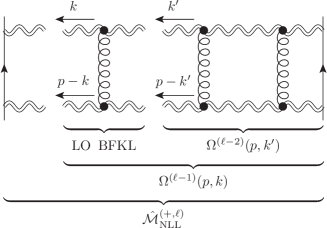
Figure 3: Graphical representation of the amplitude at nll accuracy, as obtained through bfkl evolution. The addition of one rung corresponds to applying once the leading-order bfkl evolution on the wavefunction of order $(\ell-2)$. This gives the wavefunction at order $(\ell-1)$, according to eq. (14). Closing the ladder and integrating over the resulting loop momentum gives the reduced amplitude, according to eq. (22).

Inspecting eqs. (15a) and (15b) we see that the BFKL evolution consists of an integration and a multiplication part. The effect of evolution is thus expressed formally in a compact form by introducing a class of functions

$$\Omega_{\mathrm{i},w}(p,k) \equiv\int[\mathrm{D}k^{\prime}]f(p,k,k^{\prime})\left[\Omega_{w}(p,k^{\prime})-\Omega_{w}(p,k)\right],$$ (23a)

$$\Omega_{\mathrm{m},w}(p,k) \equiv J(p,k)\,\Omega_{w}(p,k),$$ (23b)

where $\Omega_{\varnothing}(p,k)\equiv 1$, and $w$ indicates a word made of indices “i” or “m”, which stand for integration and multiplication, respectively, according to the action of the two Hamiltonian operators in eq. (15a) and (15b), respectively. In this notation the first four orders of the wavefunction read, for instance,

$$\Omega^{({1})}(p,k) =(C_{A}-\mathbf{T}_{t}^{2})\Omega_{\rm m},$$ (24)

$$\Omega^{({2})}(p,k) =(C_{A}-\mathbf{T}_{t}^{2})^{2}\Omega_{\rm m,m}+(2C_{A}-\mathbf{T}_{t}^{2})(C_{A}-\mathbf{T}_{t}^{2})\Omega_{\rm i,m},$$ (25)

$$\Omega^{({3})}(p,k) =(C_{A}-\mathbf{T}_{t}^{2})^{3}\Omega_{\rm m,m,m}+(2C_{A}-\mathbf{T}_{t}^{2})(C_{A}-\mathbf{T}_{t}^{2})^{2}\left(\Omega_{\rm i,m,m}+\Omega_{\rm m,i,m}\right)$$

$$+\,(2C_{A}-\mathbf{T}_{t}^{2})^{2}(C_{A}-\mathbf{T}_{t}^{2})\Omega_{\rm i,i,m},$$ (26)

$$\Omega^{({4})}(p,k) =(C_{A}-\mathbf{T}_{t}^{2})^{4}\Omega_{\rm m,m,m,m}$$

$$+\,(2C_{A}-\mathbf{T}_{t}^{2})(C_{A}-\mathbf{T}_{t}^{2})^{3}\left(\Omega_{\rm m,m,i,m}+\Omega_{\rm m,i,m,m}+\Omega_{\rm i,m,m,m}\right)$$

$$+\,(2C_{A}-\mathbf{T}_{t}^{2})^{2}(C_{A}-\mathbf{T}_{t}^{2})^{2}\left(\Omega_{\rm m,i,i,m}+\Omega_{\rm i,m,i,m}+\Omega_{\rm i,i,m,m}\right)$$

$$+\,(2C_{A}-\mathbf{T}_{t}^{2})^{3}(C_{A}-\mathbf{T}_{t}^{2})\Omega_{\rm i,i,i,m}.$$ (27)

Symmetries play an important role in determining the general structure of the wavefunction, and from a practical perspective they can be useful to reduce the number of integrals that need to be evaluated at each loop order. The wavefunction is symmetric under swapping the two $t$-channel Reggeons, which can be understood from the graphical representation of the bfkl evolution in figure 3. This implies

$$\Omega^{({\ell})}(p,k)=\Omega^{({\ell})}(p,p-k)\,,$$ (28)

which can be easily verified by showing that the functions $f(p,k,k^{\prime})$ in (16), $J(p,k)$ in (17) and $\Omega^{({0})}(p,k)$ in (20) obey the same symmetry. This symmetry property will become handy in section 3, making it possible to capture simultaneously both soft limits, $k^{2}\to 0$ and $(p-k)^{2}\to 0$. This, in turn, will be important for implementing a systematic separation between the soft and hard regimes, without needing an extra regulator.

Despite the simplifications allowed by symmetries, though, the evaluation of the wavefunction in $2-2\epsilon$ transverse dimensions without additional simplifications becomes quickly infeasible. For instance, already the wavefunctions with one or two integrations (one or two occurrences of the index “i”) involve integrals of the type

$$\Omega_{\rm i,m} \ni\int[\mathrm{D}k^{\prime}]\,\frac{(p-k)^{2}}{(p-k^{\prime})^{2}(k-k^{\prime})^{2}}\left(\frac{p^{2}}{(k^{\prime})^{2}}\right)^{\epsilon},$$

$$\Omega_{\rm i,i,m} \ni\int[\mathrm{D}k^{\prime}][Dk^{\prime\prime}]\,\frac{k^{2}(p-k^{\prime\prime})^{2}}{(k^{\prime\prime})^{2}(p-k^{\prime})^{2}(k-k^{\prime\prime})^{2}(k^{\prime}-k^{\prime\prime})^{2}}\left(\frac{p^{2}}{(k^{\prime})^{2}}\right)^{\epsilon},$$ (29)

which are represented respectively in figure 4 (a) and (b). Such integrals evaluates to Appell, and more in general Lauricella functions in dimensional regularisation. Given the lack of a systematic classification of these functions in terms of iterated integrals, the evaluation of the wavefunction beyond the third order is not practical.

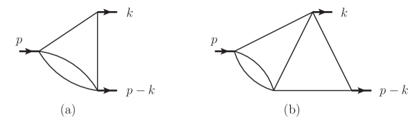
Figure 4: Three-mass triangle integrals with massless propagators, which appear in the calculation of the wavefunction at two and three loops. These integrals contribute to the amplitude only starting respectively at four and five loops, due to symmetry constraints, as discussed in the main text. The bubble integral on one of the edges of the triangle clarifies the origin of the propagator which is raised to power $\epsilon$ in eq. (2).

The amplitude at order $\ell$ is obtained upon integrating the wavefunction of order $\ell-1$, as indicated in eq. (22). As in case of the wavefunction, symmetries turn out to be important for a simplification of the calculation and interpretation of the result. While the two Reggeons in the wavefunction can be defined to originate from either the projectile or target Wilson line — which gives the corresponding ladder graphs a sense of direction — this is no longer true at the level of the amplitude. Physically the two cases become indistinguishable, and we refer to this as the target-projectile symmetry. In general, this implies the relation Caron-Huot:2017zfo

$$\int[\mathrm{D}k]\frac{p^{2}}{k^{2}(p-k)^{2}}\hat{H}_{\mathrm{i}}\Omega_{w}(p,k)=\int[\mathrm{D}k]\frac{p^{2}}{k^{2}(p-k)^{2}}\Omega_{\mathrm{i},w}(p,k)=0.$$ (30)

Furthermore, in the notation of eqs. (23a) and (23b) reversal of the rungs directly translates to the reversal of the indices of the wavefunction. The target-projectile symmetry thus guarantees the equality

$$\int[\mathrm{D}k]\frac{p^{2}}{k^{2}(p-k)^{2}}\Omega_{a_{1},\dots,a_{n}}(p,k)=\int[\mathrm{D}k]\frac{p^{2}}{k^{2}(p-k)^{2}}\Omega_{a_{n},\dots,a_{1}}(p,k).$$ (31)

The symmetries discussed above can reduce the number of functions to be computed significantly, and make the calculation of the amplitude trivial up to three loops, since it can be shown that the integration of the wavefunction involves only bubble integrals. Furthermore, the calculation of the amplitude at four loops in dimensional regularisation is still feasible, as it involve bubble integrals and a single more involved kite-like integral, represented in figure 5 (a). Up to four loops one obtains Caron-Huot:2017zfo

$$\hat{\mathcal{M}}_{\mathrm{NLL}}^{(+,{1})} =i\pi\frac{B_{0}}{2\epsilon}\mathbf{T}_{s-u}^{2}\mathcal{M}^{\mathrm{(tree)}},$$ (32)

$$\hat{\mathcal{M}}_{\mathrm{NLL}}^{(+,{2})} =i\pi\frac{(B_{0})^{2}}{2}\left[\frac{1}{(2\epsilon)^{2}}+\frac{9\zeta_{3}}{2}\epsilon+\frac{27\zeta_{4}}{4}\epsilon^{2}+\frac{63\zeta_{5}}{2}\epsilon^{3}+\mathcal{O}(\epsilon^{4})\right]$$

$$\hskip 156.49014pt\times(C_{A}-\mathbf{T}_{t}^{2})\mathbf{T}_{s-u}^{2}\mathcal{M}^{\mathrm{(tree)}},$$ (33)

$$\hat{\mathcal{M}}_{\mathrm{NLL}}^{(+,{3})} =i\pi\frac{B_{0}^{3}}{3!}\left[\frac{1}{(2\epsilon)^{3}}-\frac{11\zeta_{3}}{4}-\frac{33\zeta_{4}}{8}\epsilon-\frac{357\zeta_{5}}{4}\epsilon^{2}+\mathcal{O}(\epsilon^{3})\right]$$

$$\hskip 156.49014pt\times(C_{A}-\mathbf{T}_{t}^{2})^{2}\mathbf{T}_{s-u}^{2}\mathcal{M}^{\mathrm{(tree)}},$$ (34)

$$\hat{\mathcal{M}}_{\mathrm{NLL}}^{(+,{4})} =i\pi\frac{B_{0}^{4}}{4!}\bigg{\{}(C_{A}-\mathbf{T}_{t}^{2})^{3}\left(\frac{1}{(2\epsilon)^{4}}+\frac{175\zeta_{5}}{2}\epsilon+\mathcal{O}(\epsilon^{2})\right)$$

$$\hskip 22.76219pt+C_{A}(C_{A}-\mathbf{T}_{t}^{2})^{2}\left(-\frac{\zeta_{3}}{8\epsilon}-\frac{3}{16}\zeta_{4}-\frac{167\zeta_{5}}{8}\epsilon+\mathcal{O}(\epsilon^{2})\right)\bigg{\}}\mathbf{T}_{s-u}^{2}\mathcal{M}^{\mathrm{(tree)}}.$$ (35)

A thorough discussion of the target-projectile symmetry, and its effect on the colour structure of the amplitude has been given in Caron-Huot:2017zfo , to which we refer for further details. In this paper we are interested to evaluate the amplitude, including finite terms, to higher orders in the perturbative expansion. Despite the symmetries discussed above, however, beyond four loops the iterated integrals appearing are all but easy with current methods.

A simple and fast way to extend the study in ref. Caron-Huot:2013fea ; Caron-Huot:2017zfo to higher loops is provided by numerical integration methods. In particular, we find sector decomposition as implemented in pySecDec/SecDec Carter:2010hi ; Borowka:2017esm to be suited to calculate the nested integrals that enter the five-loop amplitude. Provided a high numerical accuracy it is straightforward to extract from the results the rational coefficients of the zeta numbers appearing at this loop order. This procedure relies on the observed homogeneous transcendental weight property of the $\ell$-loop amplitude: Assigning $o(\epsilon)=-1$, $o(\pi)=1$ and $o(\zeta_{n})=n$ one sees that the terms of the $\ell$-loop amplitude are uniformly of weight $o(\hat{\mathcal{M}}_{\mathrm{NLL}}^{(+,{\ell})})=\ell$. We can hence deduce which zeta numbers (or powers of $\pi$) may appear at any given order in $\epsilon$.

Another observation facilitates this procedure at five loops; after dividing the $\ell$-loop amplitude by $B_{0}^{\ell}$ (8) there are no occurrences of $\zeta_{2}=\pi^{2}/6$ up to four loops, see e.g. the $\mathcal{O}(\epsilon)$ terms of eq. (2). If we assume this absence of $\zeta_{2}$ to be an actual property of the amplitude, the finite terms of the five-loop amplitude can only be proportional to one transcendental number, $\zeta_{5}$, whereas $\zeta_{3}\zeta_{2}$ is excluded. At this point this approach may seem rather conjectural. However, over the course of the next two sections we develop methods that prove this assumption, and we shall briefly return to it at the end of section 5.3.

To obtain the five-loop amplitude $\hat{\mathcal{M}}_{\mathrm{NLL}}^{(+,{5})}$ we integrate the four-loop wavefunction $\Omega^{({4})}(p,k)$ of (27) according to eq. (22). In doing so one is faced with a plethora of multi-loop integrals. Many of them correspond to bubble graphs and can be easily evaluated analytically. Others vanish because of the symmetries discussed above. The remaining integrals can be computed numerically using pySecDec. One of the more difficult examples is shown in figure 5. In the depicted case one can integrate out the two internal bubbles and is left with a three-loop integral with two of the propagators raised to non-integer powers:

$$\text{figure~{}\ref{fig:5loopex} (b)}\sim\int\frac{[\mathrm{D}k][\mathrm{D}k^{\prime}][\mathrm{D}k^{\prime\prime}]\,(p-k^{\prime})^{2}}{(k^{2})^{\epsilon}(k^{\prime})^{2}((k^{\prime\prime})^{2})^{\epsilon}(k-k^{\prime})^{2}(k^{\prime}-k^{\prime\prime})^{2}(p-k)^{2}(p-k^{\prime\prime})^{2}}.$$ (36)

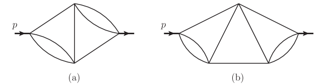
Figure 5: Example of a four- and five-loop integrals that enters the calculation of the four- and five-loop amplitude respectively. The two bubbles may be integrated out, turning it into a two- and three-loop integral with two propagators raised to non-integer powers, cf. eq. (36).

After combining all contributions (and reconstructing the zeta numbers in case of the numerical results) we find

$$\hat{\mathcal{M}}_{\mathrm{NLL}}^{(+,{5})}=i\pi\frac{B_{0}^{5}}{5!}\left\{(C_{A}-\mathbf{T}_{t}^{2})^{4}\left(\frac{1}{32\epsilon^{5}}-\frac{53\zeta_{5}}{2}\right)\right.\\ \left.+C_{A}(C_{A}-\mathbf{T}_{t}^{2})^{3}\left(-\frac{\zeta_{3}}{16\epsilon^{2}}-\frac{3\zeta_{4}}{32\epsilon}+\frac{253\zeta_{5}}{16}\right)-\frac{5}{2}C_{A}^{2}(C_{A}-\mathbf{T}_{t}^{2})^{2}\zeta_{5}\right\}\mathbf{T}_{s-u}^{2}\mathcal{M}^{\mathrm{(tree)}}.$$ (37)

This result will serve as a consistency check for our computation below.

3 The soft approximation

In section 2 we have shown how the two-Reggeon contribution to the two-parton scattering amplitude is conveniently described in terms of the reduced amplitude $\hat{\cal M}$. The latter is defined in eq. (5) by (multiplicatively) removing the single-Reggeon effect from the full amplitude ${\cal M}$. This allowed us to use BFKL evolution to express the two-Reggeon contribution to $\hat{\cal M}$ in terms of iterated integrals. Beyond four loops these integrals become difficult to evaluate exactly in $d=4-2\epsilon$ dimensions, but as we are going to show now, this is also not necessary.

Ultimately we are interested in extracting physical information about the scattering process, and dimensional regularization is used in the present context for the sole purpose of regularizing long-distance singularities. Here infrared factorization come into play: the long-distance singularities of ${\cal M}$ can be factorized, ${\cal M}={\bf Z}\mathcal{H}$, where the “infrared renormalization” factor ${\bf Z}$ captures all divergences (which famously exponentiate in terms of the soft anomalous dimension, see e.g. Sterman:1995fz ; Collins:1989gx ; Korchemskaya:1994qp ; Catani:1998bh ; Aybat:2006mz ; Sterman:2002qn ; Gardi:2009qi ; Becher:2009cu ; Becher:2009qa ; Almelid:2015jia ; Almelid:2017qju ) while the infrared-renormalized amplitude $\mathcal{H}$ – sometimes referred to as the “hard function” – is finite, and can be evaluated in four space-time dimensions (or equivalently, two transverse dimensions). To understand this from a physical perspective recall that physical quantities such as cross sections are finite: starting from the infrared-singular amplitude ${\cal M}$, their calculation inevitably incorporates a mechanism of cancellation of the singularities involving soft real-gluon emission. Once this was implemented, the finite, physical result can only depend on four-dimensional quantities, namely the soft anomalous dimension and the infrared-renormalized amplitude $\mathcal{H}$.

In Ref. Caron-Huot:2017zfo we have shown that the soft anomalous dimension associated with the signature-even amplitude, or indeed the relevant infrared renormalization factor ${\bf Z}$, can be computed to all orders by evaluating the reduced amplitude $\hat{\mathcal{M}}$ to $\mathcal{O}(\epsilon^{-1})$. Similarly, we are going to show now (section 3.1) that the infrared-renormalized amplitude $\mathcal{H}$ (in four dimensions) can be completely determined from the reduced amplitude $\hat{\mathcal{M}}$, evaluated at the same accuracy, i.e. to $\mathcal{O}(\epsilon^{0})$. This, along with the fact that the corresponding wavefunction $\Omega$ is finite, greatly simplifies the task of performing BFKL evolution to high loop orders, because it allows us to follow an “expansion by region” approach: in section 3.2 we split the wavefunction into soft and hard components, each of which is rendered computable using different considerations. The soft wavefunction – giving rise to all the singularities in the amplitude – can be computed analytically in dimensional regularization owing to the drastic simplification of BFKL evolution in this limit, while the hard wavefunction is only required in strictly two transverse dimensions, where BFKL evolution again simplifies (see section 4). These two wavefunction components will subsequently serve to compute the corresponding soft and hard contributions to the reduced amplitude $\hat{\mathcal{M}}$ to the required order, $\mathcal{O}(\epsilon^{0})$. In section 3.3 we review the main results of Ref. Caron-Huot:2017zfo regarding the all-order computation of the wavefunction within the soft approximation. We also introduce there a symmetrized soft wavefunction which captures both soft limits. This, in turn, is used in section 3.4 to compute the corresponding $\mathcal{O}(\epsilon^{0})$ contributions to the reduced amplitude. Finally, in section 3.5 we make use of the results of sections 3.1 and 3.4 to evaluate the $\mathcal{O}(\epsilon^{0})$ soft contributions to the infrared-renormalized amplitude $\mathcal{H}$.

3.1 Infrared factorisation in the high-energy limit

According to the infrared factorisation theorem (see e.g. Sterman:1995fz ; Collins:1989gx ; Korchemskaya:1994qp ; Catani:1998bh ; Aybat:2006mz ; Sterman:2002qn ; Gardi:2009qi ; Becher:2009cu ; Becher:2009qa ; Almelid:2015jia ; Almelid:2017qju ), infrared singularities of an amplitude $\mathcal{M}$ are multiplicatively renormalised by a factor ${\bf Z}$,

$$\mathcal{M}\left(\{p_{i}\},\mu,\alpha_{s}(\mu)\right)\,=\,{\bf Z}\left(\{p_{i}\},\mu,\alpha_{s}(\mu)\right)\mathcal{H}\left(\{p_{i}\},\mu,\alpha_{s}(\mu)\right)\,,$$ (38)

such that the infrared-renormalized amplitude ${\cal H}$ is finite as $\epsilon\to 0$. We use a minimal subtraction scheme, where the renormalisation factor ${\bf Z}$ consists of pure poles. It is then given explicitly as the path-ordered exponential of the soft anomalous dimension:

$${\bf Z}\left(\{p_{i}\},\mu,\alpha_{s}(\mu)\right)\,=\,{\cal P}\exp\left\{-\int_{0}^{\mu}\frac{d\lambda}{\lambda}\,{\bf\Gamma}\left(\{p_{i}\},\lambda,\alpha_{s}(\lambda)\right)\right\},$$ (39)

where, to the accuracy needed in this paper, we can restrict to tree-level running coupling: $\alpha_{s}(\lambda)=\alpha_{s}(p)\left(p^{2}/\lambda^{2}\right)^{\epsilon}$. Given that ${\bf Z}$ was determined in Ref. Caron-Huot:2017zfo to NLL accuracy in the high-energy logarithm, our goal here is to determine the infrared-renormalized amplitude ${\cal H}$ to the same accuracy. Thus we need to specialise eq. (38) to the high-energy limit. Recalling that in this limit the amplitude splits naturally into even and odd components under the $s\leftrightarrow u$ signature symmetry, we may focus directly on the even component (the odd component was analysed already in Caron-Huot:2017fxr ):

$$\mathcal{M}^{(+)}_{\rm NLL}={\bf Z}^{(-)}_{\rm NLL}\,\mathcal{H}^{(-)}_{\rm LL}+{\bf Z}^{(+)}_{\rm LL}\,\mathcal{H}^{(+)}_{\rm NLL}.$$ (40)

Our final goal is to determine $\mathcal{H}^{(+)}_{\rm NLL}$. Let us begin by inverting (40), i.e.

$$\mathcal{H}^{(+)}_{\rm NLL}=-\big{(}{\bf Z}^{-1}\big{)}^{(+)}_{\rm LL}{\bf Z}^{(-)}_{\rm NLL}\,\mathcal{H}^{(-)}_{\rm LL}+\big{(}{\bf Z}^{-1}\big{)}^{(+)}_{\rm LL}\mathcal{M}^{(+)}_{\rm NLL}.$$ (41)

In eq. (41) both the leading- and next-to-leading logarithmic renormalisation factors are known: ${\bf Z}^{(+)}_{\rm LL}$, and hence also $\big{(}{\bf Z}^{-1}\big{)}^{(+)}_{\rm LL}$ is easily determined from the single-Reggeon exchange, see eqs. (3) and (7):

$${\bf Z}^{(+)}_{\rm LL}=e^{\frac{x}{2\epsilon}\mathbf{T}_{t}^{2}}\,\qquad\quad\Longrightarrow\qquad\quad\big{(}{\bf Z}^{-1}\big{)}^{(+)}_{\rm LL}=e^{-\frac{x}{2\epsilon}\mathbf{T}_{t}^{2}}\,,$$ (42)

where we defined $x\equiv\frac{\alpha_{s}}{\pi}L$. The factor ${\bf Z}^{(-)}_{\rm NLL}$ was determined to all orders in perturbation theory in Caron-Huot:2017zfo : comparing eqs. (4.12), (4.14) and (4.17) there we express ${\bf Z}^{(-)}_{\rm NLL}$ as

$$e^{-\frac{x}{2\epsilon}\mathbf{T}_{t}^{2}}\,{\bf Z}^{(-)}_{\rm NLL}=i\pi\,\frac{e^{\frac{x}{2\epsilon}(C_{A}-\mathbf{T}_{t}^{2})}-1}{L(C_{A}-\mathbf{T}_{t}^{2})}\left(1-\frac{C_{A}}{C_{A}-\mathbf{T}_{t}^{2}}R(\epsilon)\right)^{-1}\mathbf{T}_{s-u}^{2}\Bigg{|}_{\rm poles},$$ (43)

where the function $R(\epsilon)$ reads

$$R(\epsilon) = \frac{\Gamma^{3}(1-\epsilon)\Gamma(1+\epsilon)}{\Gamma(1-2\epsilon)}-1$$ (44)

$$= -2\zeta_{3}\,\epsilon^{3}-3\zeta_{4}\,\epsilon^{4}-6\zeta_{5}\epsilon^{5}-\left(10\zeta_{6}-2\zeta^{2}_{3}\right)\epsilon^{6}+{\cal O}(\epsilon^{7}),$$

see also eq. (3.16) of Caron-Huot:2017zfo . In eq. (43) the factor $\exp[-(x\mathbf{T}_{t}^{2})/(2\epsilon)]$ on the l.h.s. is left there, because it corresponds directly to the factor $\big{(}{\bf Z}^{-1}\big{)}^{(+)}_{\rm LL}$ appearing in eq. (41) to the left of ${\bf Z}^{(-)}_{\rm NLL}$. Notice also that the $-1$ in the numerator of the first fraction on the r.h.s. of eq. (43) can actually be removed, given that we need to consider only the poles originating from eq. (43), and this term contributes only at $\mathcal{O}(\epsilon^{0})$, given that the second $\epsilon$-dependent factor is regular, i.e. $\big{[}1-C_{A}/(C_{A}-\mathbf{T}_{t}^{2})\,R(\epsilon)\big{]}^{-1}=1+\mathcal{O}(\epsilon^{3})$.

Eq. (41) contains also the leading-logarithmic infrared-renormalized amplitude $\mathcal{H}^{(-)}_{\rm LL}$, which, as in case of ${\bf Z}^{(+)}_{\rm LL}$, is determined by single-Reggeon exchange, compare again with eqs. (3) and (7):

$$\mathcal{H}^{(-)}_{\rm LL}=e^{\frac{B_{0}(\epsilon)-1}{2\epsilon}\,x\,C_{A}}\mathcal{M}^{\rm(tree)}\,,$$ (45)

where we have substituted $\mathbf{T}_{t}^{2}\to C_{A}$, given that in $\mathcal{H}^{(-)}_{\rm LL}$ the operator $\mathbf{T}_{t}^{2}$ acts on the tree-level amplitude.

By this point we collected all ingredients needed to explicitly write down the first term in eq. (41). The only missing term on the r.h.s. of this equation is thus the even amplitude itself, $\mathcal{M}^{(+)}_{\rm NLL}$. As explained above, in order to determine $\mathcal{M}^{(+)}_{\rm NLL}$ by means of BFKL evolution, we wish to express it in terms of the reduced amplitude ${\cal\hat{M}}^{(+)}_{\rm NLL}$ of eq. (5). Substituting eqs. (5), (42) and (45) into eq. (41) we get

$$\mathcal{H}^{(+)}_{\rm NLL}=-e^{-\frac{x}{2\epsilon}\mathbf{T}_{t}^{2}}{\bf Z}^{(-)}_{\rm NLL}\,e^{\frac{B_{0}(\epsilon)-1}{2\epsilon}\,x\,C_{A}}\mathcal{M}^{\rm(tree)}+e^{\frac{B_{0}(\epsilon)-1}{2\epsilon}\,x\,\mathbf{T}_{t}^{2}}{\cal\hat{M}}^{(+)}_{\rm NLL}\,\,,$$ (46)

where the factor $e^{-\frac{x}{2\epsilon}\mathbf{T}_{t}^{2}}{\bf Z}^{(-)}_{\rm NLL}$ of (43) can be readily substituted as well (this will be done in section 3.5). Eq. (46) is an important step because (given that $B_{0}(\epsilon)-1={\cal O}(\epsilon^{2})$, eq. (8)) it clearly shows that the hard function $\mathcal{H}^{(+)}_{\rm NLL}$ at $\epsilon\to 0$ is completely determined once the BFKL-motivated reduced amplitude ${\cal\hat{M}}^{(+)}_{\rm NLL}$ is known to $\mathcal{O}(\epsilon^{0})$, which is the result anticipated at the beginning of this section. With this in mind, we proceed to compute ${\cal\hat{M}}^{(+)}_{\rm NLL}$ to $\mathcal{O}(\epsilon^{0})$.

3.2 Soft and hard wavefunction and amplitude

Our strategy to compute the finite part of the reduced amplitude ${\cal\hat{M}}^{(+)}_{\rm NLL}$ at higher orders is to separate soft and hard components of the wavefunction and truncate the latter to two transverse dimensions ($\epsilon=0$), where BFKL evolution is much more tractable (see section 4).

As demonstrated in ref. Caron-Huot:2017zfo , the soft limit of the wavefunction, where one of the two Reggeons has a small momentum, e.g., $k^{2}\ll(p-k)^{2}\simeq p^{2}$, fully determines all the singular parts in $\epsilon$. This was used to obtain the all-order result for the renormalisation factor ${\bf Z}^{(-)}_{\rm NLL}$ in eq. (43). In addition, the soft limit generates some ${\cal O}(\epsilon^{0})$ finite contributions, which must be added to those generated by the complementary hard region, where both $k^{2}$ and $(p-k)^{2}$ are of order $p^{2}$.

To control ${\cal O}(\epsilon^{0})$ terms a clear separation between the two regions is necessary. We choose to do this at the level of the wavefunction $\Omega(p,q)$. Recall that $\Omega(p,q)$ is a finite function of $\epsilon$ Caron-Huot:2017zfo , i.e. any singularities in the reduced amplitude are generated through the final integration over the wavefunction in (9). To proceed we split the wavefunction into two terms:

$$\Omega(p,k)=\Omega_{\mathrm{s}}(p,k)+\Omega_{\mathrm{h}}(p,k)\,,$$ (47)

such that the second term, the hard component, vanishes in soft limits:

$$\lim_{k\to 0}\Omega_{\mathrm{h}}(p,k)=\lim_{k\to p}\Omega_{\mathrm{h}}(p,k)=0.$$ (48)

It then follows from (9) that no singularities can be generated upon integrating $\Omega_{\mathrm{h}}(p,k)$ (i.e. all the singularities in $\hat{\mathcal{M}}_{\mathrm{NLL}}^{(+)}$ are generated upon integrating $\Omega_{\mathrm{s}}(p,k)$) and hence only the $\epsilon\to 0$ limit of $\Omega_{\mathrm{h}}$ contributes to the finite part of the reduced amplitude. Denoting the wavefunction in this limit as

$$\Omega_{\mathrm{h}}^{({\rm 2d})}(p,k)\,\equiv\,\lim_{\epsilon\to 0}\Omega_{\mathrm{h}}=\Omega_{\mathrm{2d}}(p,k)-\Omega_{\mathrm{s}}^{({\rm 2d})}(p,k),$$ (49)

the reduced amplitude (9), through order ${\cal O}(\epsilon^{0})$, is then given as a sum of soft and hard components:

$$\hat{\mathcal{M}}_{\mathrm{NLL}}^{(+)}\left(\frac{s}{-t}\right)=\hat{\cal M}^{(+)}_{\rm NLL,s}\left(\frac{s}{-t}\right)+\hat{\cal M}^{(+)}_{\rm NLL,h}\left(\frac{s}{-t}\right)$$ (50)

with

$$\hat{\cal M}^{(+)}_{\rm NLL,s}\left(\frac{s}{-t}\right) =-i\pi\int[\mathrm{D}k]\,\frac{p^{2}}{k^{2}(p-k)^{2}}\Omega_{\mathrm{s}}(p,k)\,\,\mathbf{T}_{s-u}^{2}\mathcal{M}^{\mathrm{(tree)}}_{ij\to ij}\,,$$ (51a)

$$\hat{\cal M}^{(+)}_{\rm NLL,h}\left(\frac{s}{-t}\right) =-i\pi\lim_{\epsilon\to 0}\int[\mathrm{D}k]\,\frac{p^{2}}{k^{2}(p-k)^{2}}\,\Omega_{\mathrm{h}}^{({\rm 2d})}(p,k)\,\,\mathbf{T}_{s-u}^{2}\mathcal{M}^{\mathrm{(tree)}}_{ij\to ij}\,.$$ (51b)

Equations (50) and (51) are central to our approach and will guide our computations in what follows. They show that, to compute the finite part of the reduced amplitude, we must treat the soft wavefunction exactly as a function of $\epsilon$, but we are allowed to truncate the hard wavefunction to ${\cal O}(\epsilon^{0})$. Note that in (51b) we have already substituted the two-dimensional limit of the hard wavefunction, so taking the $\epsilon\to 0$ limit simply amounts to taking the integration momentum $k$ to be two-dimensional. These finite integrals will be done in section 5.

Let us briefly summarise our plan for the reminder of this section. After reviewing the main arguments of Caron-Huot:2017zfo , our aim in section 3.3 is to present a symmetrized version of the soft wavefunction in dimensional regularization, eq. (3.3), which simultaneously captures the two regions where either of the two Reggeons is soft. We then extract the ${\cal O}(\epsilon^{0})$ terms in the wavefunction and resum them; these will be used in section 5 to determine the two-dimensional hard wavefunction $\Omega_{\mathrm{h}}^{({\rm 2d})}(p,k)$ from the full one according to eq. (49). Subsequently in section 3.4 we use the soft wavefunction, computed to all-orders in $\epsilon$, to determine the corresponding contributions to the reduced $2\to 2$ amplitude. We also present an analytic formula resumming these corrections in eq. (73). Finally, in section 3.5 we determine the soft wavefunction contribution to the infrared-renormalized amplitude $\mathcal{H}^{(+)}_{\rm NLL}$ using eq. (46).

3.3 The soft wavefunction

The central property of the wavefunction $\Omega(p,k)$ highlighted in Caron-Huot:2017zfo and already mentioned above, is the fact that it is finite for $\epsilon\to 0$, to all orders in perturbation theory. This has far reaching consequences, because it means that all singularities in the amplitude must arise from the last integration in (9), and originate from the soft limits $k\to 0$ and $k\to p$ of $\Omega(p,k)$. One finds that it is particularly easy to calculate the wavefunction in these limits: as it turns out, the soft approximation is closed under BFKL evolution, i.e., starting with ${\Omega}^{(j)}(p,k)$, with $k$ soft, implies that the momentum $k^{\prime}$ in ${\Omega}^{(j-1)}(p,k^{\prime})$, which has one rung fewer, can also be taken soft, $k^{\prime}\to 0$, without affecting the result for ${\Omega}^{(j)}(p,k)$. In other words, starting with ${\Omega}^{(j)}(p,k)$ where $k$ is soft is equivalent to considering the entire side rail of the ladder consisting of soft momenta, $k^{\prime}$, $k^{\prime\prime}$, $\ldots\to 0$. Similarly, starting with $k\to p$ implies that all momenta $(p-k)$, $(p-k^{\prime})$, $(p-k^{\prime\prime})$, $\ldots$, are soft. The symmetry of eq. (28), then, implies that $\Omega(p,k)$ in the two limits $k\to 0$ and $k\to p$ must be the same.

In the soft limit the BFKL hamiltonian becomes Caron-Huot:2017zfo

$$\Omega^{(\ell-1)}_{s}(p,k) = \hat{H}_{s}\,\Omega^{(\ell-2)}_{s}(p,k)\,,$$

$$\hat{H}_{s}\Psi(p,k) = (2C_{A}-\mathbf{T}_{t}^{2})\int[Dk^{\prime}]\frac{2(k\cdot k^{\prime})}{k^{\prime 2}(k-k^{\prime})^{2}}\,\Big{[}\Psi(p,k^{\prime})-\Psi(p,k)\Big{]}$$ (52)

$$+\,(C_{A}-\mathbf{T}_{t}^{2})\,J_{s}(p,k)\,\Psi(p,k)\,,$$

where

$$J_{s}(p,k)=\frac{1}{2\epsilon}\left[1-\left(\frac{p^{2}}{k^{2}}\right)^{\epsilon}\,\right],$$ (53)

is the soft approximation of eq. (17). One finds that the wavefunction becomes a polynomial in $\xi\equiv(p^{2}/k^{2})^{\epsilon}$, i.e., the soft limit turns BFKL evolution into a one-scale problem. The integrals involved in eq. (52) are simple bubble integrals of the type

$$\int[{\rm D}k^{\prime}]\,\frac{2(k\cdot k^{\prime})}{k^{\prime 2}(k-k^{\prime})^{2}}\,\left(\frac{p^{2}}{k^{\prime 2}}\right)^{n\epsilon}=-\frac{1}{2\epsilon}\frac{B_{n}(\epsilon)}{B_{0}(\epsilon)}\left(\frac{p^{2}}{k^{2}}\right)^{(n+1)\epsilon}\,,$$ (54)

where the integration measure is given in eq. (10), and the class of bubble functions $B_{n}(\epsilon)$ is

$$B_{n}(\epsilon)=e^{\epsilon\gamma_{\rm E}}\frac{\Gamma(1-\epsilon)}{\Gamma(1+n\epsilon)}\frac{\Gamma(1+\epsilon+n\epsilon)\Gamma(1-\epsilon-n\epsilon)}{\Gamma(1-2\epsilon-n\epsilon)}\,.$$ (55)

Note that $B_{0}$ of (8) appearing in the gluon Regge trajectory and in the measure (10) corresponds to the special case of (55) with $n=0$.

Using eq. (54) one can write the action of the soft Hamiltonian (52) on any monomial ($m\geq 0$):

$$\hat{H}_{s}\,\xi^{m} = \frac{\xi^{m}}{2\epsilon}\left((1-\xi)(C_{A}-\mathbf{T}_{t}^{2})+\xi\hat{B}_{m}(\epsilon)(2C_{A}-\mathbf{T}_{t}^{2})\right)\,$$

$$= \frac{(C_{A}-\mathbf{T}_{t}^{2})}{2\epsilon}\left(\xi^{m}-\xi^{m+1}\left[1-\hat{B}_{m}(\epsilon)\frac{2C_{A}-\mathbf{T}_{t}^{2}}{C_{A}-\mathbf{T}_{t}^{2}}\right]\right)\,,$$

where we have introduced the notation

$$\hat{B}_{n}(\epsilon)\equiv 1-\frac{B_{n}(\epsilon)}{B_{0}(\epsilon)}\,=\,2n(2+n)\zeta_{3}\epsilon^{3}+3n(2+n)\zeta_{4}\epsilon^{4}+\ldots\,.$$ (57)

By making repeated use of eq. (3.3) one finds that the wavefunction at order $(\ell-1)$ can be expressed in a closed-form, as follows Caron-Huot:2017zfo :

$${\Omega}_{s}^{(\ell-1)}(p,k)=\frac{(C_{A}-\mathbf{T}_{t}^{2})^{\ell-1}}{(2\epsilon)^{\ell-1}}\sum_{n=0}^{\ell-1}(-1)^{n}\binom{\ell-1}{n}\left(\frac{p^{2}}{k^{2}}\right)^{n\epsilon}\prod_{m=0}^{n-1}\left\{1-\hat{B}_{m}(\epsilon)\frac{(2C_{A}-\mathbf{T}_{t}^{2})}{(C_{A}-\mathbf{T}_{t}^{2})}\right\}\,.$$ (58)

As discussed in Caron-Huot:2017zfo , this expression can be easily integrated, obtaining an expression for the amplitude which correctly describes its singular part to all orders in perturbation theory.

While eq. (58) is perfectly valid in the soft limit, it breaks explicitly the symmetry of eq. (28) between the two soft limits. As we will see below, it is advantageous to work with expressions where this symmetry is manifest. In this paper, we thus introduce a different soft wavefunction, obtained by symmetrising eq. (58) under $k\leftrightarrow(p-k)$:

$${\Omega}_{s}^{(\ell-1)}(p,k) =\frac{(C_{A}-\mathbf{T}_{t}^{2})^{\ell-1}}{(2\epsilon)^{\ell-1}}\sum_{n=0}^{\ell-1}(-1)^{n}\binom{\ell-1}{n}\left(\frac{p^{2}}{k^{2}}\right)^{n\epsilon}\bigg{(}\frac{p^{2}}{(p-k)^{2}}\bigg{)}^{n\epsilon}$$

$$\hskip 85.35826pt\times\,\prod_{m=0}^{n-1}\left\{1-\hat{B}_{m}(\epsilon)\frac{(2C_{A}-\mathbf{T}_{t}^{2})}{(C_{A}-\mathbf{T}_{t}^{2})}\right\}\,.$$ (59)

This formula simultaneously captures the correct behaviour of $\Omega(p,k)$ in both soft limits $k\to 0$ and $k\to p$. It will be used in section 3.4 below to compute the soft contributions to the reduced $2\to 2$ amplitude. Before doing that let us have a closer look at the $\epsilon$ expansion of the soft wavefunction we obtained.

We recall Caron-Huot:2017zfo that all the negative powers of $\epsilon$ in (3.3) cancel upon performing the sum over $n$, leading to a finite wavefunction at any loop order. While positive powers of $\epsilon$ in (3.3) do play a role in the computation of the amplitude, the leading $\mathcal{O}(\epsilon^{0})$ have a special role: according to eq. (49) it is precisely what must be subtracted from the full two-dimensional wavefunction to obtain the hard wavefunction $\Omega_{\mathrm{h}}^{({\rm 2d})}$. With this in mind, let us write down explicitly the leading terms in $\epsilon$ in the first few orders of the soft wavefunction in (3.3):

$$\Omega^{({0})}_{\mathrm{s}}(p,k)\big{|}_{\mathcal{O}(\epsilon^{0})} =0,$$ (60a)

$$\Omega^{({1})}_{\mathrm{s}}(p,k)\big{|}_{\mathcal{O}(\epsilon^{0})} =\frac{(C_{A}-\mathbf{T}_{t}^{2})}{2}\log\left(\frac{k^{2}(p-k)^{2}}{(p^{2})^{2}}\right),$$ (60b)

$$\Omega^{({2})}_{\mathrm{s}}(p,k)\big{|}_{\mathcal{O}(\epsilon^{0})} =\frac{(C_{A}-\mathbf{T}_{t}^{2})^{2}}{4}\log^{2}\left(\frac{k^{2}(p-k)^{2}}{(p^{2})^{2}}\right),$$ (60c)

$$\Omega^{({3})}_{\mathrm{s}}(p,k)\big{|}_{\mathcal{O}(\epsilon^{0})} =\frac{(C_{A}-\mathbf{T}_{t}^{2})^{3}}{8}\log^{3}\left(\frac{k^{2}(p-k)^{2}}{(p^{2})^{2}}\right)+\frac{(2C_{A}-\mathbf{T}_{t}^{2})(C_{A}-\mathbf{T}_{t}^{2})^{2}}{2}\zeta_{3},$$ (60d)

$$\Omega^{({4})}_{\mathrm{s}}(p,k)\big{|}_{\mathcal{O}(\epsilon^{0})} =\frac{(C_{A}-\mathbf{T}_{t}^{2})^{4}}{16}\log^{4}\left(\frac{k^{2}(p-k)^{2}}{(p^{2})^{2}}\right)$$

$$+\,(2C_{A}-\mathbf{T}_{t}^{2})(C_{A}-\mathbf{T}_{t}^{2})^{3}\log\left(\frac{k^{2}(p-k)^{2}}{(p^{2})^{2}}\right)\zeta_{3},$$ (60e)

$$\Omega^{({5})}_{\mathrm{s}}(p,k)\big{|}_{\mathcal{O}(\epsilon^{0})} =\frac{(C_{A}-\mathbf{T}_{t}^{2})^{5}}{32}\log^{5}\left(\frac{k^{2}(p-k)^{2}}{(p^{2})^{2}}\right)$$

$$+\,\frac{(2C_{A}-\mathbf{T}_{t}^{2})(C_{A}-\mathbf{T}_{t}^{2})^{4}}{4}\left[5\log^{2}\left(\frac{k^{2}(p-k)^{2}}{(p^{2})^{2}}\right)\zeta_{3}+6\zeta_{5}\right]\,.$$ (60f)

In fact, these terms exponentiate and can be resummed into the following all-order expression using (18) for $\epsilon=0$, yielding

$$\Omega_{\mathrm{s}}(p,k)\big{|}_{\mathcal{O}(\epsilon^{0})}=\frac{\alpha_{s}}{\pi}\left[e^{-x\gamma_{\mathrm{E}}(C_{A}-\mathbf{T}_{t}^{2})}\frac{\Gamma\left(1-\frac{x}{2}(C_{A}-\mathbf{T}_{t}^{2})\right)}{\Gamma\left(1+\frac{x}{2}(C_{A}-\mathbf{T}_{t}^{2})\right)}\right]^{\frac{2C_{A}-\mathbf{T}_{t}^{2}}{C_{A}-\mathbf{T}_{t}^{2}}}{\left(\frac{k^{2}(p-k)^{2}}{(p^{2})^{2}}\right)}^{\frac{x}{2}(C_{A}-\mathbf{T}_{t}^{2})},$$ (61)

with $x=L\,\alpha_{s}/\pi$.

3.4 Soft contributions to the $2\to 2$ amplitude

Next, let us consider the soft contribution to the reduced $2\to 2$ scattering amplitude $\hat{\cal M}$. It is straighforward to insert eq. (3.3) into eq. (22), perform the last integration and derive the $\ell$-th order contribution to the amplitude. In particular, given the symmetrised form of eq. (3.3), the last integration can be done with the integration measure $[{\rm D}k]$ in eq. (10), i.e. avoiding the need to introduce a cut-off as in ref. Caron-Huot:2017zfo . After some arrangement we get

$$\hat{\mathcal{M}}_{{\rm NLL,s}}^{(+,\ell)} = i\pi\,\frac{1}{(2\epsilon)^{\ell}}\,\frac{\left(B_{0}(\epsilon)\right)^{\ell}}{\ell!}\,\,(C_{A}-\mathbf{T}_{t}^{2})^{\ell-1}\sum_{n=1}^{\ell-1}(-1)^{n+1}\,\binom{\ell}{n}\frac{\tilde{B}_{n}(\epsilon)}{B_{0}(\epsilon)}$$ (62)

$$\hskip 85.35826pt\times\,\prod_{m=0}^{n-2}\bigg{[}1-\hat{B}_{m}(\epsilon)\frac{(2C_{A}-\mathbf{T}_{t}^{2})}{(C_{A}-\mathbf{T}_{t}^{2})}\bigg{]}\,\mathbf{T}_{s-u}^{2}\,\mathcal{M}^{\mathrm{(tree)}},$$

where the functions $B_{n}(\epsilon)$ and $\hat{B}_{n}(\epsilon)$ have been defined respectively in eqs. (55) and (57), and we have introduced

$$\tilde{B}_{n}(\epsilon)=e^{\epsilon\gamma_{E}}\frac{\Gamma^{2}\big{(}1-n\epsilon\big{)}\Gamma\big{(}1-\epsilon+2n\epsilon\big{)}}{\Gamma\big{(}1-2n\epsilon\big{)}\Gamma^{2}\big{(}1-\epsilon+n\epsilon\big{)}}.$$ (63)

The coefficients $\hat{\mathcal{M}}_{{\rm NLL,s}}^{(+,\ell)}$ in (62) are of course polynomial in the colour factors. For illustration, we expand eq. (62) to the first few orders in perturbation theory, obtaining

$$\hat{\mathcal{M}}_{\rm NLL,s}^{(1)} =i\pi B_{0}\bigg{\{}\frac{1}{2\epsilon}\bigg{\}}\mathbf{T}_{s-u}^{2}\mathcal{M}^{\mathrm{(tree)}},$$ (64a)

$$\hat{\mathcal{M}}_{\rm NLL,s}^{(2)} =i\pi\frac{B_{0}^{2}}{2}\bigg{\{}\frac{C_{2}}{4\epsilon^{2}}\bigg{\}}\mathbf{T}_{s-u}^{2}\mathcal{M}^{\mathrm{(tree)}},$$ (64b)

$$\hat{\mathcal{M}}_{\rm NLL,s}^{(3)} =i\pi\frac{B_{0}^{3}}{3!}\bigg{\{}C_{2}^{2}\left(\frac{1}{8\epsilon^{3}}-\frac{11\zeta_{3}}{4}\right)-C_{1}C_{2}\frac{3\zeta_{3}}{4}\bigg{\}}\mathbf{T}_{s-u}^{2}\mathcal{M}^{\mathrm{(tree)}},$$ (64c)

$$\hat{\mathcal{M}}_{\rm NLL,s}^{(4)} =i\pi\frac{B_{0}^{4}}{4!}\bigg{\{}C_{2}^{3}\left(\frac{1}{16\epsilon^{4}}+\frac{\zeta_{3}}{8\epsilon}+\frac{3\zeta_{4}}{16}\right)+C_{1}C_{2}^{2}\left(-\frac{\zeta_{3}}{8\epsilon}-\frac{3\zeta_{4}}{16}\right)\bigg{\}}\mathbf{T}_{s-u}^{2}\mathcal{M}^{\mathrm{(tree)}},$$ (64d)

$$\hat{\mathcal{M}}_{\rm NLL,s}^{(5)} =i\pi\frac{B_{0}^{5}}{5!}\bigg{\{}C_{2}^{4}\left(\frac{1}{32\epsilon^{5}}+\frac{\zeta_{3}}{16\epsilon^{2}}+\frac{3\zeta_{4}}{32\epsilon}-\frac{717\zeta_{5}}{16}\right)$$

$$\hskip 28.45274pt+\,C_{1}C_{2}^{3}\left(-\frac{\zeta_{3}}{16\epsilon^{2}}-\frac{3\zeta_{4}}{32\epsilon}-\frac{27\zeta_{5}}{16}\right)\bigg{\}}\mathbf{T}_{s-u}^{2}\mathcal{M}^{\mathrm{(tree)}},$$ (64e)

$$\hat{\mathcal{M}}_{\rm NLL,s}^{(6)} =i\pi\frac{B_{0}^{6}}{6!}\bigg{\{}C_{1}^{2}C_{2}^{3}\bigg{(}-\frac{39\zeta_{3}^{2}}{16}\bigg{)}+C_{1}C_{2}^{4}\bigg{(}-\frac{\zeta_{3}}{32\epsilon^{3}}-\frac{3\zeta_{4}}{64\epsilon^{2}}-\frac{3\zeta_{5}}{32\epsilon}-\frac{963\zeta_{3}^{2}}{32}+\frac{5\zeta_{6}}{32}\bigg{)}$$

$$\hskip 28.45274pt+C_{2}^{5}\bigg{(}\frac{1}{64\epsilon^{6}}+\frac{\zeta_{3}}{32\epsilon^{3}}+\frac{3\zeta_{4}}{64\epsilon^{2}}+\frac{3\zeta_{5}}{32\epsilon}-\frac{2879\zeta_{3}^{2}}{32}+\frac{5\zeta_{6}}{32}\bigg{)}\bigg{\}}\mathbf{T}_{s-u}^{2}\mathcal{M}^{\mathrm{(tree)}},$$ (64f)

$$\hat{\mathcal{M}}_{\rm NLL,s}^{(7)} =i\pi\frac{B_{0}^{7}}{7!}\bigg{\{}C_{1}^{2}C_{2}^{4}\bigg{(}\frac{\zeta_{3}^{2}}{32\epsilon}+\frac{3\zeta_{3}\zeta_{4}}{32}\bigg{)}+C_{1}C_{2}^{5}\bigg{(}-\frac{\zeta_{3}}{64\epsilon^{4}}-\frac{3\zeta_{4}}{128\epsilon^{3}}-\frac{3\zeta_{5}}{64\epsilon^{2}}$$

$$\hskip 28.45274pt-\,\frac{3\zeta_{3}^{2}}{64\epsilon}-\frac{5\zeta_{6}}{64\epsilon}-\frac{9\zeta_{3}\zeta_{4}}{64}-\frac{729\zeta_{7}}{64}\bigg{)}+C_{2}^{6}\bigg{(}\frac{1}{128\epsilon^{7}}+\frac{\zeta_{3}}{64\epsilon^{4}}+\frac{3\zeta_{4}}{128\epsilon^{3}}+\frac{3\zeta_{5}}{64\epsilon^{2}}$$

$$\hskip 28.45274pt+\,\frac{\zeta_{3}^{2}}{64\epsilon}+\frac{5\zeta_{6}}{64\epsilon}+\frac{3\zeta_{3}\zeta_{4}}{64}-\frac{90711\zeta_{7}}{64}\bigg{)}\bigg{\}}\mathbf{T}_{s-u}^{2}\mathcal{M}^{\mathrm{(tree)}},$$ (64g)

$$\hat{\mathcal{M}}_{\rm NLL,s}^{(8)} =i\pi\frac{B_{0}^{8}}{8!}\bigg{\{}C_{1}^{2}C_{2}^{5}\bigg{(}\frac{\zeta_{3}^{2}}{64\epsilon^{2}}+\frac{3\zeta_{3}\zeta_{4}}{64\epsilon}-\frac{1341\zeta_{3}\zeta_{5}}{32}+\frac{21\zeta_{8}}{512}\bigg{)}+C_{1}C_{2}^{6}\bigg{(}-\frac{\zeta_{3}}{128\epsilon^{5}}$$

$$\hskip 28.45274pt-\,\frac{3\zeta_{4}}{256\epsilon^{4}}-\frac{3\zeta_{5}}{128\epsilon^{3}}-\frac{3\zeta_{3}^{2}}{128\epsilon^{2}}-\frac{5\zeta_{6}}{128\epsilon^{2}}-\frac{9\zeta_{3}\zeta_{4}}{128\epsilon}-\frac{9\zeta_{7}}{128\epsilon}-\frac{96777\zeta_{3}\zeta_{5}}{64}$$

$$\hskip 28.45274pt-\,\frac{189\zeta_{8}}{1024}\bigg{)}+C_{2}^{7}\bigg{(}\frac{1}{256\epsilon^{8}}+\frac{\zeta_{3}}{128\epsilon^{5}}+\frac{3\zeta_{4}}{256\epsilon^{4}}+\frac{3\zeta_{5}}{128\epsilon^{3}}+\frac{\zeta_{3}^{2}}{128\epsilon^{2}}+\frac{5\zeta_{6}}{128\epsilon^{2}}$$

$$\hskip 28.45274pt+\frac{3\zeta_{3}\zeta_{4}}{128\epsilon}+\frac{9\zeta_{7}}{128\epsilon}-\frac{483837\zeta_{3}\zeta_{5}}{64}+\frac{147\zeta_{8}}{1024}\bigg{)}\bigg{\}}\mathbf{T}_{s-u}^{2}\mathcal{M}^{\mathrm{(tree)}}\,,$$ (64h)

where we used the shorthand notation for the colour factors, $C_{1}=(2C_{A}-\mathbf{T}_{t}^{2})$ and $C_{2}=(C_{A}-\mathbf{T}_{t}^{2})$. We note that the expansion coefficients display uniform transcendental weight (where, as usual $1/\epsilon$ has weight 1) and involve exclusively single zeta values (sometimes referred to as ordinary zeta values, namely the values of the Riemann zeta function at integer arguments). We further notice that $\zeta_{2}$ (or $\zeta_{2}$ times other zeta values, e.g. $\zeta_{2}\zeta_{3}$ at weight 5, etc.) factors do not appear in eqs. (64a)–(64) ($\zeta_{2}$ terms would be present if we were to expand the factor factor $B_{0}^{\ell}(\epsilon)$). Higher even zeta numbers do appear, but we will see below that they have a distinct origin as compared to the odd ones.

Given that the expansion coefficients $\hat{\mathcal{M}}_{{\rm NLL,s}}^{(+,\ell)}$ involve just single zeta values, and are moreover of uniform weight, it is interesting to explore the possibility to sum up the series to all orders. Indeed, such summation was achieved for the singular terms in Ref. Caron-Huot:2017zfo , so let us compare eq. (62) above with the result obtained in Caron-Huot:2017zfo . There we proved that the singular terms of the reduced amplitude admit a simplified form

$$\hat{\mathcal{M}}_{{\rm NLL,s_{\rm simpl.}}}^{(+,\ell)}\!\!=\!\frac{i\pi}{(2\epsilon)^{\ell}}\,\frac{\left(B_{0}(\epsilon)\right)^{\ell}}{\ell!}\,(C_{A}-\mathbf{T}_{t}^{2})^{\ell-1}\,\frac{B_{-1}(\epsilon)}{B_{0}(\epsilon)}\left(1-\hat{B}_{-1}(\epsilon)\frac{(2C_{A}-\mathbf{T}_{t}^{2})}{(C_{A}-\mathbf{T}_{t}^{2})}\right)^{-1}\!\!\mathbf{T}_{s-u}^{2}\,\mathcal{M}^{\mathrm{(tree)}}.$$ (65)

The latter, however, differs from the original soft amplitude obtained from eq. (3.3) starting at ${\cal O}(\epsilon^{0})$ (compare eqs. (3.13) and (3.15) of Caron-Huot:2017zfo ). A nice feature of eq. (65) is that the loop functions in the amplitude at order $\ell$ do not depend on the index $\ell$, apart from the factor $\left(B_{0}(\epsilon)\right)^{\ell}/\ell!$, and this allows one to easily resum eq. (65) to all orders in perturbation theory, obtaining an expression for the integrated soft amplitude $\hat{\mathcal{M}}_{{\rm NLL,s_{\rm simpl.}}}$:

$$\begin{split}\hat{\mathcal{M}}_{{\rm NLL,s_{\rm simpl.}}}=\frac{i\pi}{L(C_{A}-\mathbf{T}_{t}^{2})}\Bigg{\{}&\Big{(}e^{\frac{B_{0}}{2\epsilon}(C_{A}-\mathbf{T}_{t}^{2})x}-1\Big{)}\frac{B_{-1}(\epsilon)}{B_{0}(\epsilon)}\\ &\quad\times\left(1-\hat{B}_{-1}(\epsilon)\frac{(2C_{A}-\mathbf{T}_{t}^{2})}{(C_{A}-\mathbf{T}_{t}^{2})}\right)^{-1}\bigg{\}}\,\mathbf{T}_{s-u}^{2}\,\mathcal{M}^{\mathrm{(tree)}}+\mathcal{O}(\epsilon^{0}),\end{split}$$ (66)

with $x=L\,\alpha_{s}/\pi$ (see also eq. (3.18) of Caron-Huot:2017zfo ). This formula however does not correctly capture the non-singular terms obtained with a cut-off, for which no similar simplification was found. We nevertheless show that an all-order resummation formula can be found for the ${\cal O}(\epsilon^{0})$ corrections to the amplitude defined in our current symmetric scheme, eq. (62). To this end we consider the coefficients defined as the finite part of the difference between those in soft amplitude, eq. (62), and in its simplified version, eq. (65):

$$\begin{split}\hat{\mathcal{M}}_{{\rm NLL,s}}^{(+,\ell)}-\hat{\mathcal{M}}_{{\rm NLL,s_{\rm simpl.}}}^{(+,\ell)}&\equiv\,i\pi\,\hat{\Delta}^{(+,\ell)}_{\rm NLL}\,\mathbf{T}_{s-u}^{2}\,\mathcal{M}^{\mathrm{(tree)}}+{\cal O}(\epsilon^{1})\\ &\equiv i\pi\,\delta^{(\ell)}\,(C_{A}-\mathbf{T}_{t}^{2})^{\ell-1}\,\mathbf{T}_{s-u}^{2}\,\mathcal{M}^{\mathrm{(tree)}}+{\cal O}(\epsilon^{1})\,.\end{split}$$ (67)

After some arrangement the coefficients $\hat{\Delta}^{(+,\ell)}_{\rm NLL}$ can be put into the form

$$\hat{\Delta}^{(+,\ell)}_{\rm NLL} = \frac{1}{(2\epsilon)^{\ell}}\,\frac{1}{\ell!}\,\,(C_{A}-\mathbf{T}_{t}^{2})^{\ell-1}\bigg{\{}\sum_{n=0}^{\ell-1}(-1)^{n+1}\,\binom{\ell}{n}{\tilde{B}_{n}(\epsilon)}$$

$$\times\,\left(1-\hat{B}_{n-1}(\epsilon)\frac{(2C_{A}-\mathbf{T}_{t}^{2})}{(C_{A}-\mathbf{T}_{t}^{2})}\right)^{-1}\prod_{m=0}^{n-2}\bigg{[}1-\hat{B}_{m}(\epsilon)\frac{(2C_{A}-\mathbf{T}_{t}^{2})}{(C_{A}-\mathbf{T}_{t}^{2})}\bigg{]}\bigg{\}},$$

where we discarded powers of $B_{0}(\epsilon)$, which do not affect the finite terms. From eq. (3.4) the coefficients $\delta^{(\ell)}$ of (67) can be determined explicitly in terms of odd $\zeta$ numbers and the ratio of colour factors $r=\frac{(2C_{A}-\mathbf{T}_{t}^{2})}{(C_{A}-\mathbf{T}_{t}^{2})}$. They are found to exponentiate in terms of the following rescaled odd $\zeta$ numbers:

$$\tilde{\zeta}_{1+2n}=\frac{2-2^{1-2n}}{1+2n}\zeta_{1+2n}\left(1+\frac{r}{2^{1+2n}-2}\right)\,,$$ (69)

such that the sum:

$$\begin{split}\sum_{\ell=1}^{\infty}\frac{X^{\ell}}{\ell!}\delta^{(\ell)}=\,&1-\exp\left(\sum_{n=1}^{\infty}X^{2n+1}\tilde{\zeta}_{2n+1}\right)\\ =\,&1-e^{-\gamma_{E}rX}\frac{\Gamma\Big{(}1-X\Big{)}}{\Gamma\Big{(}1+X\Big{)}}\frac{\Big{[}\Gamma\Big{(}1+\frac{X}{2}\Big{)}\Big{]}^{2-r}}{\Big{[}\Gamma\Big{(}1-\frac{X}{2}\Big{)}\big{]}^{2-r}}\end{split}$$ (70)

with $X\equiv(C_{A}-\mathbf{T}_{t}^{2})x$ and $x=L\,\alpha_{s}/\pi$, where we used

$$2\sum_{n=1}^{\infty}\frac{x^{2n+1}\zeta_{2n+1}}{2n+1}=-2x\gamma_{E}+\log(\Gamma(1-x))-\log(\Gamma(x+1))\,.$$ (71)

We conclude that the series $\hat{\Delta}^{(+,\ell)}_{\rm NLL}$ exponentiate to

$$\hat{\Delta}^{(+)}_{\rm NLL}=\frac{1}{L(C_{A}-\mathbf{T}_{t}^{2})}\Bigg{[}1-e^{-\gamma_{E}(2C_{A}-\mathbf{T}_{t}^{2})\,x}\frac{\Gamma\Big{(}1-(C_{A}-\mathbf{T}_{t}^{2})x\Big{)}}{\Gamma\Big{(}1+(C_{A}-\mathbf{T}_{t}^{2})x\Big{)}}\\ \times\,\left(\frac{\Gamma\Big{(}1+(C_{A}-\mathbf{T}_{t}^{2})\frac{x}{2}\Big{)}}{\Gamma\Big{(}1-(C_{A}-\mathbf{T}_{t}^{2})\frac{x}{2}\Big{)}}\right)^{-\frac{{\mathbf{T}}_{t}^{2}}{C_{A}-{\mathbf{T}}_{t}^{2}}}\Bigg{]}.$$ (72)

Using now the fact that that the simplified amplitude $\hat{\mathcal{M}}_{{\rm NLL,s_{\rm simpl.}}}^{(+,\ell)}$ in eq. (65) exponentiates independently, see eq. (66), we obtain

$$\hat{\mathcal{M}}_{\rm NLL,s}=\\ i\pi\,\Bigg{\{}\frac{e^{\frac{B_{0}}{2\epsilon}(C_{A}-\mathbf{T}_{t}^{2})x}-1}{L(C_{A}-\mathbf{T}_{t}^{2})}\frac{B_{-1}(\epsilon)}{B_{0}(\epsilon)}\left(1-\hat{B}_{-1}(\epsilon)\frac{(2C_{A}-\mathbf{T}_{t}^{2})}{(C_{A}-\mathbf{T}_{t}^{2})}\right)^{-1}\,+\hat{\Delta}^{(+)}_{\rm NLL}\Bigg{\}}\mathbf{T}_{s-u}^{2}\,\mathcal{M}^{\mathrm{(tree)}}\\ =i\pi\,\Bigg{\{}\frac{e^{\frac{B_{0}}{2\epsilon}(C_{A}-\mathbf{T}_{t}^{2})x}-1}{L(C_{A}-\mathbf{T}_{t}^{2})}\left(1-\frac{C_{A}}{(C_{A}-\mathbf{T}_{t}^{2})}R(\epsilon)\right)^{-1}\,+\hat{\Delta}^{(+)}_{\rm NLL}\Bigg{\}}\mathbf{T}_{s-u}^{2}\,\mathcal{M}^{\mathrm{(tree)}}\,,$$ (73)

where in the second line we expressed the amplitude in terms of the function $R(\epsilon)={B_{0}(\epsilon)}/{B_{-1}(\epsilon)}-1$ of eq. (44). Writing the reduced amplitude as in the second line of eq. (73) makes it easier to extract the infrared-renormalized amplitude from the reduced amplitude, as we will see in section 3.5. Writing explicitly the factor $\hat{\Delta}^{(+)}_{\rm NLL}$, the reduced amplitude reads

$$\hat{\mathcal{M}}_{\rm NLL,s}=\frac{i\pi}{L(C_{A}-\mathbf{T}_{t}^{2})}\Bigg{\{}\left(e^{\frac{B_{0}}{2\epsilon}(C_{A}-\mathbf{T}_{t}^{2})x}-1\right)\left(1-\frac{C_{A}}{(C_{A}-\mathbf{T}_{t}^{2})}R(\epsilon)\right)^{-1}\,+1\\ -e^{-\gamma_{E}(2C_{A}-\mathbf{T}_{t}^{2})\,x}\,\,\frac{\Gamma\Big{(}1-(C_{A}-\mathbf{T}_{t}^{2})x\Big{)}}{\Gamma\Big{(}1+(C_{A}-\mathbf{T}_{t}^{2})x\Big{)}}\left(\frac{\Gamma\Big{(}1+(C_{A}-\mathbf{T}_{t}^{2})\frac{x}{2}\Big{)}}{\Gamma\Big{(}1-(C_{A}-\mathbf{T}_{t}^{2})\frac{x}{2}\Big{)}}\right)^{-\frac{{\mathbf{T}}_{t}^{2}}{C_{A}-{\mathbf{T}}_{t}^{2}}}\Bigg{\}}\mathbf{T}_{s-u}^{2}\,\mathcal{M}^{\mathrm{(tree)}}.$$ (74)

Of course, upon expansion (74) yields back the coefficients of (62) we listed in (64a) through (64). Having at hand a resummed expression we can gain further insight on number-theoretical features of the expansion coefficients in eqs. (64a)–(64). We already know based on the derivation above that the $\hat{\Delta}^{(+)}_{\rm NLL}$ component in (73) gives rise to odd zeta values only. It then transpires that the sole origin of even ones is the function $R(\epsilon)$ in the first term. Further number-theoretical features will be discussed in section 5, once we have computed the hard contribution to the reduced amplitude. The possibility to resum the series for the amplitude to all orders including finite ${\cal O}(\epsilon^{0})$ terms is highly nontrivial, and it is an additional advantage of $k\leftrightarrow(p-k)$ symmetric scheme we adopted here for the soft approximation. It will be used below in deriving a resummed expression for the contribution of the soft region to the infrared-renormalized amplitude.

3.5 From the reduced amplitude to the infrared-renormalized amplitude

Now that we have determined the soft wavefunction and the corresponding reduced amplitude, we are in a position to consider again the infrared-renormalized amplitude, as defined in eq. (46). Following eqs. (47) and (50) we split the infrared-renormalized amplitude into a soft and a hard component:

$$\mathcal{H}^{(+)}_{\rm NLL}=\mathcal{H}^{(+)}_{\rm NLL,s}+\mathcal{H}^{(+)}_{\rm NLL,h}\,.$$ (75)

Then, from eq. (46) it follows that

$$\mathcal{H}^{(+)}_{\rm NLL,s} =-e^{-\frac{x}{2\epsilon}\mathbf{T}_{t}^{2}}{\bf Z}^{(-)}_{\rm NLL}\,e^{\frac{B_{0}(\epsilon)-1}{2\epsilon}\,x\,C_{A}}\mathcal{M}^{\rm(tree)}+e^{\frac{B_{0}(\epsilon)-1}{2\epsilon}\,x\,\mathbf{T}_{t}^{2}}{\cal\hat{M}}^{(+)}_{\rm NLL,s},$$ (76a)

$$\mathcal{H}^{(+)}_{\rm NLL,h} ={\cal\hat{M}}^{(+)}_{\rm NLL,h}\,,$$ (76b)

where in (76b) we neglected positive powers of $\epsilon$ originating in the expansion of $(1-B_{0}(\epsilon))$, using the fact that ${\cal\hat{M}}^{(+)}_{\rm NLL,h}$ is itself finite. Of course such a simplification cannot be applied to (76a) where there is an interplay between positive powers of $\epsilon$ and negative ones. In section 3.4 we have determined the reduced soft amplitude, thus we are in a position to explicitly write down the soft part of the infrared-renormalized amplitude at $\epsilon\to 0$, according to eq. (76a). Inserting eqs. (43) and (73) into eq. (76a) we get

$$\mathcal{H}^{(+)}_{\rm NLL,s}=i\pi\Bigg{\{}-e^{\frac{B_{0}(\epsilon)-1}{2\epsilon}\,x\,C_{A}}\bigg{[}\frac{e^{\frac{x}{2\epsilon}(C_{A}-\mathbf{T}_{t}^{2})}}{L(C_{A}-\mathbf{T}_{t}^{2})}\left(1-\frac{C_{A}}{C_{A}-\mathbf{T}_{t}^{2}}R(\epsilon)\right)^{-1}\bigg{]}_{\rm poles}\\ +e^{\frac{B_{0}(\epsilon)-1}{2\epsilon}\,x\,\mathbf{T}_{t}^{2}}\Bigg{[}\frac{e^{\frac{B_{0}}{2\epsilon}x(C_{A}-\mathbf{T}_{t}^{2})}-1}{L(C_{A}-\mathbf{T}_{t}^{2})}\left(1-\frac{C_{A}}{(C_{A}-\mathbf{T}_{t}^{2})}R(\epsilon)\right)^{-1}\,+\hat{\Delta}^{(+)}_{\rm NLL}\bigg{]}\Bigg{\}}\mathbf{T}_{s-u}^{2}\,\mathcal{M}^{\mathrm{(tree)}}\,,$$ (77)

where we recall that $x=L\,\alpha_{s}/\pi$, and in the first line, corresponding to ${\bf Z}^{(-)}_{\rm NLL}$, we have dropped the $-1$ term in the numerator inside the square brackets, which does not generate any poles (see discussion following eq. (43)). This expression can be rearranged as follows: first of all, by collecting a factor $e^{\frac{B_{0}(\epsilon)-1}{2\epsilon}\,x\,C_{A}}$ we get

$$\mathcal{H}^{(+)}_{\rm NLL,s}=i\pi e^{\frac{B_{0}(\epsilon)-1}{2\epsilon}\,x\,C_{A}}\Bigg{\{}-\bigg{[}\frac{e^{\frac{x}{2\epsilon}(C_{A}-\mathbf{T}_{t}^{2})}}{L(C_{A}-\mathbf{T}_{t}^{2})}\left(1-\frac{C_{A}}{C_{A}-\mathbf{T}_{t}^{2}}R(\epsilon)\right)^{-1}\bigg{]}_{\rm poles}\\ +\Bigg{[}\frac{e^{\frac{x}{2\epsilon}(C_{A}-\mathbf{T}_{t}^{2})}-e^{\frac{1-B_{0}(\epsilon)}{2\epsilon}\,x\,(C_{A}-\mathbf{T}_{t}^{2})}}{L(C_{A}-\mathbf{T}_{t}^{2})}\left(1-\frac{C_{A}}{(C_{A}-\mathbf{T}_{t}^{2})}R(\epsilon)\right)^{-1}\\ +e^{\frac{1-B_{0}(\epsilon)}{2\epsilon}\,x\,(C_{A}-\mathbf{T}_{t}^{2})}\hat{\Delta}^{(+)}_{\rm NLL}\bigg{]}\Bigg{\}}\mathbf{T}_{s-u}^{2}\,\mathcal{M}^{\mathrm{(tree)}}\,.$$ (78)

We see at this point that the second line nicely cancel the poles from the first line. Furthermore, given that $1-B_{0}(\epsilon)={\cal O}(\epsilon^{2})$, see eq. (8), and both $\big{[}1-C_{A}/(C_{A}-\mathbf{T}_{t}^{2})\,R(\epsilon)\big{]}^{-1}=1+\mathcal{O}(\epsilon^{3})$ and $\hat{\Delta}^{(+)}_{\rm NLL}=\mathcal{O}(\epsilon^{0})$, it is safe to set to one all exponentials containing the factor $1-B_{0}(\epsilon)$. We thus obtain

$$\mathcal{H}^{(+)}_{\rm NLL,s}=i\pi\Bigg{\{}\bigg{[}\frac{e^{\frac{x}{2\epsilon}(C_{A}-\mathbf{T}_{t}^{2})}-1}{L(C_{A}-\mathbf{T}_{t}^{2})}\left(1-\frac{C_{A}}{C_{A}-\mathbf{T}_{t}^{2}}R(\epsilon)\right)^{-1}\bigg{]}_{\epsilon^{0}}+\hat{\Delta}^{(+)}_{\rm NLL}\Bigg{\}}\mathbf{T}_{s-u}^{2}\,\mathcal{M}^{\mathrm{(tree)}}\,,$$ (79)

with $\hat{\Delta}^{(+)}_{\rm NLL}$ given in eq. (72). For later reference we also expand eq. (79) to the first few orders in perturbation theory, obtaining (recall $C_{2}=C_{A}-\mathbf{T}_{t}^{2}$):

$${\cal H}_{\rm NLL,s}^{(1)} =0,$$ (80a)

$${\cal H}_{\rm NLL,s}^{(2)} =0,$$ (80b)

$${\cal H}_{\rm NLL,s}^{(3)} =\frac{i\pi}{3!}\bigg{\{}-C_{A}C_{2}\frac{3\zeta_{3}}{4}-C_{2}^{2}\frac{7\zeta_{3}}{2}\bigg{\}}\mathbf{T}_{s-u}^{2}\mathcal{M}^{\mathrm{(tree)}},$$ (80c)

$${\cal H}_{\rm NLL,s}^{(4)} =\frac{i\pi}{4!}\bigg{\{}-C_{A}C_{2}^{2}\frac{3\zeta_{4}}{16}\bigg{\}}\mathbf{T}_{s-u}^{2}\mathcal{M}^{\mathrm{(tree)}},$$ (80d)

$${\cal H}_{\rm NLL,s}^{(5)} =\frac{i\pi}{5!}\bigg{\{}-C_{A}C_{2}^{3}\frac{27\zeta_{5}}{16}-C_{2}^{4}\frac{93\zeta_{5}}{2}\bigg{\}}\mathbf{T}_{s-u}^{2}\mathcal{M}^{\mathrm{(tree)}},$$ (80e)

$${\cal H}_{\rm NLL,s}^{(6)} =\frac{i\pi}{6!}\bigg{\{}-C_{A}^{2}C_{2}^{3}\frac{39\zeta_{3}^{2}}{16}-C_{A}C_{2}^{4}\bigg{(}\frac{1119\zeta_{3}^{2}}{32}+\frac{5\zeta_{6}}{32}\bigg{)}-C_{2}^{5}\frac{245\zeta_{3}^{2}}{2}\bigg{\}}\mathbf{T}_{s-u}^{2}\mathcal{M}^{\mathrm{(tree)}},$$ (80f)

$${\cal H}_{\rm NLL,s}^{(7)} =\frac{i\pi}{7!}\bigg{\{}C_{A}^{2}C_{2}^{4}\frac{3\zeta_{3}\zeta_{4}}{32}+C_{A}C_{2}^{5}\bigg{(}\frac{3\zeta_{3}\zeta_{4}}{64}-\frac{729\zeta_{7}}{64}\bigg{)}-C_{2}^{6}\frac{5715\zeta_{7}}{4}\bigg{\}}\mathbf{T}_{s-u}^{2}\mathcal{M}^{\mathrm{(tree)}},$$ (80g)

$${\cal H}_{\rm NLL,s}^{(8)} =\frac{i\pi}{8!}\bigg{\{}C_{A}^{2}C_{2}^{5}\bigg{(}-\frac{1341\zeta_{3}\zeta_{5}}{32}+\frac{21\zeta_{8}}{512}\bigg{)}+C_{A}C_{2}^{6}\bigg{(}-\frac{102141\zeta_{3}\zeta_{5}}{64}-\frac{105\zeta_{8}}{1024}\bigg{)}$$

$$\hskip 142.26378pt\,-C_{2}^{7}\,9114\zeta_{3}\zeta_{5}\bigg{\}}\mathbf{T}_{s-u}^{2}\mathcal{M}^{\mathrm{(tree)}}\,.$$ (80h)

It is interesting note that $\zeta_{n}$ values with even $n$ originate solely from the expansion of the factor $R(\epsilon)$ in eq. (79), while the expansion of the factor $\hat{\Delta}^{(+)}_{\rm NLL}$ generates only $\zeta_{n}$ values with odd $n$. The latter property of $\hat{\Delta}^{(+)}_{\rm NLL}$ makes this function compatible with the class of zeta values we will encounter considering the two-dimensional amplitude in section 5.

In summary, according to (75) the infrared-renormalized amplitude is given as a sum of two terms: $\mathcal{H}_{\rm s}$, computed in this section using the soft approximation, plus $\mathcal{H}_{\rm h}$, which is identical to the hard part of the reduced amplitude (see eq. (76b)). The latter is infrared finite and originates in the hard wavefunction, which can be computed directly in two transverse dimensions. Let us turn now to evaluate it.

4 BFKL evolution in two transverse dimensions

As discussed in the introduction and in section 2, much of the complication of solving the bfkl evolution stems from the $d$-dimensionality of the Hamiltonian. Recalling that the two-reggeon wavefunction is finite at any loop order and that singularities are exclusively created by integration near the soft limit, it should be clear that no regularisation is required if we (a) only care about finite terms, and (b) remove any soft kinematics from the last integration. The latter condition is fulfilled by construction, having defined the split between the hard and soft wavefunctions (47) subject to the condition (48): the vanishing of $\Omega_{\mathrm{h}}^{({\rm 2d})}(p,k)$ in the soft limits guaranties that the corresponding amplitude $\hat{\cal M}^{(+)}_{\rm NLL,h}\left(\frac{s}{-t}\right)$ of eq. (51b) is finite.

Our task in this section is therefore to compute $\Omega_{\mathrm{h}}^{({\rm 2d})}(p,k)$. We do so by iteratively applying the Hamiltonian of eqs. (14) and (15), according to eq. (19). We keep the kinematics general, but in contrast to section 2, we work strictly in two transverse dimensions. To exploit the advantage of two-dimensional kinematics let us view the Euclidean momentum vectors $k$, $k^{\prime}$ and $p$ as complex numbers

$$k=k_{x}+ik_{y},\quad k^{\prime}=k_{x}^{\prime}+ik_{y}^{\prime}\quad\text{and}\quad p=p_{x}+ip_{y},$$ (81)

where the real and imaginary parts are the components of the corresponding momenta and introduce new variables $z,w\in\mathbb{C}$ according to

$$\frac{k_{x}+ik_{y}}{p_{x}+ip_{y}}=\frac{z}{z-1}\qquad\text{and}\qquad\frac{k_{x}^{\prime}+ik_{y}^{\prime}}{p_{x}+ip_{y}}=\frac{w}{w-1}\,.$$ (82)

Since the wavefunction is a function of Lorentz scalars (i.e. squares of momenta) it will be symmetric under the exchange $z\leftrightarrow\bar{z}$ with $\bar{z}$ the complex conjugate of $z$. In particular, $\Omega_{\mathrm{h}}^{({\rm 2d})}(p,k)$ depends on the two ratios

$$\frac{k^{2}}{p^{2}}=\frac{z\bar{z}}{(1-z)(1-\bar{z})}\,,\quad\qquad\frac{(p-k)^{2}}{p^{2}}=\frac{1}{(1-z)(1-\bar{z})}\,.$$ (83)

These relations also clarify that the symmetry under interchanging the two Reggeons, eq. (28), corresponds to $z\to 1/z$, and specifically, the two soft limits where one or the other Reggeon is soft correspond respectively to $z\to 0$ and $z\to\infty$. The limit $z\to 1$ instead represents maximally hard kinematics, where both $k^{2}$ and $(p-k)^{2}$ are much larger than $p^{2}$.

In the new variables the bfkl kernel (16) reads

$$p^{2}f(p,k,k^{\prime})\longrightarrow(1-w)^{2}(1-\bar{w})^{2}K(w,\bar{w},z,\bar{z}),$$ (84)

where

$$K(w,\bar{w},z,\bar{z})=\frac{z\bar{w}+w\bar{z}}{w\bar{w}(z-w)(\bar{z}-\bar{w})}=\frac{1}{\bar{w}(z-w)}+\frac{2}{(z-w)(\bar{z}-\bar{w})}+\frac{1}{w(\bar{z}-\bar{w})}\,.$$ (85)

Furthermore, in the limit $\epsilon\to 0$, $J(p,k)$ of eq. (17) becomes

$$J(p,k)\longrightarrow j(z,\bar{z})\equiv\frac{1}{2}\log\left[\frac{z}{(1-z)^{2}}\frac{\bar{z}}{(1-\bar{z})^{2}}\right],$$ (86)

and the measure reads

$$\frac{\mathrm{d}^{2}k^{\prime}}{p^{2}}\longrightarrow\frac{\mathrm{d}^{2}w}{(1-w)^{2}(1-\bar{w})^{2}}.$$ (87)

Here, $\mathrm{d}^{2}w\equiv\mathrm{d}{\rm Re}(w)\,\mathrm{d}{\rm Im}(w)$ where the real and imaginary part of $w$ are to be integrated from $-\infty$ to $+\infty$, in accordance with eq. (82).

In applying BFKL evolution we employ the same notation as in the $d$-dimensional case but add the subscript “2d” to avoid confusion. In particular, from here on we express the two-dimensional hard wavefunction as $\Omega_{\mathrm{h}}^{({\rm 2d})}(p,k)=\Omega_{\mathrm{2d}}(z,\bar{z})$. We expand it as in eq. (18), where we take $B_{0}(0)=1$, i.e.

$$\Omega_{\mathrm{2d}}(z,\bar{z}) = \sum_{\ell=0}^{\infty}\left(\frac{\alpha_{s}}{\pi}\right)^{\ell+1}\frac{L^{\ell}}{\ell!}\,\Omega^{({\ell})}_{\mathrm{2d}}(z,\bar{z})\,,$$ (88)

where the coefficients of increasing orders are related by the action of the Hamiltonian according to eq. (19), which now reads:

$$\Omega^{({\ell})}_{\mathrm{2d}}(z,\bar{z})=\hat{H}_{\mathrm{2d}}\Omega^{({\ell-1})}_{\mathrm{2d}}(z,\bar{z}),$$ (89)

where

$$\hat{H}_{\mathrm{2d}}\Psi(z,\bar{z})=(2C_{A}-\mathbf{T}_{t}^{2})\hat{H}_{\mathrm{2d,i}}\Psi(z,\bar{z})+(C_{A}-\mathbf{T}_{t}^{2})\hat{H}_{\mathrm{2d,m}}\Psi(z,\bar{z}).$$ (90)

Plugging in the above expressions we find the two parts of the Hamiltonian to be

$$\hat{H}_{\mathrm{2d,i}}\Psi(z,\bar{z}) =\frac{1}{4\pi}\int\mathrm{d}^{2}wK(w,\bar{w},z,\bar{z})\left[\Psi(w,\bar{w})-\Psi(z,\bar{z})\right],$$ (91a)

$$\hat{H}_{\mathrm{2d,m}}\Psi(z,\bar{z}) =j(z,\bar{z})\Psi(z,\bar{z}),$$ (91b)

where $\Omega^{({0})}_{\mathrm{2d}}(z,\bar{z})=\Omega^{({0})}(p,k)=1$.

In the next section we proceed to solve for the wavefunction $\Omega_{\mathrm{2d}}$ by iterating the two-dimensional Hamiltonian (89).

4.1 The two-dimensional wavefunction

It is useful to settle on a language before diving into the iteration of the two-dimensional wavefunction. To this end we introduce the class of iterated integrals dubbed single-valued harmonic polylogarithms (svhpls), which were first described by Brown in ref. Brown:2004ugm . Since then, several applications of svhpls in computing scattering amplitudes have been found, in particular in the context of the high-energy limit, e.g. Pennington:2012zj ; Dixon:2012yy ; DelDuca:2013lma ; Dixon:2014voa ; DelDuca:2016lad ; DelDuca:2018hrv , and in the context of infared singularities in general kinematics Almelid:2017qju ; Dixon:2019lnw . Here we will show that these functions also form a suitable basis for expressing the two-dimensional wavefunction $\Omega^{({\ell})}_{\mathrm{2d}}(z,\bar{z})$ defined above.

As the name suggests, single-valued harmonic polylogarithms are single-valued functions which can be written as linear combinations of products of harmonic polylogarithms (hpls) of $z$ with hpls of $\bar{z}$. We shall denote svhpls by $\mathcal{L}_{\sigma}(z,\bar{z})$ where $\sigma$ is a sequence of letters, typically zeros and ones. The letters are said to form an alphabet, $\{0,1\}$, and $\sigma$ is, by analogy, referred to as a word. The length of a word is often called the (transcendental) weight of the svhpl.

svhpls are the natural choice for the two-dimensional bfkl evolution, since $j(z,\bar{z})$ of eq. (86) belongs to this class,

$$j(z,\bar{z})=\frac{1}{2}\mathcal{L}_{0}(z,\bar{z})+\mathcal{L}_{1}(z,\bar{z}),$$ (92)

and the action of the Hamiltonian $\hat{H}_{\mathrm{2d,i}}$ preserves single-valuedness when acting on a single-valued function. This can be expected on general grounds: any complex pair $z,\bar{z}$ identifies a point in the Euclidean transverse momentum plane. Physically there cannot be branch cuts in the Euclidean region; this, by definition, guarantees single-valued results. Indeed, single-valuedness may be confirmed at every step of the iteration. Determining the wavefunction is greatly simplified by working directly with SVHPLs; we briefly summarise their main properties, which will be used below, in Appendix B.

As noted upon introducing the variables $z$ and $\bar{z}$ in (82), the two-dimensional wavefunction is symmetric under $z\leftrightarrow\bar{z}$. In addition, as mentioned following (83), owing to the symmetry upon interchanging the two Reggeons in eq. (28), the wavefunction is invariant under simultaneously swapping $z\leftrightarrow 1/z$ and $\bar{z}\leftrightarrow 1/\bar{z}$. Both these symmetries are easily verified by looking at eqs. (86) and (91a), where, for the latter symmetry, one changes the integration variables $w\to 1/w$, $\bar{w}\to 1/\bar{w}$. We will use these properties to simplify the iteration of the wavefunction as well as its results in section 4.3.

The evolution of the wavefunction in strictly two transverse dimensions according to (89) has the following basic characteristics. Firstly, iterating $\hat{H}_{\mathrm{2d,m}}$ amounts to multiplying by $j(z,\bar{z})$ and therefore evaluating shuffle products of svhpls. Secondly, each application of $\hat{H}_{\mathrm{2d,i}}$ adds one layer of integration such that $\Omega^{({\ell-1})}_{\mathrm{2d}}$ can be written as a linear combination of svhpls of weight $\ell-1$. A method to calculate the convolution in eq. (91a) in terms of residues was described in chapter 6 of Ref. DelDuca:2018hrv . Here we develop an alternative method: we translate the action of the Hamiltonian into a set of differential equations, which we then solve in terms of svhpls.

Suppose we wish to compute the action of a linear operator $\hat{O}$, which may involve integration, on a function $\Psi(z,\bar{z})$. Assume now that we find a differential operator $\Delta$, which is linear in logarithmic derivatives with respect to $z$ and $\bar{z}$, with the following properties:

$$i.\ \Delta\text{ commutes with }\hat{O}$$ (93a)

$$ii.\ \Delta\Psi\text{ is a pure function with a weight that is lower than }\Psi~{}\text{by one unit}.$$ (93b)

Then,

$$\Delta\left[\hat{O}\Psi(z,\bar{z})\right]=\hat{O}\left[\Delta\Psi(z,\bar{z})\right],$$ (94)

and we can compute $\hat{O}\left[\Psi(z,\bar{z})\right]$ by integrating the differential equation (94), assuming that the r.h.s. is known explicitly. If it is not the procedure can be applied recursively, i.e.

$$\Delta\left[\hat{O}\left[\Delta\Psi(z,\bar{z})\right]\right]=\hat{O}\left[\Delta^{2}\Psi(z,\bar{z})\right],$$ (95)

until the r.h.s. is simple enough to be calculated. After each integration a constant has to be fixed, e.g. by matching to known boundary conditions.

Importantly, because $\Delta$ is assumed to be linear in derivatives with respect to $z$ and $\bar{z}$, solving the differential equation amounts to computing a one-dimensional integral. This may be contrasted with the original integral in (91a) which is two-dimensional. Given (93b), solving this differential equation is straightforward, and the result remains in the class of hpls, (see eq. (194)). The same applies for the class of svhpls: to solve the differential equation within this class, we first integrate its holomorphic part according to eq. (209), and subsequently recover the full result, depending on both $z$ and $\bar{z}$, by applying the single-valued map $\mathbf{s}$ defined in eq. (210). Having outlined the general approach let us see how it is implemented in practice to solve for the wavefunction in (91a).

Let us start by considering the $\hat{O}$ in eq. (94) to coincide with the two-dimensional Hamiltonian $\hat{H}_{\mathrm{2d,i}}$ (we will see below that the final procedure involves considering parts of the Hamiltonian $\hat{H}_{\mathrm{2d,i}}$ in turn). The most natural candidate for the operator $\Delta$ in eq. (94) is $\Delta_{1}=z\frac{\mathrm{d}}{\mathrm{d}{z}}$, since condition (93a) is satisfied, as we now show.

For generic values of $w$ and $z$ one finds using eq. (85)

$$z\frac{\mathrm{d}}{\mathrm{d}{z}}K(w,\bar{w},z,\bar{z})=-\frac{\mathrm{d}}{\mathrm{d}{w}}wK(w,\bar{w},z,\bar{z})\qquad\text{(for generic $w,z$)}.$$ (96)

This implies that $z\frac{\mathrm{d}}{\mathrm{d}{z}}$ commutes with the Hamiltonian,

$$z\frac{\mathrm{d}}{\mathrm{d}{z}}\left[\hat{H}_{\mathrm{2d,i}}\Psi(z,\bar{z})\right] =\frac{1}{4\pi}\int\mathrm{d}^{2}w\left\{\left(-\frac{\mathrm{d}}{\mathrm{d}{w}}wK(w,\bar{w},z,\bar{z})\right)\left[\Psi(w,\bar{w})-\Psi(z,\bar{z})\right]\right.$$

$$\hskip 128.0374pt\left.-K(w,\bar{w},z,\bar{z})\left(z\frac{\mathrm{d}}{\mathrm{d}{z}}\Psi(z,\bar{z})\right)\right\}$$

$$=\frac{1}{4\pi}\int\mathrm{d}^{2}wK(w,\bar{w},z,\bar{z})\left[w\frac{\mathrm{d}}{\mathrm{d}{w}}\Psi(w,\bar{w})-z\frac{\mathrm{d}}{\mathrm{d}{z}}\Psi(z,\bar{z})\right]$$

$$=\hat{H}_{\mathrm{2d,i}}\left[z\frac{\mathrm{d}}{\mathrm{d}{z}}\Psi(z,\bar{z})\right]\qquad\text{(for generic $w,z$)}.$$ (97)

fulfilling condition (93a). However, some extra caution is needed here: the complex-conjugate pairs $w,\bar{w}$ and $z,\bar{z}$ cannot be treated as independent variables everywhere. Derivatives w.r.t. those variables receive additional contributions from the non-holomorphic or singular points of the function they act on. These “anomalies” are captured by the two-dimensional Poisson equation

$$\partial_{w}\partial_{\bar{w}}\log(w\bar{w})=\pi\delta^{2}(w)$$ (98)

namely, by contributions of the form

$$\frac{\mathrm{d}}{\mathrm{d}{w}}\frac{1}{\bar{w}-c}=\pi\delta^{2}(w-c)$$ (99)

with $c$ a complex number. The two-dimensional $\delta$ function in the above equations fixes both the real and the imaginary part of its argument such that

$$\int\mathrm{d}^{2}w\,\delta^{2}(w-c)\,f(w,\bar{w})=f(c,\bar{c})$$ (100)

for some function $f$, cf. the remark below eq. (87).

For easy bookkeeping let us split a derivative into its regular part (“reg”), which is correct in the holomorphic regime, and its contact terms (“con”), governed by eq. (99). Eq. (96) therefore correctly reads

$$z\frac{\mathrm{d}}{\mathrm{d}{z}}K(w,\bar{w},z,\bar{z}) \!=\!\left[z\frac{\mathrm{d}}{\mathrm{d}{z}}K(w,\bar{w},z,\bar{z})\right]_{\mathrm{reg}}\!\!+\left[z\frac{\mathrm{d}}{\mathrm{d}{z}}K(w,\bar{w},z,\bar{z})\right]_{\mathrm{con}}$$

$$\!=\!-\left[\frac{\mathrm{d}}{\mathrm{d}{w}}wK(w,\bar{w},z,\bar{z})\right]_{\mathrm{reg}}\!\!+\left[z\frac{\mathrm{d}}{\mathrm{d}{z}}K(w,\bar{w},z,\bar{z})\right]_{\mathrm{con}}$$

$$\!=\!-\frac{\mathrm{d}}{\mathrm{d}{w}}\left[wK(w,\bar{w},z,\bar{z})\right]+\left[\frac{\mathrm{d}}{\mathrm{d}{w}}wK(w,\bar{w},z,\bar{z})\right]_{\mathrm{con}}\!\!+\left[z\frac{\mathrm{d}}{\mathrm{d}{z}}K(w,\bar{w},z,\bar{z})\right]_{\mathrm{con}}$$ (101)

which modifies eq. (97) to give

$$z\frac{\mathrm{d}}{\mathrm{d}{z}}\left[\hat{H}_{\mathrm{2d,i}}\Psi(z,\bar{z})\right]=\hat{H}_{\mathrm{2d,i}}\left[z\frac{\mathrm{d}}{\mathrm{d}{z}}\Psi(z,\bar{z})\right]\\ +\frac{1}{4\pi}\int\mathrm{d}^{2}w\left\{\left[\frac{\mathrm{d}}{\mathrm{d}{w}}wK(w,\bar{w},z,\bar{z})\right]_{\mathrm{con}}+\left[z\frac{\mathrm{d}}{\mathrm{d}{z}}K(w,\bar{w},z,\bar{z})\right]_{\mathrm{con}}\right\}\\ \times\left[\Psi(w,\bar{w})-\Psi(z,\bar{z})\right].$$ (102)

We shall continue to refer to the behaviour in eq. (102) as the commutativity of $z\frac{\mathrm{d}}{\mathrm{d}{z}}$ and $\hat{H}_{\mathrm{2d,i}}$ even though we implicitly mean commutativity modulo contact terms. Note, that the presence of the contact terms does not conflict with the strategy outlined above; each contact term contains a (two-dimensional) $\delta$-function which makes the integral on the r.h.s. of eq. (102) easy to evaluate.

We will derive the explicit form of the contact terms towards the end of this section, at which point eq. (102) will become directly usable for determining the action of $\hat{H}_{\mathrm{2d,i}}$ on the wavefunction $\Psi$. Before doing that, however, we turn our attention to condition (93b). Concretely in eq. (102) the requirement is that $z\frac{d}{dz}\Psi$ should be a pure function of weight ones less than $\Psi$ itself. We find that the operator $z\frac{d}{dz}$, upon acting on any svhpl of the form $\mathcal{L}_{0,\sigma}(z,\bar{z})$, does indeed yield such a pure function, so eq. (102) becomes:

$$z\frac{\mathrm{d}}{\mathrm{d}{z}}\left[\hat{H}_{\mathrm{2d,i}}\mathcal{L}_{0,\sigma}(z,\bar{z})\right]=\hat{H}_{\mathrm{2d,i}}\left[\mathcal{L}_{\sigma}(z,\bar{z})\right]+\text{(contact terms)},$$ (103)

where we have used eq. (201). On the other hand, $z\frac{\mathrm{d}}{\mathrm{d}{z}}$ does not have the same effect when acting on an svhpl $\mathcal{L}_{1,\sigma}(z,\bar{z})$, where one obtains instead

$$z\frac{\mathrm{d}}{\mathrm{d}{z}}\left[\hat{H}_{\mathrm{2d,i}}\mathcal{L}_{1,\sigma}(z,\bar{z})\right]=\hat{H}_{\mathrm{2d,i}}\left[\frac{z}{1-z}\mathcal{L}_{\sigma}(z,\bar{z})\right]+\text{(contact terms)},$$ (104)

which does not fulfil the condition (93b). One may be tempted to use $(1-z)\frac{\mathrm{d}}{\mathrm{d}{z}}$ instead but, unfortunately, this operator does not commute with $\hat{H}_{\mathrm{2d,i}}$.

The solution is to first split the Hamiltonian $\hat{H}_{\mathrm{2d,i}}=\hat{H}_{\mathrm{2d,i}_{1}}+\hat{H}_{\mathrm{2d,i}_{2}}$ with

$$\hat{H}_{\mathrm{2d,i}_{n}}\Psi(z,\bar{z})=\frac{1}{4\pi}\int\mathrm{d}^{2}wK_{n}(w,\bar{w},z,\bar{z})\left[\Psi(w,\bar{w})-\Psi(z,\bar{z})\right]$$ (105)

and

$$K_{1}(w,\bar{w},z,\bar{z}) =\left(\frac{1}{w-z}-\frac{1}{w}\right)\frac{1}{\bar{w}-\bar{z}}$$ (106a)

$$K_{2}(w,\bar{w},z,\bar{z}) =\frac{1}{w-z}\left(\frac{1}{\bar{w}-\bar{z}}-\frac{1}{\bar{w}}\right)$$ (106b)

where $K_{1}(w,\bar{w},z,\bar{z})+K_{2}(w,\bar{w},z,\bar{z})=K(w,\bar{w},z,\bar{z})$, cf. eq. (85). This split is useful because it opens the possibility of identifying different differential operators $\Delta_{i}$ that commute with the separate components of the Hamiltonian $\hat{H}_{\mathrm{2d,i}_{1}}$ and $\hat{H}_{\mathrm{2d,i}_{2}}$, and yield a pure function when acting directly on $\mathcal{L}_{0,\sigma}(z,\bar{z})$ or on $\mathcal{L}_{1,\sigma}(z,\bar{z})$, thus simultaneously fulfilling both conditions in (93).

Regarding the commutation relations, condition (93a), it is straightforward to verify that the following four relations hold, up to contact terms:

$$\left[z\frac{\mathrm{d}}{\mathrm{d}{z}},\hat{H}_{\mathrm{2d,i}_{1}}\right] =\text{(contact terms)}, \left[z(1-z)\frac{\mathrm{d}}{\mathrm{d}{z}},\hat{H}_{\mathrm{2d,i}_{1}}\right] =\text{(contact terms)},$$ (107a)

$$\left[z\frac{\mathrm{d}}{\mathrm{d}{z}},\hat{H}_{\mathrm{2d,i}_{2}}\right] =\text{(contact terms)}, \left[(1-z)\frac{\mathrm{d}}{\mathrm{d}{z}},\hat{H}_{\mathrm{2d,i}_{2}}\right] =\text{(contact terms)}.$$ (107b)

Let us therefore define the following three differential operators:

$$\Delta_{i}=f_{i}(z)\frac{\mathrm{d}}{\mathrm{d}{z}}\qquad\text{with}\qquad f_{i}(z)=\left\{\begin{array}[]{ll}z&\,\text{for}\,\,i=1\\ 1-z&\,\text{for}\,\,i=2\\ z(1-z)&\,\text{for}\,\,i=3\end{array}\right.\,,$$ (108)

and show that we can arrange the wavefunction, which is a linear combination of $\mathcal{L}_{0,\sigma}(z,\bar{z})$ and $\mathcal{L}_{1,\sigma}(z,\bar{z})$, such that condition (93b) would also be fulfilled.

To this end, let us first note that upon acting on $\mathcal{L}_{0,\sigma}(z,\bar{z})$ with either of the two parts of the Hamiltonian we have (using (107)):

$$z\frac{\mathrm{d}}{\mathrm{d}{z}}\left[\hat{H}_{\mathrm{2d,i}_{n}}\mathcal{L}_{0,\sigma}(z,\bar{z})\right]=\hat{H}_{\mathrm{2d,i}_{n}}\left[\mathcal{L}_{\sigma}(z,\bar{z})\right]+\text{(contact terms)}\,,$$ (109)

just as in (103). Thus, the remaining challenge is to handle terms containing $\mathcal{L}_{1,\sigma}(z,\bar{z})$; this is where the additional flexibility of splitting the Hamiltonian pays off. Let us consider first the simplest case of $\hat{H}_{\mathrm{2d,i}_{2}}$ where we obtain

$$(1-z)\frac{\mathrm{d}}{\mathrm{d}{z}}\left[\hat{H}_{\mathrm{2d,i}_{2}}\mathcal{L}_{1,\sigma}(z,\bar{z})\right]=\hat{H}_{\mathrm{2d,i}_{2}}\left[\mathcal{L}_{\sigma}(z,\bar{z})\right]+\text{(contact terms)}.$$ (110)

Now $\hat{H}_{\mathrm{2d,i}_{2}}\Psi$ can be readily integrated for any $\Psi$ using (109) and (110). Turning to consider $\hat{H}_{\mathrm{2d,i}_{1}}$, let us write

$$\mathcal{L}_{1,\sigma}(z,\bar{z})=(\mathcal{L}_{1,\sigma}(z,\bar{z})+\mathcal{L}_{0,\sigma}(z,\bar{z}))-\mathcal{L}_{0,\sigma}(z,\bar{z})$$ (111)

and use the linearity of the Hamiltonian to act with it on $(\mathcal{L}_{1,\sigma}+\mathcal{L}_{0,\sigma})$ and $(-\mathcal{L}_{0,\sigma})$ separately. We may now apply respectively the differential operators $\Delta_{3}$ and $\Delta_{1}$ of (108) to these terms. With eq. (107a) and (201) one can easily verify that they produce the desired pure functions of lower weight in accordance with (93b):

$$z(1-z)\frac{\mathrm{d}}{\mathrm{d}{z}}\left[\hat{H}_{\mathrm{2d,i}_{1}}\left(\mathcal{L}_{0,\sigma}(z,\bar{z})+\mathcal{L}_{1,\sigma}(z,\bar{z})\right)\right] =\hat{H}_{\mathrm{2d,i}_{1}}\left[\mathcal{L}_{\sigma}(z,\bar{z})\right]+\text{(contact terms)}$$ (112)

Using (112) along with (109) we see that also $\hat{H}_{\mathrm{2d,i}_{1}}\Psi$ can be integrated for any $\Psi$. Thus, by splitting the Hamiltonian and the wavefunction in a convenient way, we were able to identify linear differential operators that admit both requirements in (93).

In order to complete the process of setting up the differential equations let us now return to derive the explicit form of the contact terms. First, let us write eq. (102) for general $\Delta_{i}=f_{i}(z)\frac{\mathrm{d}}{\mathrm{d}{z}}$ and the two parts of the split Hamiltonian,

$$f_{i}(z)\frac{\mathrm{d}}{\mathrm{d}{z}}\left[\hat{H}_{\mathrm{2d,i}_{n}}\Psi(z,\bar{z})\right]=\hat{H}_{\mathrm{2d,i}_{n}}\left[f_{i}(z)\frac{\mathrm{d}}{\mathrm{d}{z}}\Psi(z,\bar{z})\right]\\ +\frac{1}{4\pi}\int\mathrm{d}^{2}w\left\{\left[\frac{\mathrm{d}}{\mathrm{d}{w}}f_{i}(w)K_{n}(w,\bar{w},z,\bar{z})\right]_{\mathrm{con}}+\left[f_{i}(z)\frac{\mathrm{d}}{\mathrm{d}{z}}K_{n}(w,\bar{w},z,\bar{z})\right]_{\mathrm{con}}\right\}\\ \times\left[\Psi(w,\bar{w})-\Psi(z,\bar{z})\right]$$ (113)

where, according to eqs. (109), (110) and (112), the relevant combinations of $i$ and $n$ are

$$n=1\quad \longrightarrow\quad i=1\text{ or }3$$ (114a)

$$n=2\quad \longrightarrow\quad i=1\text{ or }2\,.$$ (114b)

In computing the contact terms in (113) we note that the $f_{i}(z)$ (108) are functions of $z$ only whilst being independent of the complex conjugate $\bar{z}$. According to eq. (99) this implies that

$$\left[\frac{\mathrm{d}}{\mathrm{d}{w}}f_{i}(w)K_{n}(w,\bar{w},z,\bar{z})\right]_{\mathrm{con}}=f_{i}(w)\left[\frac{\mathrm{d}}{\mathrm{d}{w}}K_{n}(w,\bar{w},z,\bar{z})\right]_{\mathrm{con}}.$$ (115)

for $n=1,2$, and thus (113) becomes:

$$f_{i}(z)\frac{\mathrm{d}}{\mathrm{d}{z}}\left[\hat{H}_{\mathrm{2d,i}_{n}}\Psi(z,\bar{z})\right]=\hat{H}_{\mathrm{2d,i}_{n}}\left[f_{i}(z)\frac{\mathrm{d}}{\mathrm{d}{z}}\Psi(z,\bar{z})\right]\\ +\frac{1}{4\pi}\int\mathrm{d}^{2}w\left\{\left[f_{i}(w)\frac{\mathrm{d}}{\mathrm{d}{w}}K_{n}(w,\bar{w},z,\bar{z})\right]_{\mathrm{con}}+\left[f_{i}(z)\frac{\mathrm{d}}{\mathrm{d}{z}}K_{n}(w,\bar{w},z,\bar{z})\right]_{\mathrm{con}}\right\}\\ \times\left[\Psi(w,\bar{w})-\Psi(z,\bar{z})\right]\,.$$ (116)

Consequently, we only have to consider the following four derivatives,

$$\left[\frac{\mathrm{d}}{\mathrm{d}{w}}K_{1}(w,\bar{w},z,\bar{z})\right]_{\mathrm{con}} =\pi\left[\delta^{2}(w-z)-\delta^{2}(w-\infty)\right]\frac{z}{w(w-z)}$$ (117a)

$$\left[\frac{\mathrm{d}}{\mathrm{d}{z}}K_{1}(w,\bar{w},z,\bar{z})\right]_{\mathrm{con}} =-\pi\delta^{2}(z-w)\frac{z}{w(w-z)}$$ (117b)

$$\left[\frac{\mathrm{d}}{\mathrm{d}{w}}K_{2}(w,\bar{w},z,\bar{z})\right]_{\mathrm{con}} =\pi\left[\delta^{2}(w-z)-\delta^{2}(w)\right]\frac{1}{w-z}$$ (117c)

$$\left[\frac{\mathrm{d}}{\mathrm{d}{z}}K_{2}(w,\bar{w},z,\bar{z})\right]_{\mathrm{con}} =-\pi\delta^{2}(z-w)\frac{1}{w-z},$$ (117d)

where in eqs. (117b) and (117d) we have dropped terms proportional to $\delta^{2}(z)$, restricting our calculation to $z\neq 0$ (we emphasise that $z$ is an external variable so this can be consistently done). Due to the sum of contact terms inside the curly brackets in eq. (116) the terms proportional to $\delta^{2}(w-z)=\delta^{2}(z-w)$ in eqs. (117a)–(117d) cancel identically, so the remaining contact-term contributions are only at $w=\infty$ for $K_{1}$ and at $w=0$ for $K_{2}$. Using the corresponding $\delta$ functions to turn the integrals over $w$ in (116 ) into evaluation of limits at infinity and at zero respectively we finally obtain:

$$f_{i}(z)\frac{\mathrm{d}}{\mathrm{d}{z}}\left[\hat{H}_{\mathrm{2d,i}_{1}}\Psi(z,\bar{z})\right] =\hat{H}_{\mathrm{2d,i}_{1}}\left[f_{i}(z)\frac{\mathrm{d}}{\mathrm{d}{z}}\Psi(z,\bar{z})\right]-\frac{1}{4}\lim_{w\to\infty}\frac{zf_{i}(w)}{w(w-z)}\left[\Psi(w,\bar{w})-\Psi(z,\bar{z})\right]\,,$$ (118)

$$f_{i}(z)\frac{\mathrm{d}}{\mathrm{d}{z}}\left[\hat{H}_{\mathrm{2d,i}_{2}}\Psi(z,\bar{z})\right] =\hat{H}_{\mathrm{2d,i}_{2}}\left[f_{i}(z)\frac{\mathrm{d}}{\mathrm{d}{z}}\Psi(z,\bar{z})\right]-\frac{1}{4}\lim_{w\to 0}\frac{f_{i}(w)}{w-z}\left[\Psi(w,\bar{w})-\Psi(z,\bar{z})\right]\,.$$ (119)

This equations will be used in the next section to determine the wavefunction.

4.2 Differential equations and an iterative solution for the wavefunction

Finding the differential equations is now simply a matter of compiling together the results of the previous section. Starting with the easiest case, $\Delta_{1}\hat{H}_{\mathrm{2d,i}_{n}}\mathcal{L}_{0,\sigma}$, we notice that with $f_{1}(w)=w$ both the $w\to\infty$ limit in eq. (118) and the $w\to 0$ limit in eq. (119) vanish, and thus there are no contributions from contact terms in either of these cases. Dividing by $f_{1}(z)=z$ to arrive at

$$\frac{\mathrm{d}}{\mathrm{d}{z}}\hat{H}_{\mathrm{2d,i}_{n}}\mathcal{L}_{0,\sigma}(z,\bar{z})=\frac{\hat{H}_{\mathrm{2d,i}_{n}}\mathcal{L}_{\sigma}(z,\bar{z})}{z}\,.$$ (120)

Next consider the case $\Delta_{2}\hat{H}_{\mathrm{2d,i}_{2}}\mathcal{L}_{1,\sigma}$, corresponding to eq. (110). Here $f_{2}(w)=1-w$ and eq. (119) yields

$$\frac{\mathrm{d}}{\mathrm{d}{z}}\hat{H}_{\mathrm{2d,i}_{2}}\mathcal{L}_{1,\sigma}(z,\bar{z})=\frac{\hat{H}_{\mathrm{2d,i}_{2}}\mathcal{L}_{\sigma}(z,\bar{z})}{1-z}-\frac{1}{4}\frac{\mathcal{L}_{1,\sigma}(z,\bar{z})-[\mathcal{L}_{1,\sigma}(w,\bar{w})]_{w,\bar{w}\rightarrow 0}}{z(1-z)}.$$ (121)

where we have divided by $f_{2}(z)=1-z$ and used the shorthand $[\ldots]_{w,\bar{w}\rightarrow 0}$ to denote the $w,\bar{w}\rightarrow 0$ limit of the functions inside the square brackets. This term can, in fact, be dropped as it always contains a single svhpl whose indices feature (at least) one “1” and, thus, is equal to zero in the limit.

The last case, $\Delta_{i}\hat{H}_{\mathrm{2d,i}_{1}}\mathcal{L}_{1,\sigma}$, is governed by eqs. (112) and (109), using the wavefunction split of eq. (111). Considering in turn the action of eq. (118) on $(\mathcal{L}_{1,\sigma}(z,\bar{z})+\mathcal{L}_{0,\sigma}(z,\bar{z}))$ with $f_{3}(w)=w(1-w)$ and on $(-\mathcal{L}_{0,\sigma}(z,\bar{z}))$ with $f_{1}(w)=w$, we derive two separate equations, which we then combine using the linearity of operators $\hat{H}_{\mathrm{2d,i}_{1}}$ and $\frac{\mathrm{d}}{\mathrm{d}{z}}$ to obtain

$$\frac{\mathrm{d}}{\mathrm{d}{z}}\hat{H}_{\mathrm{2d,i}_{1}}\mathcal{L}_{1,\sigma}(z,\bar{z})=\frac{\hat{H}_{\mathrm{2d,i}_{1}}\mathcal{L}_{\sigma}(z,\bar{z})}{1-z}\\ -\frac{1}{4}\frac{\mathcal{L}_{0,\sigma}(z,\bar{z})+\mathcal{L}_{1,\sigma}(z,\bar{z})-[\mathcal{L}_{0,\sigma}(w,\bar{w})+\mathcal{L}_{1,\sigma}(w,\bar{w})]_{w,\bar{w}\rightarrow\infty}}{1-z}$$ (122)

with $[\ldots]_{w,\bar{w}\rightarrow\infty}$ the $w,\bar{w}\rightarrow\infty$ limit of the functions inside the square brackets. Taking this limit requires some careful analytic continuation of the relevant hpls to ensure that $w$ and $\bar{w}$ stay complex-conjugate as they approach infinity.

Because the Hamiltonian $\hat{H}_{\mathrm{2d,i}}$ and its components $\hat{H}_{\mathrm{2d,i}_{n}}$ are linear operators one can sum up the above equations (120)–(122) and recombine $\hat{H}_{\mathrm{2d,i}_{1}}+\hat{H}_{\mathrm{2d,i}_{2}}\to\hat{H}_{\mathrm{2d,i}}$ obtaining more compact expressions:

$$\frac{\mathrm{d}}{\mathrm{d}{z}}\hat{H}_{\mathrm{2d,i}}\mathcal{L}_{0,\sigma}(z,\bar{z}) =\frac{\hat{H}_{\mathrm{2d,i}}\mathcal{L}_{\sigma}(z,\bar{z})}{z}\,,$$ (123a)

$$\frac{\mathrm{d}}{\mathrm{d}{z}}\hat{H}_{\mathrm{2d,i}}\mathcal{L}_{1,\sigma}(z,\bar{z}) =\frac{\hat{H}_{\mathrm{2d,i}}\mathcal{L}_{\sigma}(z,\bar{z})}{1-z}-\frac{1}{4}\frac{\mathcal{L}_{1,\sigma}(z,\bar{z})}{z}$$

$$-\frac{1}{4}\frac{\mathcal{L}_{0,\sigma}(z,\bar{z})+2\mathcal{L}_{1,\sigma}(z,\bar{z})-[\mathcal{L}_{0,\sigma}(w,\bar{w})+\mathcal{L}_{1,\sigma}(w,\bar{w})]_{w,\bar{w}\rightarrow\infty}}{1-z}\,.$$ (123b)

These differential equations compactly represent the action of the Hamiltonian $\hat{H}_{{\rm 2d},{\rm i}}$ according to eq. (91a). By solving them we are able to effectively bypass the computation of the two-dimensional integrals in the latter equation.

Since the differential equations only fix the $z$ dependence of the (wave)function — which is a function of both $z$ and $\bar{z}$ — a small detour is necessary to recover the action of $\hat{H}_{\mathrm{2d,i}}$ on svhpls: we take the holomorphic part of a given svhpl, integrate it w.r.t. $z$ according to the differential equations in (123), and then reconstruct the functional dependence on $\bar{z}$ by requiring the result be single-valued. This ultimately amounts to simply replacing

$$\int_{0}^{z}\mathrm{d}t\frac{\mathcal{L}_{\sigma}(t,\bar{t})}{t}\longrightarrow\mathcal{L}_{0,\sigma}(z,\bar{z})\qquad\text{and}\qquad\int_{0}^{z}\mathrm{d}t\frac{\mathcal{L}_{\sigma}(t,\bar{t})}{1-t}\longrightarrow\mathcal{L}_{1,\sigma}(z,\bar{z})\,.$$ (124)

For more details on this procedure see appendix B.1.

After each integration we need to fix an integration constant. We find that this is conveniently done by matching with the soft limit. Specifically, it is convenient to consider the soft limit where $k^{2}/p^{2}=z\bar{z}$ tend to zero. For small $z,\bar{z}$, only svhpls with all-zero indices can give non-zero contributions; these correspond to powers of logarithms:

$$\mathcal{L}_{\vec{0}_{n}}(z,\bar{z})=\frac{\log^{n}(z\bar{z})}{n!}\qquad\text{with}\qquad\vec{0}_{n}=\underbrace{0,\dots,0}_{n\ \text{zeros}}\,.$$ (125)

In eq. (3.3) we calculated the action of the small-$k$ (or soft) Hamiltonian $\hat{H}_{\mathrm{s}}$ on powers of $\xi=(k^{2}/p^{2})^{-\epsilon}$. The action of $\hat{H}_{\mathrm{i}}$ in the soft limit can be isolated by looking at the coefficient of $2C_{A}-\mathbf{T}_{t}^{2}$ and thus is

$$\hat{H}_{\mathrm{i}}|_{\text{soft}}\left(\frac{k^{2}}{p^{2}}\right)^{-m\epsilon}=\frac{\hat{B}_{m}(\epsilon)}{2\epsilon}\left(\frac{k^{2}}{p^{2}}\right)^{-(m+1)\epsilon}$$ (126)

where $\hat{B}_{m}(\epsilon)$ is given in eq. (57). Expanding both sides in $\epsilon$ and matching powers of $\delta=m\epsilon$ in the limit $\epsilon\rightarrow 0$ lets us extract the action of $\hat{H}_{\mathrm{i}}$ in the soft limit on any given power of $\log(k^{2}/p^{2})=\log(z\bar{z})$. For reference, we find

$$\hat{H}_{\mathrm{i}}|_{\text{soft}}\mathcal{L}_{0}(z,\bar{z}) =\mathcal{O}(\epsilon)$$ (127a)

$$\hat{H}_{\mathrm{i}}|_{\text{soft}}\mathcal{L}_{0,0}(z,\bar{z}) =\zeta_{3}+\mathcal{O}(\epsilon)$$ (127b)

$$\hat{H}_{\mathrm{i}}|_{\text{soft}}\mathcal{L}_{0,0,0}(z,\bar{z}) =\zeta_{3}\mathcal{L}_{0}(z,\bar{z})+\mathcal{O}(\epsilon)$$ (127c)

$$\hat{H}_{\mathrm{i}}|_{\text{soft}}\mathcal{L}_{0,0,0,0}(z,\bar{z}) =\zeta_{3}\mathcal{L}_{0,0}(z,\bar{z})+\zeta_{5}+\mathcal{O}(\epsilon)$$ (127d)

$$\hat{H}_{\mathrm{i}}|_{\text{soft}}\mathcal{L}_{0,0,0,0,0}(z,\bar{z}) =\zeta_{3}\mathcal{L}_{0,0,0}(z,\bar{z})+\zeta_{5}\mathcal{L}_{0}(z,\bar{z})+\mathcal{O}(\epsilon)$$ (127e)

etc., from which we observe that the integration constants exhibit a very simple pattern. Specifically, they only contribute single (ordinary) zeta numbers because they are generated upon expanding $\hat{B}_{m}(\epsilon)$ which is a product of gamma functions.

We can now calculate the action of $\hat{H}_{\mathrm{2d,i}}$ on any svhpl by iteratively solving the differential equations (123a) and (123b), starting from the lowest-weight functions, $\mathcal{L}_{0}$ and $\mathcal{L}_{1}$. Effectively, we have set up an algorithm for calculating the two-dimensional wavefunction to any loop order. Due to the finiteness of the wavefunction it is straightforward to verify the results numerically: We integrate eq. (91a) numerically and compare to the analytical result for a number of randomly generated pairs $z,\bar{z}$. Specifically, with $w=w_{1}+iw_{2}$ and $z=z_{1}+iz_{2}$ the action of $\hat{H}_{\mathrm{2d,i}}$ (91a) can be written

$$\hat{H}_{\mathrm{2d,i}}\Psi(z,\bar{z})=\frac{1}{2\pi}\int_{-\infty}^{\infty}\mathrm{d}w_{1}\int_{-\infty}^{\infty}\mathrm{d}w_{2}\frac{w_{1}z_{1}+w_{2}z_{2}}{(w_{1}^{2}+w_{2}^{2})((w_{1}-z_{1})^{2}+(w_{2}-z_{2})^{2})}\\ \times\left[\Psi(w_{1}+iw_{2},w_{1}-iw_{2})-\Psi(z_{1}+iz_{2},z_{1}-iz_{2})\right].$$ (128)

where $\Psi(z,\bar{z})$ is a (linear combination of) svhpl(s). This type of integral is readily evaluated numerically in e.g. Mathematica.

For the wavefunction up to weight four we find

$$\Omega^{({1})}_{\mathrm{2d}} =\frac{1}{2}C_{2}\left(\mathcal{L}_{0}+2\mathcal{L}_{1}\right)$$ (129a)

$$\Omega^{({2})}_{\mathrm{2d}} =\frac{1}{2}C_{2}^{2}\left(\mathcal{L}_{0,0}+2\mathcal{L}_{0,1}+2\mathcal{L}_{1,0}+4\mathcal{L}_{1,1}\right)+\frac{1}{4}C_{1}C_{2}\left(-\mathcal{L}_{0,1}-\mathcal{L}_{1,0}-2\mathcal{L}_{1,1}\right)$$ (129b)

$$\Omega^{({3})}_{\mathrm{2d}} =\frac{3}{4}C_{2}^{3}\left(\mathcal{L}_{0,0,0}+2\mathcal{L}_{0,0,1}+2\mathcal{L}_{0,1,0}+4\mathcal{L}_{0,1,1}+2\mathcal{L}_{1,0,0}+4\mathcal{L}_{1,0,1}+4\mathcal{L}_{1,1,0}+8\mathcal{L}_{1,1,1}\right)$$

$$\hskip 11.38109pt+\frac{1}{4}C_{1}C_{2}^{2}\left(2\zeta_{3}-2\mathcal{L}_{0,0,1}-3\mathcal{L}_{0,1,0}-7\mathcal{L}_{0,1,1}-2\mathcal{L}_{1,0,0}-7\mathcal{L}_{1,0,1}-7\mathcal{L}_{1,1,0}-14\mathcal{L}_{1,1,1}\right)$$

$$\hskip 11.38109pt+\frac{1}{16}C_{1}^{2}C_{2}\left(\mathcal{L}_{0,0,1}+2\mathcal{L}_{0,1,0}+4\mathcal{L}_{0,1,1}+\mathcal{L}_{1,0,0}+4\mathcal{L}_{1,0,1}+4\mathcal{L}_{1,1,0}+8\mathcal{L}_{1,1,1}\right)$$ (129c)

$$\Omega^{({4})}_{\mathrm{2d}} =\frac{3}{2}C_{2}^{4}\left(\mathcal{L}_{0,0,0,0}+2\mathcal{L}_{0,0,0,1}+2\mathcal{L}_{0,0,1,0}+4\mathcal{L}_{0,0,1,1}+2\mathcal{L}_{0,1,0,0}+4\mathcal{L}_{0,1,0,1}\right.$$

$$\hskip 11.38109pt\left.+4\mathcal{L}_{0,1,1,0}+8\mathcal{L}_{0,1,1,1}+2\mathcal{L}_{1,0,0,0}+4\mathcal{L}_{1,0,0,1}+4\mathcal{L}_{1,0,1,0}+8\mathcal{L}_{1,0,1,1}\right.$$

$$\hskip 11.38109pt\left.+4\mathcal{L}_{1,1,0,0}+8\mathcal{L}_{1,1,0,1}+8\mathcal{L}_{1,1,1,0}+16\mathcal{L}_{1,1,1,1}\right)$$

$$\hskip 11.38109pt+\frac{1}{8}C_{1}C_{2}^{3}\left(-9\mathcal{L}_{0,0,0,1}-14\mathcal{L}_{0,0,1,0}-34\mathcal{L}_{0,0,1,1}-14\mathcal{L}_{0,1,0,0}-42\mathcal{L}_{0,1,0,1}\right.$$

$$\hskip 11.38109pt\left.-44\mathcal{L}_{0,1,1,0}-92\mathcal{L}_{0,1,1,1}-9\mathcal{L}_{1,0,0,0}-34\mathcal{L}_{1,0,0,1}-42\mathcal{L}_{1,0,1,0}-92\mathcal{L}_{1,0,1,1}\right.$$

$$\hskip 11.38109pt\left.-34\mathcal{L}_{1,1,0,0}-92\mathcal{L}_{1,1,0,1}-92\mathcal{L}_{1,1,1,0}-184\mathcal{L}_{1,1,1,1}+8\mathcal{L}_{0}\zeta_{3}+28\mathcal{L}_{1}\zeta_{3}\right)$$

$$\hskip 11.38109pt+\frac{1}{32}C_{1}^{2}C_{2}^{2}\left(7\mathcal{L}_{0,0,0,1}+15\mathcal{L}_{0,0,1,0}+34\mathcal{L}_{0,0,1,1}+15\mathcal{L}_{0,1,0,0}+56\mathcal{L}_{0,1,0,1}\right.$$

$$\hskip 11.38109pt\left.+56\mathcal{L}_{0,1,1,0}+116\mathcal{L}_{0,1,1,1}+7\mathcal{L}_{1,0,0,0}+40\mathcal{L}_{1,0,0,1}+56\mathcal{L}_{1,0,1,0}\right.$$

$$\hskip 11.38109pt\left.+116\mathcal{L}_{1,0,1,1}+34\mathcal{L}_{1,1,0,0}+116\mathcal{L}_{1,1,0,1}+116\mathcal{L}_{1,1,1,0}+232\mathcal{L}_{1,1,1,1}-44\mathcal{L}_{1}\zeta_{3}\right)$$

$$\hskip 11.38109pt+\frac{1}{64}C_{1}^{3}C_{2}\left(-\mathcal{L}_{0,0,0,1}-3\mathcal{L}_{0,0,1,0}-6\mathcal{L}_{0,0,1,1}-3\mathcal{L}_{0,1,0,0}\right.$$

$$\hskip 11.38109pt\left.-12\mathcal{L}_{0,1,0,1}-12\mathcal{L}_{0,1,1,0}-24\mathcal{L}_{0,1,1,1}-\mathcal{L}_{1,0,0,0}-8\mathcal{L}_{1,0,0,1}-12\mathcal{L}_{1,0,1,0}\right.$$

$$\hskip 11.38109pt\left.-24\mathcal{L}_{1,0,1,1}-6\mathcal{L}_{1,1,0,0}-24\mathcal{L}_{1,1,0,1}-24\mathcal{L}_{1,1,1,0}-48\mathcal{L}_{1,1,1,1}+12\mathcal{L}_{1}\zeta_{3}\right)$$ (129d)

where we introduced the notation $C_{1}=2C_{A}-\mathbf{T}_{t}^{2}$, $C_{2}=C_{A}-\mathbf{T}_{t}^{2}$ and wrote $\Omega^{({\ell})}_{\mathrm{2d}}\equiv\Omega^{({\ell})}_{\mathrm{2d}}(z,\bar{z})$ and $\mathcal{L}_{\sigma}\equiv\mathcal{L}_{\sigma}(z,\bar{z})$ for brevity. Further results up to weight 14 can be found in the ancillary file 2Reggeon-wavefunction-L01-Basis.txt.

Interestingly, a new type of transcendental number appears for the first time in the twelve-loop wavefunction — a so-called multiple zeta value (mzv). While it is no surprise that mzvs do not appear at lower loop orders as we explain in the following two paragraphs, the fact that they do appear starting at twelve loops is a non-trivial statement with number-theoretical implications.

mzvs are the values of hpls evaluated at special points, typically their branch points $z=1$ or $z\to\infty$, for example $H_{0,0,0,0,1,0,0,1}(1)=H_{5,3}(1)=\zeta_{5,3}$. It turns out that svhpls only cover a subset of all mzvs when evaluated at $z=\bar{z}=1$ or $z,\bar{z}\to\infty$ and we refer to this subset as single-valued multiple zeta values. They are discussed in detail in refs. Schnetz:2013hqa ; Brown:2013gia where the authors show that, up to weight ten, the algebra of single-valued mzvs is generated by ordinary (odd) zeta numbers $\zeta_{n}$. At weight eleven, however, a new type of number appears, alongside the expected $\zeta_{11}$. We shall call it $g_{5,3,3}$ and it is defined by

$$g_{5,3,3}=-\frac{4}{7}\zeta_{2}^{3}\zeta_{5}+\frac{6}{5}\zeta_{2}^{2}\zeta_{7}+45\zeta_{2}\zeta_{9}+\zeta_{5,3,3}\,,$$ (130)

where $\zeta_{5,3,3}=H_{5,3,3}(1)$.

There are two sources that contribute (multiple) zeta values to the wavefunction: the integration constants fixed by the soft limit and the $w,\bar{w}\to\infty$ limit in eq. (123b). The former are generated by expanding gamma functions, cf. eq. (126) with eq. (57), and can therefore contribute only single (ordinary) zeta numbers. The value of the large-$w,\bar{w}$ limit instead does generally involve (single-valued) multiple zeta values. We note that it is guaranteed to multiply the weight-one svhpl $\mathcal{L}_{1}(z,\bar{z})$ which is generated by the denominator, $1-z$, upon integrating the differential equation (123b). Being the sole source of (single-valued) mzvs, we conclude that such zeta values of weight $w$ can only occur starting at the next loop order, i.e. $\ell=w+1$. Specifically, this explains why $g_{5,3,3}$, which is weight 11, cannot appear at loop orders $\ell<12$. Indeed, we find that $g_{5,3,3}$ is accompanied by $\mathcal{L}_{1}$ in the twelve-loop wavefunction:

$$\Omega^{({12})}_{\mathrm{2d}}(z,\bar{z})\supset\frac{1}{80}\left(\frac{88653C_{2}^{2}C_{1}^{10}}{2048}-\frac{1021171C_{2}^{3}C_{1}^{9}}{4096}-\frac{3517129C_{2}^{4}C_{1}^{8}}{1024}\right.\\ +\frac{43378313C_{2}^{5}C_{1}^{7}}{1024}-\frac{5951395C_{2}^{6}C_{1}^{6}}{32}+\frac{1583033C_{2}^{7}C_{1}^{5}}{4}\\ \left.-\frac{6320709C_{2}^{8}C_{1}^{4}}{16}+135513C_{2}^{9}C_{1}^{3}\right)\times g_{5,3,3}\,\mathcal{L}_{1}(z,\bar{z})\,.$$ (131)

According to ref. Brown:2013gia (cf. eq. (7.4) there) two more such numbers have to be introduced at weight 13 and, using the same logic, we anticipate that they make an appearance in the 14-loop wavefunction. Indeed, defining

$$g_{5,5,3}=10\zeta_{2}^{2}\zeta_{9}+\frac{275}{2}\zeta_{2}\zeta_{11}+5\zeta_{5}\zeta_{5,3}+\zeta_{5,5,3}$$ (132)

and

$$g_{7,3,3}=-\frac{32}{35}\zeta_{2}^{3}\zeta_{7}+\frac{56}{5}\zeta_{2}^{2}\zeta_{9}+\frac{407}{2}\zeta_{2}\zeta_{11}+6\zeta_{5}\zeta_{5,3}+\zeta_{7,3,3}$$ (133)

we observe that the 14-loop wavefunction contains the term

$$\Omega^{({14})}_{\mathrm{2d}}(z,\bar{z})\supset\frac{1}{2240}\left(-\frac{132291047C_{2}^{2}C_{1}^{12}}{20480}+\frac{7701138629C_{2}^{3}C_{1}^{11}}{183500800}\right.\\ -\frac{21177619993C_{2}^{4}C_{1}^{10}}{81920}-\frac{141869475599C_{2}^{5}C_{1}^{9}}{40960}+\frac{144180124197C_{2}^{6}C_{1}^{8}}{4096}\\ -\frac{1550199662073C_{2}^{7}C_{1}^{7}}{10240}+\frac{941115705999C_{2}^{8}C_{1}^{6}}{2560}-\frac{41630406511C_{2}^{9}C_{1}^{5}}{80}\\ \left.+\frac{15828500247C_{2}^{10}C_{1}^{4}}{40}-120229353C_{2}^{11}C_{1}^{3}\right)\times g_{5,5,3}\,\mathcal{L}_{1}(z,\bar{z})$$ (134)

as well as

$$\Omega^{({14})}_{\mathrm{2d}}(z,\bar{z})\supset\frac{1}{896}\left(\frac{557319C_{2}^{2}C_{1}^{12}}{256}-\frac{296956417C_{2}^{3}C_{1}^{11}}{16384}\right.\\ -\frac{3811324785C_{2}^{4}C_{1}^{10}}{16384}+\frac{36358896425C_{2}^{5}C_{1}^{9}}{8192}-\frac{125984665967C_{2}^{6}C_{1}^{8}}{4096}\\ +\frac{241764230539C_{2}^{7}C_{1}^{7}}{2048}-\frac{139303244409C_{2}^{8}C_{1}^{6}}{512}+\frac{11897473261C_{2}^{9}C_{1}^{5}}{32}\\ \left.-\frac{2180551359C_{2}^{10}C_{1}^{4}}{8}+79134813C_{2}^{11}C_{1}^{3}\right)\times g_{7,3,3}\,\mathcal{L}_{1}(z,\bar{z}).$$ (135)

The observed term $g_{5,3,3}\,\mathcal{L}_{1}(z,\bar{z})$ at twelve loops immediately rules out the possibility to find a closed-form expresson for the two-dimensional wavefunction in terms of gamma functions as was done in the soft limit (58). The non-zero coefficients of $g_{5,5,3}\,\mathcal{L}_{1}(z,\bar{z})$ and $g_{7,3,3}\,\mathcal{L}_{1}(z,\bar{z})$ at 14 loops may be seen as hint that indeed all single-valued mzvs appear in the two-dimensional wavefunction — when and as soon as the weight, i.e. loop order, allows for it.

We will, in fact, encounter a contribution proportional to $g_{5,3,3}$ in the amplitude at eleven loops. We will thus return to discuss single-valued mzvs when interpreting our results for the amplitude in section 5.3.

Before we press ahead and compute the amplitude it is worthwhile exploring the aforementioned symmetries of the wavefunction in some more detail and we do so in the next subsection. This will ultimately lead to a better understanding of the iteration in two dimensions and enable us to calculate it to even higher loop orders.

4.3 Alphabets and symmetries

Throughout this paper we have tried to exploit the symmetries of the bfkl evolution to aide calculations and simplify expressions. In this section we explore to what extent symmetries can guide us in the two-dimensional limit. As mentioned in section 4.1, in two dimensions, the wavefunction is invariant under two transformations: complex conjugation and inversion of the arguments. The latter, i.e. the fact that $\Omega_{\mathrm{2d}}(z,\bar{z})=\Omega_{\mathrm{2d}}(1/z,1/\bar{z})$, corresponds to eq. (28), i.e. to swapping the two reggeons, and was used, for example, to identify the two soft limits in section 3. In the present context, it inspired us to introduce a new alphabet for svhpls, as we now explain. Instead of 0 and 1, corresponding to integration over $\mathrm{d}\log z$ and $\mathrm{d}\log(1-z)$, respectively, we shall use $a$ and $s$. They are associated with integration over $\mathrm{d}\log z$ and $\mathrm{d}\log z/(1-z)^{2}$ and thus behave antisymmetrically and symmetrically, respectively, under $z\to 1/z$. In particular

$$\mathcal{L}_{s}(z,\bar{z})=\log\frac{z\bar{z}}{(1-z)^{2}(1-\bar{z})^{2}}\qquad\Longrightarrow\qquad\mathcal{L}_{s}(1/z,1/\bar{z})=\mathcal{L}_{s}(z,\bar{z})\,.$$ (136)

The leading-order wavefunction simplifies to $\Omega^{({1})}_{\mathrm{2d}}=\frac{1}{2}C_{2}\mathcal{L}_{s}(z,\bar{z})$, and at higher orders, the $z\to 1/z$ symmetry implies that the antisymmetric letter $a$ would only ever appear an even number of times.

Let us now consider the evolution directly in terms of this alphabet. Using the letters $a$ and $s$ simplifies $j(z,\bar{z})=\mathcal{L}_{s}(z,\bar{z})/2$ of eq. (86) and hence the action of $\hat{H}_{\mathrm{2d,m}}$ in eq. (91b), which now amounts to shuffling an $s$ into the indices of the function it acts on (and multiplying by a $\frac{1}{2}$), for example

$$\hat{H}_{\mathrm{2d,m}}\mathcal{L}_{a,s,a,s}(z,\bar{z})=\frac{1}{2}\mathcal{L}_{s,a,s,a,s}(z,\bar{z})+\mathcal{L}_{a,s,s,a,s}(z,\bar{z})+\mathcal{L}_{a,s,a,s,s}(z,\bar{z}).$$ (137)

The action of $\hat{H}_{\mathrm{2d,i}}$ has a much richer and more complicated structure. However, we notice that at symbol level, i.e. keeping only the highest-weight svhpls, it simply amounts to replacing $s\to ss-aa$ and multiplying by $-\frac{1}{4}$, for example,

$$\hat{H}_{\mathrm{2d,i}}\mathcal{L}_{a,s,a,s}(z,\bar{z})=-\frac{1}{4}\Big{(}\mathcal{L}_{a,s,s,a,s}(z,\bar{z})-\mathcal{L}_{a,a,a,a,s}(z,\bar{z})+\mathcal{L}_{a,s,a,s,s}(z,\bar{z})-\mathcal{L}_{a,s,a,a,a}(z,\bar{z})\Big{)}\\ +\Sigma_{\text{sub}}\,,$$ (138)

where $\Sigma_{\text{sub}}$ contains products of subleading-weight svhpls and zeta numbers, i.e. terms like $\mathcal{L}_{\sigma}\zeta_{n_{1}}\cdots\zeta_{n_{m}}$ with $|\sigma|+n_{1}+\dots+n_{m}=5$ and $|\sigma|<5$ in the above example. This replacement rule can be derived from the differential equations (123a) and (123b), as we now explain.

To this end, let us consider the two cases $\hat{H}_{\mathrm{2d,i}}\mathcal{L}_{a,\sigma}$ and $\hat{H}_{\mathrm{2d,i}}\mathcal{L}_{s,\sigma}$ in turn. Considering the former, due to the equivalence of the letters 0 and $a$, eq. (123a) immediately gives the action on $\mathcal{L}_{a,\sigma}$

$$\frac{\mathrm{d}}{\mathrm{d}{z}}\hat{H}_{\mathrm{2d,i}}\mathcal{L}_{a,\sigma}(z,\bar{z})=\frac{\hat{H}_{\mathrm{2d,i}}\mathcal{L}_{\sigma}(z,\bar{z})}{z}.$$ (139)

The simple recursive nature of this equation implies that $\hat{H}_{\mathrm{2d,i}}$ does not affect the $a$ indices of a svhpl and can, at most, generate subleading terms $\Sigma_{\text{sub}}$ through integration constants, cf. eqs. (127a)–(127e).

The action on $\mathcal{L}_{s,\sigma}$ can be written as

$$\frac{\mathrm{d}}{\mathrm{d}{z}}\hat{H}_{\mathrm{2d,i}}\mathcal{L}_{s,\sigma}(z,\bar{z}) =\frac{\mathrm{d}}{\mathrm{d}{z}}\hat{H}_{\mathrm{2d,i}}\left[\mathcal{L}_{0,\sigma}(z,\bar{z})+2\mathcal{L}_{1,\sigma}(z,\bar{z})\right]$$

$$=\frac{1+z}{z(1-z)}\hat{H}_{\mathrm{2d,i}}\mathcal{L}_{\sigma}(z,\bar{z})$$

$$\hskip 28.45274pt-\frac{1}{2}\left(\frac{\mathcal{L}_{0,\sigma}(z,\bar{z})+2\mathcal{L}_{1,\sigma}(z,\bar{z})}{1-z}+\frac{\mathcal{L}_{1,\sigma}(z,\bar{z})}{z}\right)+\Sigma_{\text{sub}}$$

$$=\frac{1+z}{z(1-z)}\hat{H}_{\mathrm{2d,i}}\mathcal{L}_{\sigma}(z,\bar{z})$$

$$\hskip 28.45274pt-\frac{1}{4}\frac{1+z}{z(1-z)}\left(\mathcal{L}_{0,\sigma}(z,\bar{z})+2\mathcal{L}_{1,\sigma}(z,\bar{z})\right)+\frac{1}{4}\frac{\mathcal{L}_{0,\sigma}(z,\bar{z})}{z}+\Sigma_{\text{sub}}$$

$$=\frac{1+z}{z(1-z)}\hat{H}_{\mathrm{2d,i}}\mathcal{L}_{\sigma}(z,\bar{z})$$

$$\hskip 28.45274pt-\frac{1}{4}\left(\frac{1+z}{z(1-z)}\mathcal{L}_{s,\sigma}(z,\bar{z})-\frac{\mathcal{L}_{a,\sigma}(z,\bar{z})}{z}\right)+\Sigma_{\text{sub}},$$ (140)

where at each step we have used $\Sigma_{\text{sub}}$ to collect subleading terms into. The first term in the final expression is again an inert term, like the one encountered in eq. (139). The following term however, creates two leading-weight terms which, upon integration, yield $-\frac{1}{4}(\mathcal{L}_{s,s,\sigma}-\mathcal{L}_{a,a,\sigma})$ and hence confirm the pattern described above eq. (138). Note that by the recursive nature of the differential equation this applies (separately) to every letter $s$ in the word $(s,\sigma)$, not just the first one (see e.g. eq. (138)).

In the following we show that it is possible to unravel the recursive definition of $\hat{H}_{\mathrm{2d,i}}$ beyond symbol level. The $\Sigma_{\text{sub}}$ terms in the above equations are generated by two independent and additive sources: the $w,\bar{w}\to\infty$ limit in eq. (123b) and the constants of integration as shown in eqs. (127a)–(127e). Let us denote them $\Sigma_{\text{sub}(\infty)}$ and $\Sigma_{\text{sub}(0)}$, respectively, with their sum equalling $\Sigma_{\text{sub}}$. Empirically we observe that $\Sigma_{\text{sub}(0)}$ follows a simple pattern when using the $\{a,s\}$ alphabet:

$$\hat{H}_{\mathrm{i}}\mathcal{L}_{w_{1},\dots,w_{\ell-1}}(z,\bar{z})=\Sigma_{\text{lead}}+\Sigma_{\text{sub}(\infty)}+\sum_{j\geq 3\text{, odd}}^{\ell}\zeta_{j}\mathcal{L}_{w_{1},\dots,w_{\ell-j}}(z,\bar{z}).$$ (141)

with $\Sigma_{\text{lead}}$ now the leading-weight svhpls governed by eq. (140). $\Sigma_{\text{sub}(\infty)}$ in turn can be summarised by

$$\hat{H}_{\mathrm{i}}\mathcal{L}_{w_{1},\dots,w_{\ell-1}}(z,\bar{z})=\Sigma_{\text{lead}}+\Sigma_{\text{sub}(0)}+\frac{1}{8}\sum_{j=1}^{\ell-1}\left(\mathcal{L}_{w_{1},\dots,w_{j}}(z,\bar{z})-\mathcal{L}_{w_{1},\dots,w_{j-1},a}(z,\bar{z})\right)\\ \times\left[\mathcal{L}_{a,w_{j+1},\dots,w_{\ell-1}}(z,\bar{z})+\mathcal{L}_{s,w_{j+1},\dots,w_{\ell-1}}(z,\bar{z})\right]_{z,\bar{z}\to\infty}.$$ (142)

In both these equations the final term in the sum needs to be interpreted with care: in eq. (141), for $j=\ell$ one obtains $\mathcal{L}_{w_{1},\ldots,w_{0}}\equiv 1$ and in eq. (142) for $j=\ell-1$ one obtains in the second factor $\mathcal{L}_{a,w_{\ell},\dots,w_{\ell-1}}(z,\bar{z})+\mathcal{L}_{s,w_{\ell},\dots,w_{\ell-1}}(z,\bar{z})\equiv\mathcal{L}_{a}(z,\bar{z})+\mathcal{L}_{s}(z,\bar{z})$. Observe that $w_{j}\overset{!}{=}s$ in eq. (142) is a necessary yet not sufficient requirement for a non-zero contribution. Being based on observations, the patterns described in eqs. (141) and (142) need to be verified against the wavefunctions computed in the previous section. We find perfect agreement with the wavefunction up to and including 13 loops, and are thus confident that the above description is correct.

By introducing the $\{a,s\}$ alphabet we have accounted for the symmetry of the wavefunction under inversion, $z\to 1/z$, at symbol level, i.e. as far as leading-weight terms are concerned. Our basis of svhpls respects neither this nor the invariance under complex conjugation at function level: in general $\mathcal{L}_{\sigma}(z,\bar{z})\neq\mathcal{L}_{\sigma}(1/z,1/\bar{z})$ and $\mathcal{L}_{\sigma}(z,\bar{z})\neq\mathcal{L}_{\sigma}(\bar{z},z)$. Expecting further simplifications we will therefore construct a set of symmetrised functions in the remainder of this section.

In the following we heavily use relations between svhpls under a standard set of variable transformations. We summarise the most important aspects of these relations in appendix B.2. Quintessentially, these relations determine the coefficients $c_{w}$ in $\mathcal{L}_{\sigma}(g(z),g(\bar{z}))=\sum_{w}c_{w}\mathcal{L}_{w}(z,\bar{z})$ where the sum runs over all words up to weight $|\sigma|$ and, in the present case, $g(x)=1/x$ or $g(x)=\bar{x}$.

Let us define

$$\mathcal{F}_{\sigma}(z,\bar{z})\equiv\frac{1}{4}\left(\mathcal{L}_{\sigma}(z,\bar{z})+\mathcal{L}_{\sigma}(\bar{z},z)+\mathcal{L}_{\sigma}(1/z,1/\bar{z})+\mathcal{L}_{\sigma}(1/\bar{z},1/z)\right)$$ (143)

with $\sigma$ a word belonging to an alphabet of one’s choosing. In the following we stick with the $\{a,s\}$ alphabet. We stress that the set of $\mathcal{F}$s does not span the space of svhpls but it does cover the entire space of wavefunctions.

Due to the symmetries of the wavefunction

$$\Omega_{\mathrm{2d}}(z,\bar{z})=\Omega_{\mathrm{2d}}(\bar{z},z)=\Omega_{\mathrm{2d}}(1/z,1/\bar{z})=\Omega_{\mathrm{2d}}(1/\bar{z},1/z)$$ (144)

and thus

$$\Omega_{\mathrm{2d}}(z,\bar{z})=\frac{1}{4}\left(\Omega_{\mathrm{2d}}(z,\bar{z})+\Omega_{\mathrm{2d}}(\bar{z},z)+\Omega_{\mathrm{2d}}(1/z,1/\bar{z})+\Omega_{\mathrm{2d}}(1/\bar{z},1/z)\right)$$ (145)

one can simply replace $\mathcal{L}_{\sigma}(z,\bar{z})\to\mathcal{F}_{\sigma}(z,\bar{z})$ to go from the $\mathcal{L}$ to the $\mathcal{F}$ basis. It may therefore not be immediately obvious how eq. (143) simplifies the results. Indeed, it requires a few more steps to showcase the advantages of a symmetrised basis.

Firstly, the wavefunction in the $\mathcal{L}$ basis contains functions whose indices feature an odd number of the letter $a$. Their leading-weight components are antisymmetric under $z\to 1/z$ because

$$\mathrm{d}\log z=-\mathrm{d}\log 1/z$$ (146)

Converted to $\mathcal{F}$ functions they are hence zero at symbol level or, in other words, equal to products of lower-weight svhpls and zeta numbers. This can be turned into a recursive algorithm that successively removes all odd-$a$ functions. Schematically,

1. Consider the wavefunction at a given order and replace $\mathcal{L}_{\sigma}(z,\bar{z})\to\mathcal{F}_{\sigma}(z,\bar{z})$

2. Choose an $\mathcal{F}_{\sigma}(z,\bar{z})$ where $\sigma$ contains an odd number of $a$ letters. Plug in definition (143) and rewrite svhpls as functions of $z,\bar{z}$ using the rules in appendix B.2. The resulting svhpls will be of lower weight than the original $\mathcal{F}_{\sigma}$, multiplied by zeta numbers.

3. Replace again $\mathcal{L}_{\sigma}(z,\bar{z})\to\mathcal{F}_{\sigma}(z,\bar{z})$

4. Repeat steps 2 & 3 until a fixed point is reached and only functions with an even number of $a$ letters remain.

Note that step 3 is valid for the same reason it was legitimate to replace $\mathcal{L}_{\sigma}(z,\bar{z})\to\mathcal{F}_{\sigma}(z,\bar{z})$ in the wavefunction, cf. eqs. (144) and (145). To give a few examples for odd-$a$ functions,

$$\mathcal{F}_{a}(z,\bar{z}) =0$$ (147a)

$$\mathcal{F}_{a,s}(z,\bar{z})=\mathcal{F}_{s,a}(z,\bar{z}) =0$$ (147b)

$$\mathcal{F}_{a,s,s}(z,\bar{z})=\mathcal{F}_{s,s,a}(z,\bar{z}) =4\zeta_{3}$$ (147c)

$$\mathcal{F}_{s,a,s}(z,\bar{z}) =-8\zeta_{3}$$ (147d)

$$\mathcal{F}_{s,s,s,a}(z,\bar{z})=\mathcal{F}_{s,a,s,s}(z,\bar{z}) =4\zeta_{3}\mathcal{F}_{s}(z,\bar{z}).$$ (147e)

Secondly, we may combine $\mathcal{F}_{\sigma}(z,\bar{z})$ and $\mathcal{F}_{\tilde{\sigma}}(z,\bar{z})$ with $\tilde{\sigma}$ the word $\sigma$ reversed, at the cost of generating subleading terms. This is due to the following identity of svhpls:

$$\mathcal{L}_{\sigma}(z,\bar{z})=\mathcal{L}_{\tilde{\sigma}}(\bar{z},z)+\Sigma_{\text{sub}}$$ (148)

For a function $\mathcal{F}_{\sigma}$ this entails

$$\mathcal{F}_{\sigma}(z,\bar{z})=\mathcal{F}_{\tilde{\sigma}}(z,\bar{z})+\Sigma_{\text{sub}}$$ (149)

due to the invariance under complex conjugation. Besides removing nearly half of the $\mathcal{F}$ functions we find the generated subleading terms to sometimes reduce but never increase the complexity of a given expression. For the procedure to be algorithmic one chooses which letter to cumulate in the left (or right) half of a word.

For the wavefunction up to four loops and with the same abbreviations as in eqs. (129a)–(129d) we find

$$\Omega^{({1})}_{\mathrm{2d}} =\frac{1}{2}C_{2}\mathcal{F}_{s}$$ (150a)

$$\Omega^{({2})}_{\mathrm{2d}} =\frac{1}{8}C_{1}C_{2}\left(\mathcal{F}_{a,a}-\mathcal{F}_{s,s}\right)+\frac{1}{2}C_{2}^{2}\mathcal{F}_{s,s}$$ (150b)

$$\Omega^{({3})}_{\mathrm{2d}} =\frac{1}{16}C_{1}C_{2}^{2}\left(\mathcal{F}_{a,s,a}+6\mathcal{F}_{s,a,a}-7\mathcal{F}_{s,s,s}+8\zeta_{3}\right)+\frac{1}{16}C_{1}^{2}C_{2}\left(\mathcal{F}_{s,s,s}-\mathcal{F}_{s,a,a}\right)+\frac{3}{4}C_{2}^{3}\mathcal{F}_{s,s,s}$$ (150c)

$$\begin{split}\Omega^{({4})}_{\mathrm{2d}}&=\frac{1}{16}C_{1}C_{2}^{3}\left(\mathcal{F}_{a,s,s,a}+6\mathcal{F}_{s,a,a,s}+4\mathcal{F}_{s,a,s,a}+12\mathcal{F}_{s,s,a,a}-23\mathcal{F}_{s,s,s,s}\right.\\ &\hskip 11.38109pt\left.+20\zeta_{3}\mathcal{F}_{s}\right)+\frac{1}{64}C_{1}^{2}C_{2}^{2}\left(-\mathcal{F}_{a,s,s,a}-9\mathcal{F}_{s,a,a,s}-2\mathcal{F}_{s,a,s,a}-24\mathcal{F}_{s,s,a,a}\right.\\ &\hskip 11.38109pt\left.+7\mathcal{F}_{a,a,a,a}+29\mathcal{F}_{s,s,s,s}-4\zeta_{3}\mathcal{F}_{s}\right)+\frac{1}{64}C_{1}^{3}C_{2}\left(\mathcal{F}_{s,a,a,s}+3\mathcal{F}_{s,s,a,a}\right.\\ &\hskip 11.38109pt\left.-\mathcal{F}_{a,a,a,a}-3\mathcal{F}_{s,s,s,s}\right)+\frac{3}{2}C_{2}^{4}\mathcal{F}_{s,s,s,s}\end{split}$$ (150d)

where we used eq. (149) in favour of words that start rather then end with the letter $s$. Further results up to weight 13 can be found in the ancillary file 2Reggeon-wavefunction-
Fsa-Basis.txt.

Indeed, comparing the results in eqs. (150a)–(150d) to the wavefunction in terms of standard svhpls (and the standard $\{0,1\}$ alphabet) in eqs. (129a)–(129d) shows the benefits of the new basis. In terms of $\mathcal{F}$ functions the wavefunction takes not only a very compact form and is expressed in terms of fewer functions, it also removes subleading terms in some cases, like the $-\frac{3}{16}\mathcal{L}_{1}\zeta_{3}$ in the coefficient of $C_{1}^{3}C_{2}$ at four loops (129d).

5 Finite corrections to the amplitude from two-dimensional evolution

We now have an algorithm for the calculation of the wavefunction $\Omega_{\rm 2d}$ to any loop order, and we shall use it for the computation of the amplitude. Let us recall from section 3 that the soft part has been fully determined, and our goal here is the calculation of the hard part of the amplitude, as defined in eq. (51b). This, in turn, requires the hard part of the two-dimensional wavefunction, which according to eq. (49) is obtained by subtracting the $d=2$ limit of the soft wavefunction from the full (two-dimensional) wavefunction $\Omega_{\rm 2d}$ of the previous section. To this end we first define

$$\Omega_{\mathrm{s}}^{({\rm 2d})}(z,\bar{z})\,\equiv\,\left.\lim_{\epsilon\to 0}\Omega_{\mathrm{s}}(p,k)\right|_{\log\left(\frac{k^{2}(p-k)^{2}}{(p^{2})^{2}}\right)\,\to\,\mathcal{L}_{s}(z,\bar{z})}\,,$$ (151)

where taking the limit simply corresponds to selecting the leading $\mathcal{O}(\epsilon^{0})$ terms in $\Omega_{\mathrm{s}}(p,k)$. Notice that within the $d=2$ limit we switch to the two-dimensional variables $z$ and $\bar{z}$ of eq. (82), and the single-valued logarithm $\mathcal{L}_{s}(z,\bar{z})=\log\frac{z\bar{z}}{(1-z)^{2}(1-\bar{z})^{2}}$ defined in eq. (136). Having used the symmetrised soft wavefunction we land directly in the class of SVHPLs used in the two-dimensional computation of section 4.2, and in this way the computations of $\Omega_{\rm 2d}$ and $\Omega_{\mathrm{s}}^{({\rm 2d})}$ are entirely compatible. We note that with the replacement in (151) the two-dimensional soft wavefunction in (60) becomes a polynomial in $\mathcal{L}_{s}(z,\bar{z})$ at any given order. According to eq. (61), these terms exponentiate and can be resummed to all-orders. Upon applying the changed of variable of (151) this resummed expression is

$$\Omega_{\mathrm{s}}^{({\rm 2d})}(z,\bar{z})=\frac{\alpha_{s}}{\pi}\left[e^{-x\gamma_{\mathrm{E}}(C_{A}-\mathbf{T}_{t}^{2})}\frac{\Gamma\left(1-\frac{x}{2}(C_{A}-\mathbf{T}_{t}^{2})\right)}{\Gamma\left(1+\frac{x}{2}(C_{A}-\mathbf{T}_{t}^{2})\right)}\right]^{\frac{2C_{A}-\mathbf{T}_{t}^{2}}{C_{A}-\mathbf{T}_{t}^{2}}}e^{\frac{x}{2}(C_{A}-\mathbf{T}_{t}^{2})\mathcal{L}_{s}(z,\bar{z})}\,,$$ (152)

with $x=L\,\alpha_{s}/\pi$.

Using the results in section 4 for $\Omega_{\rm 2d}$ and the expansion of eq. (152) for $\Omega_{\mathrm{s}}^{({\rm 2d})}$ we determine $\Omega_{\mathrm{h}}^{({\rm 2d})}=\Omega_{\rm 2d}-\Omega_{\mathrm{s}}^{({\rm 2d})}$, and we can proceed to determine the hard part of the amplitude order by order, according to eq. (51b). To this end, recall that the hard wavefunction $\Omega_{\mathrm{h}}^{({\rm 2d})}$ is guaranteed to integrate to finite terms only, hence it can be integrated in strictly two dimensions. Applying the limit $\epsilon\to 0$ in eq. (51b) to the integrand and the integration measure using the variables $z$ and $\bar{z}$ (cf. eqs. (83) and (87)) we obtain:

$$\hat{\cal M}^{(+)}_{\rm NLL,h}\left(\frac{s}{-t}\right)=-i\pi\left[\frac{1}{4\pi}\int\frac{\mathrm{d}^{2}z}{z\bar{z}}\Omega_{\mathrm{h}}^{({\rm 2d})}(z,\bar{z})\right]\mathbf{T}_{s-u}^{2}\mathcal{M}^{\mathrm{(tree)}}_{ij\to ij},$$ (153)

where, in practice, we loop-expand both the wavefunction and amplitude, as was done in eq. (22). The next two subsections are dedicated to the computation of the integral in eq. (153), thus determining the hard component of the reduced amplitude order by order. In section 5.3 we combine the soft and hard components of the reduced amplitude according to eq. (50), and finally in section 5.4 we similarly combine the soft and hard components of the infrared-renormalized amplitude using eqs. (75) and (76).

To set up the computation of eq. (153) let us define

$$I\equiv\frac{1}{4\pi}\int\frac{\mathrm{d}^{2}z}{z\bar{z}}\Omega_{\mathrm{h}}^{({\rm 2d})}(z,\bar{z})$$ (154)

and introduce in turn two independent methods for computing these integrals. For the sake of simplicity of notation, given that the entire computation is done in two dimensions, we shall now drop the $({\rm 2d})$ superscript, and refer to the integrand in (154) as $\Omega_{\mathrm{h}}(z,\bar{z})$. Similarly, while (154) is applied order-by-order, in describing the methods we refrain from using an index for the loop order on either side of (154).

The first method, described in section 5.1 below, is based on using the known analytic structure of the wavefunction, in order to convert the two-dimensional integral into an integral over the discontinuity of the wavefunction. It was inspired by the calculations described in section 7.1 of ref. Schwartz:2014wha . The second method, presented in section 5.2 below, relies on the symmetry of the wavefunction under inversion, $z\rightarrow 1/z$, $\bar{z}\rightarrow 1/\bar{z}$, and the action of $\hat{H}_{\mathrm{2d,i}}$ at fixed external points.

5.1 Method I: final integration using the discontinuity of the wavefunction

Let us define a regularised version of the integral $I$ in eq. (154):

$$I_{\mathrm{reg}}=\frac{1}{4\pi}\int_{\delta^{2}<z\bar{z}<1/\delta^{2}}\frac{\mathrm{d}^{2}z}{z\bar{z}}\Omega_{\mathrm{h}}(z,\bar{z})\,,$$ (155)

where the cutoff $\delta$ is assumed to be small, $\delta\ll 1$. The introduction of $\delta$ may seem superfluous at this point as $\lim_{z,\bar{z}\to 0}\Omega_{\mathrm{2d}}=\lim_{z,\bar{z}\to\infty}\Omega_{\mathrm{2d}}=\lim_{\epsilon\to 0}\Omega_{\mathrm{s}}$ and thus, using eq. (152), $\lim_{z,\bar{z}\to 0}\Omega_{\mathrm{h}}=\lim_{z,\bar{z}\to\infty}\Omega_{\mathrm{h}}=0$; more precisely, $\Omega_{\mathrm{h}}$ vanishes linearly in $z\bar{z}$ in the soft limit, up to logarithms, rendering the integral in (154) convergent, and the difference $I-I_{\mathrm{reg}}=\mathcal{O}(\delta^{2})$ (up to logarithms). The necessity of this cutoff despite this good convergence will become clear shortly.

The exclusion of the points $\{0,\infty\}$ in (155) enables us to introduce polar coordinates such that $z\bar{z}=r^{2}$ and $\frac{z}{\bar{z}}=e^{2i\theta}$, as now all points in the integration region have a non-vanishing Jacobian:

$$I_{\mathrm{reg}}=\frac{1}{4\pi}\int_{\delta}^{1/\delta}\frac{\mathrm{d}r}{r}\int_{0}^{2\pi}d\theta\,\Omega_{\mathrm{h}}\left(re^{i\theta},re^{-i\theta}\right)\,.$$ (156)

To proceed we express the angular integral in the latter as an integration in the complex $y$ plane where $y\equiv e^{i\theta}$, getting

$$I_{\mathrm{reg}}=\frac{1}{4\pi i}\int_{\delta}^{1/\delta}\frac{\mathrm{d}r}{r}\oint_{|y|=1}\frac{\mathrm{d}y}{y}\,\Omega_{\mathrm{h}}(ry,r/y)\,,$$ (157)

where the contour runs along the unit circle. The method outlined in the following is based on deforming the contour in the complex $y$ plane. Essential to this is the fact that the integrand, at any order, is expressed in terms of svhpls, whose analytic structure is well understood. These functions are single-valued as long as their arguments are complex conjugates of one another, namely as long as the contour in eq. (157) runs along the unit circle. Outside of this region, i.e. upon deformation the contour, the hpls in $\Omega_{\mathrm{h}}(z,\bar{z})$ exhibit branch cuts where $z\in[1,\infty]$ and $\bar{z}\in[1,\infty]$. In the $r,y$ coordinates of eq. (157) they correspond to cuts along the real axis in the complex $y$ plane where $y\in[1/r,\infty]$ and $y\in[0,r]$, respectively.

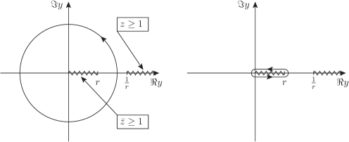
Figure 6: Position of the branch cuts in $z$ and $\bar{z}$ in the complex $y$-plane for $r<1$ (left). The contour along the unit circle in eq. (157) can be deformed and, consequently, identified with the integral of the $\bar{z}$-discontinuity (right), as written in eq. (158).

For $r<1$ there is a branch cut-free interval $(r,1/r)$ through which the contour along the unit circle passes, cf. the l.h.s. of figure 6. The contour can consequently be shrunk until it corresponds to integrating the $\bar{z}$-discontinuity of the wavefunction over $y$ from $0$ to $r$, cf. the r.h.s. of figure 6. We can now understand why it is necessary to work with the regularised integral $I_{\mathrm{reg}}$ of eq. (155) instead of the original $I$ of eq. (154): while the hard wavefunction $\Omega_{\mathrm{h}}(z,\bar{z})$ vanishes at 0 and $\infty$, its discontinuity, in general, does not. In other words, the contour deformation introduces spurious divergent terms and the cutoff introduced in eq. (155) regularises them. .

For $r>1$ the branch cuts of $z$ and $\bar{z}$ overlap. However, the discontinuity cancels identically in the interval $(1/r,r)$. Repeating the procedure, we again identify the contour integration with integrating the $\bar{z}$-discontinuity of $\Omega_{\mathrm{h}}(z,\bar{z})$ over $y$, this time, from $0$ to $1/r$.

In total, having modified the contour in (157) we find

$$I_{\mathrm{reg}} =\frac{1}{4\pi i}\left(\int_{\delta}^{1}\frac{\mathrm{d}r}{r}\int_{0}^{r}\frac{\mathrm{d}y}{y}\mathrm{disc_{\bar{z}}}[\Omega_{\mathrm{h}}(ry,r/y)]+\int_{1}^{1/\delta}\frac{\mathrm{d}r}{r}\int_{0}^{1/r}\frac{\mathrm{d}y}{y}\mathrm{disc_{\bar{z}}}[\Omega_{\mathrm{h}}(ry,r/y)]\right)$$

$$=\frac{1}{4\pi i}\left(\int_{\delta}^{1}\frac{\mathrm{d}r}{r}\int_{1}^{\infty}\frac{\mathrm{d}\bar{z}}{\bar{z}}\mathrm{disc_{\bar{z}}}[\Omega_{\mathrm{h}}(r^{2}/\bar{z},\bar{z})]+\int_{1}^{1/\delta}\frac{\mathrm{d}r}{r}\int_{0}^{1}\frac{\mathrm{d}z}{z}\mathrm{disc_{\bar{z}}}[\Omega_{\mathrm{h}}(z,r^{2}/z)]\right)$$

$$=\frac{1}{8\pi i}\left(\int_{1}^{\infty}\frac{\mathrm{d}\bar{z}}{\bar{z}}\int_{\delta^{2}/\bar{z}}^{1/\bar{z}}\frac{\mathrm{d}z}{z}\mathrm{disc_{\bar{z}}}[\Omega_{\mathrm{h}}(z,\bar{z})]+\int_{0}^{1}\frac{\mathrm{d}z}{z}\int_{1/z}^{1/(\delta^{2}z)}\frac{\mathrm{d}\bar{z}}{\bar{z}}\mathrm{disc_{\bar{z}}}[\Omega_{\mathrm{h}}(z,\bar{z})]\right)$$

$$=\frac{1}{8\pi i}\left(\int_{0}^{1}\frac{\mathrm{d}x}{x}\int_{\delta^{2}x}^{x}\frac{\mathrm{d}z}{z}\mathrm{disc_{\bar{z}}}[\Omega_{\mathrm{h}}(z,1/x)]+\int_{0}^{1}\frac{\mathrm{d}z}{z}\int_{\delta^{2}z}^{z}\frac{\mathrm{d}x}{x}\mathrm{disc_{\bar{z}}}[\Omega_{\mathrm{h}}(z,1/x)]\right)$$ (158)

where the two terms correspond respectively to $r<1$ and $r>1$. It is clear from the outset that they are equal: this corresponds to splitting (155) at $z\bar{z}=1$, which admits $(z,\bar{z})\leftrightarrow(1/z,1/\bar{z})$ symmetry. In the second line of (158) we reverted to the variable $\bar{z}=r/y$ in the first integral and $z=ry$ in the second; in the third we changed the order of integration before reverting to $z=r^{2}/\bar{z}$ in the first integral and $\bar{z}=r^{2}/z$ in the second; finally in the last line we defined $x=1/\bar{z}$ in the both integrals.

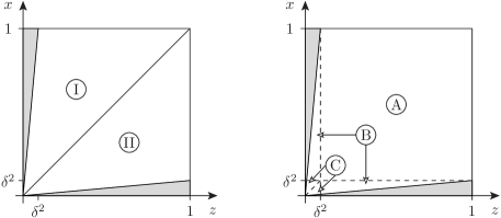
Figure 7: Illustration of the integrations in the $r<1$ (I) and $r>1$ (II) contribution to $I_{\mathrm{reg}}$ of eq. (157) (white triangles, l.h.s.). They can be viewed as the integral over a square (A) plus two wedges (B) minus two small triangles (C) (delimited by dashed lines, r.h.s.).

Let us now discuss the evaluation of the final expression in eq. (158), where the integration region of two terms is depicted as the white area in figure 7. In order to perform the integration it is useful to view the integrals (cf. the r.h.s. of figure 7) as the integral over a square

$$I_{A}(\delta)=\frac{1}{8\pi i}\int_{\delta^{2}}^{1}\frac{\mathrm{d}z}{z}\int_{\delta^{2}}^{1}\frac{\mathrm{d}x}{x}\mathrm{disc_{\bar{z}}}[\Omega_{\mathrm{h}}(z,1/x)]\,,$$ (159)

plus (the integrals over) two wedges

$$I_{B}(\delta)=\frac{1}{8\pi i}\left(\int_{0}^{1}\frac{\mathrm{d}x}{x}\int_{\delta^{2}x}^{\delta^{2}}\frac{\mathrm{d}z}{z}\mathrm{disc_{\bar{z}}}[\Omega_{\mathrm{h}}(z,1/x)]+\int_{0}^{1}\frac{\mathrm{d}z}{z}\int_{\delta^{2}z}^{\delta^{2}}\frac{\mathrm{d}x}{x}\mathrm{disc_{\bar{z}}}[\Omega_{\mathrm{h}}(z,1/x)]\right)\,,$$ (160)

minus two small triangles

$$I_{C}(\delta)=\frac{1}{8\pi i}\left(\int_{0}^{\delta^{2}}\frac{\mathrm{d}x}{x}\int_{\delta^{2}x}^{x}\frac{\mathrm{d}z}{z}\mathrm{disc_{\bar{z}}}[\Omega_{\mathrm{h}}(z,1/x)]+\int_{0}^{\delta^{2}}\frac{\mathrm{d}z}{z}\int_{\delta^{2}z}^{z}\frac{\mathrm{d}x}{x}\mathrm{disc_{\bar{z}}}[\Omega_{\mathrm{h}}(z,1/x)]\right)\,,$$ (161)

where both $z$ and $x$ are small. Next we would like to evaluate each of these contributions, distinguishing between finite, $\delta$-independent terms, and logarithmically divergent cut-off dependent terms.

The discontinuity w.r.t. $\bar{z}$ of $\Omega_{\mathrm{h}}(z,1/x)$ evaluates to hpls of $z$ and $x$. $I_{A}(\delta)$ of eq. (159) thus immediately evaluates to hpls at 1, giving rise to mzvs, and at $\delta^{2}$; the latter contain logarithmically divergent terms in $\delta$. The first (second) integral in the expression of $I_{B}(\delta)$ in (160) is calculated close to $z=0$ ($x=0$), cf. figure 7. One can therefore expand the discontinuity function in the integrand and discard terms suppressed by powers of $z$ ($x$) keeping only powers of $\log z$ ($\log x$). The inner integrals then yield powers of $\log\delta^{2}$, $\log\delta^{2}x=\log x+\log\delta^{2}$ and $\log\delta^{2}z=\log z+\log\delta^{2}$, respectively. The outer integrals thereupon generate mzvs from their upper limits; in addition it contains logarithmically divergent terms in $\delta$. Contributions from the lower integration limits are dropped according to the (standard) regularisation of hpls:

$$\lim_{z\to 0}\log z=0.$$ (162)

A similar analysis of $I_{C}(\delta)$ in eq. (161) reveals that only powers of $\log\delta^{2}$ are generated by the integrations over the two small triangles in figure 7.

Since the original integral $I$ of eq. (154) is finite and $I_{\mathrm{reg}}\to I$ for $\delta\to 0$ all terms proportional to $\log\delta^{2}$ have to cancel between the three contributions $I_{A}(\delta)$, $I_{B}(\delta)$ and $I_{C}(\delta)$. This enables us to derive a simplified integral in which the logarithmically divergent terms are absent altogether whilst giving the same finite terms:

$$I_{\mathrm{reg}}=\frac{1}{8\pi i}\int_{0}^{1}\frac{\mathrm{d}z}{z}\int_{0}^{1}\frac{\mathrm{d}x}{x}\mathrm{disc_{\bar{z}}}[\Omega_{\mathrm{h}}(z,1/x)]\\ +\frac{1}{8\pi i}\left(-\int_{0}^{1}\frac{\mathrm{d}x}{x}\int_{0}^{x}\frac{\mathrm{d}z}{z}\mathrm{disc_{\bar{z}=1}}[\Omega_{\mathrm{h}}(z,1/x)]\big{|}_{z\ll 1}\right.\\ \left.-\int_{0}^{1}\frac{\mathrm{d}z}{z}\int_{0}^{z}\frac{\mathrm{d}x}{x}\mathrm{disc_{\bar{z}=1}}[\Omega_{\mathrm{h}}(z,1/x)]\big{|}_{x\ll 1}\right)\,,$$ (163)

where all integrals are regulated according to eq. (162) and $\mathrm{disc_{\bar{z}=1}}[\Omega_{\mathrm{h}}(z,1/x)]\big{|}_{z\ll 1}$ and $\mathrm{disc_{\bar{z}=1}}[\Omega_{\mathrm{h}}(z,1/x)]\big{|}_{x\ll 1}$ refer to the aforementioned expansion of the integrand around small $z$ and $x$, respectively. The first integral in eq. (163) reproduces all finite, cut-off independent terms in $I_{A}(\delta)$ of (159), while the second and third ones reproduce, respectively, the finite terms in the two integral in $I_{B}(\delta)$ in (160); finally, given that no cut-off independent terms are produce by $I_{C}(\delta)$, it has no trace in (163).

The above calculation is biased towards the discontinuity with respect to $\bar{z}$ which is purely a matter of choice. A similar calculation can be performed to get an answer in terms of the discontinuity with respect to $z$ or a mixed expression that features both discontinuities.

This integration method was further checked as follows. Given a wavefunction (or svhpl) we expand around $z=\bar{z}=0$ and change variables to the polar coordinates introduced above in eq. (157). The result is a sum of terms of the form $r^{a}y^{b}\log^{c}(r^{2})$ with rational constant coefficients and $a,c\geq 0$ and $b$ are integer powers. Integrating the azimuth over $[0,\,2\pi]$ then removes all terms that explicitely depend on $y$, i.e. that have $b\neq 0$. Next, we determine the rational coefficients in terms of harmonic numbers. This enables us to perform the sum ad infinitum after we integrate term-by-term with respect to $r$.

5.2 Method II: final integration as an action of the Hamiltonian

The previous method, albeit straightforward on paper, is computationally demanding at high loop orders as it requires extensive use of analytic continuations of hpls to calculate discontinuities. It turns out there is an easier way to perform the final integration, which lets us make use of our knowledge about the action of the Hamiltonian, established upon computing the wavefunction in section 4.

Consider the action of $\hat{H}_{\mathrm{2d,i}}$ (91a) on the wavefunction $\Omega_{\mathrm{h}}(1-z,1-\bar{z})$

$$\hat{H}_{\mathrm{2d,i}}\Omega_{\mathrm{h}}(1-z,1-\bar{z})=\frac{1}{4\pi}\int\mathrm{d}^{2}wK(w,\bar{w},z,\bar{z})\Big{[}\Omega_{\mathrm{h}}(1-w,1-\bar{w})-\Omega_{\mathrm{h}}(1-z,1-\bar{z})\Big{]}$$ (164)

and set $z=\bar{z}=1$ under the integral. Using $\Omega_{\mathrm{h}}(0,0)=0$ one gets on the right-hand side:

$$\lim_{z,\bar{z}\to 1}K(w,\bar{w},z,\bar{z})\Big{[}\Omega_{\mathrm{h}}(1-w,1-\bar{w})-\Omega_{\mathrm{h}}(1-z,1-\bar{z})\Big{]}=K(w,\bar{w},1,1)\Omega_{\mathrm{h}}(1-w,1-\bar{w})$$ (165)

with the kernel

$$K(w,\bar{w},1,1)=\frac{1}{w\bar{w}(1-w)(1-\bar{w})}+\frac{1}{(1-w)(1-\bar{w})}-\frac{1}{w\bar{w}},$$ (166)

cf. eq. (85). It thus follows that (164), taken in the limit $z,\bar{z}\to 1$, yields:

$$\begin{split}&\hat{H}_{\mathrm{2d,i}}\Omega_{\mathrm{h}}(1-z,1-\bar{z})\big{|}_{z,\bar{z}\to 1}=\\ &\hskip 20.0pt=\,\frac{1}{4\pi}\int\mathrm{d}^{2}w\left[\frac{\Omega_{\mathrm{h}}(1-w,1-\bar{w})}{w\bar{w}(1-w)(1-\bar{w})}+\frac{\Omega_{\mathrm{h}}(1-w,1-\bar{w})}{(1-w)(1-\bar{w})}-\frac{\Omega_{\mathrm{h}}(1-w,1-\bar{w})}{w\bar{w}}\right]\\ &\hskip 20.0pt=\,\frac{1}{4\pi}\int\frac{\mathrm{d}^{2}w}{w\bar{w}}\left[\Omega_{\mathrm{h}}\left(\frac{1}{1-w},\frac{1}{1-w}\right)+\Omega_{\mathrm{h}}(w,\bar{w})-\Omega_{\mathrm{h}}(1-w,1-\bar{w})\right]\,,\end{split}$$ (167)

where in the second line we changed the integration variables in the first two terms – in the first using $w\rightarrow w/(w-1)$, and in the second using $w\rightarrow 1-w$, and then factored out a common denominator. Given that the wavefunction is symmetric under inversion, $\Omega_{\mathrm{h}}(1/w,1/\bar{w})=\Omega_{\mathrm{h}}(w,\bar{w})$, the first and third terms in the last equation cancel and we find

$$\hat{H}_{\mathrm{2d,i}}\Omega_{\mathrm{h}}(1-z,1-\bar{z})\big{|}_{z,\bar{z}\to 1}=\frac{1}{4\pi}\int\frac{\mathrm{d}^{2}w}{w\bar{w}}\Omega_{\mathrm{h}}(w,\bar{w})=I\,,$$ (168)

which can be readily identified with the integral in eq. (154) which we are interested to compute.

We thus conclude that the integral in eq. (153), representing the hard wavefunction contribution to the reduced amplitude, integrated in exactly two dimensions, may be calculated with the methods we developed for the computation of the two-dimensional wavefunction itself, described in section 4.1. In practice one rewrites the wavefunction $\Omega_{\mathrm{h}}(1-z,1-\bar{z})$ in terms of svhpls of $z$ and $\bar{z}$, then applies the Hamiltonian by solving the corresponding differential equations, and finally evaluates the resulting expression at $z,\bar{z}=1$. The last step produces the anticipated mzvs.

Method I, described in section 5.1, and method II outlined here show perfect agreement when applied to the wavefunction. However, we emphasise that while former may be applied on individual svhpls, the latter can only be applied to expressions which are symmetric under inversion of their arguments, cf. eqs. (167) and (168).

5.3 Results for the reduced amplitude

With the methods described in the previous sections it is straightforward to integrate the two-dimensional wavefunction and thereby compute the hard contribution to the amplitude, namely the finite terms not captured by the soft limit.

Before presenting our results let us recall the number-theoretic observations we made about the amplitude at the end of section 2. There, we claimed that the $\ell$-loop amplitude (divided by $B_{0}^{\ell}$, (8)) has two important number-theoretic properties: all of its terms have weight $\ell$ and there are no terms proportional to $\zeta_{2}$. We proved this statement for contributions from the soft limit in section 3, see below eq. (64). We now show that it holds also for the hard contributions.

We begin by noting that the integrand in (154) is expressed as a pure function of uniform weight, written as sums of products of HPLs. We note that both methods for the last integral, in sections 5.1 and 5.2, increase the weight of the functions they act on by one, before evaluating the result at $z=\bar{z}=1$. In method I the action of the discontinuity first lowers the weight of its argument by one; this is then compensated by two consecutive integrations of a $d\log$ form, each raising the weight by one. Method II, in turn, applies the Hamiltonian $\hat{H}_{\mathrm{2d,i}}$ on the wavefunction after a variable transformation $z\to 1-z$. Changing the variables of an svhpl does obviously not change its weight and the action of the Hamiltonian corresponds to integrating a first-order differential equation, which raises the weight of the operand by one.

svhpls at $z=\bar{z}=1$ evaluate to multiple zeta values (mzvs) of the same weight, as discussed following eqs. (129a)–(129d). We remind the reader that the $(\ell-1)$-loop wavefunction consists of weight-$(\ell-1)$ svhpls and weight-$(\ell-1)$ products of svhpls and zeta numbers and conclude that the hard contributions to the $\ell$-loop amplitude therefore have uniform weight $\ell$. The absence of $\zeta_{2}$ in the hard component $\hat{\mathcal{M}}_{{\rm NLL,h}}^{(+,\ell)}$ is readily explained by the fact that svhpls can, by construction, only ever evaluate to odd zeta numbers, for any argument.

We start the discussion of the results by presenting the contributions that originate in the hard region. They are the immediate result of the previous sections and, through eight loops, read

$$\hat{\mathcal{M}}_{{\rm NLL,h}}^{(+,1)} =0,$$ (169a)

$$\hat{\mathcal{M}}_{{\rm NLL,h}}^{(+,2)} =0,$$ (169b)

$$\hat{\mathcal{M}}_{{\rm NLL,h}}^{(+,3)} =\frac{i\pi}{3!}\bigg{\{}\frac{3\zeta_{3}}{4}C_{1}C_{2}\bigg{\}}\mathbf{T}_{s-u}^{2}\mathcal{M}^{\mathrm{(tree)}},$$ (169c)

$$\hat{\mathcal{M}}_{{\rm NLL,h}}^{(+,4)} =0,$$ (169d)

$$\hat{\mathcal{M}}_{{\rm NLL,h}}^{(+,5)} =\frac{i\pi}{5!}\bigg{\{}-\frac{5\zeta_{5}}{2}C_{1}^{2}C_{2}^{2}+\,\frac{45\zeta_{5}}{2}C_{1}C_{2}^{3}\bigg{\}}\mathbf{T}_{s-u}^{2}\mathcal{M}^{\mathrm{(tree)}},$$ (169e)

$$\hat{\mathcal{M}}_{{\rm NLL,h}}^{(+,6)} =\frac{i\pi}{6!}\bigg{\{}\frac{39\zeta_{3}^{2}}{16}C_{1}^{3}C_{2}^{2}-\frac{45\zeta_{3}^{2}}{2}C_{1}^{2}C_{2}^{3}+\,\frac{225\zeta_{3}^{2}}{2}C_{1}C_{2}^{4}\bigg{\}}\mathbf{T}_{s-u}^{2}\mathcal{M}^{\mathrm{(tree)}},$$ (169f)

$$\hat{\mathcal{M}}_{{\rm NLL,h}}^{(+,7)} =\frac{i\pi}{7!}\bigg{\{}-\frac{2135\zeta_{7}}{256}C_{1}^{4}C_{2}^{2}+\frac{30135\zeta_{7}}{256}C_{1}^{3}C_{2}^{3}-\,\frac{20111\zeta_{7}}{32}C_{1}^{2}C_{2}^{4}$$

$$\hskip 113.81102pt+\frac{6111\zeta_{7}}{4}C_{1}C_{2}^{5}\bigg{\}}\mathbf{T}_{s-u}^{2}\mathcal{M}^{\mathrm{(tree)}},$$ (169g)

$$\hat{\mathcal{M}}_{{\rm NLL,h}}^{(+,8)} =\frac{i\pi}{8!}\bigg{\{}\frac{611\zeta_{3}\zeta_{5}}{32}C_{1}^{5}C_{2}^{2}-\frac{643\zeta_{3}\zeta_{5}}{2}C_{1}^{4}C_{2}^{3}+\frac{8597\zeta_{3}\zeta_{5}}{4}C_{1}^{3}C_{2}^{4}$$

$$\hskip 56.9055pt-7086\zeta_{3}\zeta_{5}\,C_{1}^{2}C_{2}^{5}+\,13230\zeta_{3}\zeta_{5}\,C_{1}C_{2}^{6}\bigg{\}}\mathbf{T}_{s-u}^{2}\mathcal{M}^{\mathrm{(tree)}},$$ (169h)

where we again used the shorthand notation for the colour factors, $C_{1}=2C_{A}-\mathbf{T}_{t}^{2}$ and $C_{2}=C_{A}-\mathbf{T}_{t}^{2}$. One may observe the aforementioned homogeneous weight property and absence of even zeta numbers. In fact, considering the first eight loop orders, one may get the false impression that each order contains just a single (product) of zeta numbers and that they are all single (ordinary) zeta numbers. Both these features are artefacts of looking at low weights, and a much richer structure will be revealed at higher loop orders, as we discuss shortly.

Given the identity in eq. (76b), i.e. $\mathcal{H}^{(+)}_{\rm NLL,h}={\cal\hat{M}}^{(+)}_{\rm NLL,h}$, the result of (169) is sufficient to compute the full infrared-renormalized amplitude $\mathcal{H}^{(+)}_{\rm NLL}$ by combining it with the soft contribution $\mathcal{H}^{(+)}_{\rm NLL,s}$ of eqs. (79) and (80a). This will be done in the section 5.4 below. Before doing this let us combine the hard and soft components for the reduced amplitude itself, and comment further on some number-theoretic properties, as promised.

According to eqs. (50) and (51), the expressions for the full reduced amplitude through ${\cal O}(\epsilon^{0})$ can be easily obtained order-by-order summing the results for the soft amplitude provided in eqs. (64a)-(64) and those for the hard amplitude in eqs. (169a)–(169h) above, where the former accounts for all infrared singularities plus some finite terms, and the latter for the remaining finite contributions. We obtain

$$\hat{\mathcal{M}}_{\rm NLL}^{(1)} =i\pi B_{0}\bigg{\{}\frac{1}{2\epsilon}\bigg{\}}\mathbf{T}_{s-u}^{2}\mathcal{M}^{\mathrm{(tree)}},$$ (170a)

$$\hat{\mathcal{M}}_{\rm NLL}^{(2)} =i\pi\frac{B_{0}^{2}}{2}\bigg{\{}\frac{C_{2}}{4\epsilon^{2}}\bigg{\}}\mathbf{T}_{s-u}^{2}\mathcal{M}^{\mathrm{(tree)}},$$ (170b)

$$\hat{\mathcal{M}}_{\rm NLL}^{(3)} =i\pi\frac{B_{0}^{3}}{3!}\bigg{\{}C_{2}^{2}\left(\frac{1}{8\epsilon^{3}}-\frac{11\zeta_{3}}{4}\right)\bigg{\}}\mathbf{T}_{s-u}^{2}\mathcal{M}^{\mathrm{(tree)}},$$ (170c)

$$\hat{\mathcal{M}}_{\rm NLL}^{(4)} =i\pi\frac{B_{0}^{4}}{4!}\bigg{\{}C_{1}C_{2}^{2}\left(-\frac{\zeta_{3}}{8\epsilon}-\frac{3\zeta_{4}}{16}\right)+C_{2}^{3}\left(\frac{1}{16\epsilon^{4}}+\frac{\zeta_{3}}{8\epsilon}+\frac{3\zeta_{4}}{16}\right)\bigg{\}}\mathbf{T}_{s-u}^{2}\mathcal{M}^{\mathrm{(tree)}},$$ (170d)

$$\hat{\mathcal{M}}_{\rm NLL}^{(5)} =i\pi\frac{B_{0}^{5}}{5!}\bigg{\{}C_{1}^{2}C_{2}^{2}\left(-\frac{5\zeta_{5}}{2}\right)+C_{1}C_{2}^{3}\left(-\frac{\zeta_{3}}{16\epsilon^{2}}-\frac{3\zeta_{4}}{32\epsilon}+\frac{333\zeta_{5}}{16}\right)$$

$$\hskip 28.45274pt+\,C_{2}^{4}\left(\frac{1}{32\epsilon^{5}}+\frac{\zeta_{3}}{16\epsilon^{2}}+\frac{3\zeta_{4}}{32\epsilon}-\frac{717\zeta_{5}}{16}\right)\bigg{\}}\mathbf{T}_{s-u}^{2}\mathcal{M}^{\mathrm{(tree)}},$$ (170e)

$$\hat{\mathcal{M}}_{\rm NLL}^{(6)} =i\pi\frac{B_{0}^{6}}{6!}\bigg{\{}C_{1}^{3}C_{2}^{2}\bigg{(}\frac{39\zeta_{3}^{2}}{16}\bigg{)}+C_{1}^{2}C_{2}^{3}\bigg{(}-\frac{399\zeta_{3}^{2}}{16}\bigg{)}$$

$$\hskip 28.45274pt+\,C_{1}C_{2}^{4}\bigg{(}-\frac{\zeta_{3}}{32\epsilon^{3}}-\frac{3\zeta_{4}}{64\epsilon^{2}}-\frac{3\zeta_{5}}{32\epsilon}+\frac{2637\zeta_{3}^{2}}{32}+\frac{5\zeta_{6}}{32}\bigg{)}$$

$$\hskip 28.45274pt+\,C_{2}^{5}\bigg{(}\frac{1}{64\epsilon^{6}}+\frac{\zeta_{3}}{32\epsilon^{3}}+\frac{3\zeta_{4}}{64\epsilon^{2}}+\frac{3\zeta_{5}}{32\epsilon}-\frac{2879\zeta_{3}^{2}}{32}+\frac{5\zeta_{6}}{32}\bigg{)}\bigg{\}}\mathbf{T}_{s-u}^{2}\mathcal{M}^{\mathrm{(tree)}},$$ (170f)

$$\hat{\mathcal{M}}_{\rm NLL}^{(7)} =i\pi\frac{B_{0}^{6}}{6!}\bigg{\{}C_{1}^{4}C_{2}^{2}\bigg{(}\frac{2135\zeta_{7}}{256}\bigg{)}C_{1}^{3}C_{2}^{3}\bigg{(}\frac{30135\zeta_{7}}{256}\bigg{)}+C_{1}^{2}C_{2}^{4}\bigg{(}\frac{\zeta_{3}^{2}}{32\epsilon}+\frac{3\zeta_{3}\zeta_{4}}{32}-\,\frac{20111\zeta_{7}}{32}\bigg{)}$$

$$\hskip 28.45274pt+C_{1}C_{2}^{5}\bigg{(}-\frac{\zeta_{3}}{64\epsilon^{4}}-\frac{3\zeta_{4}}{128\epsilon^{3}}-\frac{3\zeta_{5}}{64\epsilon^{2}}-\frac{3\zeta_{3}^{2}}{64\epsilon}-\frac{5\zeta_{6}}{64\epsilon}-\frac{9\zeta_{3}\zeta_{4}}{64}+\,\frac{97047\zeta_{7}}{64}\bigg{)}$$

$$\hskip 28.45274pt+C_{2}^{6}\bigg{(}\frac{1}{128\epsilon^{7}}+\frac{\zeta_{3}}{64\epsilon^{4}}+\frac{3\zeta_{4}}{128\epsilon^{3}}+\frac{3\zeta_{5}}{64\epsilon^{2}}+\frac{\zeta_{3}^{2}}{64\epsilon}+\frac{5\zeta_{6}}{64\epsilon}$$

$$\hskip 28.45274pt+\,\frac{3\zeta_{3}\zeta_{4}}{64}-\frac{90711\zeta_{7}}{64}\bigg{)}\bigg{\}}\mathbf{T}_{s-u}^{2}\mathcal{M}^{\mathrm{(tree)}},$$ (170g)

$$\hat{\mathcal{M}}_{\rm NLL}^{(8)} =i\pi\frac{B_{0}^{8}}{8!}\bigg{\{}C_{1}^{5}C_{2}^{2}\bigg{(}\frac{611\zeta_{3}\zeta_{5}}{32}\bigg{)}+C_{1}^{4}C_{2}^{3}\bigg{(}-\frac{643\zeta_{3}\zeta_{5}}{2}\bigg{)}+C_{1}^{3}C_{2}^{4}\bigg{(}\frac{8597\zeta_{3}\zeta_{5}}{4}\bigg{)}$$

$$\hskip 28.45274pt+\,C_{1}^{2}C_{2}^{5}\bigg{(}\frac{\zeta_{3}^{2}}{64\epsilon^{2}}+\frac{3\zeta_{3}\zeta_{4}}{64\epsilon}-\frac{228093\zeta_{3}\zeta_{5}}{32}+\frac{21\zeta_{8}}{512}\bigg{)}+C_{1}C_{2}^{6}\bigg{(}-\frac{\zeta_{3}}{128\epsilon^{5}}$$

$$\hskip 28.45274pt-\,\frac{3\zeta_{4}}{256\epsilon^{4}}-\frac{3\zeta_{5}}{128\epsilon^{3}}-\frac{3\zeta_{3}^{2}}{128\epsilon^{2}}-\frac{5\zeta_{6}}{128\epsilon^{2}}-\frac{9\zeta_{3}\zeta_{4}}{128\epsilon}-\frac{9\zeta_{7}}{128\epsilon}+\frac{749943\zeta_{3}\zeta_{5}}{64}$$

$$\hskip 28.45274pt-\,\frac{189\zeta_{8}}{1024}\bigg{)}+C_{2}^{7}\bigg{(}\frac{1}{256\epsilon^{8}}+\frac{\zeta_{3}}{128\epsilon^{5}}+\frac{3\zeta_{4}}{256\epsilon^{4}}+\frac{3\zeta_{5}}{128\epsilon^{3}}+\frac{\zeta_{3}^{2}}{128\epsilon^{2}}+\frac{5\zeta_{6}}{128\epsilon^{2}}$$

$$\hskip 28.45274pt+\frac{3\zeta_{3}\zeta_{4}}{128\epsilon}+\frac{9\zeta_{7}}{128\epsilon}-\frac{483837\zeta_{3}\zeta_{5}}{64}+\frac{147\zeta_{8}}{1024}\bigg{)}\bigg{\}}\mathbf{T}_{s-u}^{2}\mathcal{M}^{\mathrm{(tree)}}\,,$$ (170h)

These result reproduce the one- to four-loop results of ref. Caron-Huot:2013fea and of our numerically-determined five-loop result in eq. (37). In the ancillary file NLL-reduced-amplitude.txt we provide the result for the soft, the hard and the full reduced amplitude up to 13 loops. Furthermore, the amplitude can now be calculated to any number of loops with the methods presented in sections 3, 4 and 5.

Similarly to the wavefunction at twelve loops (and above), the hard contributions to the amplitude (and thus the full amplitude itself) cannot be expressed in terms of ordinary zeta numbers beyond a certain loop order. In fact, most of what we discussed in the context of the wavefunction below eqs. (129a)–(129d) applies to the amplitude as well: Either of the two methods presented in section 5.1 and 5.2 requires us to evaluate svhpls at $z=\bar{z}=1$ and we hence expect the presence of (single-valued) mzvs starting from weight eleven. Indeed, the eleven-loop amplitude features a term proportional to $g_{5,3,3}$, defined in eq. (130):

$$\hat{\mathcal{M}}_{\mathrm{NLL}}^{(+,{11})}\supset\frac{1}{102400}\bigg{(}-\frac{149}{6720}C_{1}^{8}C_{2}^{2}+\frac{26209}{60480}C_{1}^{7}C_{2}^{3}-\frac{14813}{4320}C_{1}^{6}C_{2}^{4}+\frac{210383}{15120}C_{1}^{5}C_{2}^{5}\\ -\frac{7549}{252}C_{1}^{4}C_{2}^{6}+\frac{39257}{1260}C_{1}^{3}C_{2}^{7}-11C_{1}^{2}C_{2}^{8}\bigg{)}\times g_{5,3,3}.$$ (171)

Of course this term is entirely due to the hard component of the amplitude, as the soft one consists exclusively of ordinary zeta values (non-single-valued ones), as discussed in section 3. At twelve loops the reduced amplitude is again comprised of ordinary zeta numbers $\zeta_{n}$, as there are no weight 12 single-valued MZVs. Such numbers appear then again in the thirteen loop amplitude:

$$\hat{\mathcal{M}}_{\mathrm{NLL}}^{(+,{13})}\supset\frac{1}{2207744000}\bigg{(}\frac{5367943}{497664}C_{1}^{10}C_{2}^{2}-\frac{32668315}{124416}C_{1}^{9}C_{2}^{3}+\frac{6876365071}{2488320}C_{1}^{8}C_{2}^{4}\\ -\frac{10213439791}{622080}C_{1}^{7}C_{2}^{5}+\frac{37444840199}{622080}C_{1}^{6}C_{2}^{6}-\frac{10827306157}{77760}C_{1}^{5}C_{2}^{7}\\ +\frac{3841520891}{19440}C_{1}^{4}C_{2}^{8}-\frac{503783639}{3240}C_{1}^{3}C_{2}^{9}+50459C_{1}^{2}C_{2}^{10}\bigg{)}\times g_{5,5,3},$$ (172)

and

$$\hat{\mathcal{M}}_{\mathrm{NLL}}^{(+,{13})}\supset\frac{1}{2649292800}\bigg{(}-\frac{1819475}{82944}C_{1}^{10}C_{2}^{2}+\frac{5621717}{10368}C_{1}^{9}C_{2}^{3}-\frac{961202489}{165888}C_{1}^{8}C_{2}^{4}\\ +\frac{482408111}{13824}C_{1}^{7}C_{2}^{5}-\frac{5356152533}{41472}C_{1}^{6}C_{2}^{6}+\frac{1551101681}{5184}C_{1}^{5}C_{2}^{7}\\ -\frac{543921901}{1296}C_{1}^{4}C_{2}^{8}+\frac{69045265}{216}C_{1}^{3}C_{2}^{9}-96967C_{1}^{2}C_{2}^{10}\bigg{)}\times g_{7,3,3},$$ (173)

where the single-values zeta numbers $g_{5,5,3}$ and $g_{7,3,3}$ have been defined in eqs. (132) and (133).

The fact that the MZV terms in eqs. (171), (172) and (173) appear in the eleven- and thirteen-loop amplitude already excludes that there could be a simple all-order formula in terms of gamma functions for the reduced amplitude. This stands in sharp contrast to the contributions associated with the soft limit, both singular and finite, which can be resummed to all orders by means of gamma functions, as we have seen in section 3.

5.4 The infrared-renormalized amplitude

We conclude this section by discussing the perhaps most physically relevant infrared-renormalized amplitude (or hard function), which according to eq. (75), is obtained by summing the soft component, given to all orders by the closed expression in eq. (79), and the hard component, which according to eq. (76b), coincides with the hard component of the reduced amplitude, ${\cal\hat{M}}^{(+)}_{\rm NLL,h}$. The latter can be determined to any loop order by following the methods discussed in sections 5.1 and 5.2, however a closed-form expression cannot be obtained as in case of the soft part of the infrared-renormalized amplitude. Thus, in practice we limit ourselves to determine this amplitude to 13 loops, and the result is provided in the ancillary file NLL-IR-renormalised-amplitude.txt. Here we provide a sample of the result (with ${\cal H}$ defined in eq. (38) and loop-expanded following eq. (21)), up to eight loops:

$${\cal H}_{\rm NLL}^{(1)} =0,$$ (174a)

$${\cal H}_{\rm NLL}^{(2)} =0,$$ (174b)

$${\cal H}_{\rm NLL}^{(3)} =\frac{i\pi}{3!}\bigg{\{}-C_{2}^{2}\frac{11\zeta_{3}}{4}\bigg{\}}\mathbf{T}_{s-u}^{2}\mathcal{M}^{\mathrm{(tree)}},$$ (174c)

$${\cal H}_{\rm NLL}^{(4)} =\frac{i\pi}{4!}\bigg{\{}-C_{A}C_{2}^{2}\frac{3\zeta_{4}}{16}\bigg{\}}\mathbf{T}_{s-u}^{2}\mathcal{M}^{\mathrm{(tree)}},$$ (174d)

$${\cal H}_{\rm NLL}^{(5)} =\frac{i\pi}{5!}\bigg{\{}-C_{A}^{2}C_{2}^{2}\frac{5\zeta_{5}}{2}+C_{A}C_{2}^{3}\frac{253\zeta_{5}}{16}-C_{2}^{4}\frac{53\zeta_{5}}{2}\bigg{\}}\mathbf{T}_{s-u}^{2}\mathcal{M}^{\mathrm{(tree)}},$$ (174e)

$${\cal H}_{\rm NLL}^{(6)} =\frac{i\pi}{6!}\bigg{\{}C_{A}^{3}C_{2}^{2}\frac{39\zeta_{3}^{2}}{16}-C_{A}^{2}C_{2}^{3}\frac{141\zeta_{3}^{2}}{8}+C_{A}C_{2}^{4}\bigg{(}\frac{1275\zeta_{3}^{2}}{32}-\,\frac{5\zeta_{6}}{32}\bigg{)}$$

$$\hskip 56.9055pt-C_{2}^{5}\frac{481\zeta_{3}^{2}}{16}\bigg{\}}\mathbf{T}_{s-u}^{2}\mathcal{M}^{\mathrm{(tree)}},$$ (174f)

$${\cal H}_{\rm NLL}^{(7)} =\frac{i\pi}{7!}\bigg{\{}-C_{A}^{4}C_{2}^{2}\frac{2135\zeta_{7}}{256}+C_{A}^{3}C_{2}^{3}\frac{21595\zeta_{7}}{256}+C_{A}^{2}C_{2}^{4}\bigg{(}\frac{3\zeta_{3}\zeta_{4}}{32}-\frac{83293\zeta_{7}}{256}\bigg{)}$$

$$\hskip 56.9055pt+\,C_{A}C_{2}^{5}\bigg{(}\frac{3\zeta_{3}\zeta_{4}}{64}+\frac{148277\zeta_{7}}{256}\bigg{)}-C_{2}^{6}\frac{13443\zeta_{7}}{32}\bigg{\}}\mathbf{T}_{s-u}^{2}\mathcal{M}^{\mathrm{(tree)}},$$ (174g)

$${\cal H}_{\rm NLL}^{(8)} =\frac{i\pi}{8!}\bigg{\{}C_{A}^{5}C_{2}^{2}\frac{611\zeta_{3}\zeta_{5}}{32}-C_{A}^{4}C_{2}^{3}\frac{7233\zeta_{3}\zeta_{5}}{32}+C_{A}^{3}C_{2}^{4}\frac{16867\zeta_{3}\zeta_{5}}{16}+C_{A}^{2}C_{2}^{5}\bigg{(}-\frac{77383\zeta_{3}\zeta_{5}}{32}$$

$$\hskip 28.45274pt+\,\frac{21\zeta_{8}}{512}\bigg{)}+C_{A}C_{2}^{6}\bigg{(}\frac{174033\zeta_{3}\zeta_{5}}{64}-\frac{105\zeta_{8}}{1024}\bigg{)}-C_{2}^{7}\frac{35941\zeta_{3}\zeta_{5}}{32}\bigg{\}}\mathbf{T}_{s-u}^{2}\mathcal{M}^{\mathrm{(tree)}}\,.$$ (174h)

Given that $\mathcal{H}^{(+)}_{\rm NLL,h}={\cal\hat{M}}^{(+)}_{\rm NLL,h}$, the same number-theory properties discussed at the end of section 5.3 apply to the infrared-renormalized amplitude as well. In particular, resummation in terms of gamma functions is excluded.

6 Numerical analysis and convergence properties

The calculation developed in sections 3, 4 and 5 has allowed us to determine symmetries and general features of the wavefunction and the amplitude, as well as their exact analytic structure to fourteen and thirteen orders in perturbation theory respectively. We are now interested to perform a numerical analysis, and focus on features which are not directly evident from the analytic expressions, such as the qualitative behaviour of the wavefunction, the relative size of the soft and hard contributions to the wavefunction, and the convergence properties of the infrared-renormalized amplitude as an expansion in $x\equiv L\,\alpha_{s}/\pi$.

6.1 Wavefunction

Let us begin by analysing the wavefunction. Given its finiteness, we consider here the leading term in the $\epsilon$ expansion, i.e. the two-dimensional soft, hard and full wavefunctions, defined respectively in eqs. (151), (49) and (89).

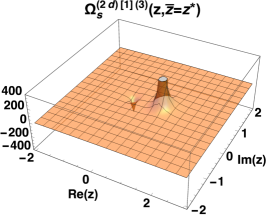
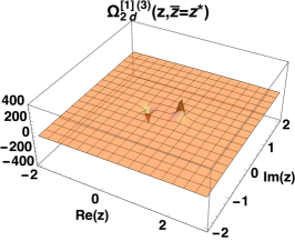
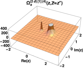
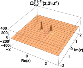
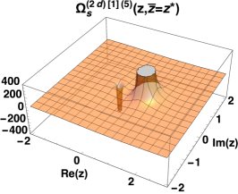
Figure 8: Soft, hard and full wavefunction in the complex plane ${\rm Re}(z)$, ${\rm Im}(z)$. Here we plot the singlet component of the wavefunction. The soft and the full wavefunction exhibit singularities at $z=0$ and $z=\infty$, due to the $z\leftrightarrow 1/z$ symmetry, (the latter is not visible in the plots). In addition, there is a singularity at $z=1$, which appears also in the hard part of the wavefunction. Notice that the singularities at $z=1$ partly cancel between the soft and hard wavefunctions, such that the full wavefunction exhibits a peak near $z=1$ which is markedly smaller relative to the two separate contributions.

As an example, in figures 8 and 9 we plot the coefficients $\Omega_{\rm s}^{(\rm 2d)(\ell)}$, $\Omega_{\rm h}^{(\rm 2d)(\ell)}$, $\Omega_{\rm 2d}^{(\ell)}$, at third, fourth and fifth order in perturbation theory. In these plots we fix $N_{c}=3$ and consider specific colour representations, namely the singlet and the 27 representation, such that the Casimir operator in the $t$-channel evaluates to

$$\begin{array}[]{ll}\text{singlet}:&{\mathbf{T}}_{t}^{2}\,{\cal M}^{[1]}=0,\\ \text{27 representation}:&{\mathbf{T}}_{t}^{2}\,{\cal M}^{[27]}=2(N_{c}+1)\,{\cal M}^{[27]}=8\,{\cal M}^{[27]}.\end{array}$$ (177)

We plot the wavefunction in the complex $z$ plane, for $\bar{z}=z^{*}$. We observe that the soft and full wavefunctions exhibit peaks at $z=0$; these are associated with the soft limit. Of course, by the $z\leftrightarrow 1/z$ symmetry discussed in sections 4.1 and 4.3, there is an identical singularity at $z=\infty$ (which is not visible in the patch of the complex plane shown in the plot). In the way we separated between the soft and hard components, the two-dimensional hard wavefunction is strictly zero in these soft limits (see the discussion following eq. (155)).

All components of the wavefunction have singularities at $z=1$. The $z=1$ singularity represents rather different physics, where both Reggeons are hard, namely $k^{2},(p-k)^{2}\gg p^{2}$. It is interesting to note that the singularity at $z=1$ is always of opposite sign between the soft and hard wavefunction, such that these contributions cancel to a large extent in the full wavefunction. This observation allows us to conclude already that the soft approximation, although convenient for calculation purposes, does not provide a good numerical approximation for the full wavefunction away from the soft limit.

Focusing now on the full wavefunction, the singular behaviour near $z=0$ and $z=1$ at $\ell$ loop order can be described respectively by the leading logarithms in the two limits, $\sim c_{\ell}\log^{\ell}(z\bar{z})$ and $\sim c^{\prime}_{\ell}\log^{\ell}\big{[}1/(1-z)^{2}(1-\bar{z})^{2}\big{]}$, where both the magnitude and the sign of the coefficients $c_{\ell}$ and $c_{\ell}^{\prime}$ depends on the colour representation considered. Concerning the limit $z=0$, the asymptotic behaviour is entirely determined by the soft wavefunction, given that $\Omega_{\rm h}^{\rm 2d}(0,0)=0$. We obtain the coefficients $c_{\ell}$ expanding the soft function in eq. (152) (compare eqs. (61) and (3.3)). Taking into account eq. (18), we find

$$\Omega^{({\ell})}(z,\bar{z})|_{z\to 0}\simeq c_{\ell}\,\log^{\ell}(z\bar{z}),\quad c_{\ell}=\frac{(C_{A}-\mathbf{T}_{t}^{2})^{\ell}}{2^{\ell}}.$$ (178)

Given that $(C_{A}-\mathbf{T}_{t}^{2})=C_{A}=3$ for the singlet, while $(C_{A}-\mathbf{T}_{t}^{2})=-C_{A}-2=-5$ for the 27 representation, this explains the sign-oscillating behaviour of the wavefunction near $z=\bar{z}=0$ for the singlet, and the constant sign of the 27 representation, which can be seen also in figures 8 and 9.

Determining the coefficients $c_{\ell}^{\prime}$ is less trivial, given that near $z=1$ also $\Omega_{\rm h}^{\rm 2d}$ contributes. An analysis of the asymptotic behaviour up to the 14th order allows us to deduce the pattern and extrapolate. We find:

$$\Omega^{({\ell})}(z,\bar{z})|_{z\to 1}\simeq c^{\prime}_{\ell}\,\log^{\ell}\bigg{[}\frac{1}{(1-\bar{z})(1-\bar{z})^{2}}\bigg{]},\quad c^{\prime}_{\ell}=\frac{(-1)^{\ell}}{{\ell}!}\frac{\left(\mathbf{T}_{t}^{2}\right)^{\ell}}{2^{2\ell}}\frac{\Gamma\left(2+\ell-\frac{2C_{A}}{\mathbf{T}_{t}^{2}}\right)}{\Gamma\left(2-\frac{2C_{A}}{\mathbf{T}_{t}^{2}}\right)}.$$ (179)

Once again, we see that the series has alternating or constant signs depending on the color representation. Specifically, it is sign alternating for the 27 representation, and it has constant sign for the singlet. Notice that both asymptotic expansion of the wavefunction near $z=0$ and $z=1$ can be summed using eq. (18). We obtain

$$\Omega(p,k)|_{z\to 0} =\frac{\alpha_{s}}{\pi}\,(z\bar{z})^{\frac{\alpha_{s}}{2\pi}\,L\,(C_{A}-\mathbf{T}_{t}^{2})},$$ (180)

$$\Omega(p,k)|_{z\to 1} =\frac{\alpha_{s}}{\pi}\,\left\{\begin{array}[]{ll}{}_{1}F_{1}\left(2-\frac{2C_{A}}{\mathbf{T}_{t}^{2}},1,-\frac{\alpha_{s}}{4\pi}\,L\,\mathbf{T}_{t}^{2}\log\left(\frac{1}{(1-z)^{2}(1-\bar{z})^{2}}\right)\right),&\mbox{if }\mathbf{T}_{t}^{2}\neq 0,\\ {}_{0}F_{1}\left(1,\frac{\alpha_{s}}{2\pi}\,L\,C_{A}\log\left(\frac{1}{(1-z)^{2}(1-\bar{z})^{2}}\right)\right),&\mbox{if }\mathbf{T}_{t}^{2}=0.\end{array}\right.$$ (183)

where ${}_{0}F_{1}$ and ${}_{1}F_{1}$ are the confluent and Kummer’s confluent hypergeometric function. These resummed expressions are valid only in the leading logarithmic approximation in $z\bar{z}$ and $(1-z)(1-\bar{z})$, respectively. The generalization of (180) to include subleading logarithms of $z\bar{z}$ has been given in (61), while a closed form generalization of (183) is yet unknown.

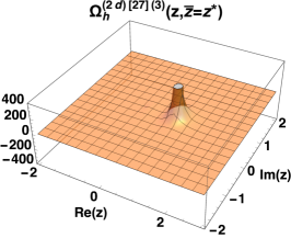
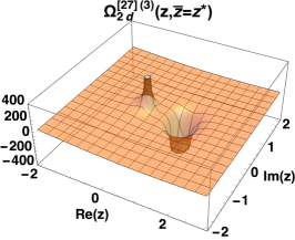
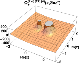
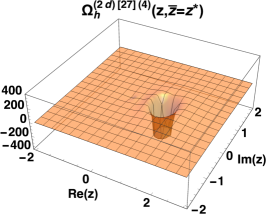
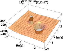
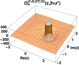
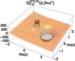
Figure 9: Soft, hard and full wavefunction in the complex plane ${\rm Re}(z)$, ${\rm Im}(z)$. Here we plot the component corresponding to the $27$ colour representation.

6.2 Convergence of the loop expansion of the infrared-renormalized amplitude

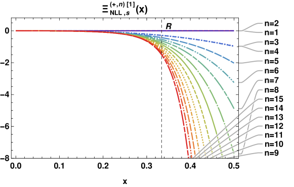
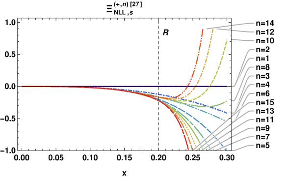
Figure 10: Partial sums of the soft component of the infrared-renormalized amplitude coefficients $\Xi_{\rm NLL,s}^{(+,\ell)}$, up to 15th order, for the singlet (upper plot) and 27 colour representation (lower plot). The dashed vertical line represents the radius of convergence, $R$, determined from the resummed expression.

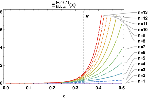
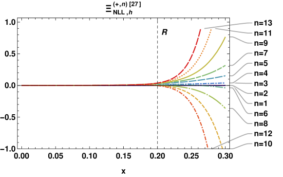
Figure 11: Partial sums of the hard component of the infrared-renormalized amplitude coefficients $\Xi_{\rm NLL,h}^{(+,\ell)}$, up to 13th order, for the singlet (upper plot) and 27 colour representation (lower plot). The dashed vertical line represents the radius of convergence, $R$, determined by the pole closest to $x=0$, using the method of Padé approximants.

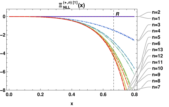
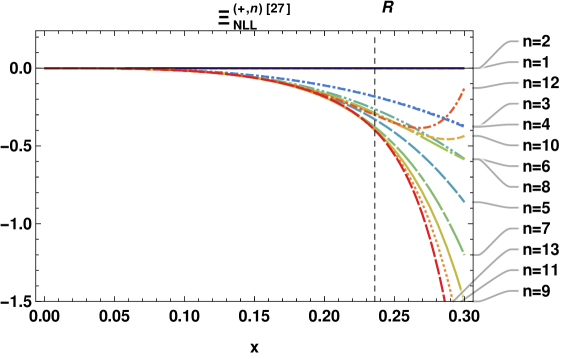
Figure 12: Partial sums of the infrared-renormalized amplitude coefficients $\Xi_{\rm NLL}^{(+,\ell)}$, up to 13th order, for the singlet (upper plot) and the 27 colour representation (lower plot). The dashed vertical line represents the radius of convergence, $R$, determined by the pole closest to $x=0$, using the method of Padé approximants.

Having computed finite contributions to the imaginary part of the amplitude to high loop orders we are in a position to investigate a very interesting theoretical question, namely the convergence properties of the perturbative expansion. Of course, this is done here at a fixed-logarithmic accuracy, namely considering the amplitude as a function of $x\equiv L\,\alpha_{s}/\pi$. The high-energy limit adds an interesting twist to the question of convergence, since within the a priori “perturbative regime” where $\alpha_{s}(\mu^{2})$ is small (recall that $\mu^{2}$ is naturally determined by the momentum transfer $-t$, and we assume $s\gg-t\gg\Lambda_{\rm QCD}^{2}$) high-energy logarithms $L\sim\log|s/t|$ can be arbitrarily large, but then the effective expansion parameter $x\equiv L\,\alpha_{s}/\pi$ becomes large. Thus, while there is no obvious reason why perturbation theory should break down, the question arises whether we can extend the validity of the calculation to large values of the expansion parameter $x$. In Caron-Huot:2017zfo we studied the infrared-divergent part of the amplitude in detail, and proved that these corrections exponentiate in terms of the soft anomalous dimension. We determined the latter to all orders in perturbation theory, and shown that it is an entire function, having an infinite radius of convergence in $x$.

We are now in a position to study the convergence of the infrared-renormalized amplitude ${\cal H}_{\rm NLL}^{(+)}$, which we determined analytically to the 13th order in section 5. For convenience, we introduce the amplitude $\Xi$ and its coefficients $\Xi^{(\ell)}$, defined through

$$\begin{split}{\cal H}_{\rm NLL}^{(+)}&=\frac{i\pi}{L}\,\Xi_{\rm NLL}^{(+)}\,\mathbf{T}_{s-u}^{2}\mathcal{M}^{\mathrm{(tree)}}\,\\ &=\frac{1}{L}\sum_{\ell=1}^{\infty}x^{\ell}{\cal H}_{\rm NLL}^{(+,\ell)}=\frac{i\pi}{L}\sum_{\ell=1}^{\infty}x^{\ell}\,\Xi_{\rm NLL}^{(+,\ell)}\,\mathbf{T}_{s-u}^{2}\mathcal{M}^{\mathrm{(tree)}}\,,\end{split}$$ (184)

such that

$${\cal H}_{\rm NLL}^{(+,\ell)}=i\pi\,\Xi_{\rm NLL}^{(+,\ell)}\,\mathbf{T}_{s-u}^{2}\mathcal{M}^{\mathrm{(tree)}}\,,$$ (185)

cf. eqs. (21) and (22). In the following we will use equivalent definitions also for the soft and hard parts of the infrared-renormalized amplitude coefficients.

Numerical expressions for the coefficients of the infrared-renormalized amplitude $\Xi_{\rm NLL}^{(+,\ell)}$ up to thirteen loops can be obtained starting from the analytic expressions given in the ancillary files, using the relations in eq. (177), and converting the multiple zeta values there into decimal numbers. We arrive at

$$\Xi_{\rm NLL}^{(+)[1]} = -4.959\,x^{3}-0.2283\,x^{4}-9.230\,x^{5}-2.690\,x^{6}-13.13\,x^{7}+1.696\,x^{8}$$ (186)

$$\hskip 5.0pt-\,20.44\,x^{9}+16.54\,x^{10}-35.99\,x^{11}+46.06\,x^{12}-74.05\,x^{13}+\mathcal{O}(x^{14}),$$

$$\Xi_{\rm NLL}^{(+)[27]} = -13.77\,x^{3}-0.6342\,x^{4}-199.2\,x^{5}+381.1\,x^{6}-2826\,x^{7}+9380\,x^{8}$$ (187)

$$\hskip 5.0pt-\,46488\,x^{9}+180393\,x^{10}-797524\,x^{11}+3.239\times 10^{6}\,x^{12}-1.374\times 10^{7}\,x^{13}$$

$$\hskip 5.0pt+\,\mathcal{O}(x^{14}).$$

We consider also the soft and hard contribution to the infrared-renormalized amplitude ${\cal H}_{\rm NLL}^{(+)}$, defined by the two terms in eq. (75). Defining the soft $\Xi_{\rm NLL,s}^{(+)}$ and hard $\Xi_{\rm NLL,h}^{(+)}$, in analogy to eqs. (184) and (185), we can easily obtain a numerical expression for the singlet and 27 colour representation, as in eqs. (186) and (187):

$$\Xi_{\rm NLL,s}^{(+)[1]} = -7.663\,x^{3}-0.2283\,x^{4}-33.73\,x^{5}-78.04\,x^{6}-210.0\,x^{7}-726.9\,x^{8}$$ (188)

$$\hskip 5.0pt-\,2023\,x^{9}-6237\,x^{10}-18605\,x^{11}-55822\,x^{12}-167566\,x^{13}+\mathcal{O}(x^{14}),$$

$$\Xi_{\rm NLL,s}^{(+)[27]} = -15.28\,x^{3}-0.6342\,x^{4}-245.7\,x^{5}+641.8\,x^{6}-4445\,x^{7}+19735\,x^{8}$$ (189)

$$\hskip 5.0pt-\,103863\,x^{9}+507855\,x^{10}-2.566\times 10^{6}\,x^{11}+1.277\times 10^{7}\,x^{12}$$

$$\hskip 10.0pt-\,6.398\times 10^{7}\,x^{13}+\mathcal{O}(x^{14}),\,\,\,\,$$

for the soft part of the infrared-renormalized amplitude, and

$$\Xi_{\rm NLL,h}^{(+)[1]} = 2.705\,x^{3}+24.50\,x^{5}+75.34\,x^{6}+196.9\,x^{7}+728.6\,x^{8}+2003\,x^{9}$$ (190)

$$\hskip 5.0pt+\,6254\,x^{10}+18570\,x^{11}+55869\,x^{12}+167492\,x^{13}+\mathcal{O}(x^{14}),$$

$$\Xi_{\rm NLL,h}^{(+)[27]} = 1.503\,x^{3}+46.45\,x^{5}-260.6\,x^{6}+1619\,x^{7}-10356\,x^{8}+57375\,x^{9}$$ (191)

$$\hskip 5.0pt-\,327462\,x^{10}+1.768\times 10^{6}\,x^{11}-9.527\times 10^{6}\,x^{12}$$

$$\hskip 10.0pt+\,5.024\times 10^{7}\,x^{13}+\mathcal{O}(x^{14}),$$

for its hard part. We plot the partial sums of the soft, hard and full infrared-renormalized amplitude as a function of $x$ respectively in figures 10, 11, and 12.

Considering the all-order resummed expression for the soft component of the infrared-renormalized amplitude in eq. (79), we can immediately conclude that it exhibits a finite radius of convergence. The radius of convergence can be identified as the position of the pole closest to the origin in the complex $x$ plane, which we denote in what follows $R$. Inspecting eq. (79), and in particular the explicit expression for $\hat{\Delta}_{\rm NLL}^{(+)}$ in eq. (72), we see that the soft part of the infrared-renormalized amplitude has poles when the argument of the gamma functions in the numerator equals zero or negative integers. In general poles appear for both positive and negative $x$: this is an important point we shall return to below. The pole closest to the origin is determined by $1-(C_{A}-\mathbf{T}_{t}^{2})\,x=0$, which in turn determines the radius of the convergence of the soft part of the infrared-renormalized amplitude to be $R_{s}=1/(C_{A}-\mathbf{T}_{t}^{2})$ (the subscript “s” refers to the soft part of the infrared-renormalized amplitude). This corresponds to $R_{s}=1/3\simeq 0.333$ for the colour singlet infrared-renormalized amplitude, and $R_{s}=-1/5=-0.2$ for one in the 27 representation. The qualitative picture of convergence of the partial sums as a function of $\ell$ for any $x<R_{s}$, and divergence beyond that point, can indeed be confirmed upon inspecting figure 10.

For the hard contribution to the infrared-renormalized amplitude, and thus also for the complete one, we do not have an all-order expression. Nevertheless, information on the radius of convergence can be extracted from the perturbative expansion by constructing Padé approximants of the infrared-renormalized amplitude. More specifically, we may use the partial sum of the infrared-renormalized amplitude at any order $\ell$ to construct a rational function of $x$, which reproduces the partial sum upon expansion. Here we choose to use Padé approximants of the form:

$$\Xi_{\rm NLL}^{(+)}|_{\text{Pad\'{e}},\ell}=\frac{\sum_{n=3}^{\ell-2}\,a_{n}\,x^{n}}{1+b_{1}\,x+b_{2}\,x^{2}}.$$ (192)

With this definition the Padé approximant has two poles at $x_{\pm}=\big{(}-b_{1}\pm\sqrt{b_{1}^{2}-4b_{2}}\big{)}/(2b_{2})$. The pole closest to the origin provides a prediction for the radius of convergence of the series: $R={\rm min}\{x_{-},x_{+}\}$. Of course, this prediction is expected to be reliable only upon considering sufficiently high orders, where the series approaches its asymptotic regime. The stability of the deduced value for the radius of convergence with respect to the order $\ell$ provides an indication of whether the asymptotic regime is reached.

Before describing the results a further comment is due regarding the sign of $R$. Strictly speaking, the radius of convergence would be the absolute value of $R$. Here, however, we are interested in keeping track also of the sign of the nearest pole, indicating whether the series is (asymptotically) of constant signs, or oscillating. We shall see that both scenarios are realised.

We test this method on the soft part of the infrared-renormalized amplitude, for which the all-order result is known, as discussed above. The results for the singlet and the 27 representation for $N_{c}=3$ are shown in Table 1. We see that in both cases the pole closest to $x=0$ ($x^{[1]}_{\rm s,-}=0.333$ for the singlet and $x^{[27]}_{\rm s,+}=-0.200$ for the 27 representation) approximates very well the exact radius of convergence, $R_{s}=1/(C_{A}-\mathbf{T}_{t}^{2})$.

$\ell$	singlet	27
10	$x^{[1]}_{\rm s,-}=0.335,\quad x^{[1]}_{\rm s,+}=-0.703$	$x^{[27]}_{\rm s,-}=0.472,\quad x^{[27]}_{\rm s,+}=-0.200$
11	$x^{[1]}_{\rm s,-}=0.333,\quad x^{[1]}_{\rm s,+}=-1.053$	$x^{[27]}_{\rm s,-}=0.446,\quad x^{[27]}_{\rm s,+}=-0.200$
12	$x^{[1]}_{\rm s,-}=0.334,\quad x^{[1]}_{\rm s,+}=-1.866$	$x^{[27]}_{\rm s,-}=0.428,\quad x^{[27]}_{\rm s,+}=-0.200$
13	$x^{[1]}_{\rm s,-}=0.333,\quad x^{[1]}_{\rm s,+}=3.911$	$x^{[27]}_{\rm s,-}=0.419,\quad x^{[27]}_{\rm s,+}=-0.200$

Table 1: Table summarising the values of $x=\frac{\alpha_{s}}{\pi}L$ at the poles of the Padé Approximants in eq. (192), considering the soft component of the infrared-renormalized amplitude (indicated by the subscript ${\rm s}$) at orders $\ell=10$ through 13 for the singlet and the 27 representation.

We thus proceed and apply the same method to the hard component of the infrared-renormalized amplitude. The results are summarised in table 2.

$\ell$	singlet	27
10	$x^{[1]}_{\rm h,-}=0.333,\quad x^{[1]}_{\rm h,+}=-0.753$	$x^{[27]}_{\rm h,-}=0.822,\quad x^{[27]}_{\rm h,+}=-0.176$
11	$x^{[1]}_{\rm h,-}=0.332,\quad x^{[1]}_{\rm h,+}=-0.856$	$x^{[27]}_{\rm h,-}=0.096,\quad x^{[27]}_{\rm h,+}=-0.179$
12	$x^{[1]}_{\rm h,-}=0.333,\quad x^{[1]}_{\rm h,+}=-1.258$	$x^{[27]}_{\rm h,-}=-4.392,\quad x^{[27]}_{\rm h,+}=-0.186$
13	$x^{[1]}_{\rm h,-}=0.333,\quad x^{[1]}_{\rm h,+}=-1.244$	$x^{[27]}_{\rm h,-}=-0.02,\quad x^{[27]}_{\rm h,+}=-0.185$

Table 2: Table summarising the values of $x=\frac{\alpha_{s}}{\pi}L$ at the poles of the Padé Approximants in eq. (192), considering the hard component of the infrared-renormalized amplitude (indicated by the subscript ${\rm h}$) at orders $\ell=10$ through 13 for the singlet and the 27 representation.

We observe that for the singlet there is a highly stable nearest pole at $x^{[1]}_{\rm h,-}=0.333$. For the 27 representation, in turn, the stable pole at $x^{[27]}_{\rm h,+}\simeq-0.19$ is not always the one closest to the origin, due to the wide fluctuations of $x^{[27]}_{\rm h,-}$. Finally, for the complete infrared-renormalized amplitude we summarise the results in table 3. Here we find highly stable results: $x^{[1]}_{+}\simeq-0.66$ and $x^{[27]}_{+}\simeq-0.24$.

We conclude that Padé approximants based on partial sums of order $\ell=10$ through $13$, yield fairly stable predictions for the poles. Naturally, ones still finds some fluctuations, which can be attributed to subasymptotic effects, but an overall consistent picture emerges, and we can deduce an approximate radius of convergence in each case from the position of the poles.

$\ell$	singlet	27
10	$x^{[1]}_{-}=1.092,\quad x^{[1]}_{+}=-0.624$	$x^{[27]}_{-}=0.393,\quad x^{[27]}_{+}=-0.236$
11	$x^{[1]}_{-}=1.266,\quad x^{[1]}_{+}=-0.666$	$x^{[27]}_{-}=0.437,\quad x^{[27]}_{+}=-0.237$
12	$x^{[1]}_{-}=1.311,\quad x^{[1]}_{+}=-0.661$	$x^{[27]}_{-}=0.367,\quad x^{[27]}_{+}=-0.238$
13	$x^{[1]}_{-}=1.466,\quad x^{[1]}_{+}=-0.669$	$x^{[27]}_{-}=0.461,\quad x^{[27]}_{+}=-0.239$

Table 3: Table summarising the values of $x=\frac{\alpha_{s}}{\pi}L$ at the poles of the Padé Approximants in eq. (192), considering the full amplitude at orders $\ell=10$ through 13 for the singlet and the 27 representation.

The final results of this analysis are summarised in table 4, where we compare the results for the soft part of the infrared-renormalized amplitude, deduced from the resummed result (which are highly consistent with the Padé approach), with those for the hard component and complete infrared-renormalized amplitude, which are both based solely on the Padé analysis. In the table we also provide an interpretation of the radius of convergence for the full infrared-renormalized amplitude in terms of the analytic dependence on the colour factors $C_{1}$ and $C_{2}$; this will be explained below.

	$x=\frac{\alpha_{s}}{\pi}L$ expansion: convergence radius $R$
Representation	singlet	27
Colour factors	$C_{1}=6$,  $C_{2}=3$	$C_{1}=-2$, $C_{2}=-5$
soft contribution to ${\cal H}_{\rm NLL}^{(+)}$	$1/{C_{2}}=1/3$	$1/{C_{2}}=-1/5$
hard contribution ${\cal H}_{\rm NLL}^{(+)}$	$\sim 0.333$	$\sim-0.19$
Full ${\cal H}_{\rm NLL}^{(+)}$	$-2/{C_{2}}\simeq-0.666$	$1/\big{(}{C_{2}}-\frac{3}{8}{C_{1}}\big{)}\simeq-0.235$

Table 4: Summary table for the radius of convergence $R$ of the expansion of the infrared-renormalized amplitude in powers of $x=\frac{\alpha_{s}}{\pi}L$, determined by identifying the pole closest to $x=0$ using Padé approximants. We use the shorthand notation $C_{1}=(2C_{A}-\mathbf{T}_{t}^{2})$ and $C_{2}=(C_{A}-\mathbf{T}_{t}^{2})$.

The numerical results in the table indicate that the radius of convergence of the full infrared-renormalized amplitude is larger compared to both its soft and hard components. Indeed, better convergence is clearly observed looking at successive orders in the full hard function in figure 12 compared to its soft and hard components in figures 10 and 11, respectively. The interpretation is clear: the pole that limits the convergence of the soft component of the infrared-renormalized amplitude in the resummed expression, eq. (79), exactly cancels against a similar divergence in the hard component, hence the similar values of $R$ for the soft and hard components in table 4. Upon cancelling the leading divergence, a subleading pole is exposed, which becomes the dominant obstruction for convergence of the full amplitude. This is of course another indication that the separation of the finite ${\cal O}(\epsilon^{0})$ terms between the soft and hard regimes is arbitrary; we have already seen that the soft wavefunction cannot approximate the full one away from the soft limit in figures 8 and 9.

Even more interesting is the observation that the sign of the first pole, $R$, which indicates whether the series is asymptotically sign-oscillating ($R<0$) or of constant signs ($R>0$), is negative for the full infrared-renormalized amplitude, while it may be either positive or negative for the separate soft and hard components, as can be seen in table 4. Upon resumming the perturbative expansion of the full infrared-renormalized amplitude, one expects a smooth extrapolation to high energies when taking the centre-of-mass energy large compared to the momentum transfer, $s\gg-t\gg\Lambda_{\rm QCD}^{2}$. Given that the expansion parameter, $x=\frac{\alpha_{s}(-t)}{\pi}\log\frac{s}{-t}$, gets large (and positive) in this limit, smooth extrapolation (of the resummed expression) to high energies can only be consistent with a finite radius of convergence if the series is sign-oscillating, or put in stronger terms: if all the singularities of the resummed infrared-renormalized amplitude are locate away from the positive real axis of $x$. In the example of the soft part of the hard function, singularities appear on the real axis at both positive and negative values. We expect that this would not happen for the full hardfunction. In other words, the singularities present in the resummed soft part of the hard function at positive $x$ must all cancel against similar divergences in the resummed hard part of the hard function. This explains the observations above regarding the radius of convergence of the full hard function versus its soft and hard components, but it applies more generally, also to poles further away from the origin.

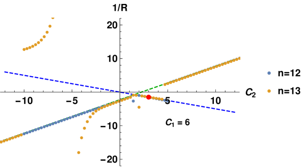
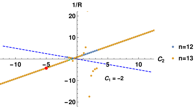
Figure 13: The radius of convergence of the full infrared-renormalized amplitude as a function of the colour operators. In these plots the dots represent the value of $1/R$, for the corresponding value of $C_{1}=(2C_{A}-\mathbf{T}_{t}^{2})$ and $C_{2}=(C_{A}-\mathbf{T}_{t}^{2})$, based on the Padé approximant analysis for $\ell=11$ and $\ell=12$, as indicated in the plots. We superimpose two linear lines, which determine the dependence of $1/R$ on the colour operators, as summarised by eq. (193).

To complete the analysis of the radius of convergence in the full hard function we would now like to interpret the numerical values of $R$ obtained in the Padé-based analysis in terms of the colour structures $C_{1}=(2C_{A}-\mathbf{T}_{t}^{2})$ and $C_{2}=(C_{A}-\mathbf{T}_{t}^{2})$. We start by recalling that for the soft part of the hard function, $R_{s}=1/C_{2}$ depends on $C_{2}$ only. The Padé-based analysis of the 27 colour representation indicates that this is not so for the full hard function. To obtain an analytic expression it proves useful to depart from the actual values of the colour factors corresponding to physically-relevant representations, and simply repeat the Padé approximant analysis for a range of values of $C_{2}$ for a fixed $C_{1}$. To this end we plot in figure 13 the numerical values of $R$ emerging from Padé approximants, as a function of $C_{2}$, for fixed values of $C_{1}$ (we pick $C_{1}=6$ and $C_{1}=-2$, corresponding to the singlet and the 27 representation, for easy reference). More precisely, we display in figure 13 the value of $1/R$ rather than $R$ itself, which makes it easy to recognise the exact linear behaviour. Based on this analysis we deduce the radius of convergence of the full amplitude to be:

$$\begin{split}R=\min\left\{x_{a},x_{b}\right\}\qquad\text{with}&\qquad x_{a}=\frac{1}{C_{2}-\frac{3}{8}C_{1}}=\frac{1}{(C_{A}-\mathbf{T}_{t}^{2})-\frac{3}{8}(2C_{A}-\mathbf{T}_{t}^{2})},\\ &\qquad x_{b}=-\frac{2}{C_{2}}=-\frac{2}{(C_{A}-\mathbf{T}_{t}^{2})}.\end{split}$$ (193)

Returning to the physically-relevant representations, $x_{b}$ end up being closest to the origin ($|x_{b}|<|x_{a}|$) for the singlet representation where $C_{1}^{[1]}=6$, $C_{2}^{[1]}=3$. One then obtains from eq. (193) a radius of convergence of $R=x^{[1]}_{b}\simeq-0.6667$, in accordance with the result in table 4. In turn, $x_{a}$ gives the pole closest to the origin for the 27 representation, namely for $C_{1}^{[27]}=-2$, $C_{2}^{[27]}=-5$, where one obtains from eq. (193) $x^{[27]}_{a}\simeq-0.235$, again, in accordance with table 4.

7 Conclusions

In this paper we completed the perturbative calculation of $2\to 2$ partonic amplitudes at the next-to-leading logarithmic accuracy in the Regge limit to high loop orders. We focused on the previously-unknown even-signature terms, corresponding to the imaginary part of the amplitude, which vanishes at the leading-logarithmic accuracy. Building upon our previous work in ref. Caron-Huot:2017zfo where we determined the infrared singularities, we now computed the finite corrections to the hard amplitude ${\cal H}$, which remain after stripping off, or renormalizing, these singularities. We believe that these results — the soft anomalous dimension and hard functions — together exhaust the physical information contained in these partonic amplitudes.

Our results are based on the well-established BFKL evolution equation in momentum space. Since the even amplitude vanishes at the leading-logarithmic order, only the leading-order BFKL evolution kernel was needed in our calculation, and the final formulae apply equally to quark and gluon amplitudes. We exploited the fact, observed in Caron-Huot:2017zfo , that the two-Reggeon wavefunction is finite. While it is unknown how to diagonalise the BFKL Hamiltonian for arbitrary colour structures beyond the planar limit, we were able to solve the BFKL equation iteratively, treating complementary regions using two different approaches. The first relies on the soft approximation keeping the dimensional regularization parameter finite – the same method we used in ref. Caron-Huot:2017zfo to determine the singularities of the amplitude – while the second relies instead on a computation in exactly two transverse dimensions, which captures general hard momentum configurations where both Reggeons carry momenta of the order of the total momentum transfer $p^{2}=-t$. As shown in eqs. (46) and (50), each separated part of the BFKL-motivated reduced amplitude needs only be calculated to order ${\cal O}(\epsilon^{0})$, and by carefully recombining them we obtained the renormalized amplitude in eq. (174). The result passes several consistency checks and agrees with a direct computation in dimensional regularization, which we performed through five loops.

The central new computation in this paper is the iterative solution of the BFKL equation in two dimensions, leading to a simple algorithm to compute the two-Reggeon wavefunction to any order, presented in section 4. The result lives inside a very rigid space of functions: the $\ell$-loop wavefunction is a linear combination of weight-$\ell$ single-valued harmonic polylogarithms (SVHPLs) of $z$ and $\bar{z}$ with rational coefficients. The algorithm is formulated as an operation on SVHPLs, and it works by producing differential equations in the holomorphic variable $z$ that can be directly integrated in terms of HPLs of $z$, to which we subsequently apply the single-value map to recover the actual wavefunction in terms of SVHPLs of $z$ and $\bar{z}$.

The hard contribution to the infrared-renormalized amplitude ${\cal H}$ computed using the two-dimensional method admits a rather complex structure, and its resummation goes beyond the scope of the present paper. This is to be contrasted with the soft contribution, which we could resum to all orders in terms of gamma functions, eq. (74), which includes singular as well as finite corrections. The number-theoretical content of the hard contribution is interesting: by construction it is restricted to single-valued multi zeta values (see eqs. (169) and (171)). The presence of multi zeta values – which make their first appearance at weight 11 involving a single-valued version Brown:2013gia ; Schnetz:2013hqa of $\zeta_{5,3,3}$ – precludes resummation in terms of gamma functions, so the resummed result would clearly be of different nature to that of the soft contribution.

Having obtained explicit analytic expressions for both the two-Reggeon wavefunction and the infrared-renormalized amplitude ${\cal H}$ to high loop order, it is straightforward to study the results numerically. In section 6 we examine a couple of aspects, first considering the wavefunction and then the infrared-renormalized amplitude. The wavefunction manifests highly regular behaviour as a function of the Reggeon kinematics variables, except for three specific limits. Two of these correspond to the soft limits, $z,\bar{z}\to 0$ and $z,\bar{z}\to\infty$, while the third $z,\bar{z}\to 1$ corresponds to the limit of large internal momentum. The former are described analytically by the soft wavefunction in eq. (61), and by definition the hard wavefunction vanishes there, while a peak at large momentum is present in both the soft and hard wavefunctions. Interestingly, there is a significant – but incomplete – cancellation between these two leading to a more modest peak in the full wavefunction. While this phenomenon does not affect the validity of our results, it would be interesting to independently predict this limit of the wavefunction (extending eq. (183)) which could help find simpler numerical approximations.

Considering the infrared-renormalized amplitude we focused on one interesting problem, namely the convergence of the perturbative expansion. We find that the ${\cal O}(\epsilon^{0})$ infrared-renormalized amplitude has a finite radius of convergence in the expansion parameter $x=L\alpha_{s}/\pi$. For the soft contribution, where we have a resummed analytic expression, eq. (73), this radius of convergence can readily be identified as the first pole of a gamma function, generating asymptotic behaviour $\sim(x(C_{A}-\mathbf{T}_{t}^{2}))^{\ell}$ at high orders, $\ell\to\infty$. The soft contribution is however not physically meaningful on its own, and the complete infrared-renormalized amplitude features a larger radius of convergence, as shown in figure 12 (compare with figures 10 and 11 for the separate soft and hard components). Estimating the convergence radius using Padé approximants for different colour channels, we deduced an empirical formula for the radius of convergence $R$ of the full amplitude in terms of $C_{A}$ and $\mathbf{T}_{t}^{2}$, eq. (193) above. Interestingly, the pole closest to the origin is always on the negative real axis, leading to an asymptotic behaviour of alternating signs. This matches our physical expectation that the resummed expression should smoothly extrapolate to high energies, corresponding to large positive values of $x$, and is similar to what was observed previously for non-global logarithms in ref. Larkoski:2016zzc . It remains for future work to understand the true high-energy (large $x=L\alpha_{s}/\pi$) behaviour.

Let us conclude with a brief summary of the state-of-the-art knowledge of partonic $2\to 2$ scattering amplitudes in the Regge limit. With the completion of this work these amplitudes are known in full to NLL accuracy. The signature odd part, corresponding to the exchange of a single Reggeized gluon was already known, and is given by a Regge pole (3) with two-loop corrections to the trajectory $\alpha^{(2)}_{g}(p^{2})$, and suitable impact factors (the former, in particular, was calculated in Fadin:1995xg ; Fadin:1996tb ; Fadin:1995km ; Blumlein:1998ib ; it can also be extracted from two-loop calculations of $2\to 2$ scattering amplitudes DelDuca:2001gu ). The signature even part, corresponding to a pair of Reggeized gluons, which generate a Regge cut, was determined here. The next frontier is therefore NNLL accuracy. In the signature-odd sector the first step was taken in ref. Caron-Huot:2017fxr , where the non-linear Balitsky-JIMWLK equation was used to compute the Regge cut contribution generated through the evolution of three Reggeized gluons and their mixing with one Reggeon through three loops. It is very interesting, and indeed – using the techniques we developed in the present paper – technically feasible, to compute higher-loop corrections in this tower of logarithms. NNLL corrections in the signature-even sector are in turn simpler and can be deduced from linear BFKL evolution with a NLO kernel Fadin:1995xg ; Fadin:1996tb ; Fadin:1995km ; Blumlein:1998ib , supplemented by suitable impact factors. At N³LL one expects new phenomena such as the mixing of two and four Reggeon states, which can again be computed using the Balitsky-JIMWLK equation.

Finally, beyond their immediate relevance to the the study of the high-energy limit, the results in this paper can be used to check future multi-loop calculations, and ultimately serve as “boundary data” in a bootstrap programme in which amplitudes are deduced using knowledge of the space of functions, analytic properties, symmetries and special kinematic limits. Such a programme was highly successful in the context of ${\cal N}=4$ supersymmetric Yang-Mills theory, see e.g. Caron-Huot:2016owq ; Dixon:2016nkn , but also, more recently in the context of the singularity structure of gauge theories including QCD Almelid:2017qju . In both cases, the high-energy limit served as crucial input.

Appendix A Harmonic polylogarithms

Harmonic polylogarithms (hpls) Remiddi:1999ew extend the natural logarithm $\log z$ with $z\in\mathbb{C}$ to nested integrals. Similarly to the well-known polylogarithms $\mathrm{Li}_{n}(z)$ they are defined recursively namely

$$H_{0,\sigma}(z)=\int_{0}^{z}\mathrm{d}t\frac{H_{\sigma}(t)}{t}\qquad\text{and}\qquad H_{1,\sigma}(z)=\int_{0}^{z}\mathrm{d}t\frac{H_{\sigma}(t)}{1-t}$$ (194)

where $\sigma$ is a “word” of any length made from the letters $\{0,1\}$. The number of indices of a hpl $H(z)$ is called the weight of the function. By means of eq. (194) it corresponds to the number of nested integrals. The recursion is closed by the weight-1 identities

$$H_{0}(z)=\log z\qquad\text{and}\qquad H_{1}(z)=-\log(1-z).$$ (195)

hpls form a shuffle algebra and thus obey shuffle product identities

$$H_{\rho}(z)H_{\sigma}(z)=\sum_{\tau\in\rho\shuffle\sigma}H_{\tau}(z)$$ (196)

where $\rho\shuffle\sigma$ denotes the shuffle of the words $\rho$ and $\sigma$.

The indices of a hpl may be shortened by means of a collapsed notation; one replaces strings of zeros followed by a one according to

$$\underbrace{0,0,\dots,0}_{n\text{ zeros}},1\longrightarrow n+1$$ (197)

for example $H_{0,1,0,0,1,1}(z)\to H_{2,3,1}(z)$. In the collapsed notation the number of indices is referred to as the depth of the function (while their sum now equals the weight).

Depending on the context it may be useful to view the hpls as nested sums. One commonly used definition is

$$H_{\sigma}(z)=\sum_{j=1}^{\infty}z^{j}Z_{j}(\sigma)$$ (198)

with

$$Z_{j}(a,\sigma)=\frac{1}{j^{a}}\sum_{i=2}^{j}Z_{i-1}(\sigma)\qquad\text{and}\qquad Z_{j}(1)=1/j$$ (199)

where we assume the collapsed notation. Note that the aforementioned depth is equal to the number of nested sums.

The Taylor series of hpls, defined by eq. (194), whose rightmost index is non-zero, is given by eq. (198) with (199). Trailing zeros in the indices of a hpl point to logarithmic divergences at $z=0$. The $\log z=H_{0}(z)$ terms can be exposed using the shuffle algebra; one considers

$$H_{\sigma}(z)H_{0}(z)=H_{\sigma,0}(z)+\ldots+H_{0,\sigma}(z)$$ (200)

and solves for $H_{\sigma,0}(z)$. This procedure can be applied recursivly until all trailing zeros are removed. Hence, hpls can always be written as a series in $z$ and $\log z$.

For arguments between 0 and 1 hpls yield real values. They show branch cuts on the real axis where $z\in[1,\infty)$ and are thus multi-valued functions.

Appendix B Single-valued harmonic polylogarithms

Single-valued harmonic polylogarithms (svhpls) Brown:2004ugm are the class of all branch cut-free, single-valued, combinations of hpls. Their construction is somewhat involved and we will only provide a short summary here. Further details can be found in e.g. refs. Pennington:2012zj ; Dixon:2012yy ; DelDuca:2013lma .

svhpls are functions of a complex variable $z$ and its complex conjugate $\bar{z}$. They correspond to the linear combinations of $H_{\sigma}(z)H_{\sigma^{\prime}}(\bar{z})$ that solve

$$\frac{\mathrm{d}}{\mathrm{d}{z}}\mathcal{L}_{0,\sigma}(z,\bar{z})=\frac{\mathcal{L}_{\sigma}(z,\bar{z})}{z}\qquad\text{and}\qquad\frac{\mathrm{d}}{\mathrm{d}{z}}\mathcal{L}_{1,\sigma}(z,\bar{z})=\frac{\mathcal{L}_{\sigma}(z,\bar{z})}{1-z}$$ (201)

and obey the boundary conditions Pennington:2012zj

$$\mathcal{L}_{\varnothing}(z,\bar{z})=1,\qquad\mathcal{L}_{\vec{0}_{n}}(z,\bar{z})=\log^{n}(z\bar{z})/n!\qquad\text{and}\qquad\lim_{z\to 0}\mathcal{L}_{\sigma\neq\vec{0}_{n}}(z,\bar{z})=0.$$ (202)

For the explicit construction one typically defines two alphabets $\{x_{0},x_{1}\}$ and $\{y_{0},y_{1}\}$ and the corresponding sets of all words $X^{*}$ and $Y^{*}$ formed from the respective alphabet. The letters of the former alphabet directly translate to $\{0,1\}$ when they appear as the indices of a (SV)HPL. The letters $y_{0},y_{1}$ are related to $x_{0},x_{1}$ via

$$y_{0} =x_{0}$$ (203)

$$\tilde{Z}(y_{0},y_{1})y_{1}\tilde{Z}(y_{0},y_{1})^{-1} =Z(x_{0},x_{1})^{-1}x_{1}Z(x_{0},x_{1})$$ (204)

where $Z$ is the so-called Drinfeld associator. It is defined as the generating series

$$Z(x_{0},x_{1})=\sum_{\sigma\in X^{*}}H_{\sigma}(1)\sigma\qquad\text{and}\qquad\tilde{Z}(y_{0},y_{1})=\sum_{\sigma\in Y^{*}}H_{\phi(\sigma)}(1)\tilde{\sigma}$$ (205)

where the “tilde” operation reverses words and $\phi$ maps $y_{i}\to x_{i}$. The values of the hpls at $z=1$ in the definition (205) are regularised by the shuffle algebra. Eq. (204) can be solved iteratively for $y_{1}$.

The svhpls can then be extracted from the product of another two generating series

$$\sum_{\sigma\in X^{*}}\mathcal{L}_{\sigma}(z,\bar{z})=L_{X}(z)\tilde{L}_{Y}(\bar{z})$$ (206)

where

$$L_{X}(z)=\sum_{\sigma\in X^{*}}H_{\sigma}(z)\sigma\qquad\text{and}\qquad\tilde{L}_{Y}(\bar{z})=\sum_{\sigma\in Y^{*}}H_{\phi(\sigma)}(\bar{z})\tilde{\sigma}$$ (207)

with “tilde” and $\phi$ defined below eq.(205).

svhpls obey the same shuffle product as hpls (196), namely

$$\mathcal{L}_{\rho}(z,\bar{z})\mathcal{L}_{\sigma}(z,\bar{z})=\sum_{\tau\in\rho\shuffle\sigma}\mathcal{L}_{\tau}(z,\bar{z}).$$ (208)

B.1 Holomorphic part and single-value map

svhpls are uniquely fixed by their holomorphic part (i.e. their functional dependence on $z$) and the requirement of single-valuedness. We define the holomorphic part of a function $\psi(z,\bar{z})$ as the limit

$$\psi^{(h)}(z)=\psi(z,0)\big{|}_{\log\bar{z}\to 0}.$$ (209)

For a given linear combination of svhpls taking this limit simply amounts to replacing $\mathcal{L}_{\sigma}(z,\bar{z})\to H_{\sigma}(z)$.

The dependence on $\bar{z}$ is reconstructed by the single-value map

$$\mathbf{s}\left(\psi^{(h)}(z)\right)=\psi(z,\bar{z})$$ (210)

which is discussed in detail in refs. Brown:2013gia ; DelDuca:2016lad . Again, we restrict ourselves here to stating the (obvious) replacement rule $H_{\sigma}(z)\to\mathcal{L}_{\sigma}(z,\bar{z})$ which generates the corresponding single-valued expression from a linear combination of hpls of $z$. As the action of the Hamiltonian $\hat{H}_{\mathrm{2d,i}}$ (91a) removes constant terms from the wavefunction prior to integration we shall not discuss this aspect in the context of eqs. (209) and (210) here. The interested reader is referred to the above references.

B.2 Variable transformations

svhpls obey relations under certain variable transformations. For the most part they are, in some sense, the same relations that apply to hpls due to the single-value map discussed above in appendix B.1. While the latter are much better documented (for an overview we recommend ref. Maitre:2005uu ) we struggled to find a comprehensive list for svhpls which motivated this appendix.

In section 4.3 we transform $z\to 1/z$ and $z\leftrightarrow\bar{z}$ to account for the symmetries of the two-dimensional wavefunction. In addition, we consider $z\to 1-z$ in section 5.2 to facilitate the “last integration”. Let us discuss the latter transformation in detail.

At the level of hpls it is straightforward to find relations under $z\to 1-z$. Effectively, the transformation moves the lower limit of the integral definition (194) from zero to one. Consider the weight-$w$ hpls with argument $1-z$

$$H_{0,a_{2},\dots,a_{w}}(1-z) =\int_{0}^{1-z}\frac{\mathrm{d}t}{t}H_{a_{2},\dots,a_{w}}(t)$$

$$=\int_{0}^{1}\frac{\mathrm{d}t}{t}H_{a_{2},\dots,a_{w}}(t)-\int_{1-z}^{1}\frac{\mathrm{d}t}{t}H_{a_{2},\dots,a_{w}}(t)$$

$$=H_{0,a_{2},\dots,a_{w}}(1)-\int_{0}^{z}\frac{\mathrm{d}t}{1-t}H_{a_{2},\dots,a_{w}}(1-t)$$ (211)

and

$$H_{1,a_{2},\dots,a_{w}}(1-z) =\int_{0}^{1-z}\frac{\mathrm{d}t}{1-t}H_{a_{2},\dots,a_{w}}(t)$$

$$=\int_{0}^{1}\frac{\mathrm{d}t}{1-t}H_{a_{2},\dots,a_{w}}(t)-\int_{1-z}^{1}\frac{\mathrm{d}t}{1-t}H_{a_{2},\dots,a_{w}}(t)$$

$$=H_{1,a_{2},\dots,a_{w}}(1)-\int_{0}^{z}\frac{\mathrm{d}t}{t}H_{a_{2},\dots,a_{w}}(1-t)$$ (212)

with

$$H_{0}(1-z)=-H_{1}(z)\quad\text{and}\quad H_{1}(1-z)=-H_{0}(z).$$ (213)

Since the hpls inside the integrals in eqs. (211) and (212) are of weight $w-1$ this defines a recursive prescription of how to write any hpl of $1-z$ in terms of hpls of $z$.

By means of the holomorphic part of svhpls and the single-value map, see appendix B.1, these relations can be applied to svhpls. However, it is also possible to solve the recursion and write the answer directly as a sum. We find

$$\mathcal{L}_{a_{1},\dots,a_{w}}(1-z,1-\bar{z})=\sum_{j=0}^{w}(-1)^{j}\mathcal{L}_{\tilde{a}_{1},\dots,\tilde{a}_{j}}(z,\bar{z})\mathcal{L}_{a_{j+1},\dots,a_{w}}(1,1)$$ (214)

with the “$\sim$” operation swapping the indices $0\leftrightarrow 1$.

Similarly, on can derive identities for the transformation $z\to 1/z$, $\bar{z}\to 1/\bar{z}$. Again, the recursion can be solved and the resulting formula is simply yet slightly awkward to write out. To do so we define $n_{0}(\sigma)$ ($n_{1}(\sigma)$) to count the number zeros (ones) in the indices $\sigma$ and $\hat{s}_{1\to 0+1}$ to split $\mathcal{L}_{\sigma}(z,\bar{z})$ into a sum of $2^{n_{1}(\sigma)}$ svhpls according to the index rule $1\to 0+1$. For example,

$$\hat{s}_{1\to 0+1}\left[\mathcal{L}_{1,0,0,1,0}(z,\bar{z})\right]=\\ \mathcal{L}_{0,0,0,0,0}(z,\bar{z})+\mathcal{L}_{0,0,0,1,0}(z,\bar{z})+\mathcal{L}_{1,0,0,0,0}(z,\bar{z})+\mathcal{L}_{1,0,0,1,0}(z,\bar{z})$$ (215)

Then

$$\mathcal{L}_{a_{1},\dots,a_{w}}\left(\frac{1}{z},\frac{1}{\bar{z}}\right)=\sum_{j=0}^{w}(-1)^{n_{0}(a_{1},\dots,a_{j})}\hat{s}_{1\to 0+1}\left[\mathcal{L}_{a_{1},\dots,a_{j}}(z,\bar{z})\right]\mathcal{L}_{a_{j+1},\dots,a_{w}}(\infty,\infty).$$ (216)

The values of svhpls at $z,\bar{z}\to\infty$ are related to the values at $z,\bar{z}=1$ by yet another transformation: $z\to z/(z-1)$.

$$\mathcal{L}_{a_{1},\dots,a_{w}}\left(\frac{z}{z-1},\frac{\bar{z}}{\bar{z}-1}\right)=(-1)^{n_{1}(a_{1},\dots,a_{w})}\hat{s}_{0\to 0+1}\left[\mathcal{L}_{a_{1},\dots,a_{w}}(z,\bar{z})\right]$$ (217)

with $\hat{s}_{0\to 0+1}$ defined like $\hat{s}_{1\to 0+1}$ (210) but based on the index rule $0\to 0+1$. This last step is not strictly necessary but it reduces the amount of data needed to apply these kinds of transformations to a list of svhpls at $z,\bar{z}=1$.

Lastly, let us examine the transformation $z\leftrightarrow\bar{z}$ and how to related an svhpl $\mathcal{L}_{\sigma}(\bar{z},z)$ to (a sum of) svhpls $\mathcal{L}_{\sigma_{i}^{\prime}}(z,\bar{z})$. The easy yet computationally heavy way is to translate $\mathcal{L}_{\sigma}(z,\bar{z})$ to hpls, swap $z\leftrightarrow\bar{z}$, extract the holomorphic part by means of eq. (209) and finally apply $\mathbf{s}$ (210). For svhpls of weight less or equal to five this might be adequate but at higher weights it becomes inefficient due to the large size of expressions that the translation to hpls causes. Like in the above examples this step can be avoided altogether.

The procedure relies on knowing the functional dependence of $y_{1}$ on the $x_{i}$, cf. eq. (204). Consider the weight-$n$ svhpl $\mathcal{L}_{\sigma}(z,\bar{z})$ with $\sigma=\sigma_{1},\dots,\sigma_{n}$ and swap $z\leftrightarrow\bar{z}$. Then

$$\mathcal{L}_{\sigma}(\bar{z},z)=\mathcal{L}_{\tilde{\sigma}}(z,\bar{z})+\sum_{i=4}^{|\sigma|}\sum_{j=0}^{|\sigma|-i}y1(\sigma_{j},\dots,\sigma_{i+j})\mathcal{L}_{\underbrace{\scriptstyle\sigma_{1},\dots,\sigma_{j-1}}_{(A)},\underbrace{\scriptstyle\sigma_{i+j+1},\dots,\sigma_{n}}_{(B)},1}$$ (218)

where the “tilde” map was defined below eq. (205) and $y1(\sigma)$ is the coefficient of the product of $x_{0}$ and $x_{1}$ corresponding to $\sigma$, e.g. if $\sigma=1,1,0,1,0$ then $y1(\sigma)$ is the coefficient of $x_{1}x_{1}x_{0}x_{1}x_{0}$. The indices (A) in eq. (218) only appear if $j-1\geq 1$ and likewise (B) if $i+j+1\leq n$.

References

- (1) E. A. Kuraev, L. N. Lipatov and V. S. Fadin, The Pomeranchuk Singularity in Nonabelian Gauge Theories, Sov. Phys. JETP 45 (1977) 199–204.
- (2) I. I. Balitsky and L. N. Lipatov, The Pomeranchuk Singularity in Quantum Chromodynamics, Sov. J. Nucl. Phys. 28 (1978) 822–829.
- (3) L. N. Lipatov, The Bare Pomeron in Quantum Chromodynamics, Sov. Phys. JETP 63 (1986) 904–912.
- (4) A. H. Mueller, Soft gluons in the infinite momentum wave function and the BFKL pomeron, Nucl. Phys. B415 (1994) 373–385.
- (5) A. H. Mueller and B. Patel, Single and double BFKL pomeron exchange and a dipole picture of high-energy hard processes, Nucl. Phys. B425 (1994) 471–488, [hep-ph/9403256].
- (6) R. C. Brower, J. Polchinski, M. J. Strassler and C.-I. Tan, The Pomeron and gauge/string duality, JHEP 12 (2007) 005, [hep-th/0603115].
- (7) I. Moult, M. P. Solon, I. W. Stewart and G. Vita, Fermionic Glauber Operators and Quark Reggeization, 1709.09174.
- (8) I. Balitsky, Operator expansion for high-energy scattering, Nucl. Phys. B463 (1996) 99–160, [hep-ph/9509348].
- (9) I. Balitsky, Factorization for high-energy scattering, Phys. Rev. Lett. 81 (1998) 2024–2027, [hep-ph/9807434].
- (10) Y. V. Kovchegov, Small x F(2) structure function of a nucleus including multiple pomeron exchanges, Phys. Rev. D60 (1999) 034008, [hep-ph/9901281].
- (11) J. Jalilian-Marian, A. Kovner, L. D. McLerran and H. Weigert, The Intrinsic glue distribution at very small x, Phys. Rev. D55 (1997) 5414–5428, [hep-ph/9606337].
- (12) J. Jalilian-Marian, A. Kovner, A. Leonidov and H. Weigert, The Wilson renormalization group for low x physics: Towards the high density regime, Phys. Rev. D59 (1998) 014014, [hep-ph/9706377].
- (13) E. Iancu, A. Leonidov and L. D. McLerran, The Renormalization group equation for the color glass condensate, Phys. Lett. B510 (2001) 133–144, [hep-ph/0102009].
- (14) M. G. Sotiropoulos and G. F. Sterman, Color exchange in near forward hard elastic scattering, Nucl. Phys. B419 (1994) 59–76, [hep-ph/9310279].
- (15) G. P. Korchemsky, On Near forward high-energy scattering in QCD, Phys. Lett. B325 (1994) 459–466, [hep-ph/9311294].
- (16) I. A. Korchemskaya and G. P. Korchemsky, Evolution equation for gluon Regge trajectory, Phys. Lett. B387 (1996) 346–354, [hep-ph/9607229].
- (17) I. A. Korchemskaya and G. P. Korchemsky, High-energy scattering in QCD and cross singularities of Wilson loops, Nucl. Phys. B437 (1995) 127–162, [hep-ph/9409446].
- (18) V. Del Duca and E. W. N. Glover, The High-energy limit of QCD at two loops, JHEP 10 (2001) 035, [hep-ph/0109028].
- (19) V. Del Duca, G. Falcioni, L. Magnea and L. Vernazza, High-energy QCD amplitudes at two loops and beyond, Phys. Lett. B732 (2014) 233–240, [1311.0304].
- (20) V. Del Duca, G. Falcioni, L. Magnea and L. Vernazza, Analyzing high-energy factorization beyond next-to-leading logarithmic accuracy, JHEP 02 (2015) 029, [1409.8330].
- (21) V. Del Duca, C. Duhr, E. Gardi, L. Magnea and C. D. White, An infrared approach to Reggeization, Phys. Rev. D85 (2012) 071104, [1108.5947].
- (22) V. Del Duca, C. Duhr, E. Gardi, L. Magnea and C. D. White, The Infrared structure of gauge theory amplitudes in the high-energy limit, JHEP 12 (2011) 021, [1109.3581].
- (23) S. Caron-Huot, When does the gluon reggeize?, JHEP 05 (2015) 093, [1309.6521].
- (24) S. Caron-Huot, E. Gardi and L. Vernazza, Two-parton scattering in the high-energy limit, JHEP 06 (2017) 016, [1701.05241].
- (25) S. Caron-Huot, E. Gardi, J. Reichel and L. Vernazza, Infrared singularities of QCD scattering amplitudes in the Regge limit to all orders, JHEP 03 (2018) 098, [1711.04850].
- (26) F. C. S. Brown, Polylogarithmes multiples uniformes en une variable, Compt. Rend. Math. 338 (2004) 527–532.
- (27) F. Brown, Single-valued Motivic Periods and Multiple Zeta Values, SIGMA 2 (2014) e25, [1309.5309].
- (28) F. Chavez and C. Duhr, Three-mass triangle integrals and single-valued polylogarithms, JHEP 11 (2012) 114, [1209.2722].
- (29) O. Schnetz, Graphical functions and single-valued multiple polylogarithms, Commun. Num. Theor. Phys. 08 (2014) 589–675, [1302.6445].
- (30) J. Pennington, The six-point remainder function to all loop orders in the multi-Regge limit, JHEP 01 (2013) 059, [1209.5357].
- (31) L. J. Dixon, C. Duhr and J. Pennington, Single-valued harmonic polylogarithms and the multi-Regge limit, JHEP 10 (2012) 074, [1207.0186].
- (32) V. Del Duca, L. J. Dixon, C. Duhr and J. Pennington, The BFKL equation, Mueller-Navelet jets and single-valued harmonic polylogarithms, JHEP 02 (2014) 086, [1309.6647].
- (33) L. J. Dixon, J. M. Drummond, C. Duhr and J. Pennington, The four-loop remainder function and multi-Regge behavior at NNLLA in planar N = 4 super-Yang-Mills theory, JHEP 06 (2014) 116, [1402.3300].
- (34) V. Del Duca, S. Druc, J. Drummond, C. Duhr, F. Dulat, R. Marzucca et al., Multi-Regge kinematics and the moduli space of Riemann spheres with marked points, JHEP 08 (2016) 152, [1606.08807].
- (35) V. Del Duca, S. Druc, J. Drummond, C. Duhr, F. Dulat, R. Marzucca et al., The seven-gluon amplitude in multi-Regge kinematics beyond leading logarithmic accuracy, JHEP 06 (2018) 116, [1801.10605].
- (36) O. Almelid, C. Duhr, E. Gardi, A. McLeod and C. D. White, Bootstrapping the QCD soft anomalous dimension, JHEP 09 (2017) 073, [1706.10162].
- (37) L. J. Dixon, E. Herrmann, K. Yan and H. X. Zhu, Soft gluon emission at two loops in full color, 1912.09370.
- (38) Yu. L. Dokshitzer and G. Marchesini, Soft gluons at large angles in hadron collisions, JHEP 01 (2006) 007, [hep-ph/0509078].
- (39) S. Catani, The Singular behavior of QCD amplitudes at two loop order, Phys. Lett. B427 (1998) 161–171, [hep-ph/9802439].
- (40) J. Carter and G. Heinrich, SecDec: A general program for sector decomposition, Comput. Phys. Commun. 182 (2011) 1566–1581, [1011.5493].
- (41) S. Borowka, G. Heinrich, S. Jahn, S. P. Jones, M. Kerner and J. Schlenk, Numerical evaluation of two-loop integrals with pySecDec, Acta Phys. Polon. Supp. 11 (2018) 375, [1712.05755].
- (42) G. F. Sterman, Partons, factorization and resummation, TASI 95, in Theoretical Advanced Study Institute in Elementary Particle Physics (TASI 95): QCD and Beyond, pp. 327–408, 6, 1995. hep-ph/9606312.
- (43) J. C. Collins, D. E. Soper and G. F. Sterman, Factorization of Hard Processes in QCD, Adv. Ser. Direct. High Energy Phys. 5 (1989) 1–91, [hep-ph/0409313].
- (44) S. M. Aybat, L. J. Dixon and G. F. Sterman, The Two-loop soft anomalous dimension matrix and resummation at next-to-next-to leading pole, Phys. Rev. D74 (2006) 074004, [hep-ph/0607309].
- (45) G. F. Sterman and M. E. Tejeda-Yeomans, Multiloop amplitudes and resummation, Phys. Lett. B 552 (2003) 48–56, [hep-ph/0210130].
- (46) E. Gardi and L. Magnea, Factorization constraints for soft anomalous dimensions in QCD scattering amplitudes, JHEP 03 (2009) 079, [0901.1091].
- (47) T. Becher and M. Neubert, Infrared singularities of scattering amplitudes in perturbative QCD, Phys. Rev. Lett. 102 (2009) 162001, [0901.0722].
- (48) T. Becher and M. Neubert, On the Structure of Infrared Singularities of Gauge-Theory Amplitudes, JHEP 06 (2009) 081, [0903.1126].
- (49) O. Almelid, C. Duhr and E. Gardi, Three-loop corrections to the soft anomalous dimension in multileg scattering, Phys. Rev. Lett. 117 (2016) 172002, [1507.00047].
- (50) M. D. Schwartz and H. X. Zhu, Nonglobal logarithms at three loops, four loops, five loops, and beyond, Phys. Rev. D90 (2014) 065004, [1403.4949].
- (51) A. J. Larkoski, I. Moult and D. Neill, The Analytic Structure of Non-Global Logarithms: Convergence of the Dressed Gluon Expansion, JHEP 11 (2016) 089, [1609.04011].
- (52) V. S. Fadin, M. I. Kotsky and R. Fiore, Gluon Reggeization in QCD in the next-to-leading order, Phys. Lett. B359 (1995) 181–188.
- (53) V. S. Fadin, R. Fiore and M. I. Kotsky, Gluon Regge trajectory in the two loop approximation, Phys. Lett. B387 (1996) 593–602, [hep-ph/9605357].
- (54) V. S. Fadin, R. Fiore and A. Quartarolo, Reggeization of quark quark scattering amplitude in QCD, Phys. Rev. D53 (1996) 2729–2741, [hep-ph/9506432].
- (55) J. Blumlein, V. Ravindran and W. L. van Neerven, On the gluon Regge trajectory in O alpha-s**2, Phys. Rev. D58 (1998) 091502, [hep-ph/9806357].
- (56) S. Caron-Huot, L. J. Dixon, A. McLeod and M. von Hippel, Bootstrapping a Five-Loop Amplitude Using Steinmann Relations, Phys. Rev. Lett. 117 (2016) 241601, [1609.00669].
- (57) L. J. Dixon, J. Drummond, T. Harrington, A. J. McLeod, G. Papathanasiou and M. Spradlin, Heptagons from the Steinmann Cluster Bootstrap, JHEP 02 (2017) 137, [1612.08976].
- (58) E. Remiddi and J. A. M. Vermaseren, Harmonic polylogarithms, Int. J. Mod. Phys. A15 (2000) 725–754, [hep-ph/9905237].
- (59) D. Maitre, HPL, a mathematica implementation of the harmonic polylogarithms, Comput. Phys. Commun. 174 (2006) 222–240, [hep-ph/0507152].