A Thousand Words are Worth More Than One Recording: NLP Based Speaker Change Point Detection

Abstract

Speaker Diarization (SD) consists of splitting or segmenting an input audio burst according to speaker identities. In this paper, we focus on the crucial task of the SD problem which is the audio segmenting process and suggest a solution for the Change Point Detection (CPD) problem. We empirically demonstrate the negative correlation between an increase in the number of speakers and the Recall and F1-Score measurements. This negative correlation is shown to be the outcome of a massive experimental evaluation process, which accounts its superiority to recently developed voice based solutions. In order to overcome the number of speakers issue, we suggest a robust solution based on a novel Natural Language Processing (NLP) technique, as well as a metadata features extraction process, rather than a vocal based alone. To the best of our knowledge, we are the first to tackle this variant on the SD problem (or CPD) from the intelligent NLP standpoint, and with a dataset in the Hebrew language which is an issue in its own right. We empirically show, based on two distinct datasets, that our method is abled to accurately identify the CPD’s in an audio burst with 82.12% and 89.02% of success in the Recall and F1-score measurements.

1 Introduction

Alice asks Bob to make a statement. Two days later, she decides to go over his answers because she feels she missed some details. As Bob likes to talk, and since Alice went over the details carefully, the recorded statement lasted more than an hour. Luckily, Alice has access to a diarization system that allows her to isolate the segments in which Bob was talking. A Speaker Diarization (SD) system aims to answer the question “who spoke when?” for a given audio burst, by identifying the start and ending time of each segment, as well as the speaker’s identity. Speaker Diarization [57, 58, 63] has many applications in real world: speaker turn analysis, speaker indexing, speech recognition with speaker identification, and diarizing meeting and lectures [44, 47]. Given the scope of the diarization problem (e.g., unknown number of speakers, supporting multiple languages, voice quality), SD is considered as a hard research problem, that has attracted numerous researcher’s attention for more than a decade  [60, 52, 27, 15, 21, 13, 11, 23].

A typical SD system can be divided into a number of components: (i) a speech segmentation module, which detects and removes the non-speech parts, then divides the input into small segments; (ii) An embedding extraction module, where speaker-discriminative embeddings such as speaker factors or Mel Frequency Cepstral Coefficient (MFCC) vectors  [54] are extracted from each segment; (iii) a clustering module, which determines the number of speakers, and (iv) a classification module that assigns a speaker identity for each segment. Since our objective is to detect the time points at which the identity of the speaker changes, we actually solve the Change Point Detection problem (CPD)  [8, 10, 19]. In statistical analysis, the CPD problem consists of identifying locations on time when the probability distribution of a stochastic process or sequential data changes. More generally, the CPD problem detects whether or not a change has occurred, and identifies the times when these changes took place. One of the main CPD applications is the detection of anomalous behavior, which is well known in literature as the Anomaly Detection (AD) problem  [28, 25]. In a typical anomaly detection system, a clustering algorithm is needed to identify the set of outliers  [28]. Since the CPD problem can be easily framed as an AD, this work can be seen as an AD problem as well, because the change points in our data are exactly the anomalies that we are looking for.

This paper presents the benefits of tackling the CPD problem from a textual standpoint. We introduce a new model for the CPD (or AD) problem called TSCPD, which stands for Textual Speaker Change Point Detection. We focus on the first task (i.e., division into segments), and empirically show the negative correlation between an increase in the number of speakers and the state-of-the-art solution quality. Thus, we propose a transition from the vocal domain to the textual domain by running a Speech-2-Text algorithm over the dataset on the vocal signals. One of the main contributions of the TSCPD approach, is that it yields a robust model, which is only trained by a neural network once over the dataset, but then fits for other datasets with speakers who did not appear in the dataset used to train the model at all (see Section 5.2). In addition, our model shows robustness on other Speech-2-Text engine and new speakers (see Section 5.4). More specifically, we present an NLP-based hybrid solution for the CPD problem, as well as the development process of a deep learning based approach such that given an audio burst, our method determines all of the points in time in which the speaker identity has changed.

To the best of our knowledge, we are the first to propose an intelligent NLP based solution that (I) tackles the CPD problem with a dataset in Hebrew (discussed in depth in Section 2), and (II) solves the CPD variant of the SD problem. Our empirical experimental evaluation process (Section 5) shows that the transition from voice analysis to the NLP approach, can accurately identify the CPD’s for a given multi-participant conversation with 82.12% success reflected by the model’s Recall measurement. Moreover, our speakers-number-independent approach outperforms recently voice-based solutions [63, 57] to the original SD problem, which are based on the D-vectors [26, 20] extracted from the speech signal and clearly depend on the number of speakers. In addition, while the number of speakers and their differences in pronunciation and intonation are a critical issue in these voice-based solutions, we show that our approach remains robust to these vocal elements.

The remainder of this paper is structured as follows: Section 2 surveys related work on the famous SD problem, clustering algorithms and the difficulties of coping with datasets in the Hebrew language; Section 3 provides a brief background on the dataset and a description of the feature encoding process; Section 4 presents the methodology employed in this work, and our Neural Network based approach; Section 5 provides a fine-grained experimental evaluation framework, and Section 6 concludes and summarizes this paper. For ease of reading, we provide a list of abbreviations in Table 1.

Abbreviation Meaning SD Speaker Diarization CPD Change Point Detection NLP Natural Language Processing AD Anomaly Detection TSCPD Textual Speaker Change Point Detection SV Speaker Verification SCD Speaker Change Detection UIS-RNN Unbounded Interleaved-State Recurrent Neural Networks
Table 1: List of Abbreviations

2 Related Work

The SD problem and its variants have been discussed in numerous research papers for the last few years  [58, 63, 57, 20, 3, 12]. It is striking that most works on the SD problem have tackled it from the speech signal point of view. The model presented in [63], aims to solve the SD problem through a supervised speaker diarization approach, termed Unbounded Interleaved-State Recurrent Neural Networks (UIS-RNN). The UIS-RNN approach is designed to solve the SD problem by learning the extracted speaker-discriminative embeddings (a.k.a. D-vectors [26, 20]) from input utterances, where each individual speaker is modeled by a parameter-sharing RNN, whereas the RNN states for different speakers interleave in the time domain. This RNN is naturally integrated with a distance-dependent Chinese Restaurant Process (ddCRP,  [6, 1]) to accommodate an unknown number of speakers. This UIS-RNN model draws on the construction in [57] of D-vectors, whose authors developed both a Text-Dependent and a Text-Independent Speaker Verification (TD-SV, TI-SV) method for the Speaker Verification (SV) problem, based on a new loss function called Generalized End-to-End (GE2E) loss, which makes the training of speaker verification models more efficient than Tuple-based End-to-End (TE2E, [20]) loss function. In this GE2E method, the training process consists of building training batches from $N$ different speakers and $M$ speech utterances for each of the $N$ speakers at each step, so that each speaker utterance is represented as a feature-vector. Then, the features extracted from each speaker utterance are fed into a Long-Short-Term-Memory (LSTM [22]) Neural Network. Next, a linear layer is connected to the last LSTM layer as an additional transformation of the last frame response of the network. The outcome of the training process is an embedding vector (D-vector) for each speaker utterance, which is defined as the L2 normalization of the neural network output. By contrast, the model presented in [16] suggested using X-vectors for the online SD problem, by performing qualitative modifications of the UIS-RNN [63] to improve learning efficiency and the overall diarization performance. In particular, they introduced a loss function called Sample Mean Loss (SML), as well as a modelling of speaker turn behavior, which involved devising an analytical expression to compute the probability of a new speaker joining the conversation.

We show that these state-of-the-art SD systems [63, 57] suffer from a dramatically lower recall as the number of speakers in the dataset increase. Clearly, this dependency poses a massive challenge, especially since the number of speakers in a given audio burst is typically unknown in advance. This incomplete information forces a typical SD system to rely on the performance of clustering tools  [34, 51, 50, 36] to determine the number of speakers in a given audio burst. Assuming that a clustering process correctly detects how many speakers are in a given audio burst, an SD systems quality is assessed in terms of the assignment of speaker identities to each segment in the audio burst. The two other main challenges in SD are language variants, which are manifested in the speaker pronunciation and intonation, and the sound quality. All of these, impact the speech signal analysis.

The solutions in [63, 57, 20] have tackled the SD\SV problems in terms of the speech signal. Other examples related to SD and the speech signal are presented in [31] that described a SD method based on the separation of under-determined speech mixtures, where the number of speakers was greater than the number of microphones; The authors in [7] proposed an algorithm to estimate the number of speakers, using reliability information to obtain robust estimation results in adverse acoustic scenarios, and estimating the individual probability distributions describing the location of each speaker using convex geometry tools. However, one component remains unsupervised in most modern SD systems, as well as in the one presented in [63]; namely, the clustering module such as Gaussian Mixture Models (GMM) [61], k-means [13], etc. The main drawback of the dependency on a clustering module, is the likelihood of choosing the wrong number of clusters. In an SD system the situation is more critical, since the more speakers in a given audio burst, the higher the probability of weakening the solution quality and wrongly classifying speaker identities to speech utterances.

Another main drawback of clustering algorithms is their sensitivity to outliers, which has been the focus of interest in problems such as the one presented in this work, which is a variant of the CPD [55] problem. The CPD can easily be formulated as a text Speaker Change Detection (SCD) problem, since that the segmentation process in our case (textual context) is considered as an outlier. This can be seen in [24] which presented an SCD system based on LSTM Neural Networks using both acoustic data and linguistic content, or in [35] which developed a segmentation based algorithm for text-dependent speaker recognition, for real-time applications on embedded platforms. Additional approaches for the textual SCD were presented in [62], that designed a textual based solution for the textual SCD by feeding an LSTM Neural Network with a one hot encoding vectors, which is definitely inappropriate to our method (see Section 4) as our dataset contains 81,301 different words, and in [37] that formulated the text-based SCD as a matching problem of utterances before and after a certain decision point, then proposed a hierarchical Recurrent Neural Network (RNN) with static sentence-level attention. Moreover, the method presented by [37] can’t maintain robustness to new speakers (see Section 5.2).

The CPD problem has attracted researchers’ attention over the last few decades, and in fact the first works on the CPD problem date back to the 1950s [43, 42], in works aiming to locate the shift in the mean of Independent Identically Distributed (IID) Gaussian variables for industrial quality control purposes. The CPD problem has been investigated in terms of (i) Speech Processing [18, 59] for the task of audio segmentation; (ii) Financial Analysis [32], for adaptive detection of multiple change-points in asset price volatility; (iii) Bio-Informatics [56] in the approximation of a multidimensional signal by a piecewise-constant signal, using quadratic error criteria, or when confronted with several 1-dimensional signals which probably and reasonably share common in patient’s genomic profiles. The attempt to solve this CPD problems from such a wide range of disciplines gave raise to the specific field of AD [41, 9]. Even though CPD and AD have certain research objectives in common, there is still a difference between the two, mainly as regards efforts to identify events or observations which raise suspicions because they differ significantly from the majority of the data. This difference is emerged clearly when tackling AD for networking intrusion as presented in [14], or even in the case of formulation of abstract methods for many special data types that are usually handled by specialized algorithms [48].

All of these works use SD, CPD, AD in slightly different ways. Since none of them has anything to do mainly with the textual aspect, we dubbed our textual solution termed TSCPD which refers to the speaker segmentation variant of the CPD problem and is based on an intelligent NLP technique.

3 Dataset

The dataset used for this research was composed of 1,692 vocal audio bursts in the Hebrew language, with an a priori unknown number of speakers in each audio burst. The audio bursts are heterogeneous and include recordings of TV shows, radio programs and TV broadcast, involving 1,240 different speakers. Using a commercial Speech-2-Text engine (publicly available at: Almagu-Website), we converted the audio bursts into 1,692 textual conversations, such that each textual utterance of $n$ words was represented as $n$ rows, where each row contains four columns: the word, the speaker’s identity , the start and the end times of the word. A natural obstacle we were faced with while exploring the dataset was class imbalance; A quick statistical analysis showed that 98.5% of the samples were labeled as non-CPD examples (i.e., rows $i$ and $i+1$ were tagged by the same speaker identity for some arbitrary row $1\leq i\leq n-1$), whereas only 1.5% of the samples were labeled as CPD examples. In Section 5 we discuss this challenge in detail and show how to wisely address this obstacle. Another obstacle we were faced with was the dataset language. Although we present a general method which does not assume any a-priori knowledge or rules system for the dataset, there are some difficulties when analyzing a dataset in Hebrew that do not exist in English or in any Latinate languages; The word order for example in Hebrew is very flexible and not constant. For instance, in Hebrew the verb can appear either before or after the subject of the sentence. Another flexibility that makes Hebrew harder to analyze (e.g. compared to English), are function words such as $"in"$, $"from"$, $"that"$ or $"to"$. In Hebrew, function words are concatenated to the following word instead of being separated with white a space, which thus significantly enlarges the lexicon (vocabulary size) of the Hebrew language in terms of automatic processing. Verbs are another instance of difficulty; In English, the phrase $"when"$ $"they"$ $"came"$ is made up of three words, whereas in Hebrew, one lexeme can reflect the (i) verb, (ii) function word, and (iii) singular and plural relationship. Thus, complex analysis and structural elements such as morphology [17, 40, 49] needed to be parsed to understand the meaning of a sentence in Hebrew. In Section 3.1 we show how we dealt with the issues arising from a (transformed from speech signal) textual dataset in Hebrew, mainly by tackling its morphological features and ambiguity.

3.1 Feature Engineering - Data Encoding

To transform all textual conversations into a training and test sets, we transformed and iterated over all the conversations using the framework presented in Figure 1.

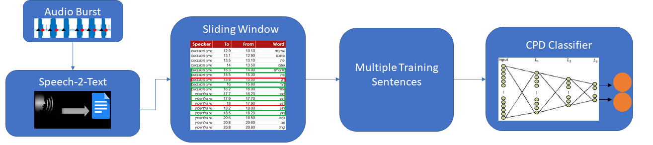
Figure 1: An illustration of the Sliding-Windows method applied over the transformed textual conversations, which were then fed as training samples into a Fully-Connected Neural Network that classified whether a given instance was a CPD or not.

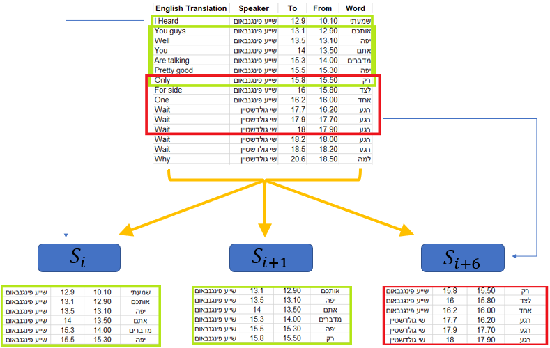
(a) An illustration of the Sliding-Window method applied over a given textual conversation (after the Speech-2-Text transformation), and iterative computation of Sliding-Windows through the continuous text. The red frame ($S_{i+6}$) represents an example of a speaker interchange; i.e., a change point, whereas the green frames ($S_{i},S_{i+1}$) are an example of a non change point examples. The column English Translation stands for translation from Hebrew to English (not in the dataset, used solely for the purposes of this paper). The challenges presented in the Related Work (Section 2) related to Hebrew analysis are listed in this column for each utterance or phrase.

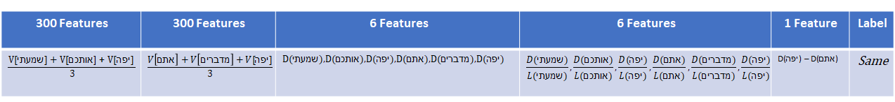
(b) Computation of a concatenated Feature-Vector $V_{i}$ for the Sliding-Window $S_{i}$ presented in Figure 2(a); $V_{i}$ was concatenated by - (i) the vectorial average representation of $S_{i}^{I}$, (ii) the vectorial average representation of $S_{i}^{II}$, (iii) the duration of each of the words in $S_{i}$, i.e. $\{W_{i}^{j}\}_{j=1}^{6}$, denoted by $D(W_{i}^{j})$, (iv) the ratio of the duration of each word in $S_{i}$, and its length in characters (denoted by $L(W_{i}^{j})$), and (v) the time elapsed between $W_{i}^{3}$ and $W_{i}^{4}$ in $S_{i}$. For illustrative purposes, we added the label of $S_{i}$ ($Split$).

Figure 2: Creation of training instances using the Sliding-Window method, and illustration of the feature encoding process. Each column represents the number of cells concatenated to the feature vector.

For each conversation of size $n$, we iterated over all of the $n$ words (see Figure 2(a)) and divided the conversation into tuples of six words, using the sliding window method. This resulted in $n-5$ tuples (windows), denoted as S={$S_{1}$,$S_{2}$,…,$S_{n-5}$}. The first window, $S_{1}$, was composed of the first six words ($W_{1}^{1},W_{1}^{2},..,W_{1}^{6}$). Similarly, $S_{2}$ was composed of the next six word tuple ($W_{2}^{1},W_{2}^{2},\ldots,W_{2}^{6}$) and so on to the last window, $S_{n-5}$ which included ($W_{n-5}^{1},W_{n-5}^{2},\ldots,W_{n-5}^{6}$). For each arbitrary sliding window $S_{i}$ ($1\leq i\leq n-5$), we computed the Word-2-Vec  [39, 38] vectorial average of the first and last three words in the sliding window $S_{i}$, denoted by $S_{i}^{I}=\{W_{i}^{1},W_{i}^{2},W_{i}^{3}\}$ and $S_{i}^{II}=\{W_{i}^{4},W_{i}^{5},W_{i}^{6}\}$, respectively. For the Word-2-Vec based computation, we used the Word-2-Vec pre-trained vectors vocabulary file in Hebrew, published by Facebook (available at Facebook pre-trained Word-2-Vec Models). Since every word in the vocabulary was represented as a multi-dimensional vector of size $300$, this step in the feature engineering process generating 600 features (300 for $S_{i}^{I}$, and 300 for $S_{i}^{II}$. In addition, even though our solution was mainly NLP based, our feature-engineering process generated additional $13$ meta-vocal based features, for each of the six words in $S_{i}$, as follows:

1. Duration of each word in $S_{i}$.

2. Speech rate of each word, represented by the length of a given word (in characters), divided by its duration.

3. Time elapsed between the third word $W_{i}^{3}$, and the fourth word $W_{i}^{4}$ in $S_{i}$, that can intuitively imply about some percentage of confidence in the detection of change point.

Figure 2(b) visualizes the full feature vector of size 613 engineered for each Sliding-Window. Finally, for each window, we added the label for the target feature (i.e., $Same$ or $Split$). If there was a change of speakers between the third and fourth word, this instance was labeled $Split$. Otherwise, the label was $Same$.

4 Classification Using a Fully-Connected Neural Network

Our feature engineering process resulted in 1,129,570 sliding windows instances, which were converted into feature-vector based learning examples. These examples were divided into training and test sets, using the well known Cross-Validation method  [53, 30, 2], such that 80% of the learning examples were used for the training set, and the remaining 20% for test. Due to the tabular structure of the transformed dataset using the Sliding-Window method, the model chosen for the classification problem was a Deep Neural Network with a Fully Connected (DNN-FC) architecture. The Neural Network has three hidden layers, and a dropout layer between any two layers, as well as between the last hidden layer and the output layer, with $p=0.5$ for all the dropout layers (see Table 2 for a specific input size and Neural Network layer dimension, and Figure 3 for an illustration of the Neural Network’s architecture).

Layer	In Features	Out Features
Input	613	307
$1^{st}$ Hidden Layer	307	154
$2^{nd}$ Hidden Layer	154	77
$3^{rd}$ Hidden Layer	77	2
Output	2	Softmax Decision Function

Table 2: Neural Network Architecture

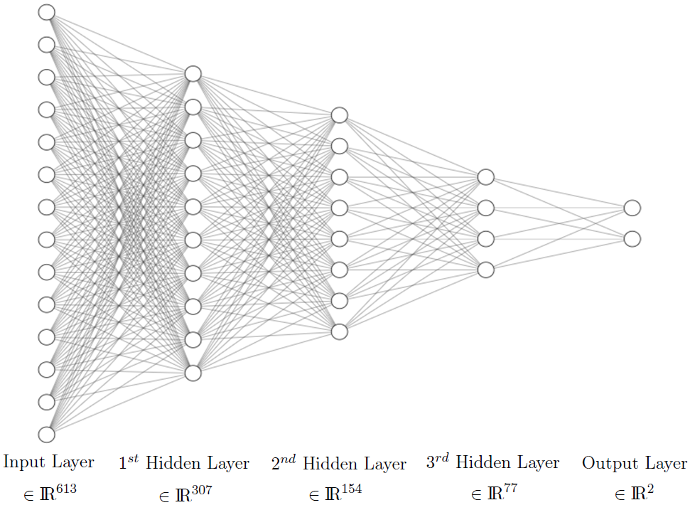
Figure 3: A visual depiction of the Neural Network with a Fully-Connected architecture and the dimensions of each layer (via a web-tool available at the NN-SVG tool). The Neural Network has three hidden layers with a dropout layer between each hidden layer and its following layer, as well as between the Input Layer and the $1^{st}$ Hidden Layer; the dropout layers are only reflected during the Neural Network’s training process, with the probability of $p=0.5$ to remove a random neuron from the Neural Network.

Since our problem is an instance of a supervised classification, we used the Cross-Entropy (CE) loss function  [65]. This loss function measures the performance of a classification model whose output is a probability value between 0 to 1 for each label (i.e. the CE loss increases as the predicted probability diverges from the actual label). As for the learning rate of the Neural Network, we used the Adam Optimizer  [29, 64], an adaptive learning rate method that computes individual learning rates for different parameters, with an initial learning rate value of $\alpha=1\cdot 10^{-4}$. Consequently, we chose a Softmax [45, 46] activation layer to represent the network’s output, in the form of a probability vector of size 2 for the Softmax layer which predicts the probability of an instance being labeled as $Split$ and $Same$, with one probability for each class.

5 Experimental Evaluation

In this section we validate our hypothesis that the classification framework suggested in this paper results in accurate and effective speaker change point detection. Specifically, we show that using NLP techniques for CPD in a multi-speaker environment can outperform classical speech techniques. For this purpose, we used human experts to tag the dataset by assigning a label of speaker identity to each word, in a given audio burst that was converted into a list of words (with the additional features as the start and end times of the word). Clearly, there is no need in a human labeling process for future dataset classification (apart from evaluation purposes), since the TSCPD model aims to detect the change points, rather than speaker identities of each vocal segment. Unlike typical voice-based solutions ([63, 57]) which require the speaker identities, the TSCPD model need to know whether an interchange has occurred or not, independent of the speaker identities before and after the interchange.

The last thing that had to be considered while training the neural network was the ratio of the examples from $Split$ class to the examples from $Same$ class. One could argue that the construction of a classifier which always returns $Same$ as a label would be good, since, this classifier would produce $\sim$ 98% of precision on our dataset. This is due to the fact that in a given natural conversation, the proportion of speech is higher than the number of turns. Thus, this classifier is of limited utility for our purposes to find and identify change points. To do so, our method takes the relative weight of the examples from class $Split$ into account. As mentioned in Section 3, the comparative proportions of the $Split$ and $Same$ classes were 1.5% and 98.5% respectively. Thus, when defining the loss function of the neural network, we defined the weight of each class to be the inverse of the number of examples from this class, i.e. $\frac{1}{|Split|}$ for class $Split$, and $\frac{1}{|Same|}$ for class $Same$ (where $|Split|$ and $|Same|$ represent the number of examples from each class).

The remainder of this section presents the evaluation process as follows:

• Section 5.1 analyze the robustness of TSCPD model to a variable number of speakers, compared to the voice based diarization solutions presented in [63, 57].

• Section 5.2 analyze the robustness of TSCPD model to a completely new speakers that were not seen during the training process.

• Section 5.3 compares the TSCPD model to a Deep Learning approach - an Auto Encoder, and Machine Learning algorithms, such as XG-Boost, SVM, Decision-Tree and k-NN.

• Section 5.4 analyze the robustness of TSCPD model to a different source of Speech-2-Text engine.

5.1 The Number of Speakers Influences Model Efficiency

The objective of this work was to tackle the CPD problem mainly in terms of its dependence on the number of speakers, which is a key issue when attempting to solve the SD\SV problems with voice based solutions. The work presented in [63] utilized the speech embedding extraction module in [57], by learning the extracted speaker-discriminative embeddings, or D-vectors, from input utterances. In order to show our model’s robustness to the number of speakers, and compare our work to the speech embedding extraction module, we translated the SD problem into a CPD. For this purpose, we compared our model and the one presented in [63], with a variable number of speakers $k\in\{8,20,50,100,200,250,500,1000\}$, and with 10 different random speakers sampling’s identities and utterances, using the following procedure:

1. Step one consisted of splitting our dataset into a textual speaker utterances. Since each word duration is known (by substracting the "to" from the "from" columns), as well as the speaker identity, we could retrieve a textual speaker utterance for each one in the dataset.

2. Step 2 consisted of segmenting each audio file according to its timeline speaker utterances. Then, we trained the neural network presented in [57], to extract the speech embedding vectors for each speaker utterance, i.e. the D-vectors.

3. The D-vectors extracted for each speaker utterance formed a matrix of size $N_{seg}\times M_{emb}$, where $N_{seg}$ represents the number of segments extracted for each speaker utterance, and $M_{emb}$ is the D-vector which $\in\rm I\!R^{256}$. The segments for each speaker utterance were extracted using a Voice Activity Detector (VAD) engine, using the $webrtcvad$ and $librosa$ Python libraries.

4. Then, we split our converted to speech utterances dataset; i.e., the speech embedding matrices for each speaker utterance, into training and test sets with a 80%-20% division of the data samples respectively. Clearly, the number of data samples for each speaker identity out of the total of 1,240 was assigned proportionally to the training and test sets.

5. The work in [63] presents a fully-supervised speaker diarization model termed UIS-RNN, and assigns a speaker identity to each speaker utterance in the dataset. As such, we trained the UIS-RNN presented in [63], by the training matrices, each of which represented a set of D-vectors extracted as function of the number of segments in each speaker utterance.

For each number of speakers $k\in\{8,20,50,100,200,250,500,1000\}$, we ran this procedure 10 times, each time with a randomly chosen set of speakers. In order to calculate the error rate of each result for each number of $k$, we converted the model’s inference results into CPD based results, i.e. a binary classification testing. For each speaker utterance in the test set, the UIS-RNN model produced a classification vector of size $N_{seg}$. Hence, we could conduct Type I, Type II  [4] errors analyses for each classification vector, which later resulted in Precision, Recall and F1-Score calculations. For a given conversation split into $U\in\mathbb{N}$ speaker utterances, the Type I and Type II errors analysis was as follows:

• Type I - occurs any time when in a given speaker utterance $u_{i}$ (for $1\leq i\leq|U|$), the first segment label in its corresponding classification vector had different values than each of the classification vector elements. More specifically, for a classification vector $c_{i}$ (that represents the identity assignments for $u_{i}$ segments) of size $\ell$, we count an error each time $c_{i}[j]$ is not equal to $c_{i}[1]$ for $2\leq j\leq\ell$. Each such mismatch implies that the UIS-RNN detected a change point and tagged $"Split"$, rather than $Same$.

• Type II - occurs any time when the last segment of a speaker utterance $u_{i}$ classification, and the first segment of $u_{i+1}$ classification are equal (for $1\leq i\leq|U|-1$). This is due to the fact that between any proceedings $u_{i}$ and $u_{i+1}$ there must have been an interchange, i.e. the UIS-RNN tagged $Same$, rather than $Split$.

Random Model List - TSCPD, UIS-RNN
Speakers	TSCPD Precision    Recall     F1-Score	UIS-RNN Precision   Recall     F1-Score
8	96.56(1.03)  95.11(0.94)  95.78(0.85)	95.94(1.11) 97.74(0.93)  96.65(1.36)
20	96.34(1.87)  94.43(3.36)  95.30(2.55)	94.87(2.53) 96.67(1.82)  95.15(2.75)
50	96.54(0.55)  91.21(2.34)  93.55(1.51)	94.56(1.75) 96.60(0.92)  94.98(1.34)
100	96.90(0.45)  87.42(1.50)  91.50(0.88)	94.26(1.17) 95.83(0.63)  95.03(1.00)
200	97.09(0.22)  84.50(2.22)  89.79(1.41)	94.48(1.42) 92.14(0.87)  93.29(1.32)
250	97.03(0.20) 83.72(1.16) 89.30(0.79)	95.84(0.32) 82.05(0.55)  87.76(0.25)
500	97.17(0.13) 83.44(1.56) 89.15(0.94)	96.05(0.62) 79.40(1.13)  86.18(0.63)
1000	97.13(0.16) 82.77(0.95) 88.71(0.60)	96.04(0.39) 79.21(1.16)  86.04(0.70)
1240	97.19(0.00) 82.12(0.00) 89.02(0.00)	95.72(0.00) 79.37(0.00)  86.78(0.00)

Table 3: Results table for the randomly chosen speaker process, a comparison of our model versus Google’s D-vector based model. For each number of speakers $k\in\{8,20,50,100,200,250,500,1000\}$ the average values of the Precision, Recall and F1-Score are presented for 10 different data samplings. For 1,240 speakers we ran the process only once, for purposes of a full comparison (TSCPD and UIS-RNN models). The Standard-Deviation $\sigma$ appears in parentheses.

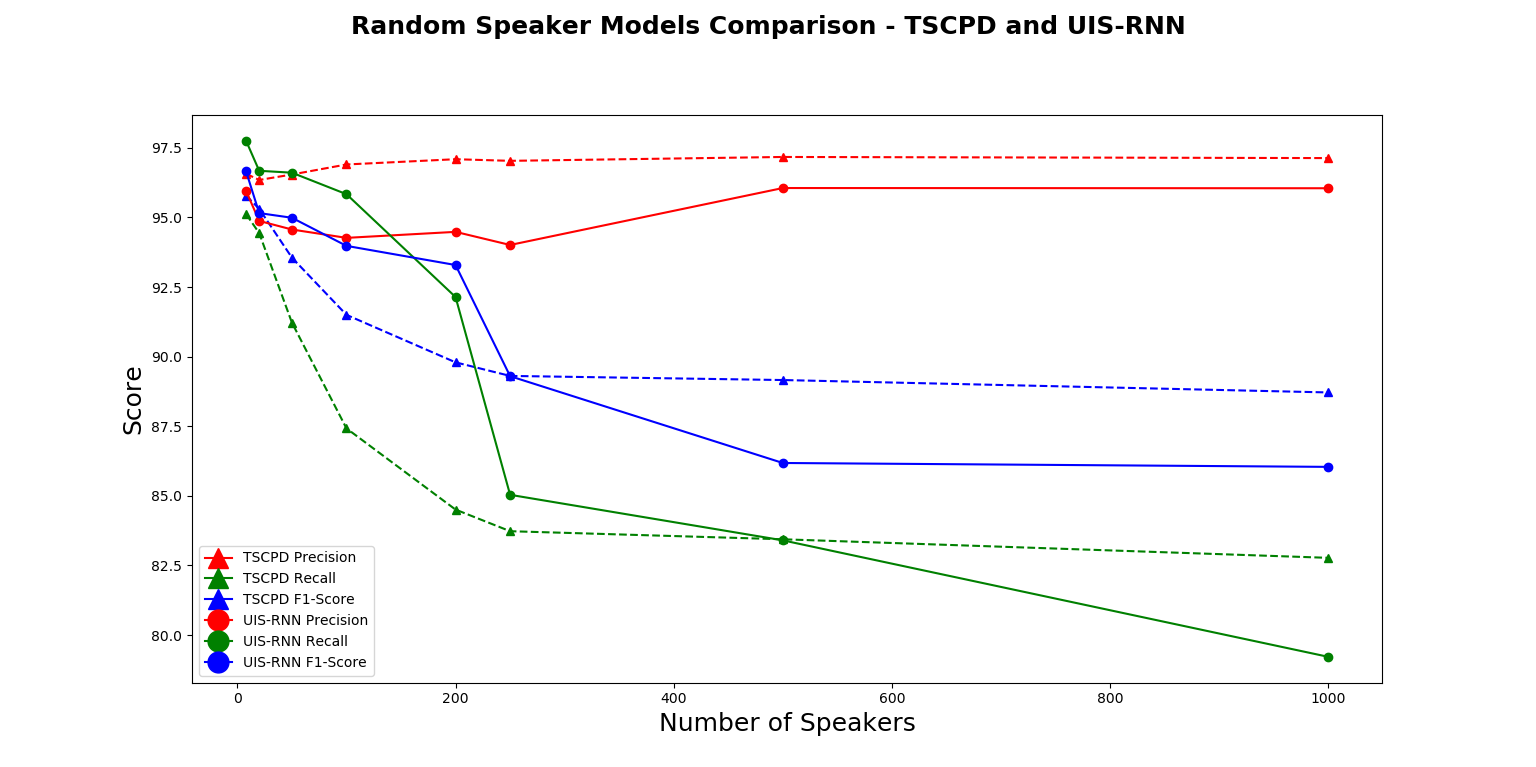
Figure 4: Graphical results for the comparison process performed as explained in Sub-Section 5.1. As shown, the Recall and F1-Score drop dramatically when using the UIS-RNN model, whenever that there is an increase in the number of speakers in the dataset.

The results for this comparison are presented in Table 3, and a graphical illustration of the performance for the TSCPD and UIS-RNN models are presented in Figure 4. In addition, as can be seen in Table 3, we compared the models with the whole dataset, i.e. with all of the 1,240 speakers. For this purpose, we ran the described above procedure only once randomly. It is clear that from 250 speakers and up, the TSCPD model outperform the UIS-RNN model in $all$ measurements. Both of the models maintained their Precision due to the extreme class imbalance, but as the number of speakers in the dataset increased - the TSCPD model outperformed the UIS-RNN. The UIS-RNN model’s Recall (and as such the F1-Score) deteriorated, since there were many more speaker identities to classify, whereas the TSCPD remained quite robust to the increase in number of speakers in the dataset.

The Precision and Recall measures (and as such the F1-Score) and Type I & II errors are very closely related since they are both defined by terms such as true/false positive, and true/false negative. Due to the intuitive and clear numerical representation of the Precision, Recall and F1-Score measurements, we have chosen to report the results by this terms, rather than Type I and Type II errors.

Figure 5 presents the Confusion Matrix as well as a graphical illustration of the Receiver Operating Characteristic (ROC). Its corresponding Area Under Curve (AUC) appears in Figure 6 for the performance of the TSCPD model for the 1,240 speaker based dataset. The graphs presented in Figure 6, suggest the following:

• As the False Positive value declines, the better the model predicts examples of the $Same$ class with high probability, and vice versa for the True Positive value that correspond to the $Split$ class.

• The TSCPD model is quite robust despite the class imbalance, a fact which is reflected in the superiority of the micro-average ROC curve as well as its area under curve as compared to the macro-average ROC curve (and its area under curve). The robustness is manifested in this superiority, since the macro-average independently computes the metric for each class, and then takes the average result (hence treating all classes equally), whereas a micro-average aggregates the contributions of all classes to compute the average metric.

  

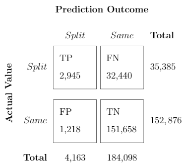
  Figure 5: Confusion Matrix results achieved by the TSCPD model for 1,240 speakers. We treat the $Split$ as the positive class, and vice versa for $Same$. Note the high precision for both classes, even though the positive class barely represents 1.5% of the dataset examples.

  

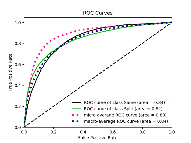
  Figure 6: ROC curves for the TSCPD model performance for 1,240 speakers, as well as the AUC for each curve (see Legend). The black and green curves represent the True Positive Rate as a function of the False Positive Rate for the $Same$ and $Split$ classes respectively. The dashed blue and pink curves represent the same relationship for the computation of micro and macro averages.

5.2 Model Robustness to Unseen Speakers

Next, we show the robustness and strength of our context based TSCPD model to speakers that were not included in the train set. This means testing whether the TSCPD model is robust to new speakers with (potentially) new different speech rate, that were not used in training the Neural Network. We call this model Textual Speaker Change Point Detection - for Unseen Speakers (TSCPD-US). For this purpose, we have split our dataset into training and test sets, by randomly accumulating CSV files (representing transformed Speech-2-Text conversations) up to $k\in\{100,200,500,1000\}$ unseen-during-training-time speakers for the test set, and the rest of the CSV files containing $1,240-k$ speakers for the training set. This ensured that the Neural Network would be only trained on a subset of speakers that were not part of the conversations that served for the test set. Similar to the procedure described in Section 5.1, for each value of $k$ we ran this dataset splitting 10 times, each time with randomly sampled speakers. The calculation of the average score for each of the 10 random samplings (for each $k$ value), we showed that performance was comparable (with respect to the TSCPD model) when inserting new unseen speakers in the test process. The results for this section are presented in Table 4, which depicts the slight degradation whenever we insert new unseen speakers to the CPD system. This is graphically illustrated in Figure 7. These results suggest that whenever $k\geq 200$ completely new unseen tested speakers, the TSCPD converges to robustness around the F1-Score.

Random Models List - TSCPD, TSCPD-US
Speakers in Test	TSCPD Precision   Recall   F1-Score	TSCPD-US Precision   Recall   F1-Score
100	96.90(0.45) 87.42(1.50) 91.50(0.88)	97.22(0.23) 83.55(1.22) 89.86(0.63)
200	97.09(0.22) 84.50(2.22) 89.79(1.41)	96.68(0.52) 82.54(0.71) 89.06(0.47)
500	97.17(0.13) 83.44(1.56) 89.15(0.94)	96.48(1.02) 82.62(1.31) 89.01(1.15)
1000	97.13(0.16) 82.77(0.95) 88.71(0.60)	96.75(0.49) 82.03(0.53) 88.78(0.31)

Table 4: Results for the randomly chosen speakers process, comparing the TSCPD and TSCPD models, that tested on a random unseen number of speakers $k\in\{100,200,500,1000\}$. The Standard-Deviation $\sigma$ appears in parentheses.

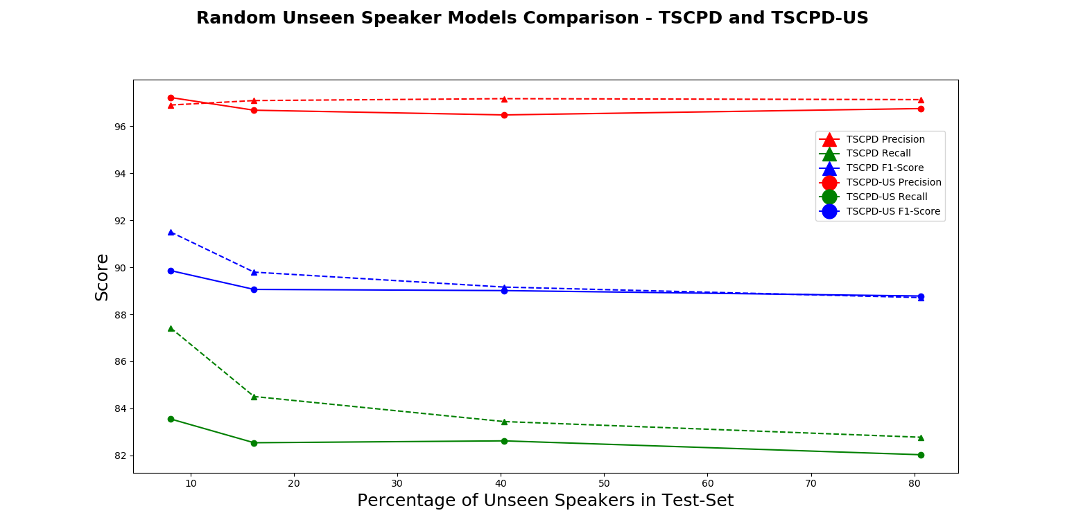
Figure 7: Graphical illustration of the comparison the TSCPD and TSCPD-US models, as described in Sub-Section 5.2. The X-axis represents the percentage of speakers on whom the TSCPD model was not trained on, i.e. the percentage of new speakers that were introduced to the system. The Y-axis represents the score for Precision, Recall, and the F1-Score. Note the robustness of the TSCPD and TSCPD-US in the plot.

5.3 Classical Machine and Deep Learning Models

Here, we present the comparison to several Deep and Machine Learning models. Specifically, we used the well known Auto Encoder model [5, 33], since Auto Encoders tend to be applied for Anomaly Detection problems (like the CPD). Using Auto Encoders to detect anomalies usually involves two main steps:

1. First, we feed our dataset into an Auto Encoder and tune it until it is well trained to reconstruct the expected output with minimum error. An Auto Encoder is well-trained if the reconstructed output is sufficiently close to the input and if the Auto Encoder is able to successfully reconstruct most of the data this way.

2. Then, we feed all our dataset again to our trained Auto Encoder and measure the error term of each reconstructed data point. In other words, we measure how far the reconstructed data point is from the actual data-point. A well-trained Auto Encoder essentially learns how to reconstruct an input that follows a certain format, so if we provide a badly formatted data point to a well-trained Auto Encoder, we are likely to get something quite different from our input and a large error term.

The Encoder and Decoder parts of the Auto Encoder that we built for this comparison were based on the architecture we used in our Fully-Connected Neural Network, without the $3^{rd}$ hidden and output layers (see Table 2). In other words, the Encoder was reduced from an input layer size to a $2^{nd}$ hidden layer size, then expanded into the Decoder through the context vector, i.e. from the $2^{nd}$ hidden layer size to the input layer size. However, the Auto Encoder model failed to outperform the TSCPD model.
In addition, we examined well-known Machine Learning algorithms to determine whether we could achieve better results than the ones reported in the previous sub-sections. We examined the XGBoost, Support Vector Machine (SVM), Decision-Tree, and $k-NN$ where $k\in\{1,3,5,7,9\}$. As can be seen in Table 5, neither Auto-Encoder approach, nor traditional Machine Learning algorithms outperformed the TSCPD model.

For the different values of $k$ for the k-NN models, Figure 8 presents the $k-NN$ results graph that sums up the Precision, Recall and F1-Score achieved by using the $k-NN$ algorithm. It is easy to see that the TSCPD model outperformed each of the classical models in terms of Precision and F1-Score, but only achieved lower Recall values in some of the cases (SVM, 5-NN, 9-NN).

Machine & Deep Learning Models Results Table
Model / Indicator	Precision	Recall	F1-Score
TSCPD	97.19 %	82.12 %	89.02 %
Auto Encoder	96.81 %	78.16 %	85.85 %
XGBoost	74.27 %	81.28 %	77.62 %
SVM	74.04 %	83.26 %	78.38 %
Decision-Tree	75.18 %	74.80 %	74.99 %
1-NN	75.03 %	75.23 %	75.13 %
3-NN	74.74 %	78.56 %	76.60 %
5-NN	74.75 %	82.83 %	78.58 %
7-NN	74.57 %	81.39 %	77.83 %
9-NN	74.45 %	83.14 %	78.55 %

Table 5: Results of the comparison between the TSCPD model and the classical Deep and Machine Learning approaches - the Auto Encoder model for the Deep Learning approach, and XG-Boost, SVM, Decision-Tree and $k$-NN for the Machine Learning algorithms.

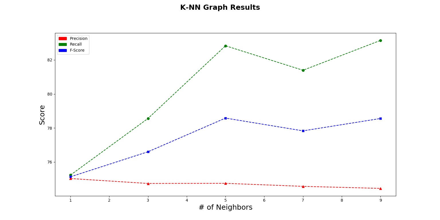
Figure 8: Precision, Recall and F1-Score for $k$-NN model over the dataset, when $k\in\{1,3,5,7,9\}$. As reported in sections  5.1, 5.2 and 5.3, the TSCPD achieved 97.19% for Precision, 82.12% for Recall, and 89.02% for the F1-Score.

5.4 New Speech-2-Text Data

In Section 3, we described the 1,692 vocal conversations that went through the transformation into the text process using a commercial Speech-2-Text engine. In order to further confirm the robustness of the TSCPD model to a new Speech-2-Text engine , we collected an additional 362 vocal conversations with 431 new speakers from similar TV shows and radio programs in Israel, as in our original dataset. These 362 conversations with 431 new speakers were converted using Google’s corpora Speech-2-Text engine, and then transformed into a continuous text, in the same manner as for our initial dataset. Then, we trained and tested the TSCPD model the same way as we did for our initial dataset.

The comparison between our dataset and the new Speech-2-Text dataset is presented in Table 6. It shows that the disparity between the TSCPD model and its performance over the new Speech-2-Text engine manifested mainly in the Recall measurement, and as such over the F1-Score as well. Even though the TSCPD model performance was degraded, it still demonstrated its robustness to a new Speech-2-Text engine.

Results for the Google Speech-2-Text Data
Model / Indicator	Precision	Recall	F1-Score
TSCPD	97.19 %	82.12 %	89.02 %
TSCPD for Google Speech-2-Text Engine	96.82 %	76.47 %	85.45 %

Table 6: Comparison of the results for the TSCPD model trained on 1,240 speakers, to the results for the TSCPD model applied to a new dataset with 431 different speakers, transformed using the Google Speech-2-Text engine.

6 Conclusions and Future Work

In this paper we demonstrated how to solve the CPD variant of the SD problem, and focused on the number of speakers and the conversational context using an intelligent NLP based technique. We showed that we can achieve better results and greater robustness compared to two recently developed voice based solutions to the SD\SV problems, and found that our model outperforms other classical Machine and Deep Learning approaches. Even though obtaining better results, the SD problem is still not completely solved. Hence, one possible future research direction would be to address the SD problem with NLP techniques; i.e., to move from the CPD problem towards the full SD problem, including an NLP based assignment to the speaker utterances module. Another possible future work direction would involve addressing the CPD or the SD problems, multi-lingually by solving each problem for many languages by training a cross-lingual model.

7 Acknowledgment

This work was supported by the Ariel Cyber Innovation Center in conjunction with the Israel National Cyber directorate in the Prime Minister’s Office. In addition, we wish to thank to IFAT Group that provided the dataset for this research, as well as the human labeling process for the speaker identities, and express our gratitude to the Israel Innovation Authority (IIA) for funding this study.

References

- [1] A. Ahmed and E. Xing. Dynamic non-parametric mixture models and the recurrent chinese restaurant process: with applications to evolutionary clustering. In Proceedings of the 2008 SIAM International Conference on Data Mining, pages 219–230. SIAM, 2008.
- [2] S. Arlot, A. Celisse, et al. A survey of cross-validation procedures for model selection. Statistics surveys, 4:40–79, 2010.
- [3] P. Balamurugan. A survey on speaker diarization approach for audio and video content retrieval.
- [4] A. Banerjee, U. Chitnis, S. Jadhav, J. Bhawalkar, and S. Chaudhury. Hypothesis testing, type i and type ii errors. Industrial psychiatry journal, 18(2):127, 2009.
- [5] D. Berthelot, C. Raffel, A. Roy, and I. Goodfellow. Understanding and improving interpolation in autoencoders via an adversarial regularizer. arXiv preprint arXiv:1807.07543, 2018.
- [6] D. M. Blei and P. I. Frazier. Distance dependent chinese restaurant processes. Journal of Machine Learning Research, 12(Aug):2461–2488, 2011.
- [7] A. Brendel, B. Laufer-Goldshtein, S. Gannot, R. Talmon, and W. Kellermann. Localization of an unknown number of speakers in adverse acoustic conditions using reliability information and diarization. In ICASSP 2019-2019 IEEE International Conference on Acoustics, Speech and Signal Processing (ICASSP), pages 7898–7902. IEEE, 2019.
- [8] F. Camci. Change point detection in time series data using support vectors. International Journal of Pattern Recognition and Artificial Intelligence, 24(01):73–95, 2010.
- [9] R. Chalapathy and S. Chawla. Deep learning for anomaly detection: A survey. arXiv preprint arXiv:1901.03407, 2019.
- [10] R. K. Chatterjee and A. Kar. Optimal global threshold estimation using statistical change-point detection. Signal & Image Processing: An International Journal (SIPIJ), 8(4), 2017.
- [11] P. Cyrta, T. Trzciński, and W. Stokowiec. Speaker diarization using deep recurrent convolutional neural networks for speaker embeddings. In International Conference on Information Systems Architecture and Technology, pages 107–117. Springer, 2017.
- [12] A. Das, U. Bhattacharjee, and D. K. Mitra. One-decade survey on speaker diarization for telephone and meeting speech. 2017.
- [13] D. Dimitriadis and P. Fousek. Developing on-line speaker diarization system. In INTERSPEECH, pages 2739–2743, 2017.
- [14] P. Dokas, L. Ertoz, V. Kumar, A. Lazarevic, J. Srivastava, and P.-N. Tan. Data mining for network intrusion detection. In Proc. NSF Workshop on Next Generation Data Mining, pages 21–30, 2002.
- [15] E. El-Khoury, C. Senac, and J. Pinquier. Improved speaker diarization system for meetings. In 2009 IEEE International Conference on Acoustics, Speech and Signal Processing, pages 4097–4100. IEEE, 2009.
- [16] E. Fini and A. Brutti. Supervised online diarization with sample mean loss for multi-domain data. arXiv preprint arXiv:1911.01266, 2019.
- [17] Y. Goldberg and M. Elhadad. Word segmentation, unknown-word resolution, and morphological agreement in a hebrew parsing system. Computational Linguistics, 39(1):121–160, 2013.
- [18] Z. Harchaoui, F. Vallet, A. Lung-Yut-Fong, and O. Cappé. A regularized kernel-based approach to unsupervised audio segmentation. In 2009 IEEE International Conference on Acoustics, Speech and Signal Processing, pages 1665–1668. IEEE, 2009.
- [19] C. Hartland, N. Baskiotis, S. Gelly, M. Sebag, and O. Teytaud. Change point detection and meta-bandits for online learning in dynamic environments. 2007.
- [20] G. Heigold, I. Moreno, S. Bengio, and N. Shazeer. End-to-end text-dependent speaker verification. In 2016 IEEE International Conference on Acoustics, Speech and Signal Processing (ICASSP), pages 5115–5119. IEEE, 2016.
- [21] I. Himawan, M. H. Rahman, S. Sridharan, C. Fookes, and A. Kanagasundaram. Investigating deep neural networks for speaker diarization in the dihard challenge. In 2018 IEEE Spoken Language Technology Workshop (SLT), pages 1029–1035. IEEE, 2018.
- [22] S. Hochreiter and J. Schmidhuber. Long short-term memory. Neural computation, 9(8):1735–1780, 1997.
- [23] M. Hrúz and Z. Zajíc. Convolutional neural network for speaker change detection in telephone speaker diarization system. In 2017 IEEE International Conference on Acoustics, Speech and Signal Processing (ICASSP), pages 4945–4949. IEEE, 2017.
- [24] M. À. India Massana, J. A. Rodríguez Fonollosa, and F. J. Hernando Pericás. Lstm neural network-based speaker segmentation using acoustic and language modelling. In INTERSPEECH 2017: 20-24 August 2017: Stockholm, pages 2834–2838. International Speech Communication Association (ISCA), 2017.
- [25] Y. Intrator, G. Katz, and A. Shabtai. Mdgan: Boosting anomaly detection usingmulti-discriminator generative adversarial networks. arXiv preprint arXiv:1810.05221, 2018.
- [26] J. Jung, H. Heo, I. Yang, S. Yoon, H. Shim, and H. Yu. D-vector based speaker verification system using raw waveform cnn. In 2017 International Seminar on Artificial Intelligence, Networking and Information Technology (ANIT 2017). Atlantis Press, 2017.
- [27] P. Kenny, D. Reynolds, and F. Castaldo. Diarization of telephone conversations using factor analysis. IEEE Journal of Selected Topics in Signal Processing, 4(6):1059–1070, 2010.
- [28] T. Kieu, B. Yang, and C. S. Jensen. Outlier detection for multidimensional time series using deep neural networks. In 2018 19th IEEE International Conference on Mobile Data Management (MDM), pages 125–134. IEEE, 2018.
- [29] D. P. Kingma and J. Ba. Adam: A method for stochastic optimization. arXiv preprint arXiv:1412.6980, 2014.
- [30] R. Kohavi et al. A study of cross-validation and bootstrap for accuracy estimation and model selection. In Ijcai, volume 14, pages 1137–1145. Montreal, Canada, 1995.
- [31] B. Laufer-Goldshtein, R. Talmon, and S. Gannot. Diarization and separation based on a data-driven simplex. In 2018 26th European Signal Processing Conference (EUSIPCO), pages 842–846. IEEE, 2018.
- [32] M. Lavielle and G. Teyssiere. Adaptive detection of multiple change-points in asset price volatility. In Long memory in economics, pages 129–156. Springer, 2007.
- [33] X. Li, Z. Chen, L. K. Poon, and N. L. Zhang. Learning latent superstructures in variational autoencoders for deep multidimensional clustering. arXiv preprint arXiv:1803.05206, 2018.
- [34] Q. Lin, R. Yin, M. Li, H. Bredin, and C. Barras. Lstm based similarity measurement with spectral clustering for speaker diarization. arXiv preprint arXiv:1907.10393, 2019.
- [35] C. Luo, X. Wu, T. F. Zheng, and L. Wang. Segmentation-based method for text-dependent speaker recognition in embedded applications. Asia-Pacific Signal and Information Processing Association, APSIPA ASC, 2010.
- [36] P. A. Mansfield, Q. Wang, C. Downey, L. Wan, and I. L. Moreno. Links: A high-dimensional online clustering method. arXiv preprint arXiv:1801.10123, 2018.
- [37] Z. Meng, L. Mou, and Z. Jin. Hierarchical rnn with static sentence-level attention for text-based speaker change detection. In Proceedings of the 2017 ACM on Conference on Information and Knowledge Management, pages 2203–2206, 2017.
- [38] T. Mikolov, K. Chen, G. Corrado, and J. Dean. Efficient estimation of word representations in vector space. arXiv preprint arXiv:1301.3781, 2013.
- [39] T. Mikolov, I. Sutskever, K. Chen, G. S. Corrado, and J. Dean. Distributed representations of words and phrases and their compositionality. In Advances in neural information processing systems, pages 3111–3119, 2013.
- [40] A. More and R. Tsarfaty. Data-driven morphological analysis and disambiguation for morphologically rich languages and universal dependencies. In Proceedings of COLING 2016, the 26th International Conference on Computational Linguistics: Technical Papers, pages 337–348, 2016.
- [41] M. Nicolau, J. McDermott, et al. A hybrid autoencoder and density estimation model for anomaly detection. In International Conference on Parallel Problem Solving from Nature, pages 717–726. Springer, 2016.
- [42] E. Page. A test for a change in a parameter occurring at an unknown point. Biometrika, 42(3/4):523–527, 1955.
- [43] E. S. Page. Continuous inspection schemes. Biometrika, 41(1/2):100–115, 1954.
- [44] J. Pardo, X. Anguera, and C. Wooters. Speaker diarization for multiple-distant-microphone meetings using several sources of information. IEEE Transactions on Computers, 56(9):1212–1224, 2007.
- [45] Z. Qin and D. Kim. Rethinking softmax with cross-entropy: Neural network classifier as mutual information estimator. arXiv preprint arXiv:1911.10688, 2019.
- [46] Z. Qin and D. Kim. Softmax is not an artificial trick: An information-theoretic view of softmax in neural networks. arXiv preprint arXiv:1910.02629, 2019.
- [47] D. A. Reynolds and P. Torres-Carrasquillo. The mit lincoln laboratory rt-04f diarization systems: Applications to broadcast audio and telephone conversations. Technical report, MASSACHUSETTS INST OF TECH LEXINGTON LINCOLN LAB, 2004.
- [48] E. Schubert, A. Zimek, and H.-P. Kriegel. Local outlier detection reconsidered: a generalized view on locality with applications to spatial, video, and network outlier detection. Data Mining and Knowledge Discovery, 28(1):190–237, 2014.
- [49] D. Seddah, R. Tsarfaty, S. Kübler, M. Candito, J. Choi, R. Farkas, J. Foster, I. Goenaga, K. Gojenola, Y. Goldberg, et al. Overview of the spmrl 2013 shared task: cross-framework evaluation of parsing morphologically rich languages. Association for Computational Linguistics, 2013.
- [50] G. Sell and D. Garcia-Romero. Speaker diarization with plda i-vector scoring and unsupervised calibration. In 2014 IEEE Spoken Language Technology Workshop (SLT), pages 413–417. IEEE, 2014.
- [51] S. H. Shum, N. Dehak, R. Dehak, and J. R. Glass. Unsupervised methods for speaker diarization: An integrated and iterative approach. IEEE Transactions on Audio, Speech, and Language Processing, 21(10):2015–2028, 2013.
- [52] G. Soldi, C. Beaugeant, and N. Evans. Adaptive and online speaker diarization for meeting data. In 2015 23rd European Signal Processing Conference (EUSIPCO), pages 2112–2116. IEEE, 2015.
- [53] M. Stone. Cross-validatory choice and assessment of statistical predictions. Journal of the Royal Statistical Society: Series B (Methodological), 36(2):111–133, 1974.
- [54] C. Sunitha and E. Chandra. Speaker recognition using mfcc and improved weighted vector quantization algorithm. Int J Eng Technol (IJET), 7(5):1685–1692, 2015.
- [55] C. Truong, L. Oudre, and N. Vayatis. Selective review of offline change point detection methods. Signal Processing, page 107299, 2019.
- [56] J.-P. Vert and K. Bleakley. Fast detection of multiple change-points shared by many signals using group lars. In Advances in neural information processing systems, pages 2343–2351, 2010.
- [57] L. Wan, Q. Wang, A. Papir, and I. L. Moreno. Generalized end-to-end loss for speaker verification. In 2018 IEEE International Conference on Acoustics, Speech and Signal Processing (ICASSP), pages 4879–4883. IEEE, 2018.
- [58] Q. Wang, C. Downey, L. Wan, P. A. Mansfield, and I. L. Moreno. Speaker diarization with lstm. In 2018 IEEE International Conference on Acoustics, Speech and Signal Processing (ICASSP), pages 5239–5243. IEEE, 2018.
- [59] Q. Wang, H. Muckenhirn, K. Wilson, P. Sridhar, Z. Wu, J. Hershey, R. A. Saurous, R. J. Weiss, Y. Jia, and I. L. Moreno. Voicefilter: Targeted voice separation by speaker-conditioned spectrogram masking. arXiv preprint arXiv:1810.04826, 2018.
- [60] S. H. Yella and H. Bourlard. Overlapping speech detection using long-term conversational features for speaker diarization in meeting room conversations. IEEE/ACM Transactions on Audio, Speech, and Language Processing, 22(12):1688–1700, 2014.
- [61] Z. Zajíc, M. Hrúz, and L. Müller. Speaker diarization using convolutional neural network for statistics accumulation refinement. In INTERSPEECH, pages 3562–3566, 2017.
- [62] Z. Zajíc, D. Soutner, M. Hrúz, L. Müller, and V. Radová. Recurrent neural network based speaker change detection from text transcription applied in telephone speaker diarization system. In International Conference on Text, Speech, and Dialogue, pages 342–350. Springer, 2018.
- [63] A. Zhang, Q. Wang, Z. Zhu, J. Paisley, and C. Wang. Fully supervised speaker diarization. In ICASSP 2019-2019 IEEE International Conference on Acoustics, Speech and Signal Processing (ICASSP), pages 6301–6305. IEEE, 2019.
- [64] Z. Zhang, L. Ma, Z. Li, and C. Wu. Normalized direction-preserving adam. arXiv preprint arXiv:1709.04546, 2017.
- [65] Z. Zhang and M. Sabuncu. Generalized cross entropy loss for training deep neural networks with noisy labels. In Advances in neural information processing systems, pages 8778–8788, 2018.