Emergent gravity from patterns in natural numbers

Abstract

There is natural association of entropy with gravitational systems on one hand and partition of natural numbers on the other hand. We show that given a partition of natural numbers, it is possible to directly associate a metric with it. Gravity emerges from patterns in partition. In the process, metric and matter is unified into a fundamental notion of partition. More precisely, we find a common origin of Schwarzschild metric on one hand and black-hole entropy on the other hand. It immediately implies that information and metric are one and the same and any change in information is stored as change in metric. Thus gravitational radiation carries black-hole entropy worth of information. There are three novel experimental predictions. First, we can retrieve information from the gravitational radiation emitted during merger. Second, if radiation with right information is sent in, black hole absorbs information and decays instead of increasing in mass. This is reverse process of black hole formation. Third, till now only known way of observing nature is through radiation and fields measured far from the source. There is a completely new way of seeing nature if we can capture the whole partition of the source in one go.

1 Motivation

Emergent gravity means two things in this work. First it means equations of gravity are emergent. It is more useful to call this emergent causality as defined below. Second it means metric and matter emerge from some fundamental degrees of freedom. In other words, unification of metric and matter. There are other attempts at emergent gravity for example using Bose-Einstein condensates (Jannes, 2009; Finazzi et al., 2012), entropic gravity (Vancea and Santos, 2012; Verlinde, 2011, 2017), non-commutative geometry (Yang, 2008; Rivelles, 2011), quantum computation (Lloyd, 2005), matrix models (Steinacker, 2010), holographic models (Almheiri et al., 2015; Harlow, 2017; Horowitz and Polchinski, 2006; Kovtun et al., 2005) and many other models (Heckman and Verlinde, 2011; Carlip, 2014; Marolf, 2015). This work is different from all other models as this is the first example of emergent causality.

Causality ensures that events on one time-slice is completely determined by events on another time-slice. At the heart of causality lies differential equations which relate data on two slices. So by causality we mean a system described by differential equation. This is much weaker than lightcone causality. There are at least two handicaps with causality. One it requires choice of initial and boundary condition from outside (Giddings and Strominger, 1988; Hartle and Hawking, 1983; Hartle, 1986; Wudka, 1987). Second, space of theory where differential equations live is separate and independent from the phase space. Space of theory reads coordinates of phase space as input, processes them and returns new coordinates to the phase space. As a result, it requires storing, processing and carrying forward information from one slice to another. For example, be it a classical trajectory or some quantum process, for all practical purposes we work with finite precision. But how does nature process and keep track of large (infinite) number of decimal places? Not only that but also the processes (eg. Feynman diagrams) are infinitely numerous. In quantum gravity it is expected that information is not just a label, but is one and the same as spacetime. Above problem boils down to how information encoded in numbers (input and output of theory) appear as physical space and time (phase space)? We see spacetime and not numbers. Independence means that phase space does not restrict the space of theory. For example, there could have been other consistent gravity, like higher curvature gravity describing our spacetime. It is difficult to argue whether these handicaps are problem or not but it appears to be inefficient.

Weaker definition of causality results in stronger definition of its complement. By emergent causality we mean a system which is not governed by differential equation. Patterns emerge only over some scale. One classic example is distribution of primes. Given $n^{th}$ prime, there is no formula which land us exactly on the next prime but there are formulas which take us close to the next prime. So pattern is emergent. $n^{th}$ prime has some but not all information about other primes. However the system is deterministic as one can list all the primes using the definition. Such a system is free from both the handicap. There is no choice in the initial condition. For example, the first prime is built into the definition of the primes. Second, emergent pattern in density of primes is also invisibly built into the definition of primes. Space of theory is integrated into the phase space.

Equations of motions in physics relate field to its source. Einstein’s equations relate metric to energy-momentum tensor. However it is still a step away from unification because energy-momentum tensor and metric have independent definition. A system having emergent causality is not governed by equations of motion. Thus such a system must relate metric and stress-tensor in a more fundamental way. Presumably metric and matter will be unified into one quantity which can be interpreted either way depending on the way we see it. We will call this emergent matter and emergent spacetime. There is another intuitive way to see this. If fundamentally matter is nothing but information associated with its blackhole entropy. Then spacetime and information must be one and the same in quantum gravity implies that metric and matter must be unified. Things will become clearer as we proceed.

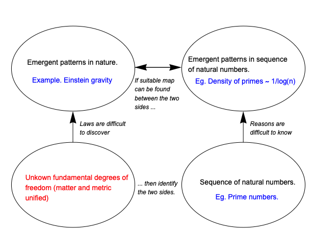
In physics, main source of difficulty lies in handling interaction. One main motivation behind this approach is that emergent patterns have inherent interactions. For example, a prime has some some influence over distribution of other primes. Somehow primes interact with each other. Exact reasons are difficult to know. Natural numbers is the simplest place where emergent patterns can be found. Underlying reasons are often difficult to know. Similarly, we find emergent patterns in nature, like gravity. Underlying fundamental laws are difficult to discover. Goal is to directly map patterns in sequences of natural numbers to patterns in nature. Then claim that underlying degrees of freedom in nature is same as the sequence of natural numbers. Figure (1) illustrates the idea.

Figure 1: Above illustration describes the motivation. Goal is to directly map patterns in sequences of natural numbers to patterns in nature like gravity. Then claim that underlying degrees of freedom in nature is same as the sequence of natural numbers.

2 Introduction

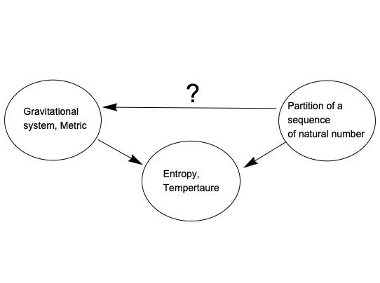
Given a configuration of black holes, there is a natural definition of entropy. On the other hand, given a sequence of natural numbers, using partition one can define entropy. Since entropy is so naturally connected with the two fields, we explore the following question in this paper. Given a sequence of natural numbers and partition, is there a direct way to get an emergent metric? Figure (2) shows the idea.

Figure 2: Since there is natural association of entropy and temperature with gravitational systems on one hand and partition of natural numbers on the other hand. Above illustration asks whether given a partition of sequence of natural numbers, is it possible to associate a metric with it?

Partition is the number of different ways of expressing a natural number as sum of smaller natural numbers. Consider following partitions

$$P\{2\} = \left\{\{2\},\{1,1\}\right\}$$

$$P\{3\} = \left\{\{3\},\{2,1\},\{1,1,1\}\right\}$$

One can think of these as degeneracy. $\{2\},\{1,1\}$ will be called parts and their set $P\{2\}=\left\{\{2\},\{1,1\}\right\}$ will be called partition. We will use the terms partition and degeneracy interchangeably. Number of parts will be denoted by $P(n)=|P\{n\}|$ . Now imagine combining $P\{2\},P\{3\}$ to form

$$P\{5\} = \left\{\{5\},\{4,1\},\{3,2\},\{3,1,1\},\{2,2,1\},\{2,1,1,1\},\{1,1,1,1,1\}\right\}$$

One part each from $P\{2\}$ and $P\{3\}$ combine (denoted by $\bullet$) to form a part of $P\{5\}$. For example, some of them are

$$\{2\}\bullet\{3\} \rightarrow \{5\}$$ (1)

$$\{2\}\bullet\{3\} \rightarrow \{3,2\}$$ (2)

$$\{2\}\bullet\{2,1\} \rightarrow \{4,1\}$$ (3)

$$\{2\}\bullet\{2,1\} \rightarrow \{3,2\}$$

$$\{2\}\bullet\{2,1\} \rightarrow \{2,2,1\}$$ (4)

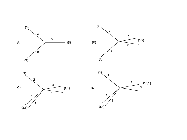
(1), (2), (3) and (4) are like three-point, four-point, five-point and six-point interaction respectively as illustrated in figure (3). This naive way of combining $P\{2\}$ and $P\{3\}$ almost produces $P\{5\}$ except some over-counting. Given $P\{n\}$ or $P(n)$, although there are formula which take close to $P\{n+1\}$ or $P(n+1)$, only way to get the exact result is to use the definition of partition.

Figure 3: (A), (B), (C) and (D) illustrate three-point, four-point, five-point and six-point interactions described in (1),(2),(3) and (4) respectively.

We will use the term interaction for combination of parts and merger for combination of partition.

When two separate systems merge into one, these interactions take place at the microscopic level. We wish to arrange the merger

$$P\{2\}\bullet P\{3\} \rightarrow....\rightarrow P\{2,3,n\}\rightarrow...\rightarrow P\{5\}$$

into a series of intermediate steps labelled by distance $n$ such that for $P\{2,3,n=\infty\}=P\{2\}\bullet P\{3\}$ (two systems are completely separate) and $P\{2,3,n=0\}=P\{5\}$ (systems have completely merged). $n$ is a measure of oneness which defines distance from complete merger. This distance emerging from interacting system defines a manifold. This is one of the main themes of the project. Interactions are fundamental from which spacetime emerges. This is opposite of treating spacetime as given and interactions happening in it. All the above discussion can be summed up as the principle of emergent causality.

Two of the sharpest predictions of the model is on information paradox(Harlow, 2016; Giddings, 1995; Mathur, 2009). While holography(Horowitz and Polchinski, 2006), soft theorems(Hawking et al., 2016; Haco et al., 2018) and other tools (Susskind, 2016; Faulkner et al., 2014; Nishioka et al., 2009; Mathur, 2008; Papadodimas and Raju, 2013) have shed light on the paradox and microstates of some black holes have also been counted (Strominger and Vafa, 1996; Sen, 2014), but puzzle is still far from being solved. When two black holes merge, gravitational radiation carry information. At least soft part of the radiation is known to carry some information (Chatterjee and Lowe, 2018). At the same time, Hawking radiation is also expected to carry information. This results in ambiguity. Does gravitational radiation and Hawking radiation, which are of classical and quantum origin respectively, both carry information, how much and what exactly is the information? This model predicts that gravitational radiation carries black-hole entropy worth of information. Secondly, we know that Hawking radiation is a result of difference in vacuum due to curved background. Energy conservation says that energy must drain out of black hole but the mechanism is still not known (Parikh, 2004; Strominger, 1994). This model suggests a clear picture of the mechanism. Another immediate question might be how does this relate to holography and stringy microstates of black hole? Please refer to the conclusion section for comments on this issue.

In an upcoming up paper we will give two experimentally verifiable predictions. Correction to Schwarzschild metric and gravitational radiation. Once measured it will let us retrieve information released during merger up-to $O(G^{3})$.

3 Outline

4 Partition

We consider the following sequence $\{m^{2}:m\in\mathbb{N}\}=\{1,4,9,16,25,...\}$. Define weighted partition $P\{m^{2},w\}$ with given weight $w\in\mathbb{{N}}$ as the following. Suppose a part is

$$m^{2} = \sum_{i}^{j}{\color[rgb]{1,0,0}\definecolor[named]{pgfstrokecolor}{rgb}{1,0,0}k_{i}}m_{i}^{2}$$

then include $W=w^{\sum_{i}^{j}{\color[rgb]{1,0,0}\definecolor[named]{pgfstrokecolor}{rgb}{1,0,0}k_{i}}}$ copies of the part in the partition. For example

$$9 = {\color[rgb]{0,1,0}\definecolor[named]{pgfstrokecolor}{rgb}{0,1,0}{\color[rgb]{1,0,0}\definecolor[named]{pgfstrokecolor}{rgb}{1,0,0}1}}\times 9={\color[rgb]{1,0,0}\definecolor[named]{pgfstrokecolor}{rgb}{1,0,0}2}\times 4+{\color[rgb]{1,0,0}\definecolor[named]{pgfstrokecolor}{rgb}{1,0,0}1}\times 1={\color[rgb]{1,0,0}\definecolor[named]{pgfstrokecolor}{rgb}{1,0,0}1}\times 4+{\color[rgb]{1,0,0}\definecolor[named]{pgfstrokecolor}{rgb}{1,0,0}5}\times 1={\color[rgb]{1,0,0}\definecolor[named]{pgfstrokecolor}{rgb}{1,0,0}9}\times 1$$

$$P\{9,w\} = \left\{\underset{w^{{\color[rgb]{1,0,0}\definecolor[named]{pgfstrokecolor}{rgb}{1,0,0}1}}}{\underbrace{\{9\},...,\{9\}}},\underset{w^{{\color[rgb]{1,0,0}\definecolor[named]{pgfstrokecolor}{rgb}{1,0,0}2+1}}}{\underbrace{\{4,4,1\},...,\{4,4,1\}}},\underset{w^{{\color[rgb]{1,0,0}\definecolor[named]{pgfstrokecolor}{rgb}{1,0,0}1+5}}}{\underbrace{\underset{5}{\left\{4,\underbrace{1,...,1}\right\}},...,\underset{5}{\left\{4,\underbrace{1,...,1}\right\}}}},\underset{w^{{\color[rgb]{1,0,0}\definecolor[named]{pgfstrokecolor}{rgb}{1,0,0}9}}}{\underbrace{\underset{9}{\left\{\underbrace{1,...,1}\right\}},...,\underset{9}{\left\{\underbrace{1,...,1}\right\}}}}\right\}$$

$$P(9,w) = w^{{\color[rgb]{1,0,0}\definecolor[named]{pgfstrokecolor}{rgb}{1,0,0}1}}+w^{{\color[rgb]{1,0,0}\definecolor[named]{pgfstrokecolor}{rgb}{1,0,0}2+1}}+w^{{\color[rgb]{1,0,0}\definecolor[named]{pgfstrokecolor}{rgb}{1,0,0}1+5}}+w^{{\color[rgb]{1,0,0}\definecolor[named]{pgfstrokecolor}{rgb}{1,0,0}9}}$$

$$P(9,w=10) = 10+10^{3}+10^{6}+10^{9}=1001001010$$

Generating function of the above partition is

$$Z = \prod_{m^{2}}\frac{1}{1-wz^{m^{2}}}$$ (6)

First thing to study about a partition is its asymptotic expansion. Asymptotic behavior is calculated as following.

$$Z(z) =\sum_{m\geq 0}P(m)z^{m} =\prod_{m\geq 1}\frac{1}{1-wz^{m^{2}}}$$ (7)

Steps of the proof follows OEIS-A006906. Product is well-defined for $|z|<1$ except for poles at $z_{k^{2}}=w^{-1/k^{2}}\alpha_{k^{2}}$ where $\alpha_{k^{2}}$ are the $\left(k^{2}\right)^{th}$ roots of unity. Coefficient $P(m^{2})$ of $z^{m^{2}}$ can be calculated by taking contour integral around $z=0$.

$$P\left(m^{2}\right) =\frac{1}{2\pi i}\oint\frac{Z(z)}{z^{m^{2}+1}} =\frac{1}{2\pi i}\oint\prod_{n\geq 1}\frac{dz}{\left(z^{m^{2}+1}\right)\left(1-wz^{n^{2}}\right)}$$

Depending on the radius of contour, integral will pick up poles. Taking circular contour, first set of poles appear at radius $|z|=w^{-1}$. This will give the leading contribution to the contour integral. Next set of poles appear at $|z|=w^{-1/4}$.

$$P\left(m^{2}\right) = \frac{1}{2\pi i}\oint_{|Z|}\frac{Z(z)dz}{\left(z^{m^{2}+1}\right)}-R\left(w^{-1}\right)$$

As we will see, residue $R(w^{-1})$ is of order $w^{m^{2}}$. Integrand inside the contour is of order $w^{m^{2}/4}$. So the contour can be anywhere between $w^{-1}<|z|<w^{-1/4}$ to get the leading contribution.

$$\lim_{m\rightarrow\infty}P\left(m^{2}\right) = -R(w^{-1})$$

$$= -\lim_{z\rightarrow w^{-1}}\frac{\left(z-w^{-1}\right)}{z^{m^{2}+1}\left(1-wz\right)}\prod_{n\geq 2}\frac{1}{1-wz^{n^{2}}}$$

$$= \lim_{z\rightarrow w^{-1}}\frac{1}{wz^{m^{2}+1}}\prod_{n\geq 2}\frac{1}{1-wz^{n^{2}}}$$

$$= w^{m^{2}}\prod_{n\geq 2}\frac{1}{1-w^{1-n^{2}}}$$

$$= r_{1}e^{G^{2}m^{2}}$$

where $r_{1}=\prod_{n\geq 2}\frac{1}{1-w^{1-n^{2}}},G^{2}=\ln w$. In this note we will assume $w=10$ whenever we want to get some estimate. For $w=10,r_{1}=1.001001011$. This is the leading behavior or the asymptotic behavior of the square partition. To calculate correction to asymptotic behavior stretch the contour to $w^{-1/4}<|z|<w^{-1/9}$. Contribution will come from next set of poles at $z_{0}=w^{-1/4}\{1,i,-1,-i\}$.

$$P\left(m^{2}\right) = -R(w^{-1})-R\left(w^{-1/4}\right)-R\left(iw^{-1/4}\right)-R\left(-w^{-1/4}\right)-R\left(-iw^{-1/4}\right)$$

$$R\left(z_{0}\right) = \lim_{z\rightarrow z_{0}}\frac{\left(z-z_{0}\right)}{z^{m^{2}+1}\left(1-wz^{4}\right)}\prod_{n\geq 1,n\neq 2}\frac{1}{1-wz^{n^{2}}}$$

$$= \lim_{z\rightarrow z_{0}}\frac{\left(z-z_{0}\right)}{wz^{m^{2}+1}\left(z-z_{0}\right)\left(z-iz_{0}\right)\left(z+z_{0}\right)\left(z+iz_{0}\right)}\prod_{n\geq 1,n\neq 2}\frac{1}{1-wz^{n^{2}}}$$

$$= -\frac{1}{wz_{0}^{m^{2}+4}\left(1-i\right)\left(1+1\right)\left(1+i\right)}\prod_{n\geq 1,n\neq 2}\frac{1}{1-wz_{0}^{n^{2}}}$$

$$= -\frac{z_{0}^{-m^{2}}}{4}\prod_{n\geq 1,n\neq 2}\frac{1}{1-wz_{0}^{n^{2}}}$$

$$R\left(w^{-1/4}\right) = -\frac{w^{m^{2}/4}}{4}\prod_{n\geq 1,n\neq 2}\frac{1}{1-w^{1-n^{2}/4}}$$

$$R\left(iw^{-1/4}\right) = -i^{m^{2}}\frac{w^{m^{2}/4}}{4}\prod_{n\geq 1,n\neq 2}\frac{1}{1-i^{n^{2}}w^{1-n^{2}/4}}$$

$$R\left(-w^{-1/4}\right) = -(-1)^{m^{2}}\frac{w^{m^{2}/4}}{4}\prod_{n\geq 1,n\neq 2}\frac{1}{1-(-1)^{n^{2}}w^{1-n^{2}/4}}$$

$$R\left(-iw^{-1/4}\right) = -(-i)^{m^{2}}\frac{w^{m^{2}/4}}{4}\prod_{n\geq 1,n\neq 2}\frac{1}{1-(-i)^{n^{2}}w^{1-n^{2}/4}}$$

If $m$ is even

$$P\left(m^{2}\right)+R(w^{-1}) = \frac{w^{m^{2}/4}}{4}$$

$$\prod_{n\geq 1,n\neq 2}\left(\frac{1}{1-w^{1-n^{2}/4}}+\frac{1}{1-i^{n^{2}}w^{1-n^{2}/4}}+\frac{1}{1-(-1)^{n^{2}}w^{1-n^{2}/4}}+\frac{1}{1-(-i)^{n^{2}}w^{1-n^{2}/4}}\right)$$

If $m$ is odd

$$P\left(m^{2}\right)+R(w^{-1}) = \frac{w^{m^{2}/4}}{4}$$

$$\prod_{n\geq 1,n\neq 2}\left(\frac{1}{1-w^{1-n^{2}/4}}+\frac{i}{1-i^{n^{2}}w^{1-n^{2}/4}}-\frac{1}{1-(-1)^{n^{2}}w^{1-n^{2}/4}}-\frac{i}{1-(-i)^{n^{2}}w^{1-n^{2}/4}}\right)$$

Thus

$$P\left(m^{2}\right) = r_{1}e^{G^{2}m^{2}}+r_{2^{2}}e^{G^{2}m^{2}/4}+O(e^{G^{2}m^{2}/9})$$

$$r_{2^{2}}=r_{4} = \begin{cases}\frac{1}{4}\prod_{n\geq 1,n\neq 2}\left(\frac{1}{1-w^{1-n^{2}/4}}+\frac{1}{1-i^{n^{2}}w^{1-n^{2}/4}}+\frac{1}{1-(-1)^{n^{2}}w^{1-n^{2}/4}}+\frac{1}{1-(-i)^{n^{2}}w^{1-n^{2}/4}}\right)&m=2k\\ \frac{1}{4}\prod_{n\geq 1,n\neq 2}\left(\frac{1}{1-w^{1-n^{2}/4}}+\frac{i}{1-i^{n^{2}}w^{1-n^{2}/4}}-\frac{1}{1-(-1)^{n^{2}}w^{1-n^{2}/4}}-\frac{i}{1-(-i)^{n^{2}}w^{1-n^{2}/4}}\right)&m=2k+1\end{cases}$$

For $w=10$

$$r_{2^{2}}=r_{4} = \begin{cases}-0.01112435883&m=2k\\ -0.00626025134&m=2k+1\end{cases}$$ (9)

Similarly one can find out higher corrections to $P\left(m^{2}\right)$. Formally it will be

$$P\left(m^{2}\right) = \sum_{n\geq 1}r_{n^{2}}e^{G^{2}m^{2}/n^{2}}$$

$$r_{w,n^{2}} = \frac{1}{n^{2}}\prod_{k\neq n}\sum_{j=1}^{n^{2}}\left(\frac{e^{2\pi j\frac{m^{2}}{n^{2}}i}}{1-e^{2\pi j\frac{k^{2}}{n^{2}}i}w^{1-\frac{k^{2}}{n^{2}}}}\right)$$

We see partition is separated into asymptotes $P_{n}(m^{2})=r_{n^{2}}e^{G^{2}m^{2}/n^{2}}$ labelled by integer $n$.

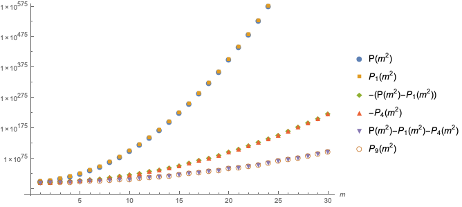
Leading asymptote $\sim e^{G^{2}m^{2}}$ is the first motivation to consider this specific form of partition. Form of $n^{th}$ subleading asymptote is $e^{G^{2}m^{2}/n^{2}}$. This is shown in figure (4). Second motivation is appearance of $n^{2}$ in the denominator in the exponent. Third motivation is weight $G$ of the partition. Their physical interpretations will become clear in the following sections.

There are two regimes. First one is the small $n$ regime where $n<Gm$. This regime is simple from partition perspective and most visible in the graph. The coefficient $r_{1}\sim P(m^{2})e^{-G^{2}m}$. On the other hand this regime is difficult because $e^{G^{2}m^{2}/n^{2}}>1$. Hence perturbative analysis is not possible. Most of the degeneracy is contained in this regime. Other is large $n$ regime $n>>Gm$. This regime represent fine deviations of partition from the leading asymptotic behavior and is difficult to see in the graph. As we will see in section (8), physical meaning of the coefficients $r_{n^{2}}$ become more and more convoluted as $n$ increases. On the other hand, since $e^{G^{2}m^{2}/n^{2}}\sim 1\implies\frac{\Delta P_{n}}{\Delta(Gm)}=r_{n^{2}}\left(\frac{2Gm}{n^{2}}\right)e^{G^{2}m^{2}/n^{2}}<<1$. So perturbative analysis is possible. Our analysis in this paper will mostly restrict to the large $n$ regime. These two regimes at the two ends of the spectrum, lies at the heart of this work as we explain in section (6). Other consequences are described in the conclusion (9).

Figure 4: Above figure has six semilog plots related to partition of squares on natural number $s(m)=\{1,4,9,...,m^{2},...:m\in\mathbb{{N}}\}$. Plot in blue dots is partition of $s(m)$. Yellow squares represent the plot of first asymptote calculated analytically. Yellow squares and blue dots can be seen to lie almost on top of each other. Green diamonds represent the difference between partition (blue dots)and the first asymptote (yellow squares). Red triangles represent second asymptote calculated analytically. Green diamonds and red triangles can be seen to lie almost on top of each other. Violet inverted triangles represent the difference between partition (blue dots)and the sum of first (yellow squares) and second (red triangles) asymptotes. Yellow circles represent third asymptote calculated analytically. Violet inverted triangles and yellow circles can be seen to lie almost on top of each other.

5 Partition Merger

We now arrange the merger of two partitions

$$P\{M^{2}\}\bullet P\{m^{2}\} \rightarrow...\rightarrow P\{M^{2},m^{2},n\}\rightarrow...\rightarrow P\{(M+m)^{2}\}$$ (10)

into a series of intermediate steps labelled by distance $n$ such that for $P\{M^{2},m^{2},n=\infty\}=P\{M^{2}\}\bullet P\{m^{2}\}$ (two systems are completely separate) and $P\{M^{2},m^{2},n=0\}=P\{(M+m)^{2}\}$ (systems have completely merged). Lets assume $M>>m$ and $P(m^{2})\sim 1$ (there is only one part), so that the process is

$$P\{M^{2}\} \rightarrow...\rightarrow P\{M^{2},m^{2},n\}\rightarrow...\rightarrow P\{(M+m)^{2}\}$$

We will call $P(m^{2})$ as test partition.

We proceed with the number of parts instead of explicit parts. In section (8) we will find out explicit parts that constitute the intermediate states and claim them to be observables. So the process we study is the following

$$P(M^{2}) \rightarrow...\rightarrow P(M^{2},m^{2},n)\rightarrow...\rightarrow P((M+m)^{2})$$ (11)

Dynamics depend on the way we define $P(M^{2},m^{2},n)$. That will also give physical meaning to $P(M^{2},m^{2},n)$ and $n$. In one step change in partition is

$$... \rightarrow P(M^{2},m^{2},n)\rightarrow P(M^{2},m^{2},n+\Delta n) \rightarrow...$$

which requires prescription for two things

1. Definition of $P(M^{2},m^{2},n)$.

2. Definition of $\Delta n\left(M^{2},m^{2},n\right)$.

Define $\Delta t\left(M^{2},m^{2},n\right)$, as change in $P_{n}$ relative to change in $P_{n}$ when $M\rightarrow M+1$.

$$\Delta t\left(M^{2},m^{2},n\right) \equiv G\left(\frac{P_{n}((M+m)^{2})-P_{n}(M^{2})}{P_{n}((M+1)^{2})-P_{n}(M^{2})}\right)$$ (12)

For $n>>m$

$$\Delta t = Gm$$

Define $P(M^{2},m^{2},n)$ and $\Delta n\left(M,m^{2},n\right)$ to be

$$P(M^{2},m^{2},n) \equiv \sum_{k\geq 1}^{n-1}P_{k}(M^{2})+\sum_{k\geq n}^{\infty}P_{k}((M+m)^{2})$$ (13)

$$\Delta v \equiv -\left(\frac{P_{n}((M+m)^{2})-P_{n}(M^{2})}{P_{n}(M^{2})}\right)$$

$$\Delta n \equiv v\Delta t$$ (14)

As an intermediate step we have defined $v$. From now on discussions will be for $n>>m$. From above prescription, when test partition is at separation $n$, degeneracy of $n^{th}$ asymptote changes

$$\Delta P_{n} = P_{n}((M+m)^{2})-P_{n}(M^{2})$$ (15)

$$= r_{n^{2}}e^{G^{2}(M+m)^{2}/n^{2}}-r_{n^{2}}e^{G^{2}M^{2}/n^{2}}$$

$$= r_{n^{2}}\left(\frac{2G^{2}Mm}{n^{2}}\right)e^{G^{2}M^{2}/n^{2}}$$

and correspondingly

$$\Delta v = -\left(\frac{\Delta P_{n}}{P_{n}}\right)$$ (16)

$$= -\frac{2G^{2}Mm}{n^{2}}$$

$$= -\frac{2GM}{n^{2}}\Delta t$$

With the condition $v(n=\infty)=0$ we get

$$v(n) = -\sqrt{\frac{2GM}{n}}$$

Let $M^{2}=\sum_{i}k_{i}m_{i}^{2}$ be a state which contributes to

$$\Delta P_{n} = \left(\frac{2G^{2}Mm}{n^{2}}\right)r_{n^{2}}e^{G^{2}M^{2}/n^{2}}$$

Before merger, states $\{m_{i}^{2}\}$ are observable and will be called space as they support the distance between the two partitions.

Upon merger, distance decreases and space is no more observable. Information $\{m_{i}^{2}\}$ is released, states $\{m_{i}^{2}\}$ become non-observable parts and degeneracy increases by $w^{\sum_{i}k_{i}}$.

$$P(M^{2},m^{2},n) \rightarrow P(M^{2},m^{2},n)+w^{\sum_{i}k_{i}}$$

In short, information associated with space is released and space is converted into parts.

Observable space $$\xrightarrow[\text{Information released}]{\text{Merger, Degeneracy increases}}$$ Non-observable parts

In other words space at radius $n$ holds

$$\Delta P_{n} = \left(\frac{2G^{2}Mm}{n^{2}}\right)r_{n^{2}}e^{G^{2}M^{2}/n^{2}}$$

amount of information. Now imagine the reverse process of sending information into $P(M^{2})$. Relative decrease of degeneracy will be

$$\left(\frac{\Delta P_{n}}{P_{n}}\right) = -\frac{2G^{2}Mm}{n^{2}}$$

As a result number of parts decrease by $\left(\frac{2G^{2}Mm}{n^{2}}\right)r_{n^{2}}e^{G^{2}M^{2}/n^{2}}$ which must be compensated by increase in space. Thus we find that sending information into the system forces partitions to de-merge. We will call this information pressure. As we discuss in conclusion, this may play an important role in Hawking radiation.

With this prescription, we can give physical meaning to the above process. If we identify $n$ with radius and $t$ with time, then equation (14) and (16) gives decrease in radius and velocity respectively. $v$ in a sense measures rate of merger With $\Delta P_{n}$ change in degeneracy, $2G^{2}Mm$ volume of space is annihilated over surface area of sphere and velocity reduces by $\frac{2G^{2}Mm}{n^{2}}$. Effectively it appears like $P\{M^{2}\}$ annihilates space of volume $2GM$ per unit time. $\frac{1}{n^{2}}$ factor in $\Delta v=\frac{2G^{2}Mm}{n^{2}}$ would give an impression that there is conservation and continuity relation and space is flowing towards the partition. As a result, space shrinks with velocity $v=\sqrt{\frac{2GM}{n}}$ and test partition drags along with the space fabric.

This would mean the system is causal as then the information released at separation $n$ and $(n+1)$ would be related. However, presence of $r_{n^{2}}$ in

$$P_{n} = r_{n^{2}}e^{G^{2}M^{2}/n^{2}}$$

invalidates this effective picture. As we show in section (8), coefficients $r_{n^{2}}$ are nothing but partitions in convoluted form. There is no exact relation between $r_{n^{2}}$ and $r_{(n+1)^{2}}$. In other words, information at separation $n$ and $(n+1)$ is not related. So there is no flow of space from radius $n+1$ to $n$. Appearance of flow is only emergent. Information released at two consecutive time slices are not related. This is how causality emerges.

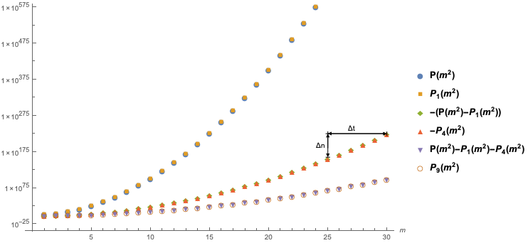
We see that time and space emerge from merger of partition. Time and space is related to the shift in the x-axis and y-axis respectively in the partition as shown in figure (5). There is no meaning of space or time without merger.

Figure 5: Above figure is same as figure 4 with additional details which shows that time emerges from difference between initial and final $m$ values and space emerges from difference in initial and final values of asymptotes.

One can ask, why to start with the sequence $\{m^{2}:m\geq 1\}=\{1,4,9,16,25,...\}$? One motivation was to get a degeneracy which grows like $\sim e^{G^{2}m^{2}}$. Now we have another completely different motivation. Suppose one had started with $\{s(m):m\geq 1\}$ where $s(m)$ is any increasing function of $m$. All the above derivation will go through with the replacements $m^{2}\rightarrow s(m),n^{2}\rightarrow s(n)$. We will end up with $\Delta n=-\frac{G^{2}s^{\prime}(M)}{s(n)}\Delta M$. However we saw that interpreting $s(n)$ as surface area of sphere gives a nice picture. This is the second motivation which connects $n^{th}$ asymptote to sphere of radius $n$.

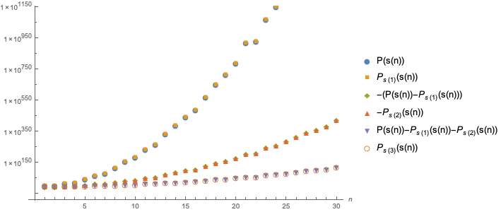
So we choose $s(n)$ to be number of integer lattice points between $n\geq r>n-1$. In other words, number of integer solutions of $n\geq\sqrt{x^{2}+y^{2}+z^{2}}>n-1$. $s=\{6,26,90,134,258,...\}$ . For $n>>1,s(n)\rightarrow 4\pi n^{2}$ which is surface area of sphere of radius $n$. This also reproduces $\Delta v=-\frac{2G^{2}Mm}{n^{2}}$ for $M,n>>1$. First few asymptotes of partition are shown in figure (6). For example, partition of $s(4)$ is

$$P{s(4),w=1}$$

$$= \Bigg{\{}\left\{134\right\},\left\{90,26,6,6,6\right\},\left\{\underset{4}{\underbrace{26,...,26}},\underset{5}{\underbrace{6,...,6}}\right\},\left\{26,\underset{18}{\underbrace{6,...,6}}\right\}\Bigg{\}}$$

$$= \Bigg{\{}\left\{s(4)\right\},\left\{s(3),s(2),s(1),s(1),s(1)\right\},\left\{\underset{4}{\underbrace{s(2),...,s(2)}},\underset{5}{\underbrace{s(1),...,s(1)}}\right\},\left\{s(2),\underset{18}{\underbrace{s(1),...,s(1)}}\right\}\Bigg{\}}$$

For all the calculation we will use $s(n)=n^{2}$. Many properties are easy to illustrate using this sequence.

Figure 6: Above figure has six semilog plots related to partition of sequence $s=\{6,26,90,134,258,...\}$ where $s(n)$ is number of integer solutions of $n\geq\sqrt{x^{2}+y^{2}+z^{2}}>n-1$. Plot in blue dots is partition of $s(n)$. Yellow squares represent the plot of first asymptote calculated analytically. They can be seen to lie almost on top of each other. Green diamonds represent the difference between partition (blue dots)and the first asymptote (yellow squares). Red triangles represent second asymptote calculated analytically. Green diamonds and red triangles can be seen to lie almost on top of each other. Violet inverted triangles represent the difference between partition (blue dots)and the sum of first (yellow squares) and second (red triangles) asymptotes. Yellow circles represent third asymptote calculated analytically. Violet inverted triangles and yellow circles can be seen to lie almost on top of each other.

Redoing the above calculation with $s(n)$ gives the following result

$$P(s(m)) = \sum_{n\geq 1}r_{s(n)}e^{G^{2}s(m)/s(n)}$$

whose generating function is

$$Z(z) =\sum_{n\geq 0}P(n)z^{n} =\prod_{n\geq 1}\frac{1}{1-wz^{s(n)}}$$

and

$$r_{w,s(n)} = \frac{1}{s(n)}\prod_{k\neq n}\sum_{j=1}^{s(n)}\left(\frac{e^{2\pi j\frac{s(m)}{s(n)}i}}{1-e^{2\pi j\frac{s(k)}{s(n)}i}w^{1-\frac{s(k)}{s(n)}}}\right)$$ (17)

Given the sequence of integer $s=\{6,26,90,134,258,...\}$, all that we have done is to study partition of these numbers. At best this contains radial evolution. How will the angular degree of freedom emerge? Given the infinite sequence $s=\{6,26,90,134,258,...\}$, $s$ is automatically mapped to solutions of $n\geq\sqrt{x^{2}+y^{2}+z^{2}}>n-1$. Thus angular information is hidden in the pattern of the infinite sequence.

6 Emergent Metric

Discussion of the previous section has set up the stage to derive the metric emerging from partition. In unit time when $P_{n}(s(M))$ changes to $P_{n}(s(M+1))$, effectively it appears like space shrinks with velocity $v=\sqrt{\frac{2GM}{n}}$ and test partition drags along with the space fabric. Goal is to show that the merger of test partition is identical to that of a fall into a black hole. There is some literature on similar issue (Czerniawski, 2006).

We start by distinguishing two frames

1. Schwarzschild frame. Coordinates are $(t_{s},n_{s},\Omega)$. $t_{s}$ is the time coordinate, $n_{s}$ is the radial coordinate which measures distance from centre of the partition and $\Omega$ is the angular coordinate. This frame coincides with the rest frame of an observer at $n_{s}=\infty$.

2. Rest frame of the test partition hovering at radial distance $n_{s}$. To stay at fixed $n_{s}$, it has to continuously boost. Coordinates are $(t_{h},n_{h},\Omega)$ which are functions of $t_{s},n_{s}$. We will call it hovering frame.

In our derivation below, we will make number of assumptions which we will prove in section 7. Metric at radial coordinate $n_{s}$ is nothing but local line element in hovering frame. Our first assumption is that boost is well defined so that hovering observer exists and line element in hovering frame is given by

$$\Delta s^{2} = -\Delta t_{h}^{2}+\Delta n_{h}^{2}$$ (18)

Non-trivial part is $-\Delta t_{h}^{2}$. $\Delta n_{h}^{2}$ follows from the choice of $s(n)$. We want to express the line element in Schwarzschild coordinates. Consider two events at $n_{s}$ ($\Delta n_{s}=0$) and separated by unit step in Schwarzschild frame. $\Delta n_{s}=0$ implies that the events are at rest in hovering frame and are boosted with respect to Schwarzschild frame. Our second assumption is that time separation in Schwarzschild frame between the events is

$$\Delta t_{s} =GE= Gm\cosh u$$ (19)

where $u=\tanh^{-1}\left(v\right),v=\sqrt{\frac{2GM}{n}}$. Information emitted in a unit step is the fundamental event and physically observable. So we assume that unit step is frame invariant. Events separated by unit step in Schwarzschild frame will also be separated by unit step in hovering frame. In hovering frame by definition $\Delta t_{h}=Gm,\Delta n_{h}=0$. So $\Delta t_{s},\Delta t_{h}$ give time interval between same two events

$$\Delta t_{h} = \frac{\Delta t_{s}}{\cosh u}=\sqrt{1-v^{2}}\Delta t_{s}$$ (20)

Consider a rod of rest length $L_{h}=L$. To stay at fixed $n_{s}$ it has to hover over $n_{s}$ and hence at rest in hovering frame. Using the above relation between time intervals and equation (18), relation between length of rod in Schwarzschild frame and hovering frame is

$$L_{h} = \frac{L_{S}}{\sqrt{1-v^{2}}}$$

$$\implies\Delta n_{h} = \frac{\Delta n_{s}}{\sqrt{1-v^{2}}}$$ (21)

Equations (20) and (21) give the relation between hovering coordinates and Schwarzschild coordinates. Substituting them in equation (18) we get

$$\Delta s^{2} = -\left(1-v^{2}\right)\Delta t_{s}^{2}+\frac{\Delta n_{s}^{2}}{1-v^{2}}+d\Omega^{2}$$ (22)

$$= -\left(1-\frac{2GM}{n}\right)\Delta t_{s}^{2}+\left(1-\frac{2GM}{n}\right)^{-1}\Delta n_{s}^{2}+d\Omega^{2}$$

Lorentz invariance of unit step is a crucial input which allows to relate events in various frames.

This is Schwarzschild metric of a black hole of mass $M$ and gravitational constant $G=\sqrt{\ln w}$. Secondly, horizon corresponds to $2GM=n$. There is no $n=0$ region as $n=1$ is the smallest natural number. Going back to partition

$$P\left(M^{2}\right) = \sum_{n\geq 1}r_{n^{2}}e^{G^{2}M^{2}/n^{2}}$$

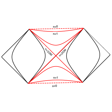
region close and far from origin is described by small $n$ regime and large $n$ regime of the partition respectively. Sharp notion of horizon enclosing all the information of black hole has disappeared. Partition is not localized within the horizon but extends all the way to the asymptotic region. There is no metric for a single partition. Metric emerges only in the context of merger of two partitions. Separate notion of matter (or black hole localized within horizon) and space-time metric (empty space far away from origin) is unified by partition. Effectively it appears as if the black hole has blurred out all over the space. We will call it blackhole-space. Notion of black hole localized in spacetime and curving it, is unified and replaced by one fundamental object blackhole-space as depicted in figure (7) and (8). This opens up the possibility of measuring the whole partition in one go as we discuss in conclusion. This establishes the following result

So far all the discussion is with natural numbers, where as in physics we deal with unitful quantities. To get unitless quantity we divide by Planck unit. For example, for $M=1kg$. Since $GM$ has units of length, it has to be divided by $l_{p}$. Leading degeneracy at $n=1$ grows like

$$P_{1}\left(M^{2}\right)=r_{1}e^{G^{2}/l_{p}^{2}}=r_{1}e^{Gc^{3}/\hbar}$$

where $l_{p}$ is Planck length. Degeneracy depends on $\hbar$ since $n$ is just a natural number independent of $\hbar$. Unitless radius of event horizon is given by $n_{h}=2GM/l_{p}=2\sqrt{\frac{Gc^{3}}{\hbar}}$. Degeneracy corresponding to $n^{th}_{h}$ asymptote is

$$P_{n_{h}}\left(M^{2}\right)=r_{n_{h}}e^{G^{2}M^{2}/n_{h}^{2}}=r_{n_{h}}e^{1/4}$$

$\hbar$ dependence in $n_{h}$ and $GM$ cancels out. So degeneracy on the surface of event horizon is independent of $\hbar$ as expected.

Now the reader may kindly read the previous boxed comments to get the physical intuition.

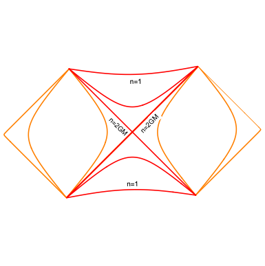
Figure 7: Penrose diagram of Schwarzschild black hole of mass $M$. $n$ is Schwarzschild radius. $n=0$ is singularity and $n=2GM$ is the horizon. Degeneracy of black hole is believed to be localized within the horizon (mostly near singularity). It is denoted by red constant $n$ slices. Information is localized within horizon. Metric sourced by the black hole extends upto asymptotic regions. This is depicted by black constant $n$ slices.

Figure 8: Penrose diagram of blackhole-space or partition $P\{M^{2}\}$. Partition ends at $n=1$ as $1$ is the smallest natural number. There is no $n=0$ region. Most of the degeneracy is localized within the small $n$ regime $n<GM$. That is depicted by red constant $n$ slices. This effectively appears like black hole with event horizon. Orange constant $n$ slices in the large $n$ regime $n>GM$ depict that degeneracy is present in this region also. Degeneracy is distributed over all $n$. There is no spacetime metric for a single partition. Metric emerges only in the context of merger of two partitions. Separate notion of black hole (degeneracy of black hole) and spacetime metric is unified and replaced by the concept of partition or blackhole-space. This whole thing is one fundamental object $P\{M^{2}\}$ that can be measured as discussed in conclusion (9).

In the above derivation we have used three assumptions: equation (18), (19) and that unit step is frame invariant. In the next section we will prove these assumptions.

7 Lorentz transformation

In the previous section we found Schwarzschild metric. One of the assumptions was energy-momentum relation. We show that as the test particle merges with black hole, the leading effect is a boost. So that by studying effect of merger on rest mass we will derive energy-momentum relation.

Leading effect of gravity is captured by equivalence principle, according to which gravity is identical to acceleration locally. Motion can be locally approximated by inertial frames and there are no local experiments which can detect gravity. In this model, angular distribution of lattice points is the local information. Taking hint from gravity, we ask the following question. What are the transformations under which this information remain invariant? In other words, what are the transformations under which angular part of line element on a sphere is invariant? We show that these transformations are isomorphic to Lorentz transformation. That will define energy-momentum relation (19) and line element (18).

Line element on a sphere is given by

$$dl^{2} = n^{2}d\theta^{2}+n^{2}\sin^{2}\theta d\phi^{2}$$

Consider the transformation

$$n = K(\theta^{\prime})n^{\prime}+O(n^{\prime-p})$$

$$\theta = g(\theta^{\prime})n^{\prime}+g^{0}(\theta^{\prime})+O(n^{\prime-p-1});p\geq 0$$

$$\phi = \phi^{\prime}$$

Throughout the discussion we will assume azimuthal symmetry. Invariance of the metric component $g_{\theta\theta}=n^{2}$ gives

$$g_{\theta^{\prime}\theta^{\prime}} = K(\theta^{\prime})^{2}n^{\prime 2}\left(\frac{dg(\theta^{\prime})}{d\theta^{\prime}}n^{\prime 2}+\frac{dg^{0}(\theta^{\prime})}{d\theta}\right)+O(n^{\prime})=n^{\prime 2}+O(n^{\prime})$$

$$\implies g(\theta^{\prime}) = c$$

$$\frac{1}{k(\theta^{\prime})} = \frac{dg^{0}(\theta^{\prime})}{d\theta}$$

Invariance of the metric component $g_{\phi\phi}=n^{2}\sin^{2}\theta$ gives

$$g_{\phi^{\prime}\phi^{\prime}} = k(\theta^{\prime})^{2}n^{\prime 2}\sin^{2}g^{0}+O(n^{\prime})=n^{\prime 2}\sin^{2}\theta^{\prime}+O(n^{\prime})$$

$$\implies\frac{dg^{0}(\theta^{\prime})}{d\theta} = \frac{\sin g^{0}}{\sin\theta^{\prime}}$$

Choosing $c=0$ we get

$$n = K(\theta^{\prime})n^{\prime}$$ (23)

$$\tan\left(\frac{g^{0}}{2}\right) = e^{-\nu}\tan\left(\frac{\theta^{\prime}}{2}\right)$$ (24)

$$K(\theta^{\prime}) = \cosh\nu+\cos\theta^{\prime}\sinh\nu$$

where $\nu$ is some constant of integration. We will call the above transformations as surface transformations.

To see the transformation of mass $m$ of test particle, the appropriate question is, how is the field of test black hole modified under above transformation? Space around test black hole of mass $m$ shrinks by $\sqrt{\frac{2Gm}{n}}$ in unit time. Hence drag velocity is

$$v^{n} = \sqrt{\frac{2Gm}{n}}$$

$$v^{\theta} = v^{\phi}=0$$

Under the above transformation

$$v^{n^{\prime}} = \frac{\partial n^{\prime}}{\partial n}v^{n}=\sqrt{\frac{2G}{n^{\prime}}\frac{m}{K^{3}}}$$ (25)

$$v^{\theta^{\prime}} = \frac{\partial\theta^{\prime}}{\partial n}v^{n}=O\left(n^{\prime-3}\right)$$

$$v^{\phi^{\prime}} = 0$$

This shows that $m$ transforms like

$$m^{\prime}(\theta^{\prime}) = \frac{m}{\left(\cosh\nu+\cos\theta^{\prime}\sinh\nu\right)^{3}}$$

Let us define

$$E\equiv m^{\prime}_{00} \equiv \int m^{\prime}Y_{00}d\Omega=m\cosh u$$

$$p_{x}\equiv m^{\prime}_{10} \equiv \int m^{\prime}Y_{10}d\Omega=m\sinh u$$

$$p_{y}\equiv m^{\prime}_{1,-1} \equiv \int m^{\prime}Y_{1,-1}d\Omega=0$$

$$p_{z}\equiv m^{\prime}_{11} \equiv \int m^{\prime}Y_{11}d\Omega=0$$

One can see that

$$E^{2}-p_{x}^{2}-p_{y}^{2}-p_{z}^{2}=m^{2}$$ (26)

is invariant under above transformation.

When a test particle of mass $m$ merges with a black hole, time elapsed in unit step is $Gm$, which is same as flux of space volume annihilated by the test particle in unit time, $\frac{1}{8\pi}\int\frac{dv^{n}}{dt}\sin\theta d\theta d\phi ndn$. This allows us to give second definition of $\Delta t$

$$\Delta t \equiv \frac{1}{8\pi}\int\frac{dv^{n}}{dt}\sin\theta d\theta d\phi ndn$$

For a Lorentz transformed test particle, flux is

$$\frac{1}{8\pi}\int\frac{dv^{n^{\prime}}}{dt}\sin\theta d\theta d\phi n^{\prime}drn^{\prime} = GE$$

Thus when boosted test particle merges with black hole, time elapsed in unit step is $GE=Gm\cosh u$. We will call $E$ as energy.

Non-vanishing higher spherical harmonics indicate that space is not annihilated isotropically.

$$m^{\prime}(\theta^{\prime}) = E+p_{x}Y_{10}+\sum_{l>1}m^{\prime}_{lm}Y_{lm}$$

For example, consider harmonics $l=0,1$. Space annihilated at $\theta=\pi$ is $E-p_{x}$ and at $\theta=0$ is $E+p_{x}$. Thus $p_{x}$ represents shift in position. We will call it momentum.

This motivates us to identify $Gm^{\prime}_{00}$ as the time element $\Delta t$ and $Gm^{\prime}_{10}$ as the length element $\Delta x$. So shift per unit time is $\frac{\Delta x}{\Delta t}=\tanh u$. For hovering frame, equating shift to drag $\sqrt{\frac{2GM}{\bar{n}}}$ gives $u=\tanh^{-1}\sqrt{\frac{2GM}{\bar{n}}}$ ($\bar{n}$ is radial coordinate of heavy black hole). This proves equation (19). Identification along with equation (26) allows us to construct invariant length

$$ds^{2} = -dt^{2}+dn^{2}+n^{2}d\theta^{2}+n^{2}\sin^{2}\theta d\phi^{2}$$ (27)

This completes the derivation of equation (18).

In addition to invariance of angular part of line element on sphere, we have to also satisfy invariance of $ds^{2}$.

$$t = a(t^{\prime},\theta^{\prime})n^{\prime}+a^{0}(t^{\prime},\theta^{\prime})+O(n^{\prime-p-1})$$

$$n = K(\theta^{\prime})n^{\prime}+\rho(t^{\prime}-n^{\prime},\theta^{\prime})+O(n^{\prime-p-1})$$

$$\theta = 2\arctan\left(e^{-\nu}\tan\frac{\theta^{\prime}}{2}\right)+O(n^{\prime-p-1});p\geq 0$$

$$\phi = \phi^{\prime}$$

Holding $t^{\prime}-n^{\prime}$ constant and for large $n^{\prime}$, above ansatz of $n$ transformation is consistent with (23) and (24).

$$g^{n^{\prime}n^{\prime}} = \left(K-\frac{d\rho}{d(t^{\prime}-n^{\prime})}\right)^{2}-a^{2}=1$$

$$g^{t^{\prime}t^{\prime}} = -\left(\frac{da}{dt^{\prime}}n^{\prime}+\frac{da^{0}}{dt^{\prime}}\right)^{2}+\left(\frac{d\rho}{d(t^{\prime}-n^{\prime})}\right)^{2}=-1$$

From second equation, comparing coefficients of $n^{\prime 2}$ gives $a=a(\theta^{\prime})$. Substituting this in first equation gives

$$\rho = (t^{\prime}-n^{\prime})\rho(\theta^{\prime})+c_{1}$$

which substituting in second equation gives

$$a^{0} = t^{\prime}a^{0}(\theta^{\prime})+c_{2}$$

So we get

$$\left(K-\rho(\theta^{\prime})\right)^{2}-a^{2} = 1$$ (28)

$$-a^{0}(\theta^{\prime})^{2}+\rho(\theta^{\prime})^{2} = -1$$ (29)

We also have third equation

$$g^{t^{\prime}n^{\prime}} = -a(\theta^{\prime})a^{0}(\theta^{\prime})+\rho(\theta^{\prime})\left(K(\theta^{\prime})-\rho(\theta^{\prime})\right)=0$$ (30)

Equations (28) and (30) give

$$a^{2}(a^{0})^{2}/\rho^{2}-a^{2} = 1$$

$$\implies-a^{0}(\theta^{\prime})^{2}+\rho(\theta^{\prime})^{2} = -\rho^{2}/a^{2}$$

$$\implies\rho^{2} = a^{2}$$

$$\implies a = \pm\rho$$

In the third step we have used equation (29). Substituting this in equation (28) gives

$$2\rho K = K^{2}-1$$

$$\implies\rho = \frac{1}{2}\left(K-\frac{1}{K}\right)$$

Substituting this in equation (30) gives

$$aa^{0} = \rho(K-\rho)$$

$$\implies a^{0} = \pm\frac{1}{2}\left(K+\frac{1}{K}\right)$$

Collecting all the results

$$t = \pm\left(Kt^{\prime}-\frac{1}{2}\left(K-\frac{1}{K}\right)(t^{\prime}-n^{\prime})\right)+c_{2}(\theta^{\prime})$$

$$n = Kn^{\prime}+\frac{1}{2}\left(K-\frac{1}{K}\right)(t^{\prime}-n^{\prime})+c_{1}(\theta^{\prime})$$

$\pm$ corresponds to just time reversal. So we choose only the $+$ solution. Undetermined functions $c_{1}(\theta^{\prime}),c_{2}(\theta^{\prime})$ are related to supertranslations. So the complete transformations are

$$t = \frac{t^{\prime}}{2}\left(K+\frac{1}{K}\right)+\frac{n^{\prime}}{2}\left(K-\frac{1}{K}\right)+c_{2}(\theta^{\prime})+O(n^{\prime-p-1})$$

$$n = \frac{n^{\prime}}{2}\left(K+\frac{1}{K}\right)+\frac{t^{\prime}}{2}\left(K-\frac{1}{K}\right)+c_{1}(\theta^{\prime})+O(n^{\prime-p-1})$$

$$\theta = 2\arctan\left(e^{-\nu}\tan\frac{\theta^{\prime}}{2}\right)+O(n^{\prime-p-1});p\geq 0$$

$$\phi = \phi^{\prime}$$

$$K(\theta^{\prime}) = \cosh\nu+\cos\theta^{\prime}\sinh\nu$$ (31)

In the direction $\theta=\theta^{\prime}=0$, above transformation is identical to Lorentz transformation with boost $-\nu$.

Some ideas in the above proof are similar to the derivation in the Bondi-Burg-Metzner-Sachs (BMS) paper (part C of (Bondi et al., 1962)). However, there are important differences in motivations, assumptions, flow of argument and result. BMS starts with Minkowski line element with $O(1/r)$ corrections and discovers that it is invariant under Lorentz transformation along with supertranslation. Motivation is to find out asymptotic symmetry group. Closely looking at the derivation one finds that there are two independent parts. First is invariance of Minkowski line element $ds^{2}=-du^{2}-2dud\tilde{r}$ under Lorentz transformation with boost $\tilde{\nu}$. Second is invariance of angular part of line element on sphere $ds^{2}=r^{2}d\theta^{2}+r^{2}\sin\theta^{2}d\phi^{2}$ under surface transformation parametrized by $\nu$. Identifying $\tilde{r}$ with $r$ implies $\tilde{\nu}=\nu$ . Gravity fixes some of the $1/r$ corrections which determines the mass transformation.

Our starting motivation is to find transformation under which local information is invariant. So we demand invariance of angular part of line element on sphere which is much weaker assumption. Then we use the velocity from partition merger and determine mass transformation. This is the keystone from which four-dimensional invariant line element follows.

8 Observables

In this section we will explore the physical meaning of the coefficients $r_{n^{2}}$ . This will help us find out partition content of the asymptote.

8.1 $r_{1}$

Let $L>>1$ denote the last element and $L_{k}$ denote the $k^{th}$ last element of the sequence $\left\{1,2,3,...,n\right\}$. Similarly, let $f(L_{k})$ denote the $k^{th}$ last element of the sequence $\left\{f(M):M\in\left\{m_{1},m_{2},...,m_{n}\right\}\right\}$. For the analytic purpose we will treat $L\rightarrow\infty$. Consider the limit $M\rightarrow L$.

$$\lim_{M\rightarrow L}P(M^{2}) = P_{1}(L^{2})$$

So define

$$r_{1} \equiv \lim_{M\rightarrow L}P(M^{2})e^{-G^{2}M^{2}}$$ (32)

which should match with the result obtained from calculating residue (4). Calculated numerically from residue, $r_{1}=1.001001011$ up to 9 decimal places. Explicit calculation of partition gives $P(n^{2}\geq 16)=1.001001011\times 10^{n^{2}}$ up to 9 decimal places. Using equation (32) we get $r_{1}=1.001001011$ for $L=16$. The two results match. Value of $L$ can be chosen based on desired accuracy. Extrapolating to finite $m$ we get

$$P_{1}(m^{2}) = \left(\lim_{M\rightarrow L}P(M^{2})e^{-G^{2}M^{2}}\right)e^{G^{2}m^{2}}$$ (33)

This gives the amount of information contained in the leading asymptote. Exact information depend on $L$. $r_{1}$ is numerically same as $P(L^{2})e^{-G^{2}L^{2}}$. Except $e^{-G^{2}L^{2}}$ which is just a multiplicative factor, information content is

$$r_{1} = P\{L^{2}\}$$

For example, if $L=16$ then information content of $r_{1}$ is partitions of $P\{16^{2}\}$.

8.2 $r_{2^{2}}$

For general $m^{2}$, equation (33) says that extrapolate $P_{1}(L^{2})$ backwards. This under-estimates $P(m^{2})$ for $m<L$. In the limit $M\rightarrow(L-1)$ we get

$$\lim_{M\rightarrow L-1}\left(P(M^{2})-P_{1}(M^{2})\right) = P_{2}((L-1)^{2})$$

Sequence $\left\{\left(P(m^{2})-P_{1}(m^{2})\right)e^{-G^{2}m^{2}/4}\right\}$ has $t_{2}=2$ subsequences $s_{2}^{t}(m)\mid\{1,4,9,...\}$, $t\in T_{2}=\{1,2,...,t_{2}\}$ with different limits.

$$\lim_{s_{2}^{t}(M)\rightarrow s_{2}^{t}(L)}\left(P(s_{2}^{t}(M))-P_{1}(s_{2}^{t}(M))\right) = P_{4}(s_{2}^{t}(L))$$

For sufficiently large $L$, $P_{4}(s_{2}^{t}(L))$ matches with $P(s_{2}^{t}(L))-P_{1}(s_{2}^{t}(L))$ up-to desired accuracy . So define

$$r_{4}^{t} \equiv \lim_{s_{2}^{t}(M)\rightarrow s_{2}^{t}(L)}\left(P(s_{2}^{t}(M))-P_{1}(s_{2}^{t}(M))\right)e^{-G^{2}s_{2}^{t}(M)/4}$$ (34)

Explicit calculation of partition for $n^{2}\geq 64$ gives

$$P(n^{2}) = \begin{cases}-0.011124359\times 10^{m^{2}/4}&m=2k\\ -0.006260251\times 10^{m^{2}/4}&m=2k+1\end{cases}$$

up to 9 decimal places. Using equation (34) we get

$$r_{2^{2}}=r_{4} = \begin{cases}-0.011124359&m=2k\\ -0.006260251&m=2k+1\end{cases}$$

This matches with the result obtained from calculating residue (9). Extrapolating to finite $m$

$$P_{2}(m^{2}) = \left(\lim_{s_{2}^{t}(M)\rightarrow s_{2}^{t}(L)}\left(P(s_{2}^{t}(M))-P_{1}(s_{2}^{t}(M))\right)e^{-Gs_{2}^{t}(M)/4}\right)e^{G^{2}m^{2}/2^{2}}$$ (35)

$$t = [m^{2}]\in T_{2}$$

where $[m^{2}]$ denote the subsequence in which $m^{2}$ appears. This gives the amount of information contained in the second asymptote.

8.3 $r_{s(1)}$

Sequence $\{P(s(m))e^{-G^{2}s(m)/s(1)}\}$ may have $t_{1}$ subsequences $s_{1}^{t}(m)\mid s(m)$, $t\in T_{1}=\{1,2,3,...,t_{1}\}$ with different limits.

$$\lim_{s(M)\rightarrow s_{1}^{t}(L)}P(s(M)) = P_{s(1)}(s_{1}^{t}(L)),t\in T_{1}$$

So define

$$r_{s(1)}^{t} \equiv \lim_{s_{1}^{t}(M)\rightarrow s_{1}^{t}(L)}P(s_{1}^{t}(M))e^{-G^{2}s_{1}^{t}(M)/s(1)},t\in T_{1}$$ (36)

which should match with the result obtained from calculating residue. One can see from the table (1) that residue matches with equation (36) for $m\geq 3$.

$m$	$r_{s(1)}\times 10^{s(m)/s(1)}$	$P(s(m))$
1	$10.00000000100010000$	$10.00000000000000000$
2	$10.00000000100010001$	$10.00000000000000000$
3	$10.00000000100010000\times 10^{15}$	$10.00000000100010000\times 10^{15}$
4	$10.00000000100010001\times 10^{19}$	$10.00000000100010001\times 10^{19}$
5	$10.00000000100010000\times 10^{43}$	$10.00000000100010000\times 10^{43}$
6	$10.00000000100010001\times 10^{65}$	$10.00000000100010001\times 10^{65}$
7	$10.00000000100010001\times 10^{79}$	$10.00000000100010001\times 10^{79}$
8	$10.00000000100010000\times 10^{115}$	$10.00000000100010000\times 10^{115}$
9	$10.00000000100010001\times 10^{157}$	$10.00000000100010001\times 10^{157}$

Table 1: Comparison of $r_{s(1)}$ and partition $P(s(1))$. Up to 17 decimal places they match for $m\geq 3$.

One can also see that up to 17 decimal places there are two limit points. Extrapolating to finite $m$

$$P_{s(1)}(s(m)) = \left(\lim_{s_{1}^{t}(M)\rightarrow s_{1}^{t}(L)}P(s_{1}^{t}(M))e^{-G^{2}s_{1}^{t}(M)/s(1)}\right)e^{G^{2}s(m)/s(1)}$$ (37)

$$t = [s(m)]\in T_{1}$$

where $[s(m)]$ denote the subsequence in which $s(m)$ appears.

8.4 $r_{s(n+1)}$

Assuming that $P_{s(n)}$ can be expressed as

$$P_{s(n)}(s(m)) = \left(\lim_{s_{n}^{u}(M)\rightarrow s_{n}^{u}(L)}\left(P(s_{n}^{u}(M))-\sum_{j=1}^{n-1}P_{s(j)}(s_{n}^{u}(M))\right)e^{-G^{2}s_{n}^{u}(M)/s(n)}\right)e^{G^{2}s(m)/s(n)},$$

$$u = [s(m)]\in T_{n}=\left\{1,2,...,t_{n}\right\}$$

where $[s(m)]$ denotes the subsequence in which $s(m)$ appear. This under-estimates $P(s_{n}^{u}(L_{k})),u\in T_{n}$ for $k>1$.

$$\lim_{{}_{s_{n}^{u}(M)\rightarrow s_{n}^{u}(L_{2})}}\left(P(s_{n}^{u}(M))-\sum_{j=1}^{n}P_{s(j)}(s_{n}^{u}(M))\right) = P_{s(n+1)}\left(s_{n}^{u}(L_{2})\right),u\in T_{n}$$

Sequence $\left\{\left(P(s_{n}^{u}(M))-\sum_{j=1}^{n}P_{s(j)}(s_{n}^{u}(M))\right)e^{-G^{2}s_{n}^{u}(M)/s(n+1)}\right\}$ has $t_{n+1}$ subsequences $s_{n+1}^{t}(m)\mid s_{n}^{u}(m)$, $t\in T_{n+1}=\{1,2,...,t_{n+1}\}$ with different limits.

$$\lim_{s_{n+1}^{t}(M)\rightarrow s_{n+1}^{t}(L)}\left(P(s_{n+1}^{t}(M))-\sum_{j=1}^{n}P_{s(j)}(s_{n+1}^{t}(m))\right) = P_{s(n+1)}(s_{n+1}^{t}(L)),t\in T_{n+1}$$

This defines $r_{s(n+1)}^{t}$

$$r_{s\left(n+1\right)}^{t} \equiv \lim_{s_{n+1}^{t}(M)\rightarrow s_{n+1}^{t}(L)}\left(P(s_{n+1}^{t}(M))-\sum_{j=1}^{n}P_{s(j)}(s_{n+1}^{t}(m))\right)e^{-G^{2}s_{n+1}^{t}(M)/s(n+1)}$$ (38)

which should match with the result obtained from calculating residue. Extrapolating to finite $m$

$$P_{s(n+1)}(s(m)) = \left(\lim_{s_{n+1}^{t}(M)\rightarrow s_{n+1}^{t}(L)}\left(P(s_{n+1}^{t}(M))-\sum_{j=1}^{n}P_{s(j)}(s_{n+1}^{t}(M))\right)e^{-G^{2}s_{n+1}^{t}(M)/s(n+1)}\right)e^{G^{2}s(m)/s(n+1)}$$

$$t = [s(m)]\in T_{n+1}=\{1,2,...,t_{n+1}\}$$ (39)

8.5 Information and Radiation

$r_{s(n)}$ was defined in section (4) as

$$P_{s(n)}(s(m)) \equiv -\sum_{i=1}^{s(n)}R(z_{i},s(m))$$ (40)

$$r_{s(n)} \equiv P_{s(n)}(s(m))e^{-G^{2}s(m)/s(n)}$$ (41)

$$R(z_{i},s(m)) = \lim_{z\rightarrow z_{0}}\frac{z-z_{i}}{z^{s(m)+1}}\prod_{l=1}^{\infty}\frac{1}{1-wz^{s(l)}}$$

$$(1-wz_{i}^{s(n)}) = 0,\forall i\in\{1,2,...,s(n)\}$$

In general, $r_{s(n)}$ takes more than one value $\{r_{s(n)}^{1},r_{s(n)}^{2},...,r_{s(n)}^{t},...,r_{s(n)}^{t_{n}}\}$ where $t$ depends on $s(m)$.
Another way to define $r_{s(n)}^{t}$ is using equation (38). We motivated and also checked numerically the definition (39) matches with (40) for finite $m$. While (40) and (41) are calculated using finite number of initial terms of partition $\{P(s(1)),P(s(2)),....,P(s(m))\}$. (38) and (39) are calculated using finite number of end terms of partition $\{P(s(L)),P(s(L_{2})),....,P(s(L_{m}))\}$. These definitions extrapolated to finite $m$ match with each other.

The second definition has the advantage of being physically meaningful. It tells us that $r_{n^{2}}$ is nothing but partition. Along with this knowledge, $\Delta P_{n}$ in equation (15) gives observable information. Since this observable information is a result of change in background metric, it is nothing but bremsstrahlung radiation. Still some work is necessary to find out the exact form of the gravitational radiation. That will be done in a follow up paper.

9 Conclusion

We have considered a model based on partition of squares $\{1,4,9,...,m^{2},...:m\in\mathbb{{N}}\}$ with weight $w=e^{G^{2}}$ as defined in section (4). It can be expressed as sum of asymptotes

$$P\left(m^{2}\right) = \sum_{n\geq 1}P_{n}(m^{2})$$

$$P_{n}(m^{2}) = r_{n^{2}}e^{G^{2}m^{2}/n^{2}}$$

$$r_{w,n^{2}} = \frac{1}{n^{2}}\prod_{k\neq n}\sum_{j=1}^{n^{2}}\left(\frac{e^{2\pi j\frac{m^{2}}{n^{2}}i}}{1-e^{2\pi j\frac{k^{2}}{n^{2}}i}w^{1-\frac{k^{2}}{n^{2}}}}\right)$$

Leading asymptote grows like $e^{G^{2}m^{2}}$ and $n^{th}$ subleading asymptote grows like $e^{G^{2}m^{2}/n^{2}}$ . There are two different regimes. First is small $n$ regime $n<Gm$. This regime is closer to partition perspective and most visible in the graph (4). The coefficient $r_{1}$ has simple physical interpretation in terms of partition as described in section (8). On the other hand since $e^{G^{2}m^{2}/n^{2}}>1$, perturbative analysis is not possible. Second is large $n$ regime $n>>Gm$. This regime represent fine deviations of partition from the leading asymptotic behavior and is difficult to see in the graph. Coefficients $r_{n^{2}}$ become more and more complicated for $n>>Gm$. On the other hand, $e^{G^{2}m^{2}/n^{2}}\sim 1\implies\frac{\Delta P_{n}}{\Delta(Gm)}=r_{n^{2}}\left(\frac{2G^{2}m}{n^{2}}\right)e^{G^{2}m^{2}/n^{2}}<<1$. So perturbative analysis is possible.

We have studied merger of two partitions and realized that the amount of merger can be used as a measure to define distance $n$.

$$P\{m^{2}\}\bullet P\{M^{2}\} \rightarrow P\{m^{2},M^{2},n\}\rightarrow P\{(M+m)^{2}\}$$

such that $P\{m^{2},M^{2},n=\infty\}=P\{m^{2}\}\bullet P\{M^{2}\}$ (two systems are completely separate) and $P\{m^{2},M^{2},n=0\}=P\{(M+m)^{2}\}$ (systems have completely merged). When intermediate state $P\{m^{2},M^{2},n\}$ is identified with the $n^{th}$ subleading asymptote then merger matches with particle falling in black hole. Space and time acquires meaning only in the context of merger. Prior to merger parts are observable which are called space. Upon merger, space is converted to non-observable parts and information is released. As a result, space shrinks with velocity $v=\sqrt{\frac{2GM}{n}}$ at radius $n$ from the black hole and test particle drags along with the space fabric.

Effective physical picture emerges where a black hole of mass $M$ acts as space sink and annihilates space of volume $2GM$ per unit time. Specially $\frac{1}{n^{2}}$ factor in $\Delta v=\frac{2GM}{n^{2}}\Delta t$ would give an impression that there is conservation and continuity relation. Space is flowing towards black hole and finally draining into it. However information emitted during merger from surface of radius $n$

$$\Delta P_{n} = r_{n^{2}}\left(\frac{2G^{2}Mm}{n^{2}}\right)e^{G^{2}M^{2}/n^{2}}$$

reveals that the effective picture is misleading. Discussion in section (8) shows that coefficients $r_{n^{2}}$ are nothing but partitions in convoluted form. Thus there is no analytic relation between $r_{n^{2}}$ and $r_{(n+1)^{2}}$. To get $\Delta P_{n}$ one has to fall back to the definition of partition. In other words, information on surface of radius $n$ and $(n+1)$ is not related. So there is no flow of space from one surface to the next. Appearance of flow is only emergent. Information released at two consecutive time slices are unrelated. This is how causality emerges. Emergent causality is the guiding principle throughout the work. Place where emergent patterns are found is Natural numbers or some derivative of it. So we call this framework Sankhyaa (pronounced Sunkh-ya).

Majority of the information is contained in small $n$ asymptotes. Information appears to be localized in a bounded region which effectively looks like an event horizon. Region inside and far outside the horizon is described by small $n$ and large $n$ asymptotes respectively. The sharp notion of event horizon disappears and information is spread all over the space. This unifies black hole and background spacetime and replaces them with one fundamental object described by partition. We call it blackhole-space. Small $n$ regime is closer to black-hole entropy and large $n$ regime is closer to spacetime perspective. Important take away is that one mechanism explains black-hole entropy and metric. This shows that gravitational radiation carries black-hole entropy worth of information. By analyzing the radiation we can retrieve the information emitted during merger. In a follow up paper we will give corrections to Schwarzschild metric and gravitational radiation from which information can be retrieved upto $O(G^{3})$. Second prediction is that if radiation with right information is sent in, instead of increasing mass of black hole it will de-merge the black hole. This is reverse process of black-hole formation. That is how, a free particle is able to resist fall by boosting in opposite direction. We call this phenomenon as information pressure. This will be shown in future work.

From the above model it is clear that classical gravity cannot be separated from quantum gravity. Gravity is quantized from the get-go. The root lies in common origin of metric (large $n$ regime) and black-hole entropy (small $n$ regime). Metric is usually assumed to have classical meaning as in classical general relativity, while entropy is purely quantum object without any classical description. This work shows that metric and entropy are on equal footing. There is no meaning of metric without entropy. This was expected a-priori for at least couple of reasons. First reason comes from information puzzle. Black-hole entropy is of quantum origin. On the other hand soft radiation is known to carry to some information (Chatterjee and Lowe, 2018; Hawking et al., 2016). This is classical in nature. Hence there is some ambiguity between classical and quantum origin of information. Secondly, in emergent causality, boundary condition is built into the system. This can also be seen as unification of boundary condition with the differential equation. Any attempt to unify differential equation with boundary conditions will quantize the theory. Hence the system is quantized by construction. This is one of the hallmarks of quantum gravity.

A comprehensive discussion of information paradox and associated confusions and subtleties can be found in (Harlow, 2016; Mathur, 2009). While the spectrum of approaches is very broad, all of them have one feature in common. They all interpret information as quantum information. That is, all the approaches are based on qubits / quantum fields / wavefunction which we will collectively refer to as field. Original Hawking’s argument of mixed nature of radiation is also formulated in terms of quantum field. Field by definition requires a pre-notion of spacetime. In some sense, the knot of information paradox lies at lack of correct understanding of what do we mean by information?

Information content and interpretation is very different for a bit (classical information) and a qubit. While separate classical bits describe position and momentum, quantum field contains information about both position and momentum. Bit cannot be used to describe qubit. Just like qubit and bit are two completely different ways of describing nature. In the same way, partition of natural numbers is a completely new way of describing nature. Separate quantum fields are necessary to describe matter and metric. Partition integrates information about the particle and the spacetime by unifying them. Bits or qubits cannot be used to describe partition. Instead of wavefunction of black hole, partition of blackhole-space is more apt description of nature. This work can also be seen as an interpretation of partition. We found the prescription through which classical information emerges from partition. More detailed study is necessary to see how field emerges from partition.

Seen as scattering process, Hawking radiation is a spontaneous decay process of black hole. Above model allows de-merger of black hole if right information is sent into the black hole. This suggests a mechanism by which energy can flow out of black hole. In future work we would like to explore these issues.

There is also a volume of work on stringy microstates of black hole summed up in (Sen, 2014). These microstates count the number of excitations of string in weak coupling limit. In perturbative string theory, strings or branes are D-dimensional fundamental objects leaving in spacetime. Partition or blackhole-space is also an extended fundamental object by itself. But it does not exist inside spacetime. It is unified description of spacetime and matter together. It is different from counting string states. Partition is like degrees of freedom in natural numbers. At best one can think of the parts as excitation of gravitons or degrees of freedom of spacetime. Probably this work will have natural connection with non-perturbative description of string theory.

Experiments in physics are about observing field and radiation far from the particle. This is same as measuring large $n$ asymptotes of the partition. From that we reconstruct properties of the particle. This is the only known way of observing nature till now. We do not see the particle as whole. This work suggests that there could be experiments for small $n$ regime as well, which would be new class of experiments closer to partition perspective and far from spacetime perspective. A stronger claim is that it could be possible to see the whole particle if one can capture the full partition $P\{n^{2}\}$ (this is exact partition and not just the leading asymptotes) in one go. This would be completely new way of observing nature devoid of space and time. Experimental aspects of partition will be demonstrated in future project.