Abstract

Recently the RBC-UKQCD lattice QCD collaboration presented new results for the hadronic matrix elements relevant for the ratio $\varepsilon^{\prime}/\varepsilon$ in the Standard Model (SM) albeit with significant uncertainties. With the present knowledge of the Wilson coefficients and isospin breaking effects there is still a sizable room left for new physics (NP) contributions to $\varepsilon^{\prime}/\varepsilon$ which could both enhance or suppress this ratio to agree with the data. The new SM value for the $K^{0}-\bar{K}^{0}$ mass difference $\Delta M_{K}$ from RBC-UKQCD is on the other hand by $2\sigma$ above the data hinting for NP required to suppress $\Delta M_{K}$. Simultaneously the most recent results for $K^{+}\rightarrow\pi^{+}\nu\bar{\nu}$ from NA62 and for $K_{L}\rightarrow\pi^{0}\nu\bar{\nu}$ from KOTO still allow for significant NP contributions. We point out that the suppression of $\Delta M_{K}$ by NP requires the presence of new CP-violating phases with interesting implications for $K\to\pi\nu\bar{\nu}$, $K_{S}\to\mu^{+}\mu^{-}$ and $K_{L}\to\pi^{0}\ell^{+}\ell^{-}$ decays. Considering a $Z^{\prime}$-scenario within the SMEFT we analyze the dependence of all these observables on the size of NP still allowed by the data on $\varepsilon^{\prime}/\varepsilon$. The hinted $\Delta M_{K}$ anomaly together with the $\varepsilon_{K}$ constraint implies in the presence of only left-handed (LH) or right-handed (RH) flavour-violating $Z^{\prime}$ couplings strict correlation between $K^{+}\rightarrow\pi^{+}\nu\bar{\nu}$ and $K_{L}\rightarrow\pi^{0}\nu\bar{\nu}$ branching ratios so that they are either simultaneously enhanced or suppressed relative to SM predictions. An anticorrelation can only be obtained in the presence of both LH and RH couplings. Interestingly, the NP QCD penguin scenario for $\varepsilon^{\prime}/\varepsilon$ is excluded by SMEFT renormalization group effects in $\varepsilon_{K}$ so that NP effects in $\varepsilon^{\prime}/\varepsilon$ are governed by electroweak penguins. We also investigate for the first time whether the presence of a heavy $Z^{\prime}$ with flavour violating couplings could generate through top Yukawa renormalization group effects FCNCs mediated by the SM $Z$-boson. The outcome turns out to be very interesting.

1 Introduction

The ratio $\varepsilon^{\prime}/\varepsilon$ that measures the size of direct CP violation in $K_{L}\to\pi\pi$ decays relative to the indirect CP violation described by $\varepsilon_{K}$ and the rare decays $K^{+}\rightarrow\pi^{+}\nu\bar{\nu}$ and $K_{L}\rightarrow\pi^{0}\nu\bar{\nu}$ have been already for many years together with the $\Delta I=1/2$ rule, $K_{L,S}\to\mu^{+}\mu^{-}$ and $K_{L}\to\pi^{0}\ell^{+}\ell^{-}$ decays the stars of Kaon flavour physics [1]. The $K_{L}$–$K_{S}$ mass difference $\Delta M_{K}$ remained due to large theoretical uncertainties until recently under the shadow of these decays although it played a very important role in the past in estimating successfully the charm quark mass prior to its discovery [2]. However, recently progress in evaluating $\Delta M_{K}$ within the SM has been made by the RBC-UKQCD collaboration [3, 4, 5] so that $\Delta M_{K}$ begins to play again an important role in phenomenology, not only to bound effects of NP contributions [6, 7, 8, 9, 10, 11], but also to help identify what this NP could be. But as stressed in [1] and in particular in [12] such an identification is only possible by considering all the stars of Kaon physics simultaneously and also invoking observables from other meson systems.

The RBC-UKQCD lattice QCD collaboration presented very recently new results for the hadronic matrix elements relevant for the ratio $\varepsilon^{\prime}/\varepsilon$. Using the Wilson coefficients at the NLO level and not including isospin breaking and NNLO QCD effects they find [13]

$$(\varepsilon^{\prime}/\varepsilon)_{\rm SM} =(21.7\pm 8.4)\times 10^{-4}\,,$$ (1)

where statistical, parametric and systematic uncertainties have been added in quadrature.

However, as already demonstrated in [14], the inclusion of the effects in question, that are absent in (1) is important. Including the isospin breaking contributions, recently calculated in [15] and the NNLO QCD corrections to electroweak penguin contributions [16], the result in (1) is changed to [15, 17]

$$(\varepsilon^{\prime}/\varepsilon)_{\rm SM} =(13.9\pm 5.2)\times 10^{-4}\,,$$ (2)

which compared with the experimental world average from NA48 [19] and KTeV [20, 21] collaborations,

$$(\varepsilon^{\prime}/\varepsilon)_{\text{exp}} =(16.6\pm 2.3)\times 10^{-4}\,,$$ (3)

shows a very good agreement of the SM with the data, albeit leaving still much room for NP contributions. Presently values as low as 5 or as high as 25 in these units cannot be excluded.

While this result allows for both positive and negative NP contributions to $\varepsilon^{\prime}/\varepsilon$ to agree with the data, the new SM value for the $K^{0}-\bar{K}^{0}$ mass difference $\Delta M_{K}$ from RBC-UKQCD [5]

$$(\Delta M_{K})_{\text{SM}}=7.7(2.1)\times 10^{-15}\,{\rm GeV},\qquad(\Delta M_{K})_{\text{exp}}=3.484(6)\times 10^{-15}\,{\rm GeV}\,,$$ (4)

hints at the $2\sigma$ level at the presence of NP required to suppress $\Delta M_{K}$ relative to its SM value.

As noted already in [12] the suppression of $\Delta M_{K}$ is only possible in the presence of new CP-violating couplings. This could appear surprising at first sight, since $\Delta M_{K}$ is a CP-conserving quantity but simply follows from the fact that the BSM shift $(\Delta M_{K})_{\text{BSM}}$ is proportional to the square of a complex $g_{sd}$ coupling so that

$$(\Delta M_{K})_{\text{BSM}}=c~{}\rm{Re}[g_{sd}^{2}]=c\left[(\rm{Re}[g_{sd}])^{2}-(\rm{Im}[g_{sd}])^{2}\right],\qquad c>0.$$ (5)

The required negative contribution implies automatically NP contributions to $\varepsilon^{\prime}/\varepsilon$ and also to rare decays $K\to\pi\nu\bar{\nu}$, $K_{S}\to\mu^{+}\mu^{-}$ and $K_{L}\to\pi^{0}\ell^{+}\ell^{-}$, provided this NP involves non-vanishing flavour conserving $q\bar{q}$ couplings in the case of $\varepsilon^{\prime}/\varepsilon$ and non-vanishing $\nu\bar{\nu}$ and $\mu^{+}\mu^{-}$ couplings in the case of the rare $K$ decays in question.

Now, as pointed out in an important paper by Monika Blanke eleven years ago [22], in the presence of a strict correlation between NP contributions to $\Delta S=1$ and $\Delta S=2$ processes and assuming no significant NP contributions to $\varepsilon_{K}$ implies two narrow branches in the $(K^{+}\rightarrow\pi^{+}\nu\bar{\nu},K_{L}\rightarrow\pi^{0}\nu\bar{\nu})$ plane , namely

• a branch parallel to the Grossman-Nir (GN) bound [23] on which both branching ratios can either simultaneously increase or decrease relative to SM values,

• a horizontal narrow branch on which there is no NP contribution to $K_{L}\rightarrow\pi^{0}\nu\bar{\nu}$ because of the absence of flavour-violating complex couplings.

This is in particular the case of NP entering already at tree-level with only left-handed or right-handed flavour-violating NP couplings with the prominent example of $Z^{\prime}$ models in which the $Z^{\prime}\bar{s}d$ coupling enters both $K^{+}\rightarrow\pi^{+}\nu\bar{\nu}$ and $K_{L}\rightarrow\pi^{0}\nu\bar{\nu}$ as well as $\varepsilon_{K}$.

The hinted anomaly in $\Delta M_{K}$, requiring the imaginary couplings to be present, excludes the horizontal branch so that the full action of NP in this case happens only on the second branch to be called MB-branch in what follows.

But in [22] a possible impact of $\Delta M_{K}$ has not been discussed. Therefore, under the assumption of significant NP contributions to $\varepsilon_{K}$ but still considering only scenarios with left-handed or right-handed flavour-violating $Z^{\prime}$ couplings leads to significantly broader branches than when $\varepsilon_{K}$ from the SM agreed with the data. However, as we will demonstrate in the present paper, the removal of the $\Delta M_{K}$ anomaly combined with renormalization group Yukawa top effects implies still a rather narrow MB-branch.

In this context it is interesting to observe that the most recent result for $K^{+}\rightarrow\pi^{+}\nu\bar{\nu}$ from NA62 [24] and the $90\%$ confidence level (CL) upper bound on $K_{L}\rightarrow\pi^{0}\nu\bar{\nu}$ from KOTO [25] read respectively

$$\mathcal{B}(K^{+}\rightarrow\pi^{+}\nu\bar{\nu})_{\text{exp}}=(4.7^{+7.2}_{-4.7})\times 10^{-11}\,,\qquad\mathcal{B}(K_{L}\rightarrow\pi^{0}\nu\bar{\nu})_{\text{exp}}\leq 3.0\times 10^{-9}\,,$$ (6)

to be compared with the SM predictions [26, 27]

$$\mathcal{B}(K^{+}\rightarrow\pi^{+}\nu\bar{\nu})_{\text{SM}}=(8.5^{+1.0}_{-1.2})\times 10^{-11}\,,\qquad\mathcal{B}(K_{L}\rightarrow\pi^{0}\nu\bar{\nu})_{\text{SM}}=(3.2^{+1.1}_{-0.7})\times 10^{-11}\,.$$ (7)

In their most recent status report [28] on $K_{L}\rightarrow\pi^{0}\nu\bar{\nu}$ the KOTO collaboration presented data on four candidate events in the signal region, finding

$$\mathcal{B}(K_{L}\rightarrow\pi^{0}\nu\bar{\nu})_{\text{KOTO}}=2.1^{+2.0(+4.1)}_{-1.1(-1.7)}\times 10^{-9}\,,$$ (8)

at the 68 (95) % CL. The central value is by a factor of 65 above the central SM prediction and in fact violates the GN bound which at the $90\%$ CL together with the present NA62 result for $K^{+}\rightarrow\pi^{+}\nu\bar{\nu}$ amounts to $0.8\times 10^{-9}$. Theoretical analyses of this interesting data can be found in [29, 30, 31, 32].

Evidently there is still much room for NP left in these decays. In particular, a pattern in which $K^{+}\rightarrow\pi^{+}\nu\bar{\nu}$ is suppressed and $K_{L}\rightarrow\pi^{0}\nu\bar{\nu}$ is enhanced by NP is hinted by the new data. As pointed out already in [22] and seen in the plots in [22, 33] this pattern is only possible in the presence of both left-handed and right-handed flavour-violating $Z^{\prime}$ couplings to quarks which with moderate fine-tuning allows to avoid the constraint from $\varepsilon_{K}$, so that regions in the $(K^{+}\rightarrow\pi^{+}\nu\bar{\nu},K_{L}\rightarrow\pi^{0}\nu\bar{\nu})$ plane outside the MB-Branch are possible. We will return to this issue in Section 4.3, but we stress already here, following [22], that generally in NP scenarios in which NP contributions to $\Delta S=1$ and $\Delta S=2$ are not related to each other, different oases in the $(K^{+}\rightarrow\pi^{+}\nu\bar{\nu},K_{L}\rightarrow\pi^{0}\nu\bar{\nu})$ plane outside the MB-Branch could be occupied. As evident from the plots in [34, 33] the simplest example are models with minimal flavour violation (MFV). There the correlation between $K^{+}\rightarrow\pi^{+}\nu\bar{\nu}$ and $K_{L}\rightarrow\pi^{0}\nu\bar{\nu}$ results from the same real valued loop function $X$ entering these two processes. This function is a priori unrelated to NP contributions in $\Delta S=2$ processes and therefore $\Delta S=2$ constraints are avoided. On the other hand in the absence of new complex flavour-violating phases in MFV models the suppression of $\Delta M_{K}$ is not possible. This is reminiscent of lower bounds on $\Delta M_{s,d}$ present in these models [35, 36].

It has been pointed out already in [12] that various patterns of NP in rare $K$ decays in correlation with NP in $\varepsilon^{\prime}/\varepsilon$ can naturally be realized in models with tree-level FCNCs mediated by a heavy $Z^{\prime}$ with masses still in the reach of ATLAS and CMS but also for higher masses. But whereas in [12] the scenarios with enhanced $K^{+}\rightarrow\pi^{+}\nu\bar{\nu}$ and $K_{L}\rightarrow\pi^{0}\nu\bar{\nu}$ have been primarily considered, a novel pattern in which $K^{+}\rightarrow\pi^{+}\nu\bar{\nu}$ is suppressed and $K_{L}\rightarrow\pi^{0}\nu\bar{\nu}$ is enhanced by NP possibly hinted by the new data has not been considered there.

With the new information from RBC-UKQCD on $\varepsilon^{\prime}/\varepsilon$ and $\Delta M_{K}$, the new analyses of $\varepsilon^{\prime}/\varepsilon$ in [15, 17] and the new data from NA62 and KOTO, it is of interest to ask how the $Z^{\prime}$ scenarios considered in [12] and the new ones face the new developments listed above.

The goal of the present paper is to answer this question, but our paper should not be considered as the numerical update of the analysis in [12] motivated by the new input from RBC-UKQCD, NA62 and KOTO collaborations. The reason is that in contrast to [12], that included only QCD renormalization group effects, we will perform a complete SMEFT analysis, that takes in particular into account important top Yukawa effects, which modify significantly the properties of a $Z^{\prime}$ responsible for the pattern of NP effects in question. In particular we point out that the so-called QCD penguin scenario for $\varepsilon^{\prime}/\varepsilon$, considered in [12], in which at the NP scale only QCD penguin operators have non-vanishing Wilson coefficients, is excluded due to Yukawa renormalization group effects on $\varepsilon_{K}$ when NP contributions to $\varepsilon^{\prime}/\varepsilon$ and $\Delta M_{K}$ are considered simultaneously. We demonstrate this effect both analytically and numerically.

In models with vector-like quarks the operators $\psi^{2}H^{2}D$, listed in Table 5, are generated at the matching scale, implying FCNCs mediated by the SM $Z$-boson. They can be enhanced through RG Yukawa top quark effects with an important impact on the phenomenology [27, 37, 38]. Such operators have vanishing Wilson coefficients in $Z^{\prime}$ models at tree-level if the $(H^{\dagger}iD_{\mu}H)Z_{\mu}^{\prime}$ coupling is set to zero. However, they are generated again through RG Yukawa top quark effects. To our knowledge this mechanism of generating FCNCs mediated by the $Z$ in $Z^{\prime}$ models has not been considered in the literature. Usually the FCNCs in $Z^{\prime}$ models are generated through $Z-Z^{\prime}$ mixing in the process of the spontaneous breakdown of the electroweak symmetry [39]. It is then of interest to investigate whether this pure RG effect is important.

Our paper is organized as follows. In Section 2 we recall the strategy of [12] where the correlations between $\varepsilon^{\prime}/\varepsilon$, $\Delta M_{K}$, $K^{+}\rightarrow\pi^{+}\nu\bar{\nu}$ and $K_{L}\rightarrow\pi^{0}\nu\bar{\nu}$ have been analyzed in the framework of $Z^{\prime}$ models taking into account the constraints from $K_{L}\to\mu^{+}\mu^{-}$ and $\varepsilon_{K}$. We refrain, with the exception of $\varepsilon^{\prime}/\varepsilon$, from listing the formulae for observables entering our analysis as they can be found in [12] and in more general papers on $Z^{\prime}$ models in [40] and in [41] that deals with 331 models. On the other hand we discuss in some detail the aspects of new dynamics that enrich the analysis of [12] through the inclusion of the full machinery of the SMEFT, in particular of the renormalization group effects from top Yukawa coupling.

In Section 3 as a preparation for the numerical analysis we discuss various $Z^{\prime}$ scenarios and the related RG evolution patterns in the SMEFT.

In Section 4 we present a detailed numerical analysis of all observables listed above, including also $K_{S}\to\mu^{+}\mu^{-}$ and $K_{L}\to\pi^{0}\ell^{+}\ell^{-}$, in various $Z^{\prime}$ scenarios.

In Section 5 we analyze the generation of FCNCs mediated by the SM $Z$-boson. In Section 6 we list the main results of our paper and present a brief outlook for the coming years. Some additional information is contained in an appendix.

2 Basic Formalism

2.1 Strategy

In our paper, as in [12], an important role will be played by $\varepsilon^{\prime}/\varepsilon$ and $\varepsilon_{K}$ for which in the presence of NP contributions, to be called BSM in what follows, we have

$$\frac{\varepsilon^{\prime}}{\varepsilon}=\left(\frac{\varepsilon^{\prime}}{\varepsilon}\right)^{\rm SM}+\left(\frac{\varepsilon^{\prime}}{\varepsilon}\right)^{\rm BSM}\,,\qquad\varepsilon\equiv\varepsilon_{K}=e^{i\phi_{\epsilon}}\,\left[\varepsilon_{K}^{\rm SM}+\varepsilon^{\rm BSM}_{K}\right]\,.$$ (9)

In view of uncertainties present still in the SM estimates of $\varepsilon^{\prime}/\varepsilon$, and to a lesser extent in $\varepsilon_{K}$, we will fully concentrate on BSM contributions. Therefore in order to identify the pattern of BSM contributions to flavour observables implied by allowed BSM contributions to $\varepsilon^{\prime}/\varepsilon$ in a transparent manner, we will proceed in a given $Z^{\prime}$ scenario as follows [12]:

Step 1: We assume that BSM provides a shift in $\varepsilon^{\prime}/\varepsilon$:

$$\left(\frac{\varepsilon^{\prime}}{\varepsilon}\right)^{\rm BSM}=\kappa_{\varepsilon^{\prime}}\cdot 10^{-3},\qquad-1.0\leq\kappa_{\varepsilon^{\prime}}\leq 1.0,$$ (10)

with the range for $\kappa_{\varepsilon^{\prime}}$ indicating conservatively the room left for BSM contributions. This range is dictated by the recent analyses in [15, 17] which implies the result quoted in (2). Specifically, we will consider three ranges for $\kappa_{\varepsilon^{\prime}}$

$$(\text{A})\quad 0.5\leq\kappa_{\varepsilon^{\prime}}\leq 1.0,\qquad(\text{B})\quad-0.5\leq\kappa_{\varepsilon^{\prime}}\leq 0.5,\qquad(\text{C})\quad-1.0\leq\kappa_{\varepsilon^{\prime}}\leq-0.5.$$ (11)

Only range A has been considered in [12] so that the study of ranges B and C is new with interesting consequences.

This step will determine for given flavour conserving $Z^{\prime}\bar{q}q$ couplings the imaginary parts of flavour-violating $Z^{\prime}$ couplings to quarks as functions of $\kappa_{\varepsilon^{\prime}}$. But as we will see below in order to explain the $\Delta M_{K}$ anomaly, which requires significant imaginary couplings, and simultaneously obtain $\varepsilon^{\prime}/\varepsilon$ consistent with the ranges above the flavour conserving $Z^{\prime}\bar{q}q$ couplings must be $\mathcal{O}(10^{-2})$.

We stress even stronger the usefulness of $\kappa_{\varepsilon^{\prime}}$ in the 2020s than it could be anticipated in [12]. The result in (2) governed by the hadronic matrix elements from the RBC-UKQCD collaboration has a very large error and we expect that it will still take some time before this error will be decreased down to $10-15\%$. In addition we need a second lattice group to confirm the 2020 RBC-UKQCD value and it is not evident that this will happen in this decade.

Step 2: In order to determine the relevant real parts of the couplings involved, in the presence of the imaginary part determined from $\varepsilon^{\prime}/\varepsilon$, we will assume that BSM can also affect the parameter $\varepsilon_{K}$. We will describe this effect by the parameter $\kappa_{\varepsilon}$ so that now in addition to (10) we will allow for a BSM shift in $\varepsilon_{K}$ in the range

$$(\varepsilon_{K})^{\rm BSM}=\kappa_{\varepsilon}\cdot 10^{-3},\qquad-0.2\leq\kappa_{\varepsilon}\leq 0.2\,.$$ (12)

This is consistent with present analyses in [42, 43, 44]. But it should be stressed that this depends on whether inclusive or exclusive determinations of $|V_{ub}|$ and $|V_{cb}|$ are used and with the inclusive ones the SM value of $\varepsilon_{K}$ agrees well with the data. We will also investigate how our results change when a larger NP contribution to $\varepsilon_{K}$ corresponding to $-0.5\leq\kappa_{\varepsilon}\leq 0.5$ is admitted.

Step 3: As far as $\Delta M_{K}$ is concerned, we will consider dominantly NP parameters which provide the suppression of the SM value in accordance with the LQCD result in (4). In particular this will require the imaginary $Z^{\prime}$ couplings to be significantly larger than the real ones.

Step 4: In view of the uncertainty in $\kappa_{\varepsilon^{\prime}}$ we set several parameters to their central values. In particular for the SM contributions to rare decays we set the CKM factors and the CKM phase $\delta$ to

$${\rm Re}\lambda_{t}=-3.4\cdot 10^{-4},\qquad{\rm Im}\lambda_{t}=1.48\cdot 10^{-4}\,,\qquad\delta=1.27\,,$$ (13)

which are close to the central values of present estimates obtained by the UTfit [42] and CKMfitter [43] collaborations. For this choice of CKM parameters the central value of the resulting $|\varepsilon_{K}^{\rm SM}|$ is $2.32\cdot 10^{-3}$. With the experimental value of $\varepsilon_{K}$ in Table 3 this implies $\kappa_{\varepsilon}=-0.09$ . But we will still vary $\kappa_{\varepsilon}$ while keeping the values in (13), as BSM contributions in our scenarios do not depend on them but are sensitive functions of $\kappa_{\varepsilon}$.

Step 5: Having fixed the flavour violating couplings of the $Z^{\prime}$ in this manner, we will be able to calculate BSM contributions to the branching ratios for $K^{+}\rightarrow\pi^{+}\nu\bar{\nu}$, $K_{L}\rightarrow\pi^{0}\nu\bar{\nu}$, $K_{L,S}\to\mu^{+}\mu^{-}$ and $K_{L}\to\pi^{0}\ell^{+}\ell^{-}$ and to $\Delta M_{K}$ in terms of $\kappa_{\varepsilon^{\prime}}$ and $\kappa_{\varepsilon}$. This will allow us to study directly the impact of possible NP contributions to $\varepsilon^{\prime}/\varepsilon$ and $\Delta M_{K}$ in $Z^{\prime}$ scenarios on $K^{+}\rightarrow\pi^{+}\nu\bar{\nu}$ and $K_{L}\rightarrow\pi^{0}\nu\bar{\nu}$ and the remaining rare Kaon decays. In Table 1 we indicate the dependence of a given observable on the real and/or imaginary $Z^{\prime}$ or later $Z$ flavour violating coupling to quarks. In our strategy imaginary parts depend only on $\kappa_{\varepsilon^{\prime}}$ and the choice of flavour conserving $Z^{\prime}\bar{q}q$ couplings, while the real parts depend on both $\kappa_{\varepsilon^{\prime}}$ and $\kappa_{\varepsilon}$. The pattern of flavour violation depends in a given BSM scenario on the relative size of the real and imaginary parts of the couplings as we will see explicitly later on.

	${\rm Im}\Delta$	${\rm Re}\Delta$
$\varepsilon^{\prime}/\varepsilon$	$*$
$\varepsilon_{K}$	$*$	$*$
$\Delta M_{K}$	$*$	$*$
$K_{L}\rightarrow\pi^{0}\nu\bar{\nu}$	$*$
$K^{+}\rightarrow\pi^{+}\nu\bar{\nu}$	$*$	$*$
$K_{L}\to\mu^{+}\mu^{-}$		$*$
$K_{S}\to\mu^{+}\mu^{-}$	$*$
$K_{L}\to\pi^{0}\ell^{+}\ell^{-}$	$*$

Table 1: The dependence of various observables on the imaginary and/or real parts of $Z^{\prime}$ and $Z$ flavour-violating couplings.

In the context of our presentation we will see that in most of our $Z^{\prime}$ scenarios $\varepsilon_{K}$ and not $K_{L}\to\mu^{+}\mu^{-}$ is the most important observable for the determination of the real parts of the new couplings after the $\varepsilon^{\prime}/\varepsilon$ constraint has been imposed. This can be traced back to Yukawa RG effects. Additional constraint will come from $\Delta M_{K}$.

2.2 SMEFT at work

The interaction Lagrangian of a $Z^{\prime}=(1,1)_{0}$ field and the SM fermions reads:

$$\mathcal{L}_{Z^{\prime}}= -g_{q}^{ij}(\bar{q}^{i}\gamma^{\mu}q^{j})Z^{\prime}_{\mu}-g_{u}^{ij}(\bar{u}^{i}\gamma^{\mu}u^{j})Z^{\prime}_{\mu}-g_{d}^{ij}(\bar{d}^{i}\gamma^{\mu}d^{j})Z^{\prime}_{\mu}$$ (14)

$$-g_{\ell}^{ij}(\bar{\ell}^{i}\gamma^{\mu}\ell^{j})Z^{\prime}_{\mu}-g_{e}^{ij}(\bar{e}^{i}\gamma^{\mu}e^{j})Z^{\prime}_{\mu}\,.$$

Here $q^{i}$ and $\ell^{i}$ denote left-handed $SU(2)_{L}$ doublets and $u^{i}$, $d^{i}$ and $e^{i}$ are right-handed singlets.

This $Z^{\prime}$ theory will then be matched at the scale $M_{Z^{\prime}}$ onto the SMEFT, generating the operators listed in Table 2. In the Warsaw basis [45] the tree-level matching [46] with the couplings in (14) is given for purely left-handed vector operators by:

$$\big{[}{\cal C}_{\ell\ell}\big{]}_{ijkl} =-\frac{g_{\ell}^{ij}g_{\ell}^{kl}}{2M_{Z^{\prime}}^{2}}\,, \big{[}{\cal C}_{qq}^{(1)}\big{]}_{ijkl}= -\frac{g_{q}^{ij}g_{q}^{kl}}{2M_{Z^{\prime}}^{2}}\,,$$ (15)

$$\big{[}{\cal C}_{\ell q}^{(1)}\big{]}_{ijkl} =-\frac{g_{\ell}^{ij}g_{q}^{kl}}{M_{Z^{\prime}}^{2}}\,.$$ (16)

For purely right-handed vector operators one finds:

$$\big{[}{\cal C}_{ee}\big{]}_{ijkl}= -\frac{g_{e}^{ij}g_{e}^{kl}}{2M_{Z^{\prime}}^{2}}\,, \big{[}{\cal C}_{dd}\big{]}_{ijkl}= -\frac{g_{d}^{ij}g_{d}^{kl}}{2M_{Z^{\prime}}^{2}}\,,$$ (17)

$$\big{[}{\cal C}_{uu}\big{]}_{ijkl}= -\frac{g_{u}^{ij}g_{u}^{kl}}{2M_{Z^{\prime}}^{2}}\,, \big{[}{\cal C}_{ed}\big{]}_{ijkl}= -\frac{g_{e}^{ij}g_{d}^{kl}}{M_{Z^{\prime}}^{2}}\,,$$ (18)

$$\big{[}{\cal C}_{eu}\big{]}_{ijkl}= -\frac{g_{e}^{ij}g_{u}^{kl}}{M_{Z^{\prime}}^{2}}\,, \big{[}{\cal C}_{ud}^{(1)}\big{]}_{ijkl}= -\frac{g_{u}^{ij}g_{d}^{kl}}{M_{Z^{\prime}}^{2}}\,.$$ (19)

Finally for left-right vector operators the matching reads:

$$\big{[}{\cal C}_{\ell e}\big{]}_{ijkl}= -\frac{g_{\ell}^{ij}g_{e}^{kl}}{M_{Z^{\prime}}^{2}}\,, \big{[}{\cal C}_{\ell d}\big{]}_{ijkl}= -\frac{g_{\ell}^{ij}g_{d}^{kl}}{M_{Z^{\prime}}^{2}}\,,$$ (20)

$$\big{[}{\cal C}_{\ell u}\big{]}_{ijkl}= -\frac{g_{\ell}^{ij}g_{u}^{kl}}{M_{Z^{\prime}}^{2}}\,, \big{[}{\cal C}_{qe}\big{]}_{ijkl}= -\frac{g_{q}^{ij}g_{e}^{kl}}{M_{Z^{\prime}}^{2}}\,,$$ (21)

$$\big{[}{\cal C}_{qu}^{(1)}\big{]}_{ijkl}= -\frac{g_{q}^{ij}g_{u}^{kl}}{M_{Z^{\prime}}^{2}}\,, \big{[}{\cal C}_{qd}^{(1)}\big{]}_{ijkl}= -\frac{g_{q}^{ij}g_{d}^{kl}}{M_{Z^{\prime}}^{2}}\,.$$ (22)

Different bases for the SMEFT Wilson coefficients (corresponding to different models) can be used to perform the numerical analysis. A particular choice of basis is the down-basis , in which the down-type Yukawas are diagonal and the $q^{i}$ fields are given above the EW scale by

$$q^{i}=\quad\begin{pmatrix}V^{\dagger}_{ij}u_{L}^{j}\\ d_{L}^{i}\end{pmatrix}\,,\qquad(\text{down-basis})$$ (23)

where $V$ denotes the CKM matrix. Another popular basis choice is the up-basis with diagonal up-type Yukawas and

$$q^{i}=\quad\begin{pmatrix}u_{L}^{i}\\ V_{ij}d_{L}^{j}\end{pmatrix}\,.\qquad(\text{up-basis})$$ (24)

Changing between these two bases is achieved by rotating the corresponding parameters by CKM factors. For instance, to express the up-basis $g_{q}^{ij}$ couplings in terms of the down-basis ones, the following rotation needs to be performed:

$$g_{q}^{ij}\to(Vg_{q}V^{\dagger})^{ij}.$$ (25)

Since we are interested in FCNCs in the down-sector, it is more convenient to work in the down-basis, which we will adopt in the following. In a next step the SMEFT Wilson coefficients are evolved from the matching scale $\Lambda$ down to the EW scale $\mu_{\rm EW}$. In order to perform this RG evolution the SM parameters are first run up to the high scale $\Lambda$, such that all input parameters (Wilson coefficients and SM parameters) are evolved from the same scale down to $\mu_{\rm EW}$. The procedure to obtain the SM parameters at the high scale is discussed in the next subsection.

$(\bar{L}L)(\bar{L}L)$		$(\bar{R}R)(\bar{R}R)$
${\cal O}_{\ell\ell}$	$(\bar{\ell}_{i}\gamma_{\mu}\ell_{j})(\bar{\ell}_{k}\gamma^{\mu}\ell_{l})$	${\cal O}_{ee}$	$(\bar{e}_{i}\gamma_{\mu}e_{j})(\bar{e}_{k}\gamma^{\mu}e_{l})$
${\cal O}_{qq}^{(1)}$	$(\bar{q}_{i}\gamma_{\mu}q_{j})(\bar{q}_{k}\gamma^{\mu}q_{l})$	${\cal O}_{uu}$	$(\bar{u}_{i}\gamma_{\mu}u_{j})(\bar{u}_{k}\gamma^{\mu}u_{l})$
${\cal O}_{\ell q}^{(1)}$	$(\bar{\ell}_{i}\gamma_{\mu}\ell_{j})(\bar{q}_{k}\gamma^{\mu}q_{l})$	${\cal O}_{dd}$	$(\bar{d}_{i}\gamma_{\mu}d_{j})(\bar{d}_{k}\gamma^{\mu}d_{l})$
$(\bar{L}L)(\bar{R}R)$		${\cal O}_{ed}$	$(\bar{e}_{i}\gamma_{\mu}e_{j})(\bar{d}_{k}\gamma^{\mu}d_{l})$
${\cal O}_{\ell e}$	$(\bar{\ell}_{i}\gamma_{\mu}\ell_{j})(\bar{e}_{k}\gamma^{\mu}e_{l})$	${\cal O}_{eu}$	$(\bar{e}_{i}\gamma_{\mu}e_{j})(\bar{u}_{k}\gamma^{\mu}u_{l})$
${\cal O}_{\ell u}$	$(\bar{\ell}_{i}\gamma_{\mu}\ell_{j})(\bar{u}_{k}\gamma^{\mu}u_{l})$	${\cal O}_{ud}^{(1)}$	$(\bar{u}_{i}\gamma_{\mu}u_{j})(\bar{d}_{k}\gamma^{\mu}d_{l})$
${\cal O}_{\ell d}$	$(\bar{\ell}_{i}\gamma_{\mu}\ell_{j})(\bar{d}_{k}\gamma^{\mu}d_{l})$
${\cal O}_{qe}$	$(\bar{q}_{i}\gamma_{\mu}q_{j})(\bar{e}_{k}\gamma^{\mu}e_{l})$
${\cal O}_{qu}^{(1)}$	$(\bar{q}_{i}\gamma_{\mu}q_{j})(\bar{u}_{k}\gamma^{\mu}u_{l})$
${\cal O}_{qd}^{(1)}$	$(\bar{q}_{i}\gamma_{\mu}q_{j})(\bar{d}_{k}\gamma^{\mu}d_{l})$

Table 2: List of the dimension-six four-fermion ($\psi^{4}$) operators in SMEFT that are generated in a $Z^{\prime}$ model at tree-level. Flavour indices on the quark and lepton fields are $ijkl$.

2.3 Treatment of SM parameters

In order to solve the RGEs, assuming experimental values of the SM parameters at the EW scale, we evolve them to the input scale $\Lambda$. For this purpose we employ an iterative procedure, which was used in [49]. This procedure for solving the RGEs incorporates the correct values of the CKM parameters and the quark and lepton masses at the electroweak scale. Since in the present paper we are interested in exploring the role of Yukawa RGE effects, let us describe the iterative procedure to determine the Yukawa couplings at the input scale $\Lambda$:

• We start with the Yukawa matrices in the down-basis at the EW scale:

  $$Y_{d}=\frac{\sqrt{2}}{v}M_{d}+\frac{{\cal C}_{dH}{}v^{2}}{2},\,\ \,\ Y_{u}=\frac{\sqrt{2}}{v}M_{u}+\frac{{\cal C}_{uH}v^{2}}{2},\,\ \,\ Y_{e}=\frac{\sqrt{2}}{v}M_{e}+\frac{{\cal C}_{eH}v^{2}}{2}\,,$$ (26)

  with the mass matrices given by

  $$M_{d}=\begin{pmatrix}m_{d}&0&0\\ 0&m_{s}&0\\ 0&0&m_{b}\end{pmatrix},\,\ \,\ M_{u}=V^{\dagger}\begin{pmatrix}m_{u}&0&0\\ 0&m_{c}&0\\ 0&0&m_{t}\end{pmatrix},\,\ \,\ M_{e}=\begin{pmatrix}m_{e}&0&0\\ 0&m_{\mu}&0\\ 0&0&m_{\tau}\end{pmatrix}\,.$$ (27)

  Here the values of the quark masses can be found in Table 1 of [49].

• In the first step the Yukawa matrices are evolved up to the input scale $\Lambda$ while assuming constant Wilson coefficients (equal to their input values, $C_{i}(\Lambda)$). As the chosen basis is not stable under RG running, a rotation of the fermion fields is performed to get back to the down-basis.

  $$\psi_{f}^{\prime}=U_{f}\psi_{f},\,\ \,\ f=q,u,d,\ell,e,$$ (28)

  taking

  $$U_{q}=U_{d_{L}},\,\ U_{d}=U_{d_{R}},\,\ U_{u}=U_{u_{R}},\,\ U_{\ell}=U_{e_{L}},\,\ U_{e}=U_{e_{R}}\,.$$ (29)

  Here the unprimed fields are in the down-basis, whereas the primed fields are in some random basis generated by the running of Yukawas just performed. The rotation matrices at the input scale transform the primed mass matrices back to the down-basis

  $$M_{d}(\Lambda) = U_{d_{L}}^{\dagger}M_{d}^{\prime}(\Lambda)U_{d_{R}},$$ (30)

  $$M_{u}(\Lambda) = U_{d_{L}}^{\dagger}M_{u}^{\prime}(\Lambda)U_{u_{R}},$$ (31)

  $$M_{e}(\Lambda) = U_{e_{L}}^{\dagger}M_{e}^{\prime}(\Lambda)U_{e_{R}}\,,$$ (32)

  obtaining the diagonal matrices $M_{d}(\Lambda)$ and $M_{e}(\Lambda)$ and the non-diagonal matrix $M_{u}(\Lambda)$ given in (27). The primed matrices at the input scale are given by

  $$M_{d}^{\prime}(\Lambda) = \frac{v}{\sqrt{2}}\left[Y_{d}(\Lambda)-\frac{{\cal C}_{dH}(\Lambda)v^{2}}{2}\right],$$ (33)

  $$M_{u}^{\prime}(\Lambda) = \frac{v}{\sqrt{2}}\left[Y_{u}(\Lambda)-\frac{{\cal C}_{uH}(\Lambda)v^{2}}{2}\right]\,,$$ (34)

  $$M_{e}^{\prime}(\Lambda) = \frac{v}{\sqrt{2}}\left[Y_{e}(\Lambda)-\frac{{\cal C}_{eH}(\Lambda)v^{2}}{2}\right]\,.$$ (35)

• In the second step the Wilson coefficients are evolved down to the EW scale in the leading log (LL) approximation, using the Yukawa matrices from the previous step.

• Finally, the obtained Yukawas are evolved up to the input scale $\Lambda$ using the constant Wilson coefficients obtained from the LL running.

This iterative procedure allows to find the Yukawa matrices (and other SM parameters) at the high scale. The RGEs can then be solved with all parameters having their initial conditions at the same scale $\Lambda$. We reemphasize that the form of the Yukawa matrices is not stable under RGEs and therefore a back-rotation [50] is required to go back to the down basis at the EW scale. A crucial consequence of this is that one also needs to back-rotate [49, 51, 52, 53, 54, 55, 56] the Wilson coefficients according to Table 4 of [57]. We will return to one of these consequences in Section 4.2.

3 $Z^{\prime}$ Contributions: Setup

3.1 Scenarios

For the numerical analysis we follow closely the reasoning in [12]. As we are interested in Kaon decays, we will assume different scenarios for the flavour transition $d\rightarrow s$, to be referred to as LHS and RHS in the following. In these scenarios we allow for a flavour-violating coupling in the left-handed (LHS) or right-handed (RHS) quark sector between the second and first generation, respectively. Moreover, we choose the flavour-diagonal first generation quark couplings of both chiralities to be non-vanishing in both scenarios. With this choice of couplings VLL, VRR as well as VLR operators given in (15)-(22) are generated in both scenarios. Furthermore, we define the LR scenario first discussed in [58, 59], which is equivalent to the LHS or RHS, but without taking into account constraints from $\varepsilon_{K}$ and $\Delta M_{K}$. The justification for this procedure is given as follows. In the LR scenario containing LH as well as RH $Z^{\prime}$ couplings to SM fermions, left-right $\Delta F=2$ operators are generated at tree-level. Their contributions to the mixing amplitudes $M_{12}^{bs},\,M_{12}^{bd}$ and $M_{12}^{sd}$ are RG enhanced. For the $d\to s$ transition there is an additional chiral enhancement. However, by imposing a fine-tuning between the left-left and right-right contributions and the LR contributions, the constraints from $\varepsilon_{K}$ and $\Delta M_{K}$ can be alleviated while giving sizable contributions to $K\to\pi\pi$, as has been shown in [58]. The generalization of this idea to the other meson systems has been done in [59]. We will briefly return to this scenario in Section  4.3. For further details we refer to Appendix A of [60].

In the LHS, the flavour change is achieved by the non-zero complex coupling $g_{q}^{21}$ and in the RHS by a complex-valued $g_{d}^{21}$. In each scenario we allow for diagonal (real) couplings to first generation quarks. Furthermore, to also accommodate for the decays $K_{L,S}\rightarrow\mu^{+}\mu^{-}$ a real non-zero value of $g_{\ell}^{22}$ is chosen. For $K_{L}\to\pi^{0}\ell^{+}\ell^{-}$ with $\ell=e,\mu$ we also need non-zero $g_{\ell}^{11}$ and $g_{\ell}^{22}$. All other couplings are assumed to vanish. Therefore we have at the high scale $\Lambda$ the following three setups:

$$\text{LHS}: \quad g_{q}^{11,21}\,,\quad g_{u}^{11}\,,\quad g_{d}^{11}\,,\quad g_{l}^{11}\,,\quad g_{l}^{22}\,,$$ (36)

$$\text{RHS}: \quad g_{q}^{11}\,,\quad g_{u}^{11}\,,\quad g_{d}^{11,21}\,,\quad g_{l}^{11}\,,\quad g_{l}^{22}\,,$$ (37)

$$\text{LR}: \quad g_{q}^{11,21}\,,\quad g_{u}^{11}\,,\quad g_{d}^{11,21}\,,\quad g_{l}^{11}\,,\quad g_{l}^{22}\,.$$ (38)

Such scenarios are in general subject to gauge anomalies, which are assumed to be canceled by additional heavy fields at a higher scale [39, 61, 62]. $Z^{\prime}$ models with explicit gauge anomaly cancellation were discussed recently in [60, 63, 64].

Using the matching relations in Sec. 2.2 leads to the following non-zero four-fermion Wilson coefficients in the three different scenarios at the BSM scale:

$$\text{LHS}: \quad\big{[}{\cal C}_{\ell\ell}\big{]}_{1111}\,,\big{[}{\cal C}_{\ell\ell}\big{]}_{1122}\,,\big{[}{\cal C}_{\ell\ell}\big{]}_{2222}\,,\big{[}{\cal C}_{\ell q}^{(1)}\big{]}_{1111}\,,\big{[}{\cal C}_{\ell q}^{(1)}\big{]}_{1121}\,,\big{[}{\cal C}_{\ell q}^{(1)}\big{]}_{2211}\,,\big{[}{\cal C}_{\ell q}^{(1)}\big{]}_{2221}\,,$$ (39)

$$\quad\big{[}{\cal C}_{qq}^{(1)}\big{]}_{1111}\,,\big{[}{\cal C}_{qq}^{(1)}\big{]}_{1121}\,,\big{[}{\cal C}_{qq}^{(1)}\big{]}_{2121}\,,\big{[}{\cal C}_{dd}\big{]}_{1111}\,,\big{[}{\cal C}_{uu}\big{]}_{1111}\,,\big{[}{\cal C}_{ud}^{(1)}\big{]}_{1111}\,,\big{[}{\cal C}_{\ell d}\big{]}_{1111}\,,$$

$$\quad\big{[}{\cal C}_{\ell d}\big{]}_{2211}\,,\big{[}{\cal C}_{\ell u}\big{]}_{1111}\,,\big{[}{\cal C}_{\ell u}\big{]}_{2211}\,,\big{[}{\cal C}_{qu}^{(1)}\big{]}_{1111}\,,\big{[}{\cal C}_{qu}^{(1)}\big{]}_{2111}\,,\big{[}{\cal C}_{qd}^{(1)}\big{]}_{1111}\,,\big{[}{\cal C}_{qd}^{(1)}\big{]}_{2111}\,,$$

$$\text{RHS}: \quad\text{LHS}\,(g_{q}^{21}\to g_{d}^{21})\,,$$ (40)

$$\text{LR}: \quad\big{[}{\cal C}_{qd}^{(1)}\big{]}_{2121}\,,\,\text{LHS}\,,\,\text{RHS}\,.$$ (41)

3.2 RG Running

The Wilson coefficients obtained in (39)-(41) are then run down to the EW scale by solving the full set of SMEFT RGEs [65, 66, 67]. To visualize this effect different flow charts are shown in Figs. 1-3. We show the charts of the running of four-fermi operators into operators contributing to non-leptonic $\Delta S=1$ and $\Delta S=2$ observables and semi-leptonic $\Delta S=1$ decays. We present the charts for LHS and RHS, where LH and RH refer to flavour-violating currents. The structure of these charts is as follows:

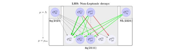
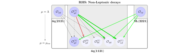
Figure 1: Running of four-fermion operators into operators contributing to $\Delta F=1$ non-leptonic observables. Here the red, green and black lines indicate the operator mixing due to strong, weak and Yukawa couplings respectively. The self-mixing for all couplings is shown by a dashed black line.

Figure 2: Running of four-fermion operators into operators contributing to $\Delta F=2$ observables. Here the red, green and black lines indicate the operator mixing due to strong, weak and Yukawa couplings respectively. The self-mixing for all couplings is shown by a dashed black line.

Figure 3: Running of four-fermion operators into operators contributing to $\Delta F=1$ semi-leptonic observables. Here the red, green and black lines indicate the operator mixing due to strong, weak and Yukawa couplings respectively. The self-mixing for all couplings is shown by a dashed black line.

• At the BSM scale those operators are listed which on the one hand receive a non-vanishing matching contribution and on the other hand imply through RG evolution contributions at the electroweak scale. The latter can come from the same operators with modified Wilson coefficients and from new operators generated through RG evolution. These new operators are placed on a lighter background than the original operators.

• As an example consider the first chart in Fig. 1. The goal is to generate at the electroweak scale four-quark operators contributing to non-leptonic $\Delta S=1$ processes which is indicated by the indices $(2111)$ . The operators

  $${\cal O}_{qq}^{(1)},\qquad{\cal O}_{qu}^{(1)},\qquad{\cal O}_{qd}^{(1)}$$ (42)

  present already at the BSM scale contribute also at the electroweak scale but whereas the indices of the Wilson coefficients ${\cal C}_{qu}^{(1)}$ and ${\cal C}_{qd}^{(1)}$ at the BSM and EW scale are the same, the ones of ${\cal C}_{qq}^{(1)}$ change from $(2121)$ to $(2111)$.

  In addition the operators ${\cal O}_{qu}^{(8)}$ and ${\cal O}_{qd}^{(8)}$ are generated through QCD interactions at the EW scale. Finally the semi-leptonic operator ${\cal O}_{\ell q}^{(1)}$, present already at the BSM scale, while not contributing directly to $\Delta S=1$ non-leptonic observables, can do it indirectly via Wilson coefficients of non-leptonic operators through electroweak interactions.

• The same logic is used in the remaining charts. But one should note that in the RHS the flavour-violating indices are on the right-handed currents so that e.g. on the top of the lower charts in Fig. 1-3 the indices are now $(1121)$ instead of $(2111)$.

• The distinction between strong, weak and Yukawa interactions is made with the help of colours as described in the figure caption.

3.3 $\varepsilon^{\prime}/\varepsilon$

Since $\varepsilon^{\prime}/\varepsilon$ is one of the key observables in our analysis we discuss here explicitly the impact of the LHS and RHS on this observable. The relevant SMEFT matching contributions for $\varepsilon^{\prime}/\varepsilon$ can be found in [68]. Adopting the same short distance basis as therein, namely

$$O_{XAB}^{q} =(\bar{s}^{i}\Gamma_{X}P_{A}d^{i})(\bar{q}^{j}\Gamma_{X}P_{B}q^{j})\,, \widetilde{O}_{XAB}^{q} =(\bar{s}^{i}\Gamma_{X}P_{A}d^{j})(\bar{q}^{j}\Gamma_{X}P_{B}q^{i})\,,$$ (43)

with colour indices $i,j$, chiralities $A,B=L,R$, and Dirac structures $X=S,V,T$ with $\Gamma_{S}=1$, $\Gamma_{V}=\gamma^{\mu}$, $\Gamma_{T}=\sigma^{\mu\nu}$, one finds at the high scale $\Lambda$:

$${\rm(LHS)}: \quad C_{VLR}^{u}=\big{[}{\cal C}_{qu}^{(1)}\big{]}_{2111}\,,\qquad\qquad C_{VLR}^{d}=\big{[}{\cal C}_{qd}^{(1)}\big{]}_{2111}\,,$$ (44)

$${\rm(RHS)}: \quad C_{VRL}^{u}=|V_{ud}|^{2}\big{[}{\cal C}_{qd}^{(1)}\big{]}_{1121}\,,\qquad C_{VRL}^{d}=\big{[}{\cal C}_{qd}^{(1)}\big{]}_{1121}\,,$$ (45)

where we have neglected small contributions. However, as indicated by the red arrows in Fig. 1, the Wilson coefficients $\big{[}{\cal C}_{qu}^{(8)}\big{]}_{2111}$ and $\big{[}{\cal C}_{qd}^{(8)}\big{]}_{2111}$ $(\big{[}{\cal C}_{qd}^{(8)}\big{]}_{1121})$ are induced through QCD running down to the EW scale in the LHS (RHS). At LL one finds [69, 67]:

$$\big{[}{\cal C}_{qu}^{(8)}\big{]}_{2111}(\mu_{\rm EW})=-3\frac{\alpha_{s}}{\pi}\big{[}{\cal C}_{qu}^{(1)}\big{]}_{2111}(\Lambda)\ln{\left(\frac{\mu_{\rm EW}}{\Lambda}\right)}\,,$$ (46)

and similar expressions for $\big{[}{\cal C}_{qd}^{(8)}\big{]}_{2111}$ and $\big{[}{\cal C}_{qd}^{(8)}\big{]}_{1121}$. Therefore, taking QCD RGE effects into account the matching at the BSM scale in (44)-(45) is modified at the EW scale as follows

$${\rm(LHS)}: \quad C_{VLR}^{u}=\big{[}{\cal C}_{qu}^{(1)}\big{]}_{2111}-\frac{1}{6}\big{[}{\cal C}_{qu}^{(8)}\big{]}_{2111}\,,\qquad C_{VLR}^{d}=\big{[}{\cal C}_{qd}^{(1)}\big{]}_{2111}-\frac{1}{6}\big{[}{\cal C}_{qd}^{(8)}\big{]}_{2111}\,,$$ (47)

$$\quad\widetilde{C}_{VLR}^{u}=\frac{1}{2}\big{[}{\cal C}_{qu}^{(8)}\big{]}_{2111}\,,\qquad C_{SRL}^{d}=-\big{[}{\cal C}_{qd}^{(8)}\big{]}_{2111}\,,$$ (48)

$${\rm(RHS)}: \quad C_{VRL}^{u}=|V_{ud}|^{2}\big{(}\big{[}{\cal C}_{qd}^{(1)}\big{]}_{1121}-\frac{1}{6}\big{[}{\cal C}_{qd}^{(8)}\big{]}_{1121}\big{)}\,,\quad C_{VRL}^{d}=\big{[}{\cal C}_{qd}^{(1)}\big{]}_{1121}-\frac{1}{6}\big{[}{\cal C}_{qd}^{(8)}\big{]}_{1121}\,,$$ (49)

$$\quad\widetilde{C}_{VRL}^{u}=\frac{1}{2}|V_{ud}|^{2}\big{[}{\cal C}_{qd}^{(8)}\big{]}_{1121}\,,\qquad C_{SLR}^{d}=-\big{[}{\cal C}_{qd}^{(8)}\big{]}_{1121}\,.$$ (50)

Employing now the master formula for the BSM contribution to $\varepsilon^{\prime}/\varepsilon$ one finds [70, 68, 71]:

$$\left(\frac{\varepsilon^{\prime}}{\varepsilon}\right)_{\rm BSM}\approx -124\cdot{\rm Im}[C_{VLR}^{u}-C_{VRL}^{u}]+117\cdot{\rm Im}[C_{VLR}^{d}-C_{VRL}^{d}]\$$ (51)

$$-430\cdot{\rm Im}[\widetilde{C}_{VLR}^{u}-\widetilde{C}_{VRL}^{u}]+204\cdot{\rm Im}[C_{SLR}^{d}-C_{SRL}^{d}]$$

$$={\rm Im}[-124\big{[}{\cal C}_{qu}^{(1)}\big{]}_{2111}-194.3\big{[}{\cal C}_{qu}^{(8)}\big{]}_{2111}+117\big{[}{\cal C}_{qd}^{(1)}\big{]}_{2111}+184.5\big{[}{\cal C}_{qd}^{(8)}\big{]}_{2111}$$ (52)

$$+(124\big{[}{\cal C}_{qd}^{(1)}\big{]}_{1121}+194.3\big{[}{\cal C}_{qd}^{(8)}\big{]}_{1121})|V_{ud}|^{2}-117\big{[}{\cal C}_{qd}^{(1)}\big{]}_{1121}-184.5\big{[}{\cal C}_{qd}^{(8)}\big{]}_{1121}]\,,$$

where we have used (47)-(50) and the Wilson coefficients on the right-hand side of (51) and (52) are given in units of ($1/\text{TeV}^{2}$). The first and second line in (52) correspond to contributions from the LHS and RHS respectively.

4 $Z^{\prime}$ Contributions: Numerics

In our numerical analysis we investigate the following quantities:

$$R_{\Delta M_{K}} = \frac{\Delta M_{K}^{BSM}}{\Delta M_{K}^{exp}}\,,\quad R_{\nu\bar{\nu}}^{+}=\frac{\mathcal{B}(K^{+}\to\pi^{+}\nu\bar{\nu})}{\mathcal{B}(K^{+}\to\pi^{+}\nu\bar{\nu})_{SM}}\,,\quad R_{\nu\bar{\nu}}^{0}=\frac{\mathcal{B}(K_{L}\to\pi^{0}\nu\bar{\nu})}{\mathcal{B}(K_{L}\to\pi^{0}\nu\bar{\nu})_{SM}}\,,$$ (53)

$$R_{\mu^{+}\mu^{-}}^{S} = \frac{\mathcal{B}(K_{S}\to\mu^{+}\mu^{-})}{\mathcal{B}(K_{S}\to\mu^{+}\mu^{-})_{SM}}\,,\quad R_{\pi\ell^{+}\ell^{-}}^{0}=\frac{\mathcal{B}(K_{L}\to\pi^{0}\ell^{+}\ell^{-})}{\mathcal{B}(K_{L}\to\pi^{0}\ell^{+}\ell^{-})_{SM}}\,.$$

For the numerical analysis the input parameters in Tables 3 and 4 are used. The constraint from $\mathcal{B}(K_{L}\to\mu^{+}\mu^{-})$ at the 2$\sigma$ level is taken into account. The SM predictions for $K^{+}\rightarrow\pi^{+}\nu\bar{\nu}$ and $K_{L}\rightarrow\pi^{0}\nu\bar{\nu}$ are given in (7) and for the remaining decays one finds [27, 72, 73, 74]:

$$\mathcal{B}(K_{S}\to\mu^{+}\mu^{-})_{SM}=(5.2\pm 1.5)\times 10^{-12}\,,\quad\mathcal{B}(K_{L}\to\pi^{0}e^{+}e^{-})_{SM}=3.54^{+0.98}_{-0.85}(1.56^{+0.62}_{-0.49})\times 10^{-11}\,,$$

$$\mathcal{B}(K_{L}\to\pi^{0}\mu^{+}\mu^{-})_{SM}=1.41^{+0.28}_{-0.26}(0.95^{+0.22}_{-0.21})\times 10^{-11}\,,$$ (54)

where for the $K_{L}\to\pi^{0}\ell^{+}\ell^{-}$ decays the numbers in parenthesis denote the destructive interference case. The experimental status of these decays is given by[75, 76, 77]:

$$\mathcal{B}(K_{S}\to\mu^{+}\mu^{-})_{\rm LHCb}<0.8(1.0)\times 10^{-9}\,,\quad\mathcal{B}(K_{L}\to\pi^{0}e^{+}e^{-})_{exp}<28\times 10^{-11}\,,$$

$$\mathcal{B}(K_{L}\to\pi^{0}\mu^{+}\mu^{-})_{exp}<38\times 10^{-11}\,,$$ (55)

Finally, for the LHS and RHS we impose the constraint from $\varepsilon_{K}$ in the following way:

$$\kappa_{\varepsilon}\in[-0.2,0.2]\,,$$ (56)

where $\kappa_{\varepsilon}$ is defined in (12). But we will investigate what happens for a larger range $\kappa_{\varepsilon}\in[-0.5,0.5]$.

$G_{F}=1.16637(1)\times 10^{-5}\,{\rm GeV}^{-2}$	$M_{Z}=91.188(2)\,{\rm GeV}$	$M_{W}=80.385(15)\,{\rm GeV}$
$\sin^{2}\theta_{W}=0.23116(13)$	$\alpha(M_{Z})=1/127.94$	$\alpha_{s}(M_{Z})=0.1184(7)$
$m_{e}=0.511\,{\rm MeV}$	$m_{\mu}=105.66\,{\rm MeV}$	$m_{\tau}=1776.9(1)\,{\rm MeV}$
$m_{u}(2\,{\rm GeV})=2.16(11)\,{\rm MeV}$	$m_{c}(m_{c})=1.279(13)\,{\rm GeV}$	$m_{t}(m_{t})=163(1)\,{\rm GeV}$
$m_{d}(2\,{\rm GeV})=4.68(15)\,{\rm MeV}$	$m_{s}(2\,{\rm GeV})=93.8(24)\,{\rm MeV}$	$m_{b}(m_{b})=4.19^{+0.18}_{-0.06}\,{\rm GeV}$
$m_{K^{\pm}}=493.68(2)\,{\rm MeV}$	$m_{K^{0}}=497.61(1)\,{\rm MeV}$	$\Delta M_{K}=0.5292(9)\times 10^{-2}\,\text{ps}^{-1}$
$m_{B_{d}}=5279.62(15)\,{\rm MeV}$	$m_{B_{s}}=5366.82(22)\,{\rm MeV}$	$|\epsilon_{K}|=2.228(11)\times 10^{-3}$

Table 3: Values of theoretical quantities used for the numerical analysis.

$F_{B_{d}}$ = $190.5(1.3)\,{\rm MeV}$	$F_{B_{s}}$ = $230.7(1.2)\,{\rm MeV}$	$F_{K}=156.1(11)\,{\rm MeV}$
$\hat{B}_{B_{d}}=1.27(10)$	$\hat{B}_{B_{s}}=1.33(6)$	$\hat{B}_{K}=0.766(10)$
$F_{B_{d}}\sqrt{\hat{B}_{B_{d}}}=216(15)\,{\rm MeV}$	$F_{B_{s}}\sqrt{\hat{B}_{B_{s}}}=266(18)\,{\rm MeV}$	$\xi=1.21(2)$
$\eta_{cc}=1.87(76)$	$\eta_{ct}=0.496(47)$	$\eta_{tt}=0.5765(65)$
$\eta_{B}=0.55(1)$	$\phi_{\varepsilon}=43.51(5)^{\circ}$	$\kappa_{\varepsilon}=0.94(2)$
$|V_{us}|=0.2248(8)$	$|V_{ub}|=3.73(14)\times 10^{-3}$	$|V_{cb}|=4.221(78)\times 10^{-2}$

Table 4: Constants used for the numerical analysis.

4.1 Electroweak Penguin Scenario: Left-Handed

We start with a LHS (i.e. $g_{q}^{21}\neq 0$), where the effect in $\varepsilon^{\prime}/\varepsilon$ is achieved through electroweak penguin (EWP) operators such as $Q_{8}$. To generate such operators we choose the quark couplings in the following way:

$$g_{q}^{21}\neq 0\,,\qquad g_{u}^{11}=-2g_{d}^{11}\,,\qquad g_{\ell}^{11,22}\neq 0\qquad\text{(LH-EWP scenario)}\,.$$ (57)

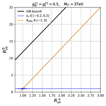
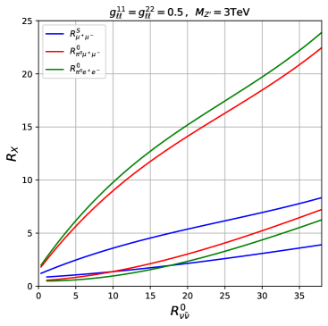
Figure 4: LH-EWP scenario for a $Z^{\prime}$ of $3\,{\rm TeV}$. The correlation between the ratios for the process $K^{+}\to\pi^{+}\nu\bar{\nu}$, $K_{L}\to\pi\nu\bar{\nu}$ defined in (53) is plotted (left). The blue (orange) lines are allowed by $\kappa_{\varepsilon}$ ($\Delta M_{K}$) constraints and the black line represents the GN bound. The correlations between the ratio for $K_{L}\to\pi^{0}\nu\bar{\nu}$ and the ones for $K\to\pi\ell^{+}\ell^{-}$ and $K_{S}\to\mu^{+}\mu^{-}$ are shown (right).

In Fig. 4 (left), we plot the correlation between the ratios for the decays $K^{+}\to\pi^{+}\nu\bar{\nu}$ and $K_{L}\to\pi\nu\bar{\nu}$. Here the horizontal and vertical branches correspond to purely real and imaginary values respectively of the flavour violating coupling $g_{q}^{21}$. Simultaneous presence of both real and imaginary parts, which correspond to the small area at the meeting point of the two branches, are strongly constrained by the allowed range of $\kappa_{\varepsilon}$ (56). Furthermore, requiring the suppression of $\Delta M_{K}$ excludes the horizontal branch, indicating the dominance of the imaginary part over the real part of $g_{q}^{21}$.

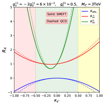
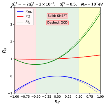
Figure 5: LH-EWP scenario for a $Z^{\prime}$ of $3\,{\rm TeV}$ (left panel) and $10\,{\rm TeV}$ (right panel). The ratios for $\Delta M_{K}$ and for the process $K^{+}\to\pi^{+}\nu\bar{\nu}$, $K_{L}\to\pi\nu\bar{\nu}$ defined in (53) are plotted against $\kappa_{\varepsilon^{\prime}}$. The dashed (solid) lines result from QCD (full SMEFT) running above the EW scale. The yellow, green and red shades correspond to the $\kappa_{\varepsilon^{\prime}}$ scenarios A, B and C as defined in (11).

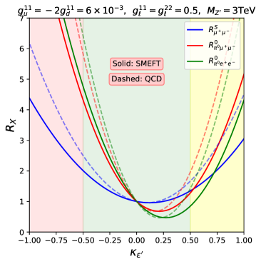
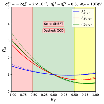
Figure 6: LH-EWP scenario for a $Z^{\prime}$ of $3\,{\rm TeV}$ (left panel) and $10\,{\rm TeV}$ (right panel). The predictions for the ratios of the decays $K_{S}\to\mu^{+}\mu^{-}$, $K_{L}\to\pi^{0}\mu^{+}\mu^{-}$ and $K_{L}\to\pi^{0}e^{+}e^{-}$ defined in eq. (53) are plotted against $\kappa_{\varepsilon^{\prime}}$ . The yellow, green and red shades correspond to the $\kappa_{\varepsilon^{\prime}}$ scenarios A, B and C as defined in (11).

This implies a strong correlation between $K^{+}\to\pi^{+}\nu\bar{\nu}$ and $K_{L}\to\pi\nu\bar{\nu}$ on the MB-branch, so that they can be enhanced or suppressed only simultaneously as shown by the orange colour in this figure. Out of the three $\kappa_{\varepsilon^{\prime}}$ scenarios A, B and C, which are defined in (11), in scenario A, large departures from SM expectations for $K_{L}\rightarrow\pi^{0}\nu\bar{\nu}$ are possible. Similarly, in Fig. 4 (right), the correlations between the ratio for the decay $K_{L}\to\pi\nu\bar{\nu}$ and the ones for $K\to\pi\ell^{+}\ell^{-}$ and $K_{S}\to\mu^{+}\mu^{-}$ are shown. The upper range for $R_{\nu\bar{\nu}}^{0}$ corresponds roughly to the GN bound. If the values from KOTO given in (8) will be confirmed in the future, large departures from the SM predictions for the three rare decays are to be expected. Also the $K^{+}\rightarrow\pi^{+}\nu\bar{\nu}$ branching ratio could be enhanced. Fig. 4 (right) admits two solutions for each decay, corresponding to different values of $\kappa_{\varepsilon^{\prime}}$. The upper branch results from positive values for ${\rm Im}(g_{q}^{21})$ and the lower one from negative ones, since positive (negative) values of ${\rm Im}(g_{q}^{21})$ enhance (reduce) the corresponding ratios.

In Fig. 5 we show the results for the first three different ratios defined in (53) as functions of $\kappa_{\varepsilon^{\prime}}$ for a $Z^{\prime}$ of $3\,{\rm TeV}$ and $10\,{\rm TeV}$ respectively. For the running below the EW scale we use the complete 1-loop QCD and QED running [78, 79] and above the EW scale the full SMEFT RGEs for the solid and only QCD for the dashed lines are used. Clearly, the running is dominated by QCD effects. For $3\,{\rm TeV}$ both $K\rightarrow\pi\nu\bar{\nu}$ branching ratios are enhanced over their SM values, except for a small region around $\kappa_{\varepsilon^{\prime}}\approx 0$. For $10\,{\rm TeV}$, significant BSM effects are only observed for $\kappa_{\varepsilon^{\prime}}\geq 0.5$. $\Delta M_{K}$ is visibly suppressed for sufficiently large $\kappa_{\varepsilon^{\prime}}$. The choice of very small values of $g_{u,d}^{11}$ of $\mathcal{O}(10^{-2})$ is implied, as noticed already in [12], by the desire to suppress $\Delta M_{K}$ in the presence of NP contributions to $\varepsilon^{\prime}/\varepsilon$ in the EWP sector. For $g_{u,d}^{11}$ of $\mathcal{O}(1)$ considered in the latter paper, $\Delta M_{K}$ is enhanced by BSM rather than suppressed which is disfavoured by the present LQCD data. In Fig. 6 we show predictions for the remaining ratios given in (53), where we allow for additional couplings to left-handed electrons ($g_{\ell}^{11}$). We observe that for a lighter $Z^{\prime}$ an enhancement for $R^{0}_{\pi^{0}\mu\mu}$ and $R^{0}_{\pi^{0}ee}$ processes is predicted for negative values of $\kappa_{\varepsilon^{\prime}}$, while for its positive values both suppression as well as enhancement are possible. On the other hand for heavier $Z^{\prime}$ these decay modes are suppressed (enhanced) for positive (negative) values of $\kappa_{\varepsilon^{\prime}}$. The ratio $R_{\mu\mu}^{S}$ is always enhanced. The difference between solid and dashed lines is mainly due to QED RG effects on $\kappa_{\varepsilon^{\prime}}$, generated by semi-leptonic operators.

In Fig. 7 the correlations between $\kappa_{\varepsilon^{\prime}}$ and $R_{\Delta M_{K}}$ and between the ratios for $K^{+}\rightarrow\pi^{+}\nu\bar{\nu}$ and $K_{L}\rightarrow\pi^{0}\nu\bar{\nu}$ and $R_{\Delta M_{K}}$ are shown. As expected, $\kappa_{\varepsilon^{\prime}}$ and $K_{L}\rightarrow\pi^{0}\nu\bar{\nu}$ are much more sensitive to variations of $R_{\Delta M_{K}}$ than it is the case of $K^{+}\rightarrow\pi^{+}\nu\bar{\nu}$.

In Fig. 8 the ratios of Fig. 6 are shown this time as a functions of $R_{\Delta M_{K}}$ for a $Z^{\prime}$ of $3\,{\rm TeV}$ and $10\,{\rm TeV}$. A large enhancement for all processes is possible for both light as well as heavy $Z^{\prime}$, while suppressing $\Delta M_{K}$. The sign of the quark coupling $g_{q}^{21}$ can be fixed by $\kappa_{\varepsilon^{\prime}}$ if the signs of the diagonal quark couplings are known. Similarly the leptonic couplings can be either positive or negative and are not determined by the conditions imposed. The two branches in this figure correspond to different signs of the coupling $g_{q}^{21}$. In any case the hinted $\Delta M_{K}$ anomaly has significant impact on all branching ratios.

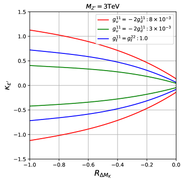
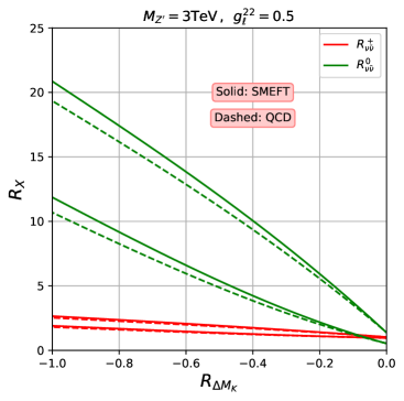
Figure 7: LH-EWP scenario for a $Z^{\prime}$ of $3\,{\rm TeV}$. The $\kappa_{\varepsilon^{\prime}}$ and ratios for the process $K^{+}\to\pi^{+}\nu\bar{\nu}$, $K_{L}\to\pi\nu\bar{\nu}$ (right) defined in (53) are plotted against $R_{\Delta M_{K}}$.

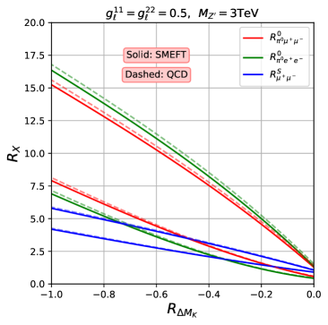
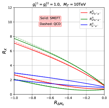
Figure 8: LH-EWP scenario for a $Z^{\prime}$ of $3\,{\rm TeV}$ (left panel) and $10\,{\rm TeV}$ (right panel). The predictions for the ratios of the decays $K_{S}\to\mu^{+}\mu^{-}$, $K_{L}\to\pi^{0}\mu^{+}\mu^{-}$ and $K_{L}\to\pi^{0}e^{+}e^{-}$ defined in (53) are plotted against $R_{\Delta M_{K}}$.

4.2 QCD Penguin Scenario: Left- and Right-Handed

Next we describe the effects related to the required basis rerotation at the electroweak scale, as described in the last point of Sec. 2.3. This has important phenomenological consequences in any scenario, as for example in the QCD penguin (QCDP) scenario, in which a sizable imaginary coupling is present in scenarios A and C for $\kappa_{\varepsilon^{\prime}}$. The LH-QCDP scenario is defined as follows:

$$g_{q}^{21}\neq 0\,,\qquad g_{u}^{11}=g_{d}^{11}\qquad\text{(LH-QCDP scenario)}\,.$$ (58)

Starting with a set of non-zero Wilson coefficients in the down-basis at the high scale $\Lambda$ we evolve them to the EW scale. Along with the Wilson coefficients we also need to evolve the SM parameters including the mass (or Yukawa) matrices as discussed in Section 2.3. But the running of the mass matrices is flavour dependent[66], and consequently after the evolution the mass matrices are not guaranteed to remain in the original basis that we started with. As a result, we need to rotate the mass matrices and hence the Wilson coefficients to adhere to our choice of the down-basis[49]. This issue is discussed in generality in a recent paper [50] but here we confine our discussion focusing on QCDP.

We illustrate this effect and its phenomenological consequences with a concrete example by considering the LH-QCDP scenario studied in the case of significant BSM contributions to $\varepsilon^{\prime}/\varepsilon$ in [12], but now in contrast to that paper including RG SMEFT effects. Considering the LHS, at the high scale $\Lambda$ the operators $[{\cal O}_{qu}^{(1)}]_{2111}$ and $[{\cal O}_{qd}^{(1)}]_{2111}$ are generated. They are then evolved down to the EW scale. But the simultaneous evolution of the mass matrices generates off-diagonal entries in the down-quark Yukawa matrix $Y_{d}$ at the EW scale. This is due to the fact that the running of $Y_{d}$ is proportional to the up-quark Yukawa matrix $Y_{u}$, which is non-diagonal in the down-basis[80]. Indeed, we have

$$16\pi^{2}\frac{dY_{d}}{d\ln{\mu}}\simeq-\frac{3}{2}(Y_{u}{Y_{u}}^{\dagger})Y_{d}+...\,.$$ (59)

To revert to the down-type basis, a rotation of the operators is necessary, as already explained in Section 2.3. Applying this back-rotation to the Wilson coefficients generates $\big{[}{\cal C}_{qd}^{(1)}\big{]}_{2121}$ at the EW scale in the down-basis as:

$$\big{[}{\cal C}_{qd}^{(1)}\big{]}_{2121} = (U^{\dagger}_{d_{L}})_{22}(U_{d_{L}})_{11}(U^{\dagger}_{d_{R}})_{21}(U_{d_{R}})_{11}\big{[}{\cal C}_{qd^{\prime}}^{(1)}\big{]}_{2111}+...\,,$$ (60)

where $\big{[}{\cal C}_{qd^{\prime}}^{(1)}\big{]}_{2111}$ denotes the Wilson coefficient in the RGE basis and the rotation matrices $U_{d_{L}},\,U_{d_{R}}$ satisfy the following equation:

$$M_{d}(\mu_{\rm EW})=U_{d_{L}}^{\dagger}M_{d}^{\prime}(\mu_{\rm EW})U_{d_{R}}\,.$$ (61)

Here the (non-diagonal) down-quark mass matrix $M_{d}^{\prime}$ at the EW scale is obtained by evolving $Y_{d}$ from the high scale $\Lambda$ down to $\mu_{\rm EW}$. In the LL approximation we have:

$$M_{d}^{\prime}(\mu_{\rm EW})=M_{d}(\Lambda)+\frac{v}{\sqrt{2}}\frac{\beta_{Y_{d}}(\Lambda)}{16\pi^{2}}\ln{\left(\frac{\mu_{\rm EW}}{\Lambda}\right)}\,.$$ (62)

However, the Wilson coefficient $\big{[}{\cal C}_{qd}^{(1)}\big{]}_{2121}$ is strongly constrained by $\varepsilon_{K}$ due to the large hadronic matrix element multiplying it.

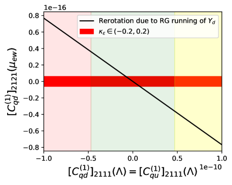
Figure 9: LH-QCDP scenario, where the operator $[{\cal O}_{qd}^{(1)}]_{2121}$ is generated after RGE running of $Y_{d}$ and back-rotation to the down-basis at the EW scale. The allowed regions for the Wilson coefficients are in red for $\varepsilon_{K}$, and vertical bands represent the three $\varepsilon^{\prime}/\varepsilon$ scenarios.

This scenario is illustrated in Fig. 9, where at the high scale we vary the input values of the Wilson coefficients $\big{[}{\cal C}_{qd}^{(1)}\big{]}_{2111}$ and $\big{[}{\cal C}_{qu}^{(1)}\big{]}_{2111}$ as shown on the x-axis. On the y-axis we show the output value of the Wilson coefficient $\big{[}{\cal C}_{qd}^{(1)}\big{]}_{2121}$ at the EW scale which is generated through the back-rotation of (60). However, this LR operator gives a large contribution to $\varepsilon_{K}$[12]

$$\kappa_{\varepsilon}\simeq 3.1\times 10^{16}\times{\rm Im}\left(\big{[}{\cal C}_{qd}^{(1)}\big{]}_{2121}(\mu_{ew}){\rm GeV^{-2}}\right).$$ (63)

The allowed values for the Wilson coefficients of the three mentioned operators are shown in the red region, given the constraints from $\varepsilon_{K}$. This shows that in the LHS with QCDP dominance, significant BSM contributions to $\varepsilon^{\prime}/\varepsilon$ imply a large contribution to $\varepsilon_{K}$ inevitably generated by the running of Yukawas and subsequent back-rotation of the Wilson coefficients at the EW scale. Consequently, the QCDP scenario for $\varepsilon^{\prime}/\varepsilon$, considered in [12] is ruled out, since in this case significant BSM contributions to $\varepsilon^{\prime}/\varepsilon$ would be required to fit the data. Similar comments apply to the RHS scenario defined by

$$g_{q}^{11}\neq 0\,,\qquad g_{d}^{21}\neq 0\,.\qquad\text{(RH-QCDP scenario)}$$ (64)

In this case only the QCDP scenario can be constructed. Due to $SU(2)_{L}$ gauge invariance the coefficient of the so-called $Q_{8}^{\prime}$ operator, which otherwise would give a leading contribution to $\varepsilon^{\prime}/\varepsilon$, vanishes.

On the other hand, in the case of the EWP dominance i.e $\big{[}{\cal C}_{qd}^{(1)}\big{]}_{2111}=-\frac{1}{2}\big{[}{\cal C}_{qu}^{(1)}\big{]}_{2111}$, also considered in [12], this effect is negligible. This is simply because in this case a much smaller value of $\big{[}{\cal C}_{qd}^{(1)}\big{]}_{2111}$ is needed to enhance sufficiently $\varepsilon^{\prime}/\varepsilon$.

4.3 Left-Right Scenario

We have just seen that in the LHS there was a very strong correlation between $K^{+}\rightarrow\pi^{+}\nu\bar{\nu}$ and $K_{L}\rightarrow\pi^{0}\nu\bar{\nu}$ branching ratios on the MB-branch. As explained in [22] this strict correlation originates in the same complex phase present in NP contributions to $\varepsilon_{K}$ and rare Kaon decays in question provided NP contributions to $\varepsilon_{K}$ are small. This is in fact evident in our case because the same $Z^{\prime}\bar{s}d$ coupling enters both $K^{+}\rightarrow\pi^{+}\nu\bar{\nu}$ and $K_{L}\rightarrow\pi^{0}\nu\bar{\nu}$ and $\varepsilon_{K}$.

Now,

$$(\varepsilon_{K})_{\text{BSM}}\propto\left[(\rm{Re}(g_{sd})(\rm{Im}(g_{sd})\right],$$ (65)

and to make sure that this contribution is small either $\rm{Re}(g_{sd})$ or $\rm{Im}(g_{sd})$ must be small. If $\rm{Im}(g_{sd})$ is small the horizontal line in Fig. 4 results with NP basically only in $K^{+}\rightarrow\pi^{+}\nu\bar{\nu}$. If $\rm{Re}(g_{sd})$ is small then there are NP contributions to both $K_{L}\rightarrow\pi^{0}\nu\bar{\nu}$ and $K^{+}\rightarrow\pi^{+}\nu\bar{\nu}$ correlated on the MB-branch. In our case this second solution is chosen by the desire to explain the $\Delta M_{K}$ anomaly. However, such a correlation precludes the pattern of simultaneously enhancing $K_{L}\rightarrow\pi^{0}\nu\bar{\nu}$ and suppressing $K^{+}\rightarrow\pi^{+}\nu\bar{\nu}$ possibly hinted by the NA62 and KOTO results.

It is known from various studies that such a pattern can be obtained through the introduction of new operators and the most effective in this respect are scenarios in which both left-handed and right-handed flavour-violating NP couplings are present, breaking the correlation between $K^{0}-\bar{K}^{0}$ mixing and rare Kaon decays and thereby eliminating the impact of the $\varepsilon_{K}$ constraint on rare Kaon decays. The presence of left-right operators requires some fine-tuning of the parameters in order to satisfy the $\varepsilon_{K}$ constraint but such operators do not contribute to rare decays and the presence of new parameters does not affect directly these decays. Examples of such scenarios are $Z^{\prime}$ models with LH and RH couplings considered in [59] and the earlier studies in the context of the general MSSM [81, 82, 83, 84, 85] and Randall-Sundrum models [86, 87]. See in particular Fig. 6 in [86] and Fig 7 in [59]. Needless to say also the correlations between NP contributions to $\Delta M_{K}$ and rare decays are diluted, although the necessity of non-vanishing complex couplings required by the hinted $\Delta M_{K}$ anomaly will certainly have some impact on rare Kaon decays.

The Left-Right (LR) scenario at $3\,{\rm TeV}$ is defined by

$$g_{q}^{21},g_{d}^{21}\neq 0\,,\qquad g_{u}^{11}=-2g_{d}^{11}\,,\qquad\text{(LR-EWP scenario)}$$ (66)

which is equivalent to the LH-EWP scenario without imposing $\Delta F=2$ constraints[59].

In Fig. 10 correlations between ratios for $K_{L}\rightarrow\pi^{0}\nu\bar{\nu}$ and $K^{+}\rightarrow\pi^{+}\nu\bar{\nu}$ as in (53) are considered. Clearly no strong correlation is observed when both LH and RH couplings are allowed as shown in the green region. Similarly, the strong correlation between $K^{+}\rightarrow\pi^{+}\nu\bar{\nu}$ and $\kappa_{\varepsilon^{\prime}}$ observed in the LH-EWP scenario is absent in the LR scenario because $R^{+}_{\nu\bar{\nu}}$ also depends on the real part, which is not fixed through $\varepsilon^{\prime}/\varepsilon$.

Imposing however the constraint from $\varepsilon_{K}$ and therefore studying a LH-EWP scenario limits the allowed parameter space drastically. Furthermore, as shown in Sec. 4.1 out of the two branches in the $R^{+}_{\nu\bar{\nu}}$-$R^{0}_{\nu\bar{\nu}}$ plane allowed by $\varepsilon_{K}$, the horizontal branch shown in blue is disfavored by the requirement of suppression of $\Delta M_{K}$. In the red area we show the allowed region for the LH-EWP scenario with $\varepsilon_{K}\in[-0.5,0.5]$.

Importantly, as evident from Fig. 10, the simultaneous enhancement of $K_{L}\rightarrow\pi^{0}\nu\bar{\nu}$ and suppression of $K^{+}\rightarrow\pi^{+}\nu\bar{\nu}$ branching ratios is only possible in the presence of both LH and RH flavour-violating couplings. Also, the observables $R_{\nu\bar{\nu}}^{0}$ and $\kappa_{\varepsilon^{\prime}}$ only depend on the imaginary part of the flavour violating coupling. Therefore they are strongly correlated in the LR as well as in the LHS scenario.

This agrees with the findings in [33], in which only QCD has been considered. The correlation between $R^{+}_{\nu\bar{\nu}}$ and $R^{0}_{\nu\bar{\nu}}$ in this setup is therefore invariant under Yukawa running effects.

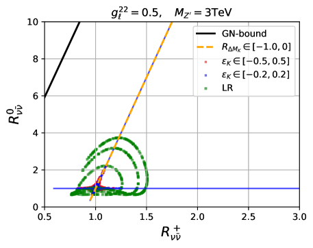
Figure 10: The ratios for $K^{+}\to\pi^{+}\nu\bar{\nu}$ and $K_{L}\to\pi\nu\bar{\nu}$ defined in (53) are plotted. The LR scenario shown in green and LH-EWP scenario in blue and red with $\varepsilon_{K}\in[-0.2,0.2]$ and $[-0.5,0.5]$ respectively for a $Z^{\prime}$ of $3\,{\rm TeV}$. The orange line also satisfies $R_{\Delta M_{K}}\in[-1.0,0]$. The GN bound is shown in black.

5 $Z$ Contributions: Numerics

	$\psi^{2}H^{2}D$
${\cal O}_{H\ell}^{(1)}$	$(H^{\dagger}i\overleftrightarrow{D}_{\!\!\mu}H)(\bar{\ell}^{i}\gamma^{\mu}\ell^{j})$
${\cal O}_{H\ell}^{(3)}$	$(H^{\dagger}i\overleftrightarrow{D}^{I}_{\!\!\mu}H)(\bar{\ell}^{i}\tau^{I}\gamma^{\mu}\ell^{j})$
${\cal O}_{He}$	$(H^{\dagger}i\overleftrightarrow{D}_{\!\!\mu}H)(\bar{e}^{i}\gamma^{\mu}e^{j})$
${\cal O}_{Hq}^{(1)}$	$(H^{\dagger}i\overleftrightarrow{D}_{\!\!\mu}H)(\bar{q}^{i}\gamma^{\mu}q^{j})$
${\cal O}_{Hq}^{(3)}$	$(H^{\dagger}i\overleftrightarrow{D}^{I}_{\!\!\mu}H)(\bar{q}^{i}\tau^{I}\gamma^{\mu}q^{j})$
${\cal O}_{Hu}$	$(H^{\dagger}i\overleftrightarrow{D}_{\!\!\mu}H)(\bar{u}^{i}\gamma^{\mu}u^{j})$
${\cal O}_{Hd}$	$(H^{\dagger}i\overleftrightarrow{D}_{\!\!\mu}H)(\bar{d}^{i}\gamma^{\mu}d^{j})$
${\cal O}_{Hud}$	$(\widetilde{H}^{\dagger}i{D}_{\!\mu}H)(\bar{u}^{i}\gamma^{\mu}d^{j})$

Table 5: Dimension-six $\psi^{2}H^{2}D$ operators in SMEFT.

5.1 Preliminaries

In this section we consider flavour violating (FV) $Z$ couplings induced by FV $Z^{\prime}$ couplings through SMEFT RG running effects. Let us consider the LL running from the BSM scale $\Lambda$ to the EW scale $\mu_{\text{EW}}$. For the Wilson coefficients of the $\psi^{2}H^{2}D$ operators defined in Tab. 5 keeping only the top Yukawa coupling $y_{t}$ and neglecting the terms of $\mathcal{O}(V_{ts}^{2})$ and $\mathcal{O}({V_{tb}V_{ts}})$ one finds [69, 66]

$$\big{[}{\cal C}_{Hq}^{(1)}\big{]}_{ij}(\mu_{\rm EW}) =\frac{y_{t}^{2}}{8\pi^{2}}\left(\big{[}{\cal C}_{qq}^{(1)}\big{]}_{3ji3}(\Lambda)+2N_{c}\big{[}{\cal C}_{qq}^{(1)}\big{]}_{33ij}(\Lambda)-N_{c}\big{[}{\cal C}_{qu}^{(1)}\big{]}_{ij33}(\Lambda)\right)\ln{\left(\frac{\mu_{\text{EW}}}{\Lambda}\right)}\,,$$ (67)

$$\big{[}{\cal C}_{Hq}^{(3)}\big{]}_{ij}(\mu_{\rm EW}) =-\frac{y_{t}^{2}}{8\pi^{2}}\big{[}{\cal C}_{qq}^{(1)}\big{]}_{i33j}(\Lambda)\ln{\left(\frac{\mu_{\text{EW}}}{\Lambda}\right)}\,,$$ (68)

$$\big{[}{\cal C}_{Hd}\big{]}_{ij}(\mu_{\rm EW}) =\frac{N_{c}y_{t}^{2}}{8\pi^{2}}\left(\big{[}{\cal C}_{qd}^{(1)}\big{]}_{33ij}(\Lambda)-\big{[}{\cal C}_{ud}^{(1)}\big{]}_{33ij}(\Lambda)\right)\ln{\left(\frac{\mu_{\text{EW}}}{\Lambda}\right)}\,,$$ (69)

$$\big{[}{\cal C}_{Hu}\big{]}_{ij}(\mu_{\rm EW}) =\frac{y_{t}^{2}}{8\pi^{2}}\left(N_{c}\big{[}{\cal C}_{qu}^{(1)}\big{]}_{33ij}(\Lambda)-2N_{c}\big{[}{\cal C}_{uu}\big{]}_{ij33}(\Lambda)-2\big{[}{\cal C}_{uu}\big{]}_{i33j}(\Lambda)\right)\ln{\left(\frac{\mu_{\text{EW}}}{\Lambda}\right)}\,,$$ (70)

$$\big{[}{\cal C}_{H\ell}^{(1)}\big{]}_{ij}(\mu_{\rm EW}) =\frac{N_{c}y_{t}^{2}}{8\pi^{2}}\left(\big{[}{\cal C}_{\ell q}^{(1)}\big{]}_{ij33}(\Lambda)-\big{[}{\cal C}_{\ell u}\big{]}_{ij33}(\Lambda)\right)\ln{\left(\frac{\mu_{\text{EW}}}{\Lambda}\right)}\,,$$ (71)

$$\big{[}{\cal C}_{He}\big{]}_{ij}(\mu_{\rm EW}) =-\frac{N_{c}y_{t}^{2}}{8\pi^{2}}\left(\big{[}{\cal C}_{eu}\big{]}_{ij33}(\Lambda)-\big{[}{\cal C}_{qe}\big{]}_{33ij}(\Lambda)\right)\ln{\left(\frac{\mu_{\text{EW}}}{\Lambda}\right)}\,,$$ (72)

whereas ${\cal O}_{H\ell}^{(3)}$ and ${\cal O}_{Hud}$ are not generated in this approximation. Yukawa running effects therefore generate modified $Z$-couplings to the SM fermions.

We can now express the usual FC quark couplings of the $Z$ in terms of ${\cal C}_{Hq}^{(1,3)}$, ${\cal C}_{Hu}$ and ${\cal C}_{Hd}$. We have first

$$\mathcal{L}_{\bar{\psi}\psi Z}^{\rm BSM} =Z_{\mu}\sum_{\psi=u,d}\bar{\psi}_{i}\,\gamma^{\mu}\left([\Delta_{L}^{\psi}(Z)]_{ij}\,P_{L}\,+\,[\Delta_{R}^{\psi}(Z)]_{ij}\,P_{R}\right)\psi_{j}\,,$$ (73)

with $\psi=u,d$ distinguishing between $up$- and $down$-quark couplings. These complex-valued couplings are related to the SMEFT Wilson coefficients through [37]

$$\phantom{x}[\Delta^{u}_{L}(Z)]_{ij} =-\frac{g_{Z}}{2}v^{2}\left[{\cal C}_{Hq}^{(1)}-{\cal C}_{Hq}^{(3)}\right]_{ij},\qquad [\Delta^{u}_{R}(Z)]_{ij} =-\frac{g_{Z}}{2}v^{2}\big{[}{\cal C}_{Hu}\big{]}_{ij}\,,$$ (74)

$$[\Delta^{d}_{L}(Z)]_{ij} =-\frac{g_{Z}}{2}v^{2}\left[{\cal C}_{Hq}^{(1)}+{\cal C}_{Hq}^{(3)}\right]_{ij},\qquad [\Delta^{d}_{R}(Z)]_{ij} =-\frac{g_{Z}}{2}v^{2}\big{[}{\cal C}_{Hd}\big{]}_{ij}\,,$$

where $g_{Z}=\sqrt{g_{1}^{2}+g_{2}^{2}}$ and $v=246\,{\rm GeV}$ is the electroweak vacuum expectation value.

In the $Z^{\prime}$ scenario considered here the $\psi^{2}H^{2}D$ operators are generated through RG effects and are smaller than in the case where these operators are already present at the high scale [37, 38, 46]. For the time being we assume that this is not the case here but we will comment briefly on their possible impact on our analysis below.

5.2 Impact of RG-Induced $Z$ on LH-EWP Scenario

In this subsection we study an explicit example of FV $Z$ couplings induced by FV $Z^{\prime}$ couplings through SMEFT RG running effects and its effect on the ratios in (53). For this purpose we assume two scenarios: In the first one only direct contributions from a $Z^{\prime}$ are generated at the matching scale. This corresponds to the LH-EWP setup in Subsection 4.1. In the second one we allow for additional non-zero couplings to the third generation quarks. The up-type quark coupling will then generate through (67) modified $Z$-couplings, which induce an additional effect compared to the $Z^{\prime}$-only case. We choose the various couplings at the matching scale as follows:

$$Z^{\prime} : g_{q}^{21}\neq 0\,\,\ g_{u}^{11}=-2g_{d}^{11}\neq 0,\,\ g_{\ell}^{22}\neq 0,$$ (75)

$$Z^{\prime}+Z : \,\ Z^{\prime}\,\ +\,\ g_{u}^{33}=-2g_{d}^{33}\neq 0.$$ (76)

In the $Z^{\prime}+Z$ case non-zero values of the couplings $g_{q}^{21}$ and $g_{u}^{33}$ lead to the flavour violating coupling of the $Z$-boson (74)

$$[\Delta_{L}^{d}(Z)]_{21}=g_{Z}\frac{y_{t}^{2}N_{c}}{16\pi^{2}}v^{2}\big{[}{\cal C}_{qu}^{(1)}\big{]}_{2133}\ln{\left(\frac{\mu_{\rm EW}}{\Lambda}\right)}.$$ (77)

Since the usual SM $Z$ couplings obey the relation

$$[\Delta_{R}^{u}(Z)]_{11}=-2[\Delta_{R}^{d}(Z)]_{11}\,,$$ (78)

the operators $Q_{7}$ and $Q_{8}$ are generated through matching and QCD running, respectively. The $Z$ contributions to $\varepsilon^{\prime}/\varepsilon$ generated from a $Z^{\prime}$ via RGE running are therefore of the EWP type.

The results for the above two scenarios are shown in Fig. 11, where for a $Z^{\prime}$ of 3$\,{\rm TeV}$ the same values for the couplings as in Fig. 5 are assumed. In addition we have

$$g_{u}^{33}=-2g_{d}^{33}=0.1\,,$$ (79)

for the $Z^{\prime}+Z$ case. The dashed and solid lines correspond to the $Z^{\prime}$ and $Z^{\prime}+Z$ case respectively. The additional contributions due to the modified $Z$-couplings are destructive to $\kappa_{\varepsilon^{\prime}}$ in this setup, so that a larger value of $g_{q}^{21}$ is needed in order to obtain the same value of $\kappa_{\varepsilon^{\prime}}$ in the presence of $Z$ contributions. Therefore, for a given value of $\kappa_{\varepsilon^{\prime}}$ the effect in semi-leptonic decays and $\Delta M_{K}$ is enhanced as compared to the $Z^{\prime}$-solo scenario. By changing the sign of the third-generation couplings, a constructive effect can be achieved for $\kappa_{\varepsilon^{\prime}}$.

In the left chart of Figure 11 $R^{0}_{\nu\bar{\nu}}$ and $R^{+}_{\nu\bar{\nu}}$ are enhanced whereas $\Delta M_{K}$ is suppressed. The modified $Z$ contributions can have large influence on $K_{L}\to\pi^{0}\nu\bar{\nu}$ which is less pronounced for $K^{+}\to\pi^{+}\nu\bar{\nu}$ for moderate values of $\varepsilon^{\prime}/\varepsilon$. The effect in $\Delta M_{K}$ is also less pronounced since the modified $Z$ coupling enters quadratically. For the predictions of the (semi)-leptonic decays in the right chart in Figure 11 the effect of the generated FV $Z$ coupling is significant for larger absolute values of $\kappa_{\varepsilon^{\prime}}$ and predicts enhancements of all considered ratios.

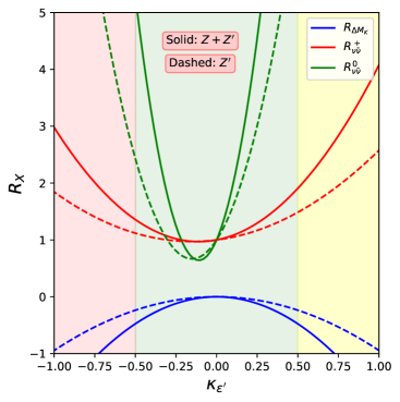
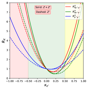
Figure 11: This figure shows how the $Z$-contributions to $\varepsilon^{\prime}/\varepsilon$ and other Kaon observables are generated from a $Z^{\prime}$ through RG running.

5.3 $\varepsilon^{\prime}/\varepsilon$ and Rare decays from RG-Induced $Z$

In our previous discussion we found that in order to have significant BSM contributions to $\varepsilon^{\prime}/\varepsilon$ within the EWP scenario right-handed flavour diagonal couplings to the first generation quarks are required. However, in this subsection we show that one can also get BSM contributions to $\varepsilon^{\prime}/\varepsilon$ even from purely left-handed $Z^{\prime}$ couplings. This can happen through top-Yukawa RG running effects. For this purpose we assume a scenario in which at the high scale the diagonal couplings to the first generation quarks vanish and allow for a rather large third generation coupling, namely

$$g_{q}^{21}\neq 0\,,\quad g_{u}^{11}=g_{d}^{11}=0\,,\quad g_{q}^{33}=0.5\,.$$ (80)

This choice ensures vanishing of the direct $Z^{\prime}$ contribution to $\varepsilon^{\prime}/\varepsilon$ through EWPs. In this setup the Wilson coefficient $\big{[}{\cal C}_{qq}^{(1)}\big{]}_{2133}$ is generated at the BSM scale, which in turn generates $\big{[}{\cal C}_{Hq}^{(1)}\big{]}_{21}$ at the EW scale through top-Yukawa RGEs, as shown in (67). This leads to the flavour violating coupling of the $Z$-boson (74)

$$[\Delta_{L}^{d}(Z)]_{21}=-g_{Z}\frac{y_{t}^{2}N_{c}}{8\pi^{2}}v^{2}\big{[}{\cal C}_{qq}^{(1)}\big{]}_{2133}\ln{\left(\frac{\mu_{\rm EW}}{\Lambda}\right)}\,,$$ (81)

which along with the usual SM $Z$ couplings (78), generate the operators $Q_{7}$ and $Q_{8}$. This effect is displayed in Figure 12. The different ratios of (53) are shown as a function of $\kappa_{\varepsilon^{\prime}}$. A strong suppression of $\Delta M_{K}$ and correlation with $\varepsilon^{\prime}/\varepsilon$ is possible. The large effect in $\Delta M_{K}$ is simply due to the sizable value of the flavour violating coupling present at the BSM scale. Except for $R_{\nu\bar{\nu}}^{0}$ all other ratios are almost at their SM values and do not depend on $\kappa_{\varepsilon^{\prime}}$. In LHS or RHS $R^{0}_{\nu\bar{\nu}}$ goes down (up) with increased (decreased) $\kappa_{\varepsilon^{\prime}}$ in $Z$-scenarios. This is because of special values of flavour diagonal $Zq\bar{q}$ couplings that equal the SM ones in this scenario. See the plots in [33, 12].

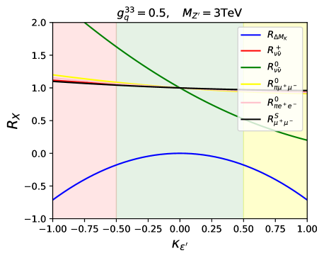
Figure 12: This figure shows how the $Z$-contributions to $\varepsilon^{\prime}/\varepsilon$ and other Kaon observables are generated from a $Z^{\prime}$ with purely left-handed quark couplings through RG running.

In a similar fashion with different combinations of $Z^{\prime}$ couplings at the NP scale the $Z$ couplings can be modified through other $\psi^{2}H^{2}D^{2}$ operators given in (67)-(72).

Finally, it should be emphasized following [37, 38] that $Z$ contributions to $\varepsilon_{K}$ and $\Delta M_{K}$ considered by us correspond really to dimension-eight operators, but the fact that the FV $Z$ couplings in rare decays and Wilson coefficients of these operators are the same implies correlations between $\Delta S=1$ and $\Delta S=2$ observables [40]. These correlations are strongly modified, even broken, in the presence of non-vanishing Wilson coefficients of $\psi^{2}H^{2}D$ operators already at the NP scale. Indeed, through top-Yukawa RG effects dimension-six operators contributing to $\varepsilon_{K}$ and $\Delta M_{K}$ are generated, implying in particular in the case of the ${\cal O}_{Hd}$ operator strong constraints on rare Kaon decays [27, 37, 38].

6 Summary and Outlook

The main goal of our paper was to confront $Z^{\prime}$ scenarios with the pattern of BSM contributions hinted by recent results on $\varepsilon^{\prime}/\varepsilon$, $\Delta M_{K}$, $K^{+}\rightarrow\pi^{+}\nu\bar{\nu}$ and $K_{L}\rightarrow\pi^{0}\nu\bar{\nu}$ that appear to

• allow significant positive or negative BSM contributions to $\varepsilon^{\prime}/\varepsilon$ relative to its SM value,

• suppress the mass difference $\Delta M_{K}$ relative to the recent SM value obtained by the RBC-UKQCD collaboration,

• suppress the branching ratio for $K^{+}\rightarrow\pi^{+}\nu\bar{\nu}$ relative to the precise SM predictions as indicated by the recent result from the NA62 collaboration, although significant enhancements are still possible,

• enhance the branching ratio for $K_{L}\rightarrow\pi^{0}\nu\bar{\nu}$ relative to the precise SM prediction as hinted by the recent result from the KOTO collaboration.

Taking into account the constraints from $\varepsilon_{K}$ and $K_{L}\to\mu^{+}\mu^{-}$ we have calculated $\Delta M_{K}$ and the branching ratios for $K^{+}\rightarrow\pi^{+}\nu\bar{\nu}$ and $K_{L}\rightarrow\pi^{0}\nu\bar{\nu}$ as functions of the parameter $\kappa_{\varepsilon^{\prime}}$ introduced in [12] for the choices of $Z^{\prime}$ couplings to quarks and leptons that can reproduce the pattern of deviations from SM expectations summarized above. For these choices of couplings we have calculated the implications for $K_{S}\to\mu^{+}\mu^{-}$ and $K_{L}\to\pi^{0}\ell^{+}\ell^{-}$ again as functions of $\kappa_{\varepsilon^{\prime}}$. Moreover, we have investigated correlations between all these observables in various $Z^{\prime}$ scenarios.

While an analysis of this sort has been already presented in [12], prior to the last three hints for the pattern of BSM contributions, and earlier analyses can be found in [40, 41], this is the first analysis of this set of observables to date that took into account RG effects in the framework of the SMEFT, in particular the effects of top Yukawa couplings.

In this context we have also investigated for the first time whether the presence of a heavy $Z^{\prime}$ with flavour violating couplings could generate through top Yukawa renormalization group effects FCNCs mediated by the SM $Z$-boson. Our results can be found in numerous plots. Here we want to list the most important lessons from our analysis.

Lesson 1: While the correlation between the enhancement of $\varepsilon^{\prime}/\varepsilon$ with the suppression of $\Delta M_{K}$ has been already pointed out in the context of the QCD penguin scenario for $\varepsilon^{\prime}/\varepsilon$ for flavour diagonal $Z^{\prime}$ couplings to quarks of $\mathcal{O}(1)$ in [12], we find that the inclusion of RG top quark Yukawa effects rules out this scenario through the $\varepsilon_{K}$ constraint.

Lesson 2: While, as noticed already in [12], the suppression of $\Delta M_{K}$ in the presence of the enhancement of $\varepsilon^{\prime}/\varepsilon$ could in the EW penguin scenario be only obtained for flavour diagonal $Z^{\prime}$ couplings to quarks of $\mathcal{O}(10^{-2})$, a numerical analysis of such a scenario has not been presented there. Our analysis demonstrates that the expectations from [12] are confirmed in the presence of the full RG SMEFT analysis. In particular the $\varepsilon_{K}$ constraints are satisfied.

Lesson 3: We point out that the present pattern of possible BSM effects in $K^{+}\rightarrow\pi^{+}\nu\bar{\nu}$ and $K_{L}\rightarrow\pi^{0}\nu\bar{\nu}$ gives in the context of $Z^{\prime}$ models some indication for the presence of right-handed flavour violating currents at work. The confirmation of these findings requires in particular a much more accurate measurement of the $K^{+}\rightarrow\pi^{+}\nu\bar{\nu}$ branching ratio by NA62. Otherwise a strong correlation between $K^{+}\rightarrow\pi^{+}\nu\bar{\nu}$ and $K_{L}\rightarrow\pi^{0}\nu\bar{\nu}$ branching ratios on the MB-branch is implied by the hinted $\Delta M_{K}$ anomaly. In this case if the large enhancement of $K_{L}\rightarrow\pi^{0}\nu\bar{\nu}$ branching ratios signaled by the KOTO experiment is confirmed one day, also significant enhancement of the $K^{+}\rightarrow\pi^{+}\nu\bar{\nu}$ branching ratio over its SM value is to be expected. As seen in Fig. 4, even larger departures from SM predictions should then be observed in $K\to\pi\ell^{+}\ell^{-}$ and $K_{S}\to\mu^{+}\mu^{-}$.

Lesson 4: We have demonstrated that RG effects can in the presence of $Z^{\prime}$ contributions generate flavour-violating $Z$ contributions to $\varepsilon^{\prime}/\varepsilon$ and rare decays that have significant impact on the phenomenology as shown in Fig. 11. What we also find is that in the presence of $\mathcal{O}(1)$ diagonal $Z^{\prime}$ top-quark couplings, the $(V-A)\times(V+A)$ EWP operators can be generated solely through the RG induced flavour-violating $Z$ couplings. As shown in Fig. 12 this effect is sufficiently strong to provide significant BSM contributions to $\varepsilon^{\prime}/\varepsilon$, if required, while simultaneously suppressing $\Delta M_{K}$.

Lesson 5: The impact of BSM effects on rare Kaon decays depends both on the scenarios discussed and on the values of the couplings involved. With improved measurements it will be possibly to select the favorite scenarios. In this context the determination of the parameter $\kappa_{\varepsilon^{\prime}}$ through improved LQCD calculations will be important because, as seen in several plots, some of the rare branching ratios depend sensitively on this parameter.

We are looking forward to experimental and theoretical developments in the coming years. Our plots will allow to monitor them and help to identify the successful $Z^{\prime}$ scenarios.

Appendix A Hadronic matrix elements

In this appendix we report the hadronic matrix elements we use for the numerics of $\varepsilon^{\prime}/\varepsilon$, which have been updated recently by the RBC-UKQCD collaboration [13]. They are given in Tab. 6.

$Q_{i}$	$\langle Q_{i}\rangle_{0}$	$\langle Q_{i}\rangle_{2}$
$Q_{3}$	$-0.075(57)(12)$	$\mathrm{𝟎}$
$Q_{4}$	$0.093(51)(15)$	$\mathrm{𝟎}$
$Q_{5}$	$-0.120(53)(19)$	$\mathrm{𝟎}$
$Q_{6}$	$-0.641(46)(101)$	$\mathrm{𝟎}$
$Q_{7}$	$0.217(16)(34)$	$0.0989(68)(30)$
$Q_{8}$	$1.583(30)(249)$	$0.683(19)(41)$
$Q_{9}$	$-0.059(17)(9)$	$0.0128(3)(8)$

Table 6: Numerical values of $K\to\pi\pi$ SM hadronic matrix elements used in our analysis.

References

- [1] A. J. Buras and J. Girrbach, Towards the Identification of New Physics through Quark Flavour Violating Processes, Rept. Prog. Phys. 77 (2014) 086201, [arXiv:1306.3775].
- [2] M. Gaillard and B. W. Lee, Rare Decay Modes of the K-Mesons in Gauge Theories, Phys. Rev. D10 (1974) 897.
- [3] Z. Bai, N. H. Christ, T. Izubuchi, C. T. Sachrajda, A. Soni, and J. Yu, Mass Difference from Lattice QCD, Phys. Rev. Lett. 113 (2014) 112003, [arXiv:1406.0916].
- [4] N. H. Christ, X. Feng, G. Martinelli, and C. T. Sachrajda, Effects of finite volume on the - mass difference, Phys. Rev. D91 (2015), no. 11 114510, [arXiv:1504.01170].
- [5] Z. Bai, N. H. Christ, and C. T. Sachrajda, The - Mass Difference, EPJ Web Conf. 175 (2018) 13017.
- [6] J. Gérard, W. Grimus, A. Raychaudhuri, and G. Zoupanos, Super Kobayashi-Maskawa CP Violation, Phys. Lett. B 140 (1984) 349–356.
- [7] F. Gabbiani, E. Gabrielli, A. Masiero, and L. Silvestrini, A Complete analysis of FCNC and CP constraints in general SUSY extensions of the standard model, Nucl. Phys. B 477 (1996) 321–352, [hep-ph/9604387].
- [8] UTfit Collaboration, M. Bona et al., Model-independent constraints on F=2 operators and the scale of new physics, JHEP 0803 (2008) 049, [arXiv:0707.0636]. Updates available on http://www.utfit.org.
- [9] G. Isidori, Y. Nir, and G. Perez, Flavor Physics Constraints for Physics Beyond the Standard Model, Ann.Rev.Nucl.Part.Sci. 60 (2010) 355, [arXiv:1002.0900].
- [10] L. Silvestrini and M. Valli, Model-independent Bounds on the Standard Model Effective Theory from Flavour Physics, Phys. Lett. B 799 (2019) 135062, [arXiv:1812.10913].
- [11] L. Calibbi, A. Crivellin, F. Kirk, C. A. Manzari, and L. Vernazza, models with less-minimal flavour violation, Phys. Rev. D 101 (2020), no. 9 095003, [arXiv:1910.00014].
- [12] A. J. Buras, New physics patterns in and with implications for rare kaon decays and , JHEP 04 (2016) 071, [arXiv:1601.00005].
- [13] R. Abbott et al., Direct CP violation and the rule in decay from the Standard Model, arXiv:2004.09440.
- [14] J. Aebischer, C. Bobeth, and A. J. Buras, On the importance of NNLO QCD and isospin-breaking corrections in , Eur. Phys. J. C80 (2020), no. 1 1, [arXiv:1909.05610].
- [15] A. J. Buras and J.-M. Gerard, Isospin-breaking in : Impact of at the Dawn of the 2020s, arXiv:2005.08976.
- [16] A. J. Buras, P. Gambino, and U. A. Haisch, Electroweak penguin contributions to non-leptonic decays at NNLO, Nucl. Phys. B570 (2000) 117–154, [hep-ph/9911250].
- [17] J. Aebischer, C. Bobeth, and A. J. Buras, in the Standard Model at the Dawn of the 2020s, arXiv:2005.05978.
- [18] V. Cirigliano, H. Gisbert, A. Pich, and A. Rodríguez-Sánchez, Isospin-violating contributions to , JHEP 02 (2020) 032, [arXiv:1911.01359].
- [19] NA48 Collaboration, J. Batley et al., A Precision measurement of direct CP violation in the decay of neutral kaons into two pions, Phys. Lett. B544 (2002) 97–112, [hep-ex/0208009].
- [20] KTeV Collaboration, A. Alavi-Harati et al., Measurements of direct CP violation, CPT symmetry, and other parameters in the neutral kaon system, Phys. Rev. D67 (2003) 012005, [hep-ex/0208007].
- [21] KTeV Collaboration, E. Worcester, The Final Measurement of from KTeV, arXiv:0909.2555.
- [22] M. Blanke, Insights from the Interplay of and on the New Physics Flavour Structure, Acta Phys.Polon. B41 (2010) 127, [arXiv:0904.2528].
- [23] Y. Grossman and Y. Nir, beyond the standard model, Phys. Lett. B398 (1997) 163–168, [hep-ph/9701313].
- [24] G. Ruggiero, “New Result on from the NA62 Experiment.” KAON2019, Perugia, Italy, 10-13 September, 2019.
- [25] KOTO Collaboration, J. Ahn et al., Search for the and decays at the J-PARC KOTO experiment, Phys. Rev. Lett. 122 (2019), no. 2 021802, [arXiv:1810.09655].
- [26] A. J. Buras, D. Buttazzo, J. Girrbach-Noe, and R. Knegjens, and in the Standard Model: status and perspectives, JHEP 11 (2015) 033, [arXiv:1503.02693].
- [27] C. Bobeth, A. J. Buras, A. Celis, and M. Jung, Patterns of Flavour Violation in Models with Vector-Like Quarks, JHEP 04 (2017) 079, [arXiv:1609.04783].
- [28] S. Shinohara, “Search for the rare decay at J-PARC KOTO experiment.” KAON2019, Perugia, Italy, 10-13 September, 2019.
- [29] T. Kitahara, T. Okui, G. Perez, Y. Soreq, and K. Tobioka, New physics implications of recent search for at KOTO, arXiv:1909.11111.
- [30] X.-G. He, X.-D. Ma, J. Tandean, and G. Valencia, Evading the Grossman-Nir bound with new physics, arXiv:2005.02942.
- [31] X.-G. He, X.-D. Ma, J. Tandean, and G. Valencia, Breaking the Grossman-Nir Bound in Kaon Decays, JHEP 04 (2020) 057, [arXiv:2002.05467].
- [32] K. Fuyuto, W.-S. Hou, and M. Kohda, Loophole in Search and New Weak Leptonic Forces, Phys. Rev. Lett. 114 (2015) 171802, [arXiv:1412.4397].
- [33] A. J. Buras, D. Buttazzo, and R. Knegjens, and in Simplified New Physics Models, JHEP 11 (2015) 166, [arXiv:1507.08672].
- [34] A. J. Buras and R. Fleischer, Bounds on the unitarity triangle, and decays in models with minimal flavor violation, Phys. Rev. D64 (2001) 115010, [hep-ph/0104238].
- [35] M. Blanke and A. J. Buras, Lower bounds on from constrained minimal flavour violation, JHEP 0705 (2007) 061, [hep-ph/0610037].
- [36] M. Blanke and A. J. Buras, Universal Unitarity Triangle 2016 and the tension between and in CMFV models, Eur. Phys. J. C76 (2016), no. 4 197, [arXiv:1602.04020].
- [37] C. Bobeth, A. J. Buras, A. Celis, and M. Jung, Yukawa enhancement of -mediated new physics in and processes, JHEP 07 (2017) 124, [arXiv:1703.04753].
- [38] M. Endo, T. Kitahara, and D. Ueda, SMEFT top-quark effects on observables, JHEP 07 (2019) 182, [arXiv:1811.04961].
- [39] P. Langacker, The Physics of Heavy Gauge Bosons, Rev. Mod. Phys. 81 (2009) 1199–1228, [arXiv:0801.1345].
- [40] A. J. Buras, F. De Fazio, and J. Girrbach, The Anatomy of Z’ and Z with Flavour Changing Neutral Currents in the Flavour Precision Era, JHEP 1302 (2013) 116, [arXiv:1211.1896].
- [41] A. J. Buras, F. De Fazio, J. Girrbach, and M. V. Carlucci, The Anatomy of Quark Flavour Observables in 331 Models in the Flavour Precision Era, JHEP 1302 (2013) 023, [arXiv:1211.1237].
- [42] UTfit Collaboration, M. Bona et al., The Unitarity Triangle Fit in the Standard Model and Hadronic Parameters from Lattice QCD: A Reappraisal after the Measurements of and , JHEP 0610 (2006) 081, [hep-ph/0606167]. Updates on http://www.utfit.orghttp://www.utfit.org.
- [43] J. Charles et al., Current status of the Standard Model CKM fit and constraints on New Physics, Phys. Rev. D91 (2015) 073007, [arXiv:1501.05013]. Updates on http://ckmfitter.in2p3.frhttp://ckmfitter.in2p3.fr.
- [44] J. Brod, M. Gorbahn, and E. Stamou, Standard-model prediction of with manifest CKM unitarity, arXiv:1911.06822.
- [45] B. Grzadkowski, M. Iskrzynski, M. Misiak, and J. Rosiek, Dimension-Six Terms in the Standard Model Lagrangian, JHEP 1010 (2010) 085, [arXiv:1008.4884].
- [46] J. de Blas, J. C. Criado, M. Perez-Victoria, and J. Santiago, Effective description of general extensions of the Standard Model: the complete tree-level dictionary, JHEP 03 (2018) 109, [arXiv:1711.10391].
- [47] J. Aebischer et al., WCxf: an exchange format for Wilson coefficients beyond the Standard Model, arXiv:1712.05298.
- [48] J. Aebischer, A. Crivellin, M. Fael, and C. Greub, Matching of gauge invariant dimension-six operators for and transitions, JHEP 05 (2016) 037, [arXiv:1512.02830].
- [49] J. Aebischer, J. Kumar, and D. M. Straub, Wilson: a Python package for the running and matching of Wilson coefficients above and below the electroweak scale, Eur. Phys. J. C78 (2018), no. 12 1026, [arXiv:1804.05033].
- [50] J. Aebischer and J. Kumar, Flavour Violating Effects of Yukawa Running in SMEFT, arXiv:2005.12283.
- [51] R. Coy, M. Frigerio, F. Mescia, and O. Sumensari, New physics in transitions at one loop, Eur. Phys. J. C80 (2020), no. 1 52, [arXiv:1909.08567].
- [52] S. Matsuzaki, K. Nishiwaki, and R. Watanabe, Phenomenology of flavorful composite vector bosons in light of anomalies, JHEP 08 (2017) 145, [arXiv:1706.01463].
- [53] N. Assad, B. Fornal, and B. Grinstein, Baryon number and lepton universality violation in leptoquark and diquark models, Physics Letters B 777 (Feb, 2018) 324–331.
- [54] L. Di Luzio, A. Greljo, and M. Nardecchia, Gauge leptoquark as the origin of B-physics anomalies, Phys. Rev. D 96 (2017), no. 11 115011, [arXiv:1708.08450].
- [55] M. Bordone, C. Cornella, J. Fuentes-Martín, and G. Isidori, A three-site gauge model for flavor hierarchies and flavor anomalies, Physics Letters B 779 (Apr, 2018) 317–323.
- [56] L. Di Luzio, J. Fuentes-Martin, A. Greljo, M. Nardecchia, and S. Renner, Maximal Flavour Violation: a Cabibbo mechanism for leptoquarks, JHEP 11 (2018) 081, [arXiv:1808.00942].
- [57] A. Dedes, W. Materkowska, M. Paraskevas, J. Rosiek, and K. Suxho, Feynman rules for the Standard Model Effective Field Theory in -gauges, JHEP 06 (2017) 143, [arXiv:1704.03888].
- [58] A. J. Buras, F. De Fazio, and J. Girrbach, rule, and in and models with FCNC quark couplings, Eur. Phys. J. C74 (2014) 2950, [arXiv:1404.3824].
- [59] A. J. Buras, D. Buttazzo, J. Girrbach-Noe, and R. Knegjens, Can we reach the Zeptouniverse with rare and decays?, JHEP 1411 (2014) 121, [arXiv:1408.0728].
- [60] J. Aebischer, A. J. Buras, M. Cerdá-Sevilla, and F. De Fazio, Quark-lepton connections in Z′ mediated FCNC processes: gauge anomaly cancellations at work, JHEP 02 (2020) 183, [arXiv:1912.09308].
- [61] R. Alonso, A. Carmona, B. M. Dillon, J. F. Kamenik, J. Martin Camalich, and J. Zupan, A clockwork solution to the flavor puzzle, JHEP 10 (2018) 099, [arXiv:1807.09792].
- [62] A. Smolkovič, M. Tammaro, and J. Zupan, Anomaly free Froggatt-Nielsen models of flavor, JHEP 10 (2019) 188, [arXiv:1907.10063].
- [63] W. Altmannshofer, J. Davighi, and M. Nardecchia, Gauging the accidental symmetries of the standard model, and implications for the flavor anomalies, Phys. Rev. D101 (2020), no. 1 015004, [arXiv:1909.02021].
- [64] G. D’Amico, M. Nardecchia, P. Panci, F. Sannino, A. Strumia, R. Torre, and A. Urbano, Flavour anomalies after the measurement, JHEP 09 (2017) 010, [arXiv:1704.05438].
- [65] E. E. Jenkins, A. V. Manohar, and M. Trott, Renormalization Group Evolution of the Standard Model Dimension Six Operators I: Formalism and lambda Dependence, JHEP 10 (2013) 087, [arXiv:1308.2627].
- [66] E. E. Jenkins, A. V. Manohar, and M. Trott, Renormalization Group Evolution of the Standard Model Dimension Six Operators II: Yukawa Dependence, JHEP 01 (2014) 035, [arXiv:1310.4838].
- [67] R. Alonso, E. E. Jenkins, A. V. Manohar, and M. Trott, Renormalization Group Evolution of the Standard Model Dimension Six Operators III: Gauge Coupling Dependence and Phenomenology, JHEP 04 (2014) 159, [arXiv:1312.2014].
- [68] J. Aebischer, C. Bobeth, A. J. Buras, and D. M. Straub, Anatomy of beyond the standard model, Eur. Phys. J. C79 (2019), no. 3 219, [arXiv:1808.00466].
- [69] A. Celis, J. Fuentes-Martin, A. Vicente, and J. Virto, DsixTools: The Standard Model Effective Field Theory Toolkit, Eur. Phys. J. C77 (2017), no. 6 405, [arXiv:1704.04504].
- [70] J. Aebischer, A. J. Buras, and J.-M. Gérard, BSM hadronic matrix elements for and decays in the Dual QCD approach, JHEP 02 (2019) 021, [arXiv:1807.01709].
- [71] J. Aebischer, C. Bobeth, A. J. Buras, J.-M. Gérard, and D. M. Straub, Master formula for beyond the Standard Model, Phys. Lett. B792 (2019) 465–469, [arXiv:1807.02520].
- [72] G. Isidori and R. Unterdorfer, On the short-distance constraints from , JHEP 01 (2004) 009, [hep-ph/0311084].
- [73] G. D’Ambrosio and T. Kitahara, Direct CP Violation in , arXiv:1707.06999.
- [74] F. Mescia, C. Smith, and S. Trine, and : A binary star on the stage of flavor physics, JHEP 08 (2006) 088, [hep-ph/0606081].
- [75] KTeV Collaboration, A. Alavi-Harati et al., Search for the rare decay , Phys. Rev. Lett. 93 (2004) 021805, [hep-ex/0309072].
- [76] KTEV Collaboration, A. Alavi-Harati et al., Search for the Decay , Phys. Rev. Lett. 84 (2000) 5279–5282, [hep-ex/0001006].
- [77] LHCb Collaboration, R. Aaij et al., Improved limit on the branching fraction of the rare decay , Eur. Phys. J. C77 (2017), no. 10 678, [arXiv:1706.00758].
- [78] J. Aebischer, M. Fael, C. Greub, and J. Virto, B physics Beyond the Standard Model at One Loop: Complete Renormalization Group Evolution below the Electroweak Scale, JHEP 09 (2017) 158, [arXiv:1704.06639].
- [79] E. E. Jenkins, A. V. Manohar, and P. Stoffer, Low-Energy Effective Field Theory below the Electroweak Scale: Anomalous Dimensions, JHEP 01 (2018) 084, [arXiv:1711.05270].
- [80] M. E. Machacek and M. T. Vaughn, Two Loop Renormalization Group Equations in a General Quantum Field Theory. 2. Yukawa Couplings, Nucl. Phys. B236 (1984) 221–232.
- [81] Y. Nir and M. P. Worah, Probing the flavor and CP structure of supersymmetric models with decays, Phys. Lett. B 423 (1998) 319–326, [hep-ph/9711215].
- [82] A. J. Buras, A. Romanino, and L. Silvestrini, : A model independent analysis and supersymmetry, Nucl. Phys. B520 (1998) 3–30, [hep-ph/9712398].
- [83] A. J. Buras, G. Colangelo, G. Isidori, A. Romanino, and L. Silvestrini, Connections between and rare kaon decays in supersymmetry, Nucl. Phys. B566 (2000) 3–32, [hep-ph/9908371].
- [84] A. J. Buras, T. Ewerth, S. Jager, and J. Rosiek, and decays in the general MSSM, Nucl. Phys. B714 (2005) 103–136, [hep-ph/0408142].
- [85] G. Isidori, F. Mescia, P. Paradisi, C. Smith, and S. Trine, Exploring the flavour structure of the MSSM with rare K decays, JHEP 08 (2006) 064, [hep-ph/0604074].
- [86] M. Blanke, A. J. Buras, B. Duling, K. Gemmler, and S. Gori, Rare K and B Decays in a Warped Extra Dimension with Custodial Protection, JHEP 03 (2009) 108, [arXiv:0812.3803].
- [87] M. Bauer, S. Casagrande, U. Haisch, and M. Neubert, Flavor Physics in the Randall-Sundrum Model: II. Tree-Level Weak-Interaction Processes, JHEP 1009 (2010) 017, [arXiv:0912.1625].