Adding decoherence to the Wigner equation

Abstract

Starting from the detailed description of the single-collision decoherence mechanism proposed by Adami, Hauray and Negulescu in Ref. [2], we derive a Wigner equation endowed with a decoherence term of a fairly general form. This equation is shown to contain well known decoherence models, such as the Wigner-Fokker-Planck equation, as particular cases. The effect of the decoherence mechanism on the dynamics of the macroscopic moments (density, current, energy) is illustrated by deriving the corresponding set of balance laws. The issue of large-time asymptotics of our model is addressed in the particular, although physically relevant, case of gaussian solutions. It is shown that the addition of a Caldeira-Legget friction term provides the asymptotic behaviour that one expects on the basis of physical considerations.

1 Introduction

Decoherence is the process of loss of quantum coherence [12, 20]. As such, it governs the transition from quantum to classical behaviour and it shapes our actual perception of the world. The theoretical and experimental study of decoherence processes is not only important for our understanding of fundamental physics, but it is also crucial for those technological applications, such as quantum computers and spintronics [21], where quantum coherence must be preserved as long as possible. In this contribution we intend to present a model of dynamical quantum decoherence within the Wigner (phase-space) formulation of quantum mechanics [5, 13, 17, 16, 19]. In fact, due to its striking analogies with classical mechanics, the formulation of quantum mechanics in terms of Wigner functions is particularly suited to illustrate the quantum-to-classical regime transition. Of course, this approach is not new and several important papers on this subject resort to (or, at least, mention) the Wigner formalism (see e.g. Refs. [3, 7, 12, 15, 18]) The novelty of the present paper is that we start from a decoherence model which is fairly general whenever the environment is viewed as a “gas” of particles of asymptotically small mass, with respect to the “heavy” particle undergoing decoherence. This model has been rigorously derived from the laws of quantum mechanics in Refs. [1, 2], and, to this extent, our description can be considered as arising “from first principles”. Indeed, as we shall see, other models (above all the Wigner-Fokker-Planck equation) can be recovered as particular cases of the general mechanism introduced here.

The content of the present paper is the following. Here below we briefly present the single-collision decoherence model analyzed in Refs. [1, 2]. Then, in next section, we consider the case of many collisions, randomly distributed in time, and obtain the corresponding “mean field” limit model, which is then translated into the Wigner framework. In Section 3, the Wigner equation with decoherence obtained in this way is shown to be strictly related to other models of decoherence, such as the Wigner-Fokker-Planck equation [3, 4, 9, 12] and the Jacoboni-Bordone Wigner function with finite coherence length [11]. In Section 4 we study the influence of the decoherence mechanism on the dynamics of macroscopic quantities, namely density, current and energy. Section 5 is devoted to the issue of long-time asymptotics: the numerical investigation of a simple situation (i.e. the case of gaussian solutions) suggests that the correct long-time behaviour requires the addition of a Caldeira-Legget “quantum friction term” [7]. Finally, in Section 6 we draw some conclusions and discuss future perspectives.

The quantum dynamical decoherence of a heavy particle interacting with a single light particle is analysed in Refs. [1, 2]. The main result of such analysis is as follows. Let $\rho(X,Y,t)$ be the reduced density matrix of the heavy particle (the degrees of freedom of the light particle are traced out). Then, in the limit of large heavy-to-light mass ratio, the interaction is concentrated in a single instant of time (say, $t=0$) and has the form of the “instantaneous” transformation

$$\rho(X,Y,0)\longmapsto\mathcal{I}(X,Y)\rho(X,Y,0),$$

where $\mathcal{I}(X,Y)$ is a “collision factor”, depending on the details of the interaction. Elsewhere, $\rho(X,Y,t)$ evolves freely (up to possible external potentials $V$). In the one-dimensional case, this single-interaction decoherence mechanism model is therefore given by the von Neumann equation with a modified initial datum:

$$\left\{\begin{aligned} &i\hbar\frac{\partial\rho}{\partial t}=-\frac{\hbar^{2}}{2m}\left(\frac{\partial^{2}\rho}{\partial X}-\frac{\partial^{2}\rho}{\partial Y}\right)+\left[V(X)-V(Y)\right]\rho,\\[12.0pt] &\rho(X,Y,0)=\mathcal{I}(X,Y)\rho_{0}(X,Y),\end{aligned}\right.$$ (1)

where $\rho_{0}(X,Y)$ is the pre-interaction density matrix. The form of the collision factor $\mathcal{I}$ is completely characterised in the one-dimensional case [2] and is given by

$$\mathcal{I}(X,Y)=1-\Lambda(X-Y)+i\Gamma(X)-i\Gamma(Y),$$ (2)

with

$$\Lambda(X)=\int_{\mathbb{R}}(1-\mathrm{e}^{2ikX}){|{r(k)}|}^{2}{|{\hat{\chi}(k)}|}^{2}dk,$$ (3)

$$\Gamma(X)=\int_{\mathbb{R}}\mathrm{e}^{2ikX}\overline{r(-k)}\,t(k)\,\overline{\hat{\chi}(-k)}\,\hat{\chi}(k)\,dk$$ (4)

where $r$ and $t$ are the scattering coefficients of the interaction, and $\hat{\chi}$ is the Fourier transform of the light-particle wave function $\chi$. A particularly simple form can be obtained by assuming that

• $\chi$ is a gaussian wave-packet with average momentum $p_{0}=\hbar k_{0}$ and position variance $\sigma^{2}$;

• $p_{0}$ is large with respect to the momentum spread $\hbar\sigma^{-1}$;

• $\sigma^{-1}$ is small compared to the scale at which ${|{r(k)}|}^{2}$ varies.

In this case, as shown in Ref. [2], one can make the following approximations:

$$\Lambda(X)\approx{|{r(k_{0})}|}^{2}\left(1-\mathrm{e}^{2ik_{0}X-\frac{X^{2}}{2\sigma^{2}}}\right),\qquad\Gamma(X)\approx 0.$$ (5)

Such approximation, providing simple and explicit expressions, will be helpful in the following.

2 A Wigner equation with decoherence

We now consider a quantum particle undergoing random collisions with a gas of much lighter particles, each collision being described by the single-interaction model introduced above. Let $\mathrm{e}^{tA}$ denote the unitary evolution group associated to the von Neumann equation

$$i\hbar\frac{\partial\rho}{\partial t}=-\frac{\hbar^{2}}{2m}\left(\frac{\partial^{2}\rho}{\partial X}-\frac{\partial^{2}\rho}{\partial Y}\right)+\left[V(X)-V(Y)\right]\rho,$$

so that the solution to this equation with a generic initial datum $\rho_{0}$ is expressed (omitting the variables $X$ and $Y$) as

$$\rho(t)=\mathrm{e}^{tA}\rho_{0}.$$

Let $\nu$ be the collision probability per unit time, and let $\Delta t$ be a time-interval small enough to neglect the probability of having more than one collision inside it. The random dynamics of the heavy particle can be described by a density-matrix valued stochastic process $R(t)$ such that

$$R(t+\Delta t)=\left\{\begin{aligned} &\mathrm{e}^{\Delta tA}R(t),&&\text{with probability $1-\nu\Delta t$,}\\ &\mathrm{e}^{(\Delta t-s)A}\mathcal{I}\mathrm{e}^{sA}R(t),&&\text{with probability $\nu\Delta t$,}\end{aligned}\right.$$

for some collisional time $s\in[0,\Delta t]$. If now $\rho(t)={\langle R(t)\rangle}$ is the expected value of $R(t)$, we clearly have

$$\rho(t+\Delta t)=(1-\nu\Delta t)\mathrm{e}^{\Delta tA}\rho(t)+\nu\Delta t\,\mathrm{e}^{(\Delta t-s)A}\mathcal{I}\mathrm{e}^{sA}\rho(t)$$

and then

$$\frac{\rho(t+\Delta t)-\mathrm{e}^{\Delta tA}\rho(t)}{\Delta t}=-\nu\mathrm{e}^{\Delta tA}\rho(t)+\nu\mathrm{e}^{(\Delta t-s)A}\mathcal{I}\mathrm{e}^{sA}\rho(t).$$

By using the fundamental property of the evolution group

$$\mathrm{e}^{\Delta tA}=\int_{0}^{\Delta t}A\mathrm{e}^{\tau A}\,d\tau+I,$$

we arrive at

$$\frac{\rho(t+\Delta t)-\rho(t)}{\Delta t}=\frac{1}{\Delta t}\int_{0}^{\Delta t}A\mathrm{e}^{\tau A}\rho(t)\,d\tau-\nu\mathrm{e}^{\Delta tA}\rho(t)+\nu\mathrm{e}^{(\Delta t-s)A}\mathcal{I}\mathrm{e}^{sA}\rho(t)$$

and, taking the limit $\Delta t\to 0$ and recalling that $s\in[0,\Delta t]$, we obtain

$$\frac{d\rho(t)}{dt}=A\rho(t)-\nu\rho(t)+\nu\mathcal{I}\rho(t).$$

By explicitly writing down this differential equation, and putting $\tau:=\nu^{-1}$, we get

$$i\hbar\frac{\partial\rho}{\partial t}+\frac{\hbar^{2}}{2m}\left(\frac{\partial^{2}\rho}{\partial X^{2}}-\frac{\partial^{2}\rho}{\partial Y^{2}}\right)+\left[V(X)-V(Y)\right]\rho=\frac{i\hbar}{\tau}\left(\mathcal{I}\rho-\rho\right),$$ (6)

which is the von Neumann equation with a collisional term representing decoherence. The above formal derivation can be of course made rigorous by a suitable analysis. The rigorous derivation of Eq. (6), assuming the approximation (5), is contained in Ref. [10].

Let us adopt a phase-space description in terms of the Wigner function [5, 17, 19], i.e. the Wigner transform $w=\mathcal{W}\rho$ of the density matrix, where the Wigner transformation $\mathcal{W}$ is defined as

$$\left(\mathcal{W}\rho\right)(x,p,t)=\frac{1}{2\pi\hbar}\int_{\mathbb{R}}\rho\left(x+\frac{\xi}{2},x-\frac{\xi}{2},t\right)\mathrm{e}^{-i\xi p/\hbar}\,d\xi.$$ (7)

If we Wigner-transform the von Neumann equation (6), by using the property

$$\mathcal{W}(\rho_{1}\rho_{2})=\mathcal{W}(\rho_{1})\ast\mathcal{W}(\rho_{2}),$$ (8)

we arrive at the following Wigner equation

$$\frac{\partial w}{\partial t}+\frac{p}{m}\frac{\partial w}{\partial x}+\Theta[V]w=\frac{(\mathcal{W}\mathcal{I})\ast w-w}{\tau},$$ (9)

where $\mathcal{W}\mathcal{I}$ is the Wigner transform of the collision factor, $\ast$ denotes the convolution with respect to the momentum variable $p$ and $\Theta[V]$ is the usual pseudo-differential operator

$$\left(\Theta[V]w\right)(x,p,t)=\frac{i}{2\pi\hbar^{2}}\int_{\mathbb{R}}\int_{\mathbb{R}}\left[V\left(x+\frac{\xi}{2}\right)-V\left(x-\frac{\xi}{2}\right)\right]\mathrm{e}^{\frac{i}{\hbar}\xi(p^{\prime}-p)}w(x,p^{\prime},t)\,d\xi\,dp^{\prime}\\[6.0pt] =-\sum_{k=0}^{\infty}(-1)^{k}\left(\frac{\hbar}{2}\right)^{2k}\Big{(}\frac{d}{dx}\Big{)}^{2k+1}V(x)\,\Big{(}\frac{\partial}{\partial p}\Big{)}^{2k+1}w(x,p,t).$$ (10)

Note that if $V$ is a quadratic potential energy, or if one takes the semiclassical limit $\hbar\to 0$, then $\Theta[V]$ reduces to the classical force term of the Liouville equation, namely

$$\Theta[V]w=-V^{\prime}\,\frac{\partial w}{\partial p}\,,$$ (11)

where, of course, $-V^{\prime}$ is the force. By using (2), (7) and (10), we can write

$$(\mathcal{W}\mathcal{I})\ast w-w=-\gamma\ast w+\Theta[\hbar\Gamma]w$$ (12)

where

$$\gamma(p)=(\mathcal{W}\Lambda)(p)=\frac{1}{2\pi\hbar}\int_{\mathbb{R}}\Lambda(\xi)\mathrm{e}^{-i\xi p/\hbar}\,d\xi$$ (13)

is a function of $p$ alone, because $\Lambda$ is a function of the correlation variable $\xi=X-Y$. Hence, the Wigner equation (9) takes the final form

$$\frac{\partial w}{\partial t}+\frac{p}{m}\frac{\partial w}{\partial x}+\Theta\Big{[}V-\frac{\hbar}{\tau}\Gamma\Big{]}w=-\frac{\gamma\ast w}{\tau}.$$ (14)

Note that the term $-\frac{\hbar}{\tau}\Gamma$ is equivalent to a potential energy and, therefore, it contributes to the unitary evolution and not to the decoherence. In the particular case of the peaked-gaussian approximation (5) we easily obtain

$$-\frac{\gamma\ast w}{\tau}\approx\frac{{|{r(k_{0})}|}^{2}}{\tau}\left[\frac{\sigma}{\hbar\sqrt{2\pi}}\int_{\mathbb{R}}\mathrm{e}^{-\frac{\sigma^{2}}{2\hbar^{2}}(p-p^{\prime}-2\hbar k_{0})^{2}}w(x,p^{\prime},t)\,dp^{\prime}-w(x,p,t)\right].$$ (15)

With respect to the standard Wigner equation, Eq. (14) contains a decoherence mechanism which is represented by the right-hand side. Such equation is our basic model of dynamical quantum decoherence.

The physical interpretation of Eq. (14) is given as follows. The typical $\mathcal{I}(X,Y)$ is a decaying function of the correlation distance ${|{X-Y}|}$ (see Ref. [2]). It means that the decoherence process

$$\rho(X,Y)\longmapsto\mathcal{I}(X,Y)\rho(X,Y),$$

results in a loss of spatial correlation. Switching to the Wigner picture basically means performing a Fourier transform with respect to the correlation variable $\xi=X-Y$ and then the multiplication $\mathcal{I}(X,Y)\rho(X,Y)$ becomes a convolution with respect to the Fourier variable $p$. Hence, the loss of spatial correlation corresponds to a smoothing out of $w(x,p,t)$ along the $p$ direction. In particular, from Eqs. (5) and (15) we can see that, in the peaked-gaussian approximation, the position spread $\sigma$ of the light particle determines the reduction scale of the coherence length and, correspondingly, the momentum spread $\hbar\sigma^{-1}$ determines the smoothing scale of the Wigner function. Roughly speaking, this mechanism attenuates the oscillations of the Wigner function (that are typically on a scale of order $\hbar$ in phase space [16]), thus making the Wigner function progressively lose its quantum character and become a classical object.

3 Relationships with other models

By expanding $1-\mathrm{e}^{2ikX}=-2ikX+2k^{2}X^{2}+\cdots$, we obtain from (3)

$$\Lambda(X)=-iX\Lambda_{1}+X^{2}\Lambda_{2}+\cdots,$$ (16)

where, in the general case,

$$\Lambda_{1}=2\int_{\mathbb{R}}k\,{|{r(k)}|}^{2}\,{|{\hat{\chi}(k)}|}^{2}dk,\qquad\Lambda_{2}=2\int_{\mathbb{R}}k^{2}\,{|{r(k)}|}^{2}\,{|{\hat{\chi}(k)}|}^{2}dk,$$ (17)

and, in the approximation (5),

$$\Lambda_{1}=2k_{0}{|{r(k_{0})}|}^{2},\qquad\Lambda_{2}=\frac{{|{r(k_{0})}|}^{2}}{2\sigma^{2}}.$$

Then, we see from (13) and (16) that

$$\gamma\ast w\approx-\hbar\Lambda_{1}\frac{\partial w}{\partial p}-\hbar^{2}\Lambda_{2}\frac{\partial^{2}w}{\partial p^{2}},$$ (18)

and, if one also assumes $\Gamma=0$, the following model is obtained from (14) and (12):

$$\frac{\partial w}{\partial t}+\frac{p}{m}\frac{\partial w}{\partial x}+\Theta[V]w=\frac{\hbar^{2}\Lambda_{2}}{\tau}\frac{\partial^{2}w}{\partial p^{2}}+\frac{\hbar\Lambda_{1}}{\tau}\frac{\partial w}{\partial p}.$$ (19)

The term $\frac{\hbar\Lambda_{1}}{\tau}\frac{\partial w}{\partial p}$ is just a momentum drift due to our assumption that all environment particles are identical, having in particular the same momentum. This rather unphysical assumption can of course be relaxed by assuming that the light particle is chosen at random from a given population. In this case, $\Lambda_{1}$ survives if the light-particle distribution is asymmetric with respect to the momentum. Otherwise, if ${|{r(k)}|}^{2}$ and ${|{\hat{\chi}(k)}|}^{2}$ are even functions of $k$ (or, simply, if $k_{0}=0$ in the approximation (5)), then $\Lambda_{1}=0$ and Eq. (19) reduces to the Wigner-Fokker-Planck equation

$$\frac{\partial w}{\partial t}+\frac{p}{m}\frac{\partial w}{\partial x}+\Theta[V]w=\frac{\hbar^{2}\Lambda_{2}}{\tau}\frac{\partial^{2}w}{\partial p^{2}},$$ (20)

which is a largely used model of decoherence [3, 4, 9, 12].

By assuming $\Gamma=0$ and

$$1-\Lambda(X)=\mathrm{e}^{-{|{X}|}/\lambda},$$

we obtain

$$\mathcal{W}(\mathcal{I}\rho)=\frac{1}{2\pi\hbar}\int_{\mathbb{R}}\mathrm{e}^{-{|{\xi}|}/\lambda}\,\rho\left(x+\frac{\xi}{2},x-\frac{\xi}{2},t\right)\mathrm{e}^{-i\xi p/\hbar}\,d\xi,=:w_{\lambda}(x,p,t).$$

In this case, our model can be written

$$\frac{\partial w}{\partial t}+\frac{p}{m}\frac{\partial w}{\partial x}+\Theta[V]w=\frac{w_{\lambda}-w}{\tau},$$ (21)

and can be interpreted as the dynamical analogous of the approach proposed by Jacoboni and Bordone in Ref. [11], where a Wigner function with finite coherence length $\lambda$ is introduced, which is exactly $w_{\lambda}$. In fact, the decoherence mechanism contained in Eq. (21) is clearly a relaxation of $w$ to $w_{\lambda}$ in a typical time $\tau$. Recalling (8), we can also write

$$w_{\lambda}(x,p,t)=(\mathcal{W}\mathcal{I})\ast w=\frac{1}{\pi}\int_{\mathbb{R}}\frac{\hbar/\lambda}{(\hbar/\lambda)^{2}+(p-p^{\prime})^{2}}\,w(x,p^{\prime},t)\,dp^{\prime},$$

from which we see that the effect of the finite coherence length is a Lorentzian broadening of the Wigner function in momentum space, as already remarked in Ref. [11].

Our approach allows a straightforward generalization of Eq. (21). In fact, it is enough to assume that the population of lighth particles has a non vanishing momentum $p_{0}$ to enrich Eq. (21) with the additional parameter $p_{0}$, namely

$$w_{\lambda,p_{0}}(x,p,t)=\frac{1}{\pi}\int_{\mathbb{R}}\frac{\hbar/\lambda}{(\hbar/\lambda)^{2}+(p-p_{0}-p^{\prime})^{2}}\,w(x,p^{\prime},t)\,dp^{\prime},$$

which embeds the momentum transfer from the environment to the particle undergoing decoherence.

4 Balance laws

For the sake of conciseness, in what follows we assume $\Gamma=0$. As we can see from Eq. (14), the general case with $\Gamma\not=0$ is simply recovered by substituting $V$ with $V-\frac{\hbar}{\tau}\Gamma$.

Balance laws can be deduced from the Wigner equation (14) by taking suitable moments with respect to $p$. In particular, we are interested in the following quantities:

$$N(x,t)=\int_{\mathbb{R}}w(x,p,t)\,dp,$$ (number density), (22)

$$J(x,t)=\frac{1}{m}\int_{\mathbb{R}}p\,w(x,p,t)\,dp,$$ (current density),

$$E(x,t)=\frac{1}{2m}\int_{\mathbb{R}}p^{2}\,w(x,p,t)\,dp,$$ (energy density).

In order to compute balance laws for $N$, $J$ and $E$, we need to take the corresponding moments of Eq. (14) and, in particular, we need the moments of $\Theta[V]w$ and $\gamma\ast w$. By using the series expansion in Eq. (10), it is readily seen that

$$\int_{\mathbb{R}}\left(\Theta[V]w\right)(x,p,t)\,dp=0,$$ (23)

$$\frac{1}{m}\int_{\mathbb{R}}p\left(\Theta[V]w\right)(x,p,t)\,dp=\frac{1}{m}V^{\prime}(x)N(x,t),$$

$$\frac{1}{2m}\int_{\mathbb{R}}p^{2}\left(\Theta[V]w\right)(x,p,t)\,dp=V^{\prime}(x)\,J(x,t).$$

Moreover, from (13) and (3) we obtain

$$\int_{\mathbb{R}}\gamma(p)\,dp=\Lambda(0)=0,$$ (24)

which means that the number of particles is conserved, and

$$\int_{\mathbb{R}}p\,\gamma(p)\,dp=-i\hbar\Lambda^{\prime}(0),\qquad\int_{\mathbb{R}}p^{2}\,\gamma(p)\,dp=-\hbar^{2}\Lambda^{\prime\prime}(0).$$ (25)

With a little additional algebra we arrive at

$$\frac{1}{m}\int_{\mathbb{R}}p\left(\gamma\ast w\right)(x,p,t)\,dp=-\frac{i\hbar}{m}\Lambda^{\prime}(0)\,N(x,t),$$ (26)

$$\frac{1}{2m}\int_{\mathbb{R}}p^{2}\left(\gamma\ast w\right)(x,p,t)\,dp=-\frac{i\hbar}{m}\Lambda^{\prime}(0)\,J(x,t)+\frac{\hbar^{2}}{2m}\Lambda^{\prime\prime}(0)\,N(x,t).$$

From (16) we see that $i\Lambda^{\prime}(0)=\Lambda_{1}$ and $\Lambda^{\prime\prime}(0)=2\Lambda_{2}$ (where the constants $\Lambda_{j}$ are given by (17)). Then, by multiplying the Wigner equation (14) by $1$, $p/m$ and $p^{2}/2m$, respectively, and integrating both sides with respect to $p$, we obtain the following system of Euler-like equations:

$$\left\{\begin{aligned} &\frac{\partial N}{\partial t}+\frac{\partial J}{\partial x}=0,\\[8.0pt] &\frac{\partial J}{\partial t}+\frac{\partial\mathcal{J}_{J}}{\partial x}+\frac{1}{m}\,V^{\prime}N=\frac{\hbar\Lambda_{1}}{m\tau}\,N,\\[8.0pt] &\frac{\partial E}{\partial t}+\frac{\partial\mathcal{J}_{E}}{\partial x}+V^{\prime}J=\frac{\hbar\Lambda_{1}}{m\tau}\,J-\frac{\hbar^{2}\Lambda_{2}}{m\tau}\,N,\end{aligned}\right.$$ (27)

where

$$\mathcal{J}_{J}(x,t)=\frac{1}{m^{2}}\int_{\mathbb{R}}p^{2}w(x,p,t)\,dp=\frac{1}{m}E(x,t)$$

and

$$\mathcal{J}_{E}(x,t)=\frac{1}{2m^{2}}\int_{\mathbb{R}}p^{3}w(x,p,t)\,dp$$

are the currents associated to $J$ and $E$, respectively. As usual, this system contains the extra unknown $\mathcal{J}_{E}$ (but also $\mathcal{J}_{J}$ would be an unknown in higher spatial dimensions) and needs to be closed by making suitable assumptions (see e.g. Refs. [6, 13, 14] and references therein).

The right-hand sides of Eq. (27) are due to decoherence collisions. We can notice that the terms depending on $\Lambda_{1}$ are due to the momentum injection from the environment (see the discussion in the first part of Sec. 3), while the term depending on $\Lambda_{2}$ (which is a positive constant, as it is apparent from (17)) represents energy dissipation in the environment.

5 Large-time asymptotics

As $t\to+\infty$, the solution $w(x,p,t)$ to the Wigner equation (14) tends to be completely smoothed out to a constant value. Correspondingly, within the density matrix formalism, the coherence length associated to $\rho$, i.e. the decay of $\rho(X,Y,t)$ along the correlation coordinate $X-Y$, tends to vanish. This unphysical behaviour was already pointed out by Joos and Zeh [12].

Inspired by the approach adopted in Ref. [12], rather than embarking in a general analysis, we shall discuss the issue of large-time asymptotics by performing numerical simulation in a very simple (but physically meaningful) situation, that is the case of a gaussian distribution.

Let us work within the Wigner-Fokker-Planck approximation (20), and assume that the potential is harmonic, namely

$$V(x)=\frac{\kappa}{2}\,x^{2},$$

with $\kappa\geq 0$. Recalling Eq.  (11), the resulting equation is

$$\frac{\partial w}{\partial t}+\frac{p}{m}\frac{\partial w}{\partial x}-\kappa\frac{\partial w}{\partial p}=\frac{\Lambda_{0}}{\tau}\frac{\partial^{2}w}{\partial p^{2}},$$ (28)

where for simplicity we have set

$$\Lambda_{0}=\hbar^{2}\Lambda_{2}.$$

It is readily seen that (20) admits solutions of the form

$$w(x,p,t)=\mathrm{e}^{-[A(t)\,p^{2}+B(t)\,px+C(t)\,x^{2}+D(t)]},$$ (29)

where $1/\sqrt{2A(t)}$ is the momentum spread (and, therefore, $\hbar\sqrt{2A(t)}$ is the coherence-length spread, according to the discussion closing Section 2), $B(t)$ is a covariance parameter, $1/\sqrt{2C(t)}$ is the position spread and $D(t)$ is a normalization parameter. It is to be noticed that the corresponding density matrix still has a gaussian form, which is exactly the one considered by Joos and Zeh. The substitution of (29) into the Wigner-Fokker-Plank equation (20) leads straightforwardly to the following system of ODEs for the unknown functions $A(t)$, $B(t)$, $C(t)$ and $D(t)$:

$$\left\{\begin{aligned} &\dot{A}=-\frac{1}{m}\,B-\frac{4\Lambda_{0}}{\tau}\,A^{2},\\[6.0pt] &\dot{B}=-\frac{2}{m}\,C-\frac{4\Lambda_{0}}{\tau}\,AB+2\kappa\,A,\\[6.0pt] &\dot{C}=-\frac{\Lambda_{0}}{\tau}\,B^{2}+\kappa\,B,\\[6.0pt] &\dot{D}=\frac{2\Lambda_{0}}{\tau}\,A.\end{aligned}\right.$$ (30)

This system for $A$, $B$ and $C$ (which is decoupled from the equation for $D$) possesses the unique, asymptotically stable, equilibrium point $(A,B,C)=(0,0,0)$. This means that, as expected, the Wigner function is completely smoothed out towards a constant value (which is of course $0$). Correspondingly, the coherence length goes to zero. The model is therefore not satisfactory for large times, since, as remarked by Joos and Zeh [12], the coherence must be maintained at least at the length-scale of the thermal De Broglie wavelength

$$\lambda_{\mathrm{th}}=\frac{\hbar}{\sqrt{2mk_{B}T}},$$ (31)

where $T$ is the temperature of the environment particle bath, and $k_{B}$ is the Boltzmann constant.

By looking at the equilibrium conditions for system (30) we can guess that the addition to the first equation of a linear term in $A$, with positive coefficient, is able to shift the equilibrium from $A=0$ to a positive value. How such a term could arise from Eq. (28)? If we want to preserve the gaussian form (29) of the solution, we see that there are not many more possibilities than adding a derivative of $w$ with respect to $p$ and multiply it by $p$. We realised that this is provided by a “quantum friction” term proposed by Caldeira and Legget [7]. In fact, for high temperatures and in the density matrix formalism, this term appears at the right-hand side of the von Neumann equation (6) as

$$i\hbar\frac{\eta}{2}(X-Y)\left(\frac{\partial\rho}{\partial X}-\frac{\partial\rho}{\partial Y}\right),$$

where $\eta\geq 0$ is a “friction” coefficient [7, 9]. Translating this term into the Wigner formalism, and adding it to the Wigner equation (28), we obtain

$$\frac{\partial w}{\partial t}+\frac{p}{m}\frac{\partial w}{\partial x}-\kappa\frac{\partial w}{\partial p}=\frac{\Lambda_{0}}{\tau}\frac{\partial^{2}w}{\partial p^{2}}+\eta\,\frac{\partial}{\partial p}(pw),$$ (32)

which has exactly the needed form. Substituting (29) in (32) yields the new system of ODEs

$$\left\{\begin{aligned} &\dot{A}=-\frac{1}{m}\,B-\frac{4\Lambda_{0}}{\tau}\,A^{2}+2\eta\,A\\[6.0pt] &\dot{B}=-\frac{2}{m}\,C-\frac{4\Lambda_{0}}{\tau}\,AB+2\kappa\,A+\eta\,B,\\[6.0pt] &\dot{C}=-\frac{\Lambda_{0}}{\tau}\,B^{2}+\kappa\,B,\\[6.0pt] &\dot{D}=\frac{2\Lambda_{0}}{\tau}\,A-\eta,\end{aligned}\right.$$ (33)

possessing the asymptotically stable equilibrium point

$$(A_{0},B_{0},C_{0})=\left(\frac{\tau\eta}{2\Lambda_{0}},0,\frac{m\tau\kappa\eta}{2\Lambda_{0}}\right).$$ (34)

Note that the asymptotic coherence length is

$$\hbar\sqrt{2A_{0}}=\hbar\,\sqrt{\frac{\tau\eta}{\Lambda_{0}}}=\frac{\hbar}{\sqrt{mk_{B}T}},$$

where the last equality holds if one takes the relation

$$\Lambda_{0}=\tau m\eta k_{B}T,$$

as it is done, e.g., in Ref. [9]. Hence, we obtain that the asymptotic coherence length is of the order of the thermal De Broglie wavelength (31), exactly as physically expected. We also note that the simultaneous presence of the friction and of the harmonic potential stabilises the position spread towards the asymptotic value

$$\frac{1}{\sqrt{2C_{0}}}=\sqrt{\frac{\Lambda_{0}}{2\tau\kappa\eta}}=\sqrt{\frac{k_{B}T}{\kappa}}$$

(where the last equality holds if one takes $\Lambda_{0}$ as above).

In Figures 1–3 we show some solutions to system (33). In Fig. 1 we set $\eta=0$ and we can see that in the absence of friction both $A(t)$ and $C(t)$ approach zero as $t\to\infty$. This means that the Wigner function becomes infinitely spread out in both momentum and position, and tends to zero everywhere ($D(t)\to+\infty$). When a friction is added (Fig. 2), both the momentum and the position spread stabilise to their asymptotic values (34). In this case, the Wigner function does not vanish, since $D(t)$ tends to an asymptotic positive value. When the harmonic trap is switched off by putting $\kappa=0$, we can see that friction is able to stabilise the momentum spread but not the position spread (Fig. 3). Consequently, the Wigner function becomes completely spread out in the $x$ direction and, as in the case of Fig. 1, tends to vanish ($D(t)\to+\infty$).

In the figures we use arbitrary units, where, in particular, $\tau=1$. The actual decoherence time depends of course on the considered system (namely, the size and mass of the particle, the scattering properties and the temperature of the environment, and so on). We refer the reader to the accurate discussion contained in Ref. [12].

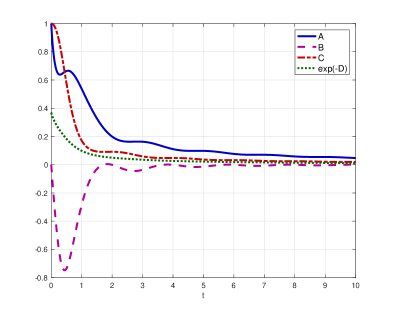
Figure 1: (Colors online.) Evolution of the parameters $A$ (continuous blue line), $B$ (purple dashed line) and $C$ (red dot-dashed line) of the Wigner function (29) in absence of friction ($\eta=0$). The overall normalisation coefficient $\exp(-D)$ (dotted green line) is also shown. We assume to work in arbitrary units in which $m=0.4$, $\tau=1$, $\Lambda_{0}=1$ and $\kappa=1$.

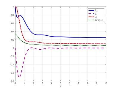
Figure 2: The same as in Figure 1 but with the addition of the friction. The values of the parameters are $m=0.4$, $\tau=1$, $\Lambda_{0}=1$, $\kappa=1$ and $\eta=0.5$.

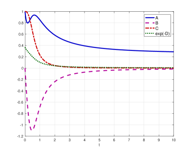
Figure 3: The same as in Figure 2 but with the harmonic potential removed. The values of the parameters are $m=0.4$, $\tau=1$, $\Lambda_{0}=1$, $\kappa=0$ and $\eta=0.5$.

The dissipative character of the new term is clearly seen by computing its moments:

$$\int_{\mathbb{R}}\frac{\partial}{\partial p}\,(pw)\,dp=0,\qquad\frac{1}{m}\int_{\mathbb{R}}p\frac{\partial}{\partial p}\,(pw)\,dp=-J,\qquad\frac{1}{2m}\int_{\mathbb{R}}p^{2}\frac{\partial}{\partial p}\,(pw)\,dp=-2E.$$

These bring dissipative contributions to the Euler system, which takes the new form

$$\left\{\begin{aligned} &\frac{\partial N}{\partial t}+\frac{\partial J}{\partial x}=0,\\[8.0pt] &\frac{\partial J}{\partial t}+\frac{\partial\mathcal{J}_{J}}{\partial x}+\frac{1}{m}\,V^{\prime}N=\frac{\hbar\Lambda_{1}}{m\tau}\,N-\eta J,\\[8.0pt] &\frac{\partial E}{\partial t}+\frac{\partial\mathcal{J}_{E}}{\partial x}+V^{\prime}J=\frac{\hbar\Lambda_{1}}{m\tau}\,J-\frac{\hbar^{2}\Lambda_{2}}{m\tau}\,N-2\eta E.\end{aligned}\right.$$ (35)

6 Conclusions

In this paper we have seen how Wigner equation can be endowed with terms describing a dynamical decoherence mechanism. This is not a novelty, of course, but, as far as we know, this is the first time that the decoherence term has a fairly general form, coming from basic quantum mechanics. In particular, we started from the single-collision decoherence model derived in Ref. [2], which describes the decoherence of a “heavy” particle as a consequence of the collision with a much lighter one. By assuming the heavy particle to undergo multiple random collisions in an environment of light particles, we (formally) derived the Wigner equation (14). The latter admits two contributions from the collisions with the environment: a Hamiltonian part, represented by the function $\Gamma$, and a true decoherence part, represented by the function $\Lambda$, which is nothing but the inverse Fourier transform of the convolution kernel $\gamma$ appearing in the right-hand side of Eq. (14). This picture allows for the interesting interpretation that decoherence smooths out the oscillations of the Wigner function, due to quantum interference, so that the Wigner function tends to a classical distribution in phase-space.

Then, we have seen that when $\Lambda$ assumes particular forms, our model reduces to existing decoherence models. In particular, the largely-used Wigner-Fokker-Planck equation (20) corresponds to the quadratic approximation of $\Lambda$. Moreover, when $1-\Lambda$ is assumed to be a decaying exponential function, our model shows analogies with the Jacoboni-Bordone model [11], in which the exponential decay of the coherence length is embedded ab initio in the definition of the Wigner function. Our analysis, however, allows us to deduce some general features of decoherence (or, at least, of this kind of decoherence), as for example its effects on the dynamics of the macroscopic quantities $N$, $J$ and $E$, i.e. the number, current and energy spatial densities (see Eq. (27)).

A big issue, already addressed in the classical paper by Joos and Zeh [12] is the long time behaviour of decoherence. In Section 5 we have considered the special case of a gaussian Wigner function, for which the Wigner equation (14), in the particular form (28), comes down to an equivalent system if ODEs. In this way we realized that the addition of a Caldeira-Legget quantum friction term [7] produces a physically meaningful behaviour in the long run, since the momentum spread of the particle is stabilised to an asymptotic value. Equivalently, the coherence length, reaches a corresponding asymptotic value.

The addition of the quantum friction fixes the issue of the long-time behaviour, yet it is not completely satisfactory. In fact, as remarked by Arnold et al. [3, 4], the friction + diffusion term (i.e. the right-hand side of Eq. (32)) is not quantum mechanically “correct” (unless $\eta=0$), since it does not satisfy the Lindblad condition, assuring the complete positivity of the evolution [8]. We believe, however, that our analysis indicates the right direction to search for a model that is compatible with the fundamental laws of quantum mechanics and keeps its validity for asymptotically long times.

References

- [1] R. Adami, R. Figari, D. Finco, A. Teta, “On the asymptotic behaviour of a quantum two-body system in the small mass ratio limit”, J. Phys. A: Math. Gen., vol. 37, pp. 7567–7580 (2004)
- [2] R. Adami, M. Hauray, C. Negulescu, . “Decoherence for a heavy particle interacting with a light particle: new analysis and numerics”, Comm. Math.Sci., vol. 14(5), pp. 1373–1415 (2016)
- [3] A. Arnold, J.L. Löpez, P.A. Markowich, J. Soler, “An analysis of quantum Fokker-Planck models: A Wigner function approach”, Rev. Mat. Iberoamericana, vol. 20(3), pp. 771–814 (2004)
- [4] A. Arnold, “Mathematical properties of quantum evolution equations”. In: N. Ben Abdallah, G. Frosali (eds.), Quantum transport. Modelling, analysis and asymptotics, pp. 45–109. Springer, Berlin Heidelberg (2008)
- [5] L. Barletti, “A mathematical introduction to the Wigner formulation of quantum mechanics,” Boll. Unione Mat. Ital. B, vol 6-B(8), pp. 693–716 (2003)
- [6] L. Barletti, G. Frosali, O. Morandi, “Kinetic and hydrodynamic models for multi-band quantum transport in crystals”. In: M. Ehrhardt, T. Koprucki (eds.), Multi-band effective mass approximations: advanced mathematical models and numerical techniques, pp. 3–56. Springer, Berlin Heidelberg (2014)
- [7] A. Caldeira, A. Legget, “Path integral approach to quantum Brownian motion,” Physica, vol. 121A, pp. 587–616 (1983)
- [8] E.B. Davies, Quantum theory of open systems. Academic Press, London (1976)
- [9] P. J. Dodd, J. J. Halliwell, “Decoherence and records for the case of a scattering environment,” Phys. Rev. D, vol. 67, p. 105018 (2003)
- [10] M. Hauray, C. Gomez, “Rigorous derivation of Lindblad equations from quantum jumps processes in 1D”, arXiv:1603.07969 [math-ph] (2016)
- [11] C. Jacoboni, P. Bordone, “Wigner transport equation with finite coherence length”, J. Comput. Electron., vol. 13, pp. 257–267 (2014)
- [12] E. Joos, H.-D. Zeh, “The emergence of classical properties through interaction with the environment”, Z. Phys. B, vol. 59, pp. 223–243 (1985)
- [13] A. Jüngel, Transport Equations for Semiconductors. Springer, Berlin Heidelberg (2009)
- [14] V. Romano, “Quantum corrections to the semiclassical hydrodynamical model of semiconductors based on the maximum entropy principle”, J. Math. Phys., vol. 48, p. 123504 (2007)
- [15] P. Schwaha, D. Querlioz, P. Dollfus, J. Saint-Martin, M. Nedjalkov, S. Selberherr, “Decoherence effects in the Wigner function formalism”, J. Comput. Electron., vol. 12, pp. 388–396 (2013)
- [16] V. I. Tatarskiĭ, “The Wigner representation of quantum mechanics,” Sov. Phys. Usp., vol. 26, pp. 311-327 (1983)
- [17] E. Wigner, “On the quantum correction for thermodynamic equilibrium”, Phys. Rev., vol. 40, pp. 749–759 (1932)
- [18] E. Wigner, “Review of the quantum mechanical measurement problem”. In: P. Meystre, M. Scully (eds.), Quantum optics, experimental gravity and measurement theory, pp. 43–63. Plenum Press, New York (1983)
- [19] C.K. Zachos, D.B. Fairlie, T.L. Curtright (eds.), Quantum mechanics in phase space. An overview with selected papers. World Scientific, Hackensack (2005)
- [20] W. H. Zurek, “Decoherence, einselection, and the quantum origins of the classical”, Rev. Mod. Phys., vol. 75, pp. 715–775 (2003)
- [21] I. Žutić, J. Fabian, S. Das Sarma, “Spintronics: fundamentals and applications”, Rev. Mod. Phys, vol. 76(2), pp. 323–410 (2002)