Cascaded Text Generation
with Markov Transformers

Abstract

The two dominant approaches to neural text generation are fully autoregressive models, using serial beam search decoding, and non-autoregressive models, using parallel decoding with no output dependencies. This work proposes an autoregressive model with sub-linear parallel time generation. Noting that conditional random fields with bounded context can be decoded in parallel, we propose an efficient cascaded decoding approach for generating high-quality output. To parameterize this cascade, we introduce a Markov transformer, a variant of the popular fully autoregressive model that allows us to simultaneously decode with specific autoregressive context cutoffs. This approach requires only a small modification from standard autoregressive training, while showing competitive accuracy/speed tradeoff compared to existing methods on five machine translation datasets.

1 Introduction

Probabilistic text generation is a ubiquitous tool in natural language processing. Originally primarily studied with respect to machine translation [1, 27], its progress has led to applications in document summarization [40, 45], data-to-text [60], image captioning [61], etc. State-of-the-art text generation approaches rely on fully autoregressive models such as RNNs and transformers [53], in which the probability of an output word depends on all previous words. At inference time, beam search is used for decoding, a left-to-right serial procedure. To speed up decoding, researchers have proposed alternative parallel generation models. One class of non-autoregressive probabilistic models assumes that each word’s output probability is independent of other words [13, 67, 28]. While it is impressive that these models perform well, this independence assumption is very strong and often results in noticeable artifacts such as repetitions [13, 51].

We note that non-autoregressive models, while sufficient, are not necessary for fast probabilistic parallel generation. On parallel hardware, inference in models with bounded Markov dependencies is trivial to parallelize and requires sub-linear time w.r.t. sequence length [43, 39]. In practice, given the right parameterization, we can explore any level of autoregressive dependencies to achieve a speed/accuracy tradeoff.

In this work, we exploit this property by proposing cascaded decoding with a Markov transformer architecture. Our approach centers around a graphical model representation of the output space of text generation. Given this model, we can employ cascaded decoding [7, 8, 58, 41] for parallel text generation, using an iterative procedure that starts from a non-autoregressive model and introduces increasingly higher-order dependencies. We combine this approach with a Markov transformer, an extension to the fully autoregressive transformer architecture. This network uses barriers during training to ensure it learns fixed high-order dependencies. At test time, a single network can be used to parameterize a cascade of different graphical models. The Markov transformer only changes self-attention masks and inputs at training, and is applicable to all transformer variants.

Experiments on five machine translation datasets compare this approach to other beam search and non-autoregressive baselines. Our inference approach is comparably fast to non-autoregressive methods while allowing for local dependencies in a principled, probabilistic way. Results validate the competitive accuracy/speed tradeoff of our approach compared to existing methods. The code for reproducing all results is available at https://github.com/harvardnlp/cascaded-generation.

2 Related Work

There has been extensive interest in non-autoregressive/parallel generation approaches, aiming at producing a sequence in parallel sub-linear time w.r.t. sequence length [13, 54, 26, 67, 55, 14, 11, 12, 49, 15, 28, 16, 51, 57, 30, 42, 66, 64, 50]. Existing approaches can be broadly classified as latent variable based [13, 26, 67, 28, 42], refinement-based [25, 49, 14, 15, 11, 30, 12, 64] or a combination of both [42].

Latent-variable approaches factor out the dependencies among output words, such that we can generate each word independently of each other conditioned on those latent variables. The training of these approaches usually employs variational autoencoders, since the log marginal is intractable [21, 38, 31]. The introduced latent variables enable generation in a single forward pass, achieving $O(1)$ time complexity regardless of sequence length, but many of them suffer from generation artifacts such as repetitions [13]. While not using latent variables, our approach could be extended to incorporate them. A notable difference is that the parallel time complexity of this work is not $O(1)$ but $O(\log L)$ w.r.t. sequence length. In practice though, the only $O(\log L)$ part in our approach takes a negligible fraction of total time [51], and our approach reaches comparable speedup compared to existing approaches with $O(1)$ time complexity.

Another line of research uses refinement-based methods, where the model learns to iteratively refine a partially/fully completed hypothesis. Training usually takes the form of masked language modeling [11, 12] or imitating hand-crafted refinement policies [25, 49, 15]. Refinement-based approaches can sometimes reach better performance after multiple forward passes compared to latent variable based approaches which mostly use a single forward pass [15, 11, 42]. While our method superficially resembles refinement, our approach is probabilistic, model-based, and conceptually simpler. Training is by maximum likelihood, requires no hand-designed rules, and allows for activations to be preserved between iterations. A final benefit of our approach is that multiple lengths can be considered at no extra cost, as opposed to generating candidates under different lengths and reranking [11, 51, 28].

Our approach is motivated by structured prediction cascades (SPC) [58]. SPC is a technique in graphical models for graphical model type tasks, where we can specify the length of the sequence beforehand [58]. To the best of our knowledge, we are the first to adapt it to neural text generation. We also go beyond SPC, which uses multiple models, and show how to adapt a single Markov transformer model to learn the entire cascade. While [51] shares our motivation and combines a 0th order model with a 1st order graphical model, they do not consider higher-order models or cascades, or show how to achieve parallel sublinear time. In addition, we use a single Markov transformer to parameterize all log potentials, instead of using additional parameters for pairwise potentials.

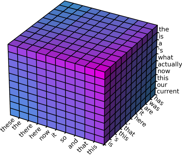
(a) $m=0$

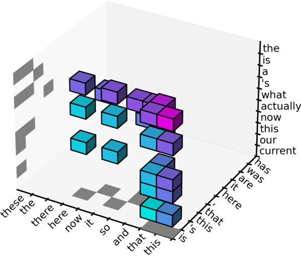
(b) $m=1$

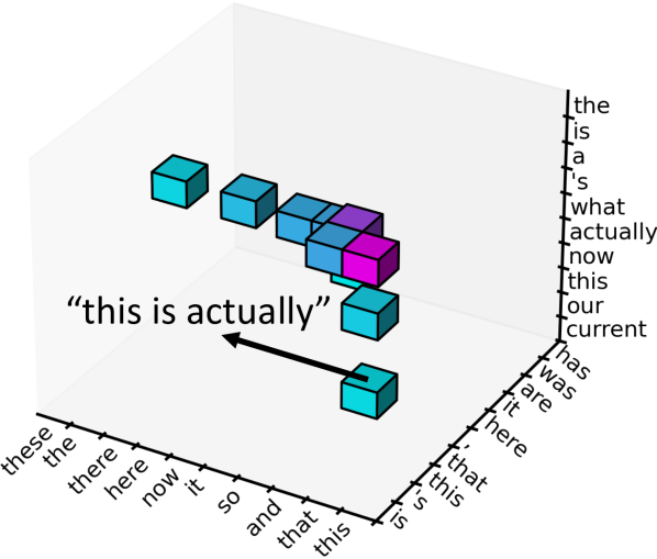
(c) $m=2$

Figure 1: Illustration of cascaded decoding ($K=10$, $\text{iters}=4$) for $\mathcal{X}_{1}$, $\mathcal{X}_{2}$, $\mathcal{X}_{3}$. The axes correspond to $x_{1}$, $x_{2}$ and $x_{3}$. (a) 0th-order (non-autoregressive) model prunes unigrams to produce $\mathcal{X}_{1}$; (b) 1st-order model prunes bigrams to $K$ per size-2 span (seen in 2D projection); (c) 2nd-order model prunes trigrams to $K$ total in size-3 span. Colors represent max-marginals $\text{MM}_{{\cal X}_{m}}^{(m)}(x_{1:3})$, with pink being higher and blue being lower. Fixed limit $K$ allows for efficient parallel (GPU) implementation.

3 Cascaded Decoding for Conditional Random Fields

Neural text decoding can be viewed as a conditional random field (CRF) [24] over a sequence of words $x_{1:L}$, where $x_{i}\in\mathcal{V}$ with $|\mathcal{V}|=V$, and $\mathcal{X}=\mathcal{V}^{L}$ is the set of all sequences. This model defines a conditional probability distribution $P(x_{1:L}|c)$, where $c$ is an arbitrary conditioning term, e.g., a source sentence. Define an $m$-th (Markov) order CRF model as,

$$P^{(m)}(x_{1:L}\ |\ c;\theta)\propto\exp\sum_{l=1}^{L-m}f_{l}^{(m)}(x_{l:{l+m}},c;\theta^{(m)}),$$

where $f^{(m)}_{l}(\cdot)$’s are any parameterized log potentials looking at $m+1$ words, for example local log-probabilities. For simplicity, we omit $c$ and $\theta^{(m)}$ through the rest of this paper. We can define two important special cases of this CRF model. With $m=L-1$, we can recover fully autoregressive neural text generation models such as RNNs and transformers. Using $m=0$ gives us non-autoregressive models.

Decoding aims to find the sequence with the highest model score, $\max_{x^{\prime}\in{\cal X}}P^{(m)}(x^{\prime})$. Computing this exactly can be done with the Viterbi algorithm in $O(V^{m+1}L)$; however, even for $m=1$ this is intractable since $V$ is typically on the order of $10^{4}$. Beam search is commonly used instead to approximate this value, but it cannot be parallelized, and alternatives to beam search remain under-explored in the literature.

We propose an alternative cascaded decoding approach based on max-marginals [58], which are used as a metric to prune “unlikely” n-grams at each position based on the score of the “best” sequence with a given n-gram. To be precise, define the notation ${\cal X}(x_{i:j})$ to be the set of sequences that contain a span $x_{i:j}$, i.e. $\{x^{\prime}\in{\cal X}:x^{\prime}_{i:j}=x_{i:j}\}$. The max-marginal of $x_{i:j}$ is the maximum score in this set:

$$\text{MM}_{\cal X}^{(m)}(x_{i:{j}})=\begin{cases}\displaystyle\max_{x^{\prime}\in{\cal X}(x_{i:j})}P^{(m)}(x^{\prime}_{1:L})&{\cal X}(x_{i:j})\neq\emptyset\\ 0&\text{ o.w. }\end{cases}.$$

Cascaded decoding, illustrated in Figure 1, proceeds by iteratively computing max-marginals for progressively higher-order models while filtering out unlikely spans. Starting with a complete initial set $\mathcal{X}_{0}=\mathcal{X}$, for all single word spans $x_{l:l}$, we compute $M^{(0)}_{\mathcal{X}_{0}}$ and collect the top $K$ max-marginal values at each step to prune the search space,

$$\mathcal{X}_{1}=\{x_{1:L}\in{\cal X}_{0}:x_{l:l}\in\operatorname*{K\,arg\,max}_{x^{\prime}_{l:l}\in{\cal V}^{1}}\text{MM}_{{\cal X}_{0}}^{(0)}(x^{\prime}_{l:l})\text{ for all }l\}.$$

We then apply a 1st order model ($m=1$) and collect the top $K$ $x_{l:l+1}$ values with the highest max marginals $M^{(1)}_{{\cal X}_{1}}(x_{l:l+1})$ to further prune the search space,

$$\mathcal{X}_{2}=\{x_{1:L}\in{\cal X}_{1}:x_{l:l+1}\in\operatorname*{K\,arg\,max}_{x^{\prime}_{l:l+1}\in{\cal V}^{2}}\text{MM}_{{\cal X}_{1}}^{(1)}(x^{\prime}_{l:l+1})\text{ for all }l\}.$$

We repeat the above process $M$ times with increasing $m$, and prune the search space to $\mathcal{X}_{M}$. It can be shown that based on properties of max marginals this set is always non-empty [58]. We decode by finding the sequence $x_{1:L}$ with the highest score $P^{(M)}(x_{1:L})$ in $\mathcal{X}_{M}$.

Given: max length $L$, limit $K$, log potentials $f^{(m)}$ for $m$ in $\{0,\ldots,M\}$, parameters $\theta$

function Cascade( )

     for $m=0\to M-1$ do

         Compute potentials $f_{l}^{(m)}(x_{l:l+m};\theta)$ for all ${\cal X}_{m}(x_{l:l+m})\neq\emptyset$ ($K$) $\triangleright$ $O(K^{2})$

         Compute first-order state relabeling $\Phi^{(m)}_{l}$ for all positions $l=1\ldots L-m$ $\triangleright$ $O(K)$

         Compute max-marginals $\text{MM}_{{\cal X}_{m}}^{(m)}$ using TreeMM$\triangleright$ $O(K^{2}\log L)$

         Set ${\cal X}_{m+1}=\left\{x_{1:L}\in{\cal X}_{m}:x_{l:l+1}\in\displaystyle\operatorname*{K\,arg\,max}_{x^{\prime}_{l:l+m}\in{\cal V}^{m+1}}\text{MM}_{{\cal X}_{m}}^{(m)}(x^{\prime}_{l:l+m})\text{ for all }l\right\}$ $\triangleright$ $O(K^{2})$      

     return $\arg\max_{x^{\prime}\in\mathcal{X}_{M}}P^{(M)}(x^{\prime})$. $\triangleright$ $O(K^{2}\log L)$

function TreeMM(First-order scores $C_{\cdot\cdot\cdot}^{0}$ of size $(L-1)\times K\times K$)

     All $C^{i},S^{i},P^{i}$ size $2^{\log(L-1)-i}\times K\times K$, all $j\in\{0\ldots 2^{\log(L-1)-i}-1\}$

     $P^{\log(L-1)},S^{\log(L-1)}\leftarrow 0$

     for $i=0\to\log(L-1)-2$ do $\triangleright$ Chart max-scores computed bottom-up

         $C^{i+1}_{j\cdot\cdot}\leftarrow\max_{k}C^{i}_{2j\cdot k}+C^{i}_{(2j+1)k\cdot}$      

     for $i=\log(L-1)\to 1$ do $\triangleright$ Prefix and suffix MM scores computed top-down

         $P^{i-1}_{2j\cdot\cdot}\leftarrow P^{i}_{j\cdot\cdot}\ ;\ P^{i-1}_{2j+1\cdot\cdot}\leftarrow\max_{k}P^{i}_{j\cdot k}+C_{2jk\cdot}^{i-1}$

         $S^{i-1}_{2j+1\cdot\cdot}\leftarrow S_{j\cdot\cdot}^{i}\ ;\ S^{i-1}_{2j\cdot\cdot}\leftarrow\max_{k}C^{i-1}_{(2j+1)\cdot k}+S^{i}_{jk\cdot}$      

     return $\exp[(\max_{k}P^{0}_{jk\cdot})+C^{0}_{j\cdot\cdot}+(\max_{k}S^{0}_{j\cdot k})]$ $\triangleright$ $O(K^{2}\log L)$

Algorithm 1 Parallel Cascaded Decoding

Implementation

The only non-parallel component of cascaded decoding is calculation of max-marginals for $m\geq 1$. With $m=1$, max-marginals $x_{l:l+1}$ can be exactly computed using a variant of the forward-backward algorithm. This algorithm requires $O(K^{2}L)$ time when performed serially.

We can reduce this complexity on parallel hardware by leveraging the commutative property of $\max$ [43, 39], and computing an inside-outside prefix sum. First we pad the sequence to a power of 2 and construct a balanced binary tree with words as leaves. We then perform $\max$ operations bottom-up and top down. The height of the tree dictates the parallel time of this approach, $O(K^{2}\log L)$. More details can be found in the TreeMM function in Algorithm 1, where $C^{i}_{j,k_{1},k_{2}}$ is the max possible score of spans $x_{j*2^{i}+1:(j+1)*2^{i}+1}$, with the constraint of the left end being word $k_{1}$ and the right end being word $k_{2}$. We compute $C^{i}$ bottom-up, starting from $i=0$ ($C^{0}$ is the log potentials) and merging adjacent spans in $C^{i}$ to get $C^{i+1}$. The prefix score $P^{i}_{j,k_{1},k_{2}}$ stores the max possible score of $x_{1:j*2^{i}+1}$ (also with end constraints), which we compute iteratively top-down using $P^{i+1}$ and $C^{i}$. Similarly, the suffix score $S^{i}_{j,k_{1},k_{2}}$ is the max score of $x_{(j+1)*2^{i}+1:}$ computed top-down. Finally, we combine the prefix scores $P^{0}$, suffix scores $S^{0}$, and log potentials $C^{0}$ to calculate max marginals of any edge.

For higher-order models with $m>1$, we can compute max-marginals for $x_{l:l+m}$ using a reduction to an $m=1$ CRF. By construction, ${\cal X}_{m}$ has exactly $K$ spans $x_{l:l+m}$ such that ${\cal X}(x_{l:l+m})\neq\emptyset$ for all positions $l$. We relabel these spans $x_{l:l+m}$ as $1\ldots K$ for each position, using a mapping $\Phi^{(m)}_{l}$. This mapping implies that there are at max $K^{2}$ transitions between $\Phi^{(m)}_{l}(x_{l:l+m})$ to $\Phi^{(m)}_{l+1}(x_{l+1:l+m+1})$, resembling an $m=1$ model over $\Phi$. Therefore, the total parallel computation cost is $O(K^{2}\log L)$.

The full procedure is given in Algorithm 1. As opposed to $O(V^{M+1}\log L)$ of exact search, the cascaded approximation can be computed in parallel in $O(MK^{2}\log L)$. We note that this yields a sub-linear time yet (partially) autoregressive decoding algorithm.

Handling Length

A common issue in parallel generation is the need to specify the length of the generation beforehand [13, 28]. It is hard to predict the exact length and constraining search with strict length limits the maximum achievable score. We can relax the length constraint by considering multiple lengths simultaneously. We introduce a special padding symbol pad to $\cal V$ at inference time, and add log-potentials to force pad and end-of-sentence tokens eos to transition to pad. Candidate sequences of different lengths are padded to the same length, but trailing pad’s do not affect scores. The CRF parameterization allows us to consider all these lengths simultaneously, where extending the length only introduces log additional time. More details can be found at supplementary materials.

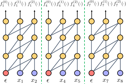
(a)

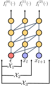
(b)

Figure 2: Markov transformer with $M=2$ and $L=9$. (a) At training, model state is reset with a barrier every $M+1$ words. (b) At decoding, potential $f_{l}^{(0)}$ is computed at each position to get $\mathcal{X}_{1}$, and the dependency order is increased by introducing more columns to compute $\mathcal{X}_{2}$ and $\mathcal{X}_{3}$.

4 Model Parameterization: Markov Transformer

The cascaded decoding approach can be applied to any cascades of CRF models that obey the properties defined above, i.e., $m$-th order log-potentials. Given a training set $(c^{j},x^{j})_{1:J}$ we would like $M+1$ different parameters that satisfy the following MLE objectives:

$$\theta^{(m)}=\arg\max_{\theta^{(m)}}\sum_{j}\log P^{(m)}(x^{j}_{1:L}\ |\ c^{j};\theta^{(m)})\text{ for all }m\in\{0,\ldots M\}$$

Naive approaches for cascading would require training $M+1$ different models that are calibrated or trained together to produce similar outputs [58]. These also cannot be standard translation models such as RNNs or transformers [18, 52, 53], since they have $m=L-1$.

We propose a training and modeling strategy to fix both of these issues. First, to reduce from $M+1$ models to 1, we rewrite the above objective in the form:

$$(\theta^{(0)},\ldots,\theta^{(M)})=\arg\max_{\theta^{(0)}\ldots\theta^{(M)}}\frac{1}{M+1}\sum_{m=0}^{M}\sum_{j}\log P^{(m)}(x^{j}_{1:L}\ |\ c^{j};\theta^{(m)})$$

We then make simplifying assumptions that we only want one set of model parameters $\theta$ and that the Markov order $m$ is sampled through training:

$$\theta=\arg\max_{\theta}\mathbb{E}_{m}\sum_{j}\log P^{(m)}(x^{j}_{1:L}\ |\ c^{j};\theta)$$

In order to approximate this sampling, we train $\theta$ by starting with an autoregressive model and resetting the model’s state every $M+1$ words with a hard barrier. The first barrier is placed uniformly at random from words 1 to $M+1$.

Next, we need a model that can be trained under this hard constraint in order to parameterize $f_{l}^{(m)}(\cdot)$. We propose a variant of the transformer, which we call the Markov transformer (Figure 2), that can satisfy the necessary properties. The model is trained with $(M+1)$-spaced reset barriers with the constraint that self-attention does not cross those barriers. Transformer is particularly suited to learning with this constraint, given that it has positional encodings that encode $l$ even with explicit barriers. In order to ensure that the model can parameterize $P^{(0)}$, i.e., the prediction immediately after the barrier, we replace the first input word by a special token $\epsilon$.

To perform cascaded decoding, we simply start the computation of $f_{l}^{(0)}$ at each position $l$. A benefit of using a single model is that we can reuse the transformer state (neural activations) between iterations, i.e., for $f_{l}^{(m)}(x_{l:l+m})$ we can reuse the cached states from $f_{l}^{(m-1)}(x_{l:l+m-1})$. We use the output of the transformer as the log-potentials. This means each log-potential requires computing one column of the transformer, with length $m$ self-attention, requiring $O(mK)$ parallel time per iteration.

5 Experiments

Datasets

We evaluate our approach on five commonly used machine translation benchmark datasets: IWSLT14 De-En [6] ($\sim$160k parallel sentences), WMT14 En-De/De-En [29] ($\sim$4M parallel sentences) and WMT16 En-Ro/Ro-En [3] ($\sim$610k parallel sentences). To process the data, we use Byte Pair Encoding (BPE) [46, 23] learned on the training set with a shared vocabulary between source and target. For IWSLT14 the vocabulary size is 10k; for WMT14 the vocabulary size 40k. For WMT16 we use the processed data provided by [25]. We sample all validation datasets to be at most 3k.

Model Settings Markov transformer uses the same hyperparameters as standard transformers. The base settings are from FAIRSEQ [34]: For IWSLT14 De-En, we use 6 layers, 4 attention heads, model dimension 512, hidden dimension 1024; for WMT14 En-De/De-En and WMT16 En-Ro/Ro-En we use 6 layers, 8 attention heads, model dimension 512, hidden dimension 2048. We tie the decoder output projection matrix on all datasets [36], and we share source and target embeddings on WMT14 En-De/De-En and WMT16 En-Ro/Ro-En. It differs only in the application of attention barriers, where we set $M=4$. The optimization settings can be found at supplementary materials.

At generation time, we predict the length $L$ using linear regression based on source length. We consider hypotheses of length $L-\Delta L$ to $L+\Delta L$ where we vary $\Delta L$ from 0 to 5. Since the Markov transformer was trained with $M=4$, we consider applying cascaded decoding for 2 to 5 iterations (2 iterations corresponds to $M=1$ in Algorithm 1), where more iterations consider higher local dependency orders at the cost of more computations. The limit $K$ is chosen from $16$, $32$, $64$, $128$.

Baselines For the fully autoregressive baseline, we use the same model setting and use beam size 5. We also compare to other parallel generation methods. These include a latent variable approach: FlowSeq [28]; refinement-based approaches: CMLM [11], Levenshtein transformer [15] and SMART [12]; a mixed approach: Imputer [42]; reinforcement learning: Imitate-NAT [57]; and another sequence-based approach: NART-DCRF [51] which combines a non-autoregressive model with a 1st-order CRF. Several of these methods use fully autoregressive reranking [13], which generally gives further improvements but requires a separate test-time model.

Evaluation We evaluate the BLEU score of different approaches. Following prior works [28, 51, 66], we use tokenized cased BLEU for WMT14 En-De/De-En and tokenized uncased BLEU for IWSLT14 De-En and WMT16 En-Ro/Ro-En, after removing BPE. We measure the average decoding time of a single sentence [13, 25, 16, 15, 55, 51] on a 12GB Nvidia Titan X GPU.

Extension Knowledge distillation [17, 19, 65] is a commonly used technique to improve the performance of parallel generation [13, 25, 28]. In knowledge distillation, we translate the training set using a fully autoregressive transformer and use the translated sentences as the new target for training.

Table 1: Main results. ^†: latency numbers not directly comparable due to platform differences.

Approach		Latency (Speedup) WMT14 En-De		WMT14			WMT16			IWSLT14
Model	Settings			En-De	De-En		En-Ro	Ro-En		De-En
Transformer	(beam 5)	318.85ms	($\times 1.00$)	27.41	31.49		33.89	33.82		34.44
With Distillation
Cascaded Generation	with Speedup
$>\times 7$	(K=16, iters=2)	50.28ms	($\times 6.34$)	26.34	30.69		32.70	32.66		33.90
$>\times 6/5$	(K=32, iters=2)	52.93ms	($\times 6.02$)	26.43	30.72		32.73	32.70		34.01
$>\times 4$	(K=64, iters=2)	68.09ms	($\times 4.68$)	26.52	30.73		32.77	32.76		34.02
$>\times 3$	(K=32, iters=4)	107.14ms	($\times 2.98$)	26.80	31.22		33.14	33.22		34.43
$>\times 2$	(K=32, iters=5)	132.64ms	($\times 2.40$)	26.90	31.15		33.08	33.13		34.43
$>\times 1$	(K=64, iters=5)	189.96ms	($\times 1.68$)	26.92	31.23		33.23	33.28		34.49
Literature
FlowSeq-base [28]			-	21.45	26.16		29.34	30.44		27.55
FlowSeq-large [28]			-	23.72	28.39		29.73	30.72		-
Base CMLM[11]	(iters=10)		-	27.03	30.53		33.08	33.31		-
Levenshtein [15]		92ms	($\times 4.01$)†	27.27	-		-	33.26		-
SMART [12]	(iters=10)		-	27.65	31.27		-	-		-
Imputer [42]	(iters=1)		-	25.8	28.4		-	-		-
imitate-NAT [57]		-	($\times 18.6$)†	22.44	25.67		28.61	28.90		-
NART-DCRF [51]		37ms	($\times 10.4$)†	23.44	27.22		27.44	-		-
Literature+Reranking
FlowSeq-large [28]	(rescoring=30)		-	25.31	30.68		-	-		-
Base CMLM [11]	(iters=4, rescoring 2)	-	($\times 3.0$-$3.1$)†	25.6-25.7	-		-	-		-
imitate-NAT [57]	(rescoring=7)	-	($\times 9.70$)†	24.15	27.28		31.45	31.81		-
NART-DCRF [51]	(rescoring=9)	63ms	($\times 6.14$)†	26.07	29.68		29.99	-		-
NART-DCRF [51]	(rescoring=19)	88ms	($\times 4.39$)†	26.80	30.04		30.36	-		-
Without Distillation
Cascaded Generation	with Speedup
$>\times 7$	(K=16, iters=2)	47.05ms	($\times 6.78$)	21.34	26.91		32.11	32.53		32.95
$>\times 6/5$	(K=32, iters=2)	54.36ms	($\times 5.87$)	22.55	27.56		32.62	32.44		33.14
$>\times 4$	(K=64, iters=2)	69.19ms	($\times 4.61$)	23.09	27.79		32.78	32.43		33.25
$>\times 3$	(K=32, iters=3)	78.29ms	($\times 4.07$)	23.35	28.64		33.12	33.11		33.74
$>\times 2/1$	(K=64, iters=4)	154.45ms	($\times 2.06$)	24.40	29.43		33.64	33.19		34.08
Literature
FlowSeq-base [28]		-		18.55	23.36		29.34	30.44		24.75
FlowSeq-large [28]		-		20.85	25.40		29.73	30.72		-
Levenshtein [15]		126ms	($\times 2.93$)†	25.20	-		-	33.02		-
Literature+Reranking
FlowSeq-large [28]	(rescoring=30)		-	23.64	28.29		32.20	32.84		-

5.1 Results

Results are presented in Table 1. We show the tradeoff between speedup and BLEU score by finding the configuration that gives the best BLEU score with more than $1\times$, $2\times$, $\ldots$, $7\times$ validation speedup. We presented our results in terms of the number of iterations, which is equal to $M+1$, for comparability to refinement-based approaches.

Using knowledge distillation, our results get close to the fully autoregressive baseline: on WMT14 En-De, the gap between our approach and transformer is 0.5 BLEU, while being $2.4\times$ faster ($K=32$, iters=$5$). Our results are also competitive to previous works, even those using a reranker. For example, on WMT14 En-De, we can get $26.52$ BLEU score at a $4.68\times$ speedup, compared to NART-DCRF that reaches $26.80$ BLEU at a $4.39\times$ speedup using 19 candidate sentences to rerank. On IWSLT14, our BLEU scores are much better than previous works: we can reach within 0.54 BLEU score compared to transformer at a $5.88\times$ speedup ($K=16$, iters=2), 6 BLEU points better than FlowSeq.

Our approach is also competitive against previous works without distillation: at a speedup of $2.06\times$, we achieved a better BLEU score than FlowSeq-large using 30 candidates to rerank, which also has many more parameters (66M vs. 258M excluding the reranker). The one model that outperforms our approach is the Levenshtein Transformer. We note though that this model requires hand-crafted rules for training, and uses global communication, while our approach is probabilistic and only requires communicating log potentials between adjacent positions.

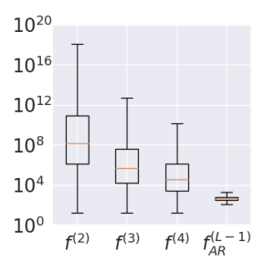
(a)

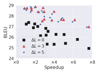
(b)

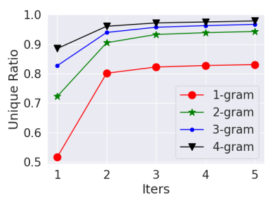
(c)

Figure 3: Analysis on WMT14 En-De val. (a) Box plot of the number of candidate sequences at different dependency orders with $K=16$. Results include cascaded decoding with 3 iterations (scored with $f^{(2)}$), 4 iterations ($f^{(3)}$) and 5 iterations ($f^{(4)}$), and beam baseline ($f^{(L-1)}_{AR}$). (b) BLEU/speedup tradeoff as we vary $\Delta L$. The plot is drawn by varying $K$ from $\{16,32,64,128\}$ and varying iterations from $\{2,3,4,5\}$. (c) The ratio of n-gram repetitions evaluated using the ratio of unique n-grams as a proxy ($K=16$, $\Delta L=0$).

5.2 Analysis

Candidates Searched Unlike beam search, which is limited to a fixed number ($KL$) of candidates, cascaded search can explore an exponential number of sequences [63]. Figure 3 (a) shows the number of candidate sequences scored by cascaded decoding ($f^{(2)}$, $f^{(3)}$, $f^{(4)}$) and beam search ($f_{AR}^{(L-1)}$). We additionally note that max-marginal computations are in practice extremely fast relative to transformer computation and take less than 1% of the total time, so the bottleneck is computing potentials.

Variable Length Generation Cascaded decoding allows for relaxing the length constraint. Figure 3 (b) shows the effect of varying $\Delta L$ from $\{0,3,5\}$, where $\Delta L=0$ corresponds to a hard length constraint, and $\Delta L=3$ sequences of 7 possible length values from $L-3$ to $L+3$. By using $\Delta L=3$, we get more than 1 BLEU improvement at any given speedup. Therefore, we use $\Delta L=3$ for Table 1.

Ratio of Repetitions The independence assumption of non-autoregressive models often leads to visible artifacts in generation such as n-gram repetitions. By introducing higher-order dependencies, we can reduce the ratio of repetitions, as shown in Figure 3 (c), where we measure the extent of repetitions using the ratio of unique n-grams [59]. Cascaded decoding with more than 1 iterations significantly reduces the number of repetitions.

Table 2: Markov transformer with different search strategies on IWSLT14 De-En val w/o distillation. Column $\Delta L$ shows the length constraint ($L-\Delta L$ to $L+\Delta L$), where None denotes no constraint.

Model	Search		Parallel	Time	$\Delta L$	Model Score	BLEU
Transformer [53]	Beam	(K= 5)	N	$O(KL^{2})$	None	-11.82	35.63
Markov Trans.	Beam	(K=5)	N	$O(KML)$	None	-12.05	35.07
	Beam	(K=64)	N	-	$0$	-17.79	33.14
	Beam	(K=1024)	N	-	$0$	-16.77	33.33
	Cascade	(K=64, iters=5)	Y	-	$0$	-17.44	33.45
	Cascade	(K=64, iters=5)	Y	-	$3$	-13.87	35.03

Markov Transformer Analysis Table 2 shows different search algorithms for the Markov transformer. We can observe that 1) a 4th-order Markov transformer is very expressive by itself: using beam search with $K=5$, the BLEU score (35.07) is close to the BLEU score of a transformer (35.63); 2) Cascaded decoding is less effective without distillation than serial beam search; 3) With length constraint, cascaded decoding is more effective than beam search; 4) Variable length generation can improve upon enforcing strict length constraints. Finally, we want to note that Markov transformer’s complexity is lower than normal transformer, since it attends to at most $M$ past words.

Multi-GPU Scaling on multiple GPUs is becoming more important, given the recent trend in bigger models [47, 5]. For multi-GPU parallelization, each GPU takes a chunk of the sequence and forwards decoder for that chunk, while each GPU maintains full encoder states. The only communications between GPUs are the log potentials of size $L\times K\times K$ at each iteration. By using 4 GPUs, our approach can reach speedup of $2.79\times$ compared to $1.68\times$ using only 1 GPU when $K=64$ and $\text{iters}=5$ on WMT14 En-De test set with distillation. Note that we use batch size 1, while for most other approaches due to the global communication required between different parts of the target sentence, it is hard to reach this level of parallelism.

Max-Marginals To prune “unlikely” n-grams at each position, we used max-marginals instead of n-gram scores. The problem with using n-gram scores is that they do not consider compatibility with other positions. Max-marginal fixes this issue with negligible extra time. On WMT14 En-De validation set, using n-gram scores would get a BLEU score of 28.42 at 123.48ms, while using max-marginals reaches 29.24 at 128.58ms ($\text{iters}=5$, $K=32$, $\Delta L=3$).

6 Conclusion

We demonstrate that probabilistic autoregressive models can achieve sub-linear decoding time while retaining high fidelity translations by replacing beam search with a cascaded inference approach. Our approach, based on [58], iteratively prunes the search space using increasingly higher-order models. To support this inference procedure, we utilize Markov transformers, a variant of transformer that can parameterize cascades of CRFs. Experiments on five commonly used machine translation benchmark datasets validate that our approach is competitive in terms of accuracy/speed tradeoff with other state-of-the-art parallel decoding methods, and practically useful with distillation.

Our work opens up a number of exciting future directions, such as applying this approach to longer-form text generation using latent variables, extending the Markov transformer to mimic any specified graphical model, or using more powerful globally normalized energy models instead of locally normalized ones.

Broader Impact

Our work proposes an alternative approach to beam search that enables more efficient text generation. This work primarily uses machine translation as an application, but in the long run, it might be applied to longer-form text generation such as summarizing or translating entire documents, or be deployed to edge devices due to its faster inference and lower computational costs.

On the positive side, more efficient text generation can make these technologies more accessible to the general public. For example, machine translation can help overcome language barriers [37]; document summarization makes data more interpretable [33]. However, there are potential risks. Faster text generation has provoked concerns about generating fake news and targeted propaganda [56, 9] and might pose safety concerns if it was used to generate hate speech or to harass people [48]. Another potential problem is that it might generate language that appears fluent but fabricates facts [22].

To mitigate those issues, there have been works trying to detect machine-generated text [10, 62, 2]. While these works address some concerns over the abuse of text generation, we should be cautious that fake news detection is still a mostly unsolved technical problem and requires active future research [44, 4] as well as non-technical mitigation efforts.

Supplementary Materials for
       Cascaded Text Generation with Markov Transformers

Appendix A: Cascaded Decoding Examples

We show a decoding example in Table 3 ($K=5$, $\Delta L=1$, iters=5). We sort states by max-marginals in descending order and use - to denote invalid states (with $-\infty$ log max-marginals). In this simple sentence, using 1 iteration ($m=0$, non-autoregressive model) repeats the word “woman” ($m=0$, first row, $x_{4:4+m}$). Introducing higher order dependencies fixes this issue.

Table 3: Cascaded Decoding Example. When $m=4$, Viterbi in $\mathcal{X}_{4}$ returns “an amazing woman . eos”. The source is “eine erstaunliche frau . eos” and the target is “an amazing woman . eos”.

$m$	$x_{1:1+m}$	$x_{2:2+m}$	$x_{3:3+m}$	$x_{4:4+m}$	$x_{5:5+m}$	$x_{6:6+m}$	$x_{7:7+m}$	$x_{8}$
0	an	amazing	woman	woman	eos	eos	eos	pad
	amazing	woman	amazing	.	.	pad	pad	-
	incredible	an	an	amazing	woman	.	.	-
	this	remarkable	.	eos	amazing	woman	woman	-
	remarkable	incredible	women	an	women	women	women	-
1	an amazing	amazing woman	woman .	. eos	eos pad	pad pad	pad pad
	an incredible	incredible woman	amazing woman	woman .	. eos	eos pad	eos pad
	this amazing	remarkable woman	women .	amazing woman	woman .	. eos	-
	an remarkable	woman amazing	woman woman	. .	women .	woman eos	-
	amazing woman	amazing women	an amazing	. woman	. .	-	-
2	an amazing woman	amazing woman .	woman .eos	. eos pad	eos pad pad	pad pad pad
	an incredible woman	incredible woman .	women . eos	woman . eos	. eos pad	eos pad pad
	this amazing woman	remarkable woman .	woman woman .	. . eos	woman . eos	. eos pad
	an remarkable woman	amazing women .	woman . .	. woman .	. . eos	-
	an amazing women	amazing woman woman	woman . woman	woman . .	-	-
3	an amazing woman .	amazing woman . eos	woman . eos pad	. eos pad pad	eos pad pad pad
	an incredible woman .	incredible woman . eos	women . eos pad	woman . eos pad	. eos pad pad
	this amazing woman .	remarkable woman . eos	woman woman . eos	. . eos pad	woman . eos pad
	an remarkable woman .	amazing women . eos	woman . . eos	. woman . eos	. . eos pad
	an amazing women .	amazing woman woman .	woman . woman .	woman . . eos	-

Table 4: Cascaded Decoding Example. When $m=4$, Viterbi in $\mathcal{X}_{4}$ returns “what has happened ? eos”. The source is “was ist passiert ? eos” and the target is “what happened ? eos”.

$m$	$x_{1:1+m}$	$x_{2:2+m}$	$x_{3:3+m}$	$x_{4:4+m}$	$x_{5:5+m}$	$x_{6:6+m}$	$x_{7:7+m}$	$x_{8}$
0	what	happened	happened	?	eos	eos	eos	pad
	so	has	?	eos	?	pad	pad	-
	now	did	what	happened	happened	?	?	-
	and	what	happen	happen	happen	happened	.	-
	well	’s	eos	happens	happens	.	happened	-
1	what has	has happened	happened ?	? eos	eos pad	pad pad	pad pad
	so what	what happened	what happened	happened ?	? eos	eos pad	eos pad
	and what	’s happened	happen ?	happens ?	happens ?	? eos	-
	what ’s	did what	what ?	happen ?	happen ?	. eos	-
	now what	did happened	what happens	? ?	happened ?	happened eos	-
2	what has happened	has happened ?	happened ? eos	? eos pad	eos pad pad	pad pad pad
	so what happened	what happened ?	happened ? ?	? ? eos	? eos pad	eos pad pad
	what ’s happened	’s happened ?	happen ? ?	happen ? eos	happened ? eos	happened eos pad
	and what happened	did what ?	happen ? eos	happens ? eos	happen ? eos	. eos pad
	now what happened	did what happened	what happened ?	happened ? eos	happens ? eos	? eos pad
3	what has happened ?	has happened ? eos	happened ? eos pad	? eos pad pad	eos pad pad pad
	so what happened ?	what happened ? eos	happened ? ? eos	? ? eos pad	? eos pad pad
	and what happened ?	’s happened ? eos	what happened ? eos	happened ? eos pad	happens ? eos pad
	what ’s happened ?	has happened ? ?	happen ? eos pad	happens ? eos pad	happen ? eos pad
	now what happened ?	what happened ? ?	happen ? ? eos	happen ? eos pad	happened ? eos pad

In Tables 4, 5, 6, 7, 8 we show more examples from IWSLT14 De-En val.

Table 5: Cascaded Decoding Example. When $m=4$, Viterbi in $\mathcal{X}_{4}$ returns “you ’re happy . eos”. The source is “du bist glücklich . eos” and the target is “you ’re happy . eos”.

$m$	$x_{1:1+m}$	$x_{2:2+m}$	$x_{3:3+m}$	$x_{4:4+m}$	$x_{5:5+m}$	$x_{6:6+m}$	$x_{7:7+m}$	$x_{8}$
0	you	’re	happy	.	eos	eos	eos	pad
	happy	are	lucky	eos	.	pad	pad	-
	your	you	gla@@	happy	happy	.	.	-
	and	’s	good	lucky	?	happy	happy	-
	i	be	fortun@@	ful	you	?	?	-
1	you ’re	’re happy	happy .	. eos	eos pad	pad pad	pad pad
	you are	are happy	lucky .	. .	. eos	eos pad	eos pad
	you be	are lucky	good .	happy .	happy .	. eos	-
	you ’s	be happy	happy happy	ful .	? eos	? eos	-
	and you	’re lucky	happy ful	lucky .	you .	happy eos	-
2	you ’re happy	’re happy .	happy . eos	. eos pad	eos pad pad	pad pad pad
	you are happy	are happy .	lucky . eos	. . eos	. eos pad	eos pad pad
	you be happy	be happy .	happy . .	happy . eos	you . eos	happy eos pad
	you ’re lucky	’re lucky .	happy happy .	ful . eos	? eos pad	? eos pad
	you are lucky	are lucky .	happy ful .	lucky . eos	happy . eos	. eos pad
3	you ’re happy .	’re happy . eos	happy . eos pad	. eos pad pad	eos pad pad pad
	you are happy .	are happy . eos	lucky . eos pad	. . eos pad	. eos pad pad
	you be happy .	be happy . eos	happy . . eos	lucky . eos pad	happy . eos pad
	you ’re lucky .	’re lucky . eos	happy ful . eos	ful . eos pad	? eos pad pad
	you are lucky .	are lucky . eos	happy happy . eos	happy . eos pad	you . eos pad

Table 6: Cascaded Decoding Example. When $m=4$, Viterbi in $\mathcal{X}_{4}$ returns “let ’s move . eos”. The source is “bewe@@ g dich . eos” and the target is “move it . eos”.

$m$	$x_{1:1+m}$	$x_{2:2+m}$	$x_{3:3+m}$	$x_{4:4+m}$	$x_{5:5+m}$	$x_{6:6+m}$	$x_{7:7+m}$	$x_{8}$
0	move	move	.	eos	eos	eos	eos	pad
	let	.	eos	.	.	pad	pad	-
	so	moving	move	?	?	.	.	-
	just	’s	forward	forward	here	?	?	-
	now	let	moving	it	forward	here	here	-
1	let ’s	’s move	move .	. eos	eos pad	pad pad	pad pad
	just move	’s moving	moving .	it .	. eos	eos pad	eos pad
	so move	move forward	move it	forward .	here .	. eos	-
	move .	. forward	move forward	? eos	? eos	? eos	-
	move ’s	. moving	move ?	. .	forward .	-	-
2	let ’s move	’s move .	move . eos	. eos pad	eos pad pad	pad pad pad
	let ’s moving	’s move it	move it .	it . eos	. eos pad	eos pad pad
	move ’s move	’s move forward	move forward .	forward . eos	? eos pad	? eos pad
	move . moving	’s moving .	moving . eos	? eos pad	here . eos	. eos pad
	move ’s moving	’s move ?	move ? eos	. . eos	-	-
3	let ’s move .	’s move . eos	move . eos pad	. eos pad pad	eos pad pad pad
	let ’s move it	’s move it .	move it . eos	it . eos pad	. eos pad pad
	let ’s moving .	’s moving . eos	moving . eos pad	forward . eos pad	here . eos pad
	let ’s move forward	’s move forward .	move forward . eos	? eos pad pad	? eos pad pad
	let ’s move ?	’s move ? eos	move ? eos pad	. . eos pad	-

Table 7: Cascaded Decoding Example. When $m=4$, Viterbi in $\mathcal{X}_{4}$ returns “very , very hard . eos”. The source is “sehr sehr schwer . eos” and the target is “very very hard . eos”.

$m$	$x_{1:1+m}$	$x_{2:2+m}$	$x_{3:3+m}$	$x_{4:4+m}$	$x_{5:5+m}$	$x_{6:6+m}$	$x_{7:7+m}$	$x_{8}$
0	very	difficult	difficult	.	eos	eos	eos	pad
	it	hard	hard	eos	.	pad	pad	-
	really	very	.	difficult	difficult	.	.	-
	extremely	tough	very	hard	hard	difficult	difficult	-
	that	,	tough	very	very	hard	hard	-
1	very ,	, very	very difficult	difficult .	. eos	eos pad	pad pad
	very very	very hard	very hard	hard .	eos pad	pad pad	eos pad
	really ,	very difficult	hard .	. eos	difficult .	. eos	-
	it very	, hard	difficult .	hard eos	hard .	difficult eos	-
	extremely ,	, difficult	tough .	difficult eos	. .	hard eos	-
2	very , very	, very hard	very hard .	hard . eos	. eos pad	eos pad pad
	very very difficult	, very difficult	very difficult .	difficult . eos	eos pad pad	pad pad pad
	very very hard	very difficult .	difficult . eos	. eos pad	. . eos	. eos pad
	really , very	very hard .	hard . eos	hard eos pad	hard . eos	hard eos pad
	it very difficult	, hard .	very hard eos	difficult eos pad	difficult . eos	difficult eos pad
3	very , very hard	, very hard .	very hard . eos	hard . eos pad	. eos pad pad
	very , very difficult	, very difficult .	very difficult . eos	difficult . eos pad	eos pad pad pad
	very very difficult .	very difficult . eos	difficult . eos pad	. eos pad pad	difficult . eos pad
	very very hard .	very hard . eos	hard . eos pad	hard eos pad pad	hard . eos pad
	really , very hard	, very hard eos	very hard eos pad	difficult eos pad pad	. . eos pad

Table 8: Cascaded Decoding Example. When $m=4$, Viterbi in $\mathcal{X}_{4}$ returns “the opposite thing happened . eos”. The source is “das gegenteil passierte . eos” and the target is “the opposite happened . eos”.

$m$	$x_{1:1+m}$	$x_{2:2+m}$	$x_{3:3+m}$	$x_{4:4+m}$	$x_{5:5+m}$	$x_{6:6+m}$	$x_{7:7+m}$	$x_{8}$
0	the	opposite	opposite	happened	eos	eos	eos	pad
	and	contr@@	thing	was	.	pad	pad	-
	so	other	ary	thing	happened	.	.	-
	but	the	happened	did	happening	happened	happened	-
	well	conver@@	was	opposite	happen	happen	happen	-
1	the opposite	opposite thing	thing happened	happened .	. eos	eos pad	pad pad
	the contr@@	contr@@ ary	ary happened	was happening	happening .	. eos	eos pad
	and the	the opposite	opposite happened	thing happened	happened .	pad pad	-
	the other	other thing	thing was	did .	eos pad	. happened eos	-
	so the	opposite opposite	was happened	was happened	. .	-	-
2	the opposite thing	opposite thing happened	thing happened .	happened . eos	. eos pad	eos pad pad
	the contr@@ ary	contr@@ ary happened	ary happened .	was happening .	happening . eos	. eos pad
	and the opposite	the opposite happened	opposite happened .	was happened .	happened . eos	happened eos pad
	the other thing	other thing happened	thing was happening	happened . .	. . eos	pad pad pad
	so the opposite	opposite thing was	thing was happened	thing happened .	-	-
3	the opposite thing happened	opposite thing happened .	thing happened . eos	happened . eos pad	. eos pad pad
	the contr@@ ary happened	contr@@ ary happened .	ary happened . eos	was happening . eos	happening . eos pad
	and the opposite happened	the opposite happened .	opposite happened . eos	was happened . eos	happened . eos pad
	the other thing happened	other thing happened .	thing was happening .	happened . . eos	. . eos pad
	the opposite thing was	opposite thing was happening	thing was happened .	-	-

Appendix B: More Visualizations

(a) $m=0$

(b) $m=1$

(c) $m=2$

Figure 4: Illustration of cascaded decoding ($K=10$, iters=4) for $\mathcal{X}_{1}$, $\mathcal{X}_{2}$, $\mathcal{X}_{3}$.

(a) $m=0$

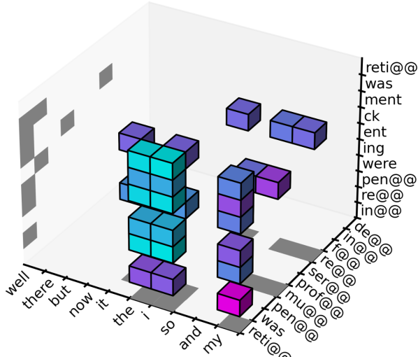
(b) $m=1$

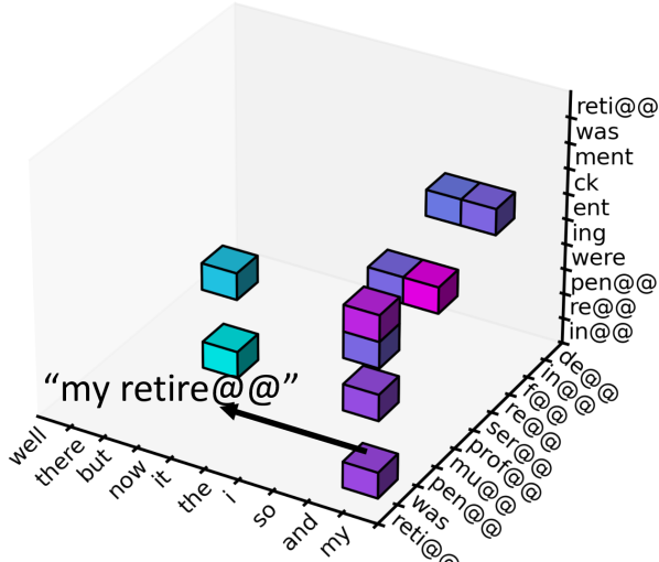
(c) $m=2$

Figure 5: Illustration of cascaded decoding ($K=10$, iters=4) for $\mathcal{X}_{1}$, $\mathcal{X}_{2}$, $\mathcal{X}_{3}$.

We include more visualizations of $\mathcal{X}_{1}$, $\mathcal{X}_{2}$ and $\mathcal{X}_{3}$ in Figure 4 and Figure 5. These examples are taken from IWSLT14 De-En val.

Appendix C: Variable Length Generation Potentials

To handle length, we introduce an additional padding symbol pad to $\mathcal{V}$, and change the log potentials to enforce the considered candidates are of length $L-\Delta L$ to $L+\Delta L$. Note that we can only enforce that for $m\geq 1$, and for $m=0$ we manually add pad to the pruned vocabulary.

We start cascaded search using a sequence of length $L+\Delta L+1$. The main ideas are: 1) We make eos and pad to always transition to pad such that sequences of different lengths can be compared; 2) We disallow eos to appear too early or too late to satisfy the length constraint; 3) We force the last token to be pad such that we don’t end up with sentences without eos endings. Putting these ideas together, the modified log potentials we use are:

$${f^{\prime}}_{l}^{(m)}(x_{l:l+m})$$

$$=\begin{cases}0,\text{ if }x_{l+m-1}=\texttt{eos}\land x_{l+m}=\texttt{pad}\\ -\infty,\text{ if }x_{l+m-1}=\texttt{eos}\land x_{l+m}\neq\texttt{pad}\text{ ($\texttt{eos}$ $\to$ $\texttt{pad}$)}\\ 0,\text{ if }x_{l+m-1}=\texttt{pad}\land x_{l+m}=\texttt{pad}\\ -\infty,\text{ if }x_{l+m-1}=\texttt{pad}\land x_{l+m}\neq\texttt{pad}\text{ ($\texttt{pad}$ $\to$ $\texttt{pad}$)}\\ -\infty,\text{ if }x_{l+m-1}\neq\texttt{pad}\land x_{l+m-1}\neq\texttt{eos}\land x_{l+m}=\texttt{pad}\text{ (nothing else $\to$ $\texttt{pad}$)}\\ -\infty,\text{ if }l+m<L-\Delta L\land x_{l+m}=\texttt{eos}\text{ ($\texttt{eos}$ cannot appear too early)}\\ 0,\text{ if }l+m=L+\Delta L+1\text{ and }x_{l+m}=\texttt{pad}\\ -\infty,\text{ if }l+m=L+\Delta L+1\text{ and }x_{l+m}\neq\texttt{pad}\text{ (the last token must be $\texttt{pad}$)}\\ f_{l}^{(m)}(x_{l:l+m}),\text{ o.t. }\end{cases}.$$

Note that we only considered a single sentence above, but batching is straightforward to implement and we refer interested readers to our code for batch implementations.

Appendix D: Full Results

In the main experiment table we showed latency/speedup results for WMT14 En-De. In Table 9, Table 10, Table 11 and Table 12 we show the latency/speedup results for other datasets. Same as in the main experiment table, we use the validation set to choose the configuration with the best BLEU score under speedup $>\times 1$, $>\times 2$, etc.

Table 9: Results on WMT14 De-En.

Model	Settings	Latency (Speedup)		BLEU
Transformer	(beam 5)	294.64ms	($\times 1.00$)	31.49
With Distillation
Cascaded Generation	with Speedup
$>\times 7$	(K=16, iters=2)	43.41ms	($\times 6.79$)	30.69
$>\times 6$	(K=32, iters=2)	52.06ms	($\times 5.66$)	30.72
$>\times 5$	(K=16, iters=3)	62.06ms	($\times 4.75$)	30.96
$>\times 4/3$	(K=32, iters=3)	79.01ms	($\times 3.73$)	31.08
$>\times 2/1$	(K=32, iters=5)	129.67ms	($\times 2.27$)	31.15
Without Distillation
Cascaded Generation	with Speedup
$>\times 6/5$	(K=32, iters=2)	53.83ms	($\times 5.47$)	27.56
$>\times 4$	(K=32, iters=3)	81.10ms	($\times 3.63$)	28.64
$>\times 3$	(K=32, iters=4)	106.97ms	($\times 2.75$)	28.73
$>\times 2$	(K=64, iters=4)	154.15ms	($\times 1.91$)	29.43
$>\times 1$	(K=128, iters=4)	269.59ms	($\times 1.09$)	29.66

Table 10: Results on WMT16 En-Ro.

Model	Settings	Latency (Speedup)		BLEU
Transformer	(beam 5)	343.28ms	($\times 1.00$)	33.89
With Distillation
Cascaded Generation	with Speedup
$>\times 7$	(K=16, iters=2)	49.38ms	($\times 6.95$)	32.70
$>\times 6$	(K=32, iters=2)	54.56ms	($\times 6.29$)	32.73
$>\times 5$	(K=16, iters=3)	66.33ms	($\times 5.18$)	32.89
$>\times 4$	(K=32, iters=3)	77.39ms	($\times 4.44$)	33.16
$>\times 3$	(K=64, iters=3)	108.57ms	($\times 3.16$)	33.23
$>\times 2$	(K=64, iters=4)	142.23ms	($\times 2.41$)	33.30
$>\times 1$	(K=64, iters=5)	179.07ms	($\times 1.92$)	33.23
Without Distillation
Cascaded Generation	with Speedup
$>\times 7$	(K=16, iters=2)	45.18ms	($\times 7.60$)	32.11
$>\times 6$	(K=32, iters=2)	51.38ms	($\times 6.68$)	32.62
$>\times 5$	(K=16, iters=3)	60.34ms	($\times 5.69$)	32.67
$>\times 4$	(K=32, iters=3)	73.99ms	($\times 4.64$)	33.12
$>\times 3$	(K=64, iters=3)	105.46ms	($\times 3.26$)	33.48
$>\times 2$	(K=64, iters=4)	145.18ms	($\times 2.36$)	33.64
$>\times 1$	(K=128, iters=5)	325.42ms	($\times 1.05$)	33.52

Table 11: Results on WMT16 Ro-En.

Model	Settings	Latency (Speedup)		BLEU
Transformer	(beam 5)	318.57ms	($\times 1.00$)	33.82
With Distillation
Cascaded Generation	with Speedup
$>\times 6/5$	(K=16, iters=2)	46.84ms	($\times 6.80$)	32.66
$>\times 4$	(K=16, iters=3)	62.57ms	($\times 5.09$)	33.00
$>\times 3$	(K=16, iters=5)	99.25ms	($\times 3.21$)	33.04
$>\times 2$	(K=64, iters=3)	103.85ms	($\times 3.07$)	33.17
$>\times 1$	(K=64, iters=5)	181.18ms	($\times 1.76$)	33.28
Without Distillation
Cascaded Generation	with Speedup
$>\times 6$	(K=16, iters=2)	47.58ms	($\times 6.70$)	32.53
$>\times 5$	(K=32, iters=2)	54.05ms	($\times 5.89$)	32.44
$>\times 4$	(K=16, iters=3)	60.94ms	($\times 5.23$)	33.00
$>\times 3$	(K=32, iters=4)	100.29ms	($\times 3.18$)	33.10
$>\times 2$	(K=64, iters=3)	105.21ms	($\times 3.03$)	33.22
$>\times 1$	(K=128, iters=4)	282.76ms	($\times 1.13$)	33.29

Table 12: Results on IWSLT14 De-En.

Model	Settings	Latency (Speedup)		BLEU
Transformer	(beam 5)	229.76ms	($\times 1.00$)	34.44
With Distillation
Cascaded Generation	with Speedup
$>\times 6/5$	(K=16, iters=2)	39.38ms	($\times 5.83$)	33.90
$>\times 4$	(K=32, iters=3)	60.27ms	($\times 3.81$)	34.33
$>\times 3$	(K=32, iters=4)	78.27ms	($\times 2.94$)	34.43
$>\times 2/1$	(K=64, iters=5)	117.90ms	($\times 1.95$)	34.49
Without Distillation
Cascaded Generation	with Speedup
$>\times 5$	(K=64, iters=2)	48.59ms	($\times 4.73$)	33.25
$>\times 4$	(K=32, iters=3)	60.09ms	($\times 3.82$)	33.74
$>\times 3$	(K=64, iters=3)	75.64ms	($\times 3.04$)	33.96
$>\times 2$	(K=64, iters=5)	121.95ms	($\times 1.88$)	34.08
$>\times 1$	(K=128, iters=5)	189.10ms	($\times 1.22$)	34.15

Appendix E: Optimization Settings

Table 13: Optimization settings. We use the same settings for knowledge distillation experiments.

Dataset	dropout	fp16	GPUs	batch	accum	warmup steps	max steps	max lr	weight decay
WMT14 En-De/De-En	0.1	Y	3	4096	3	4k	240k	7e-4	0
WMT16 En-Ro/Ro-En	0.3	Y	3	5461	1	10k	240k	7e-4	1e-2
IWSLT14 De-En	0.3	N	1	4096	1	4k	120k	5e-4	1e-4

Our approach is implemented in PyTorch [35], and we use 16GB Nvidia V100 GPUs for training. We used Adam optimizer [20], with betas 0.9 and 0.98. We use inverse square root learning rate decay after warmup steps [34]. We train with label smoothing strength 0.1 [32]. For model selection, we used BLEU score on validation set. For Markov transformers, we use cascaded decoding with $K=16$ and $\Delta L=3$ to compute validation BLEU score. Other hyperparameters can be found at Table 13.

References

- [1] Dzmitry Bahdanau, Kyunghyun Cho, and Yoshua Bengio. Neural machine translation by jointly learning to align and translate. arXiv preprint arXiv:1409.0473, 2014.
- [2] Anton Bakhtin, Sam Gross, Myle Ott, Yuntian Deng, Marc’Aurelio Ranzato, and Arthur Szlam. Real or fake? learning to discriminate machine from human generated text. arXiv preprint arXiv:1906.03351, 2019.
- [3] Ondřej Bojar, Yvette Graham, Amir Kamran, and Miloš Stanojević. Results of the wmt16 metrics shared task. In Proceedings of the First Conference on Machine Translation: Volume 2, Shared Task Papers, pages 199–231, 2016.
- [4] Alessandro Bondielli and Francesco Marcelloni. A survey on fake news and rumour detection techniques. Information Sciences, 497:38–55, 2019.
- [5] Tom B. Brown, Benjamin Mann, Nick Ryder, Melanie Subbiah, Jared Kaplan, Prafulla Dhariwal, Arvind Neelakantan, Pranav Shyam, Girish Sastry, Amanda Askell, Sandhini Agarwal, Ariel Herbert-Voss, Gretchen Krueger, Tom Henighan, Rewon Child, Aditya Ramesh, Daniel M. Ziegler, Jeffrey Wu, Clemens Winter, Christopher Hesse, Mark Chen, Eric Sigler, Mateusz Litwin, Scott Gray, Benjamin Chess, Jack Clark, Christopher Berner, Sam McCandlish, Alec Radford, Ilya Sutskever, and Dario Amodei. Language models are few-shot learners, 2020.
- [6] Mauro Cettolo, Jan Niehues, Sebastian Stüker, Luisa Bentivogli, and Marcello Federico. Report on the 11th iwslt evaluation campaign, iwslt 2014. In Proceedings of the International Workshop on Spoken Language Translation, Hanoi, Vietnam, volume 57, 2014.
- [7] Eugene Charniak and Mark Johnson. Coarse-to-fine n-best parsing and maxent discriminative reranking. In Proceedings of the 43rd annual meeting on association for computational linguistics, pages 173–180. Association for Computational Linguistics, 2005.
- [8] Eugene Charniak, Mark Johnson, Micha Elsner, Joseph Austerweil, David Ellis, Isaac Haxton, Catherine Hill, R Shrivaths, Jeremy Moore, Michael Pozar, et al. Multilevel coarse-to-fine pcfg parsing. In Proceedings of the main conference on Human Language Technology Conference of the North American Chapter of the Association of Computational Linguistics, pages 168–175. Association for Computational Linguistics, 2006.
- [9] Robert Faris, Hal Roberts, Bruce Etling, Nikki Bourassa, Ethan Zuckerman, and Yochai Benkler. Partisanship, propaganda, and disinformation: Online media and the 2016 us presidential election. Berkman Klein Center Research Publication, 6, 2017.
- [10] Sebastian Gehrmann, Hendrik Strobelt, and Alexander M Rush. Gltr: Statistical detection and visualization of generated text. arXiv preprint arXiv:1906.04043, 2019.
- [11] Marjan Ghazvininejad, Omer Levy, Yinhan Liu, and Luke Zettlemoyer. Constant-time machine translation with conditional masked language models. arXiv preprint arXiv:1904.09324, 2019.
- [12] Marjan Ghazvininejad, Omer Levy, and Luke Zettlemoyer. Semi-autoregressive training improves mask-predict decoding. arXiv preprint arXiv:2001.08785, 2020.
- [13] Jiatao Gu, James Bradbury, Caiming Xiong, Victor OK Li, and Richard Socher. Non-autoregressive neural machine translation. arXiv preprint arXiv:1711.02281, 2017.
- [14] Jiatao Gu, Qi Liu, and Kyunghyun Cho. Insertion-based decoding with automatically inferred generation order. Transactions of the Association for Computational Linguistics, 7:661–676, 2019.
- [15] Jiatao Gu, Changhan Wang, and Junbo Zhao. Levenshtein transformer. In Advances in Neural Information Processing Systems, pages 11179–11189, 2019.
- [16] Junliang Guo, Xu Tan, Di He, Tao Qin, Linli Xu, and Tie-Yan Liu. Non-autoregressive neural machine translation with enhanced decoder input. In Proceedings of the AAAI Conference on Artificial Intelligence, volume 33, pages 3723–3730, 2019.
- [17] Geoffrey Hinton, Oriol Vinyals, and Jeff Dean. Distilling the knowledge in a neural network. arXiv preprint arXiv:1503.02531, 2015.
- [18] Sepp Hochreiter and Jürgen Schmidhuber. Long short-term memory. Neural computation, 9(8):1735–1780, 1997.
- [19] Yoon Kim and Alexander M Rush. Sequence-level knowledge distillation. arXiv preprint arXiv:1606.07947, 2016.
- [20] Diederik P Kingma and Jimmy Ba. Adam: A method for stochastic optimization. arXiv preprint arXiv:1412.6980, 2014.
- [21] Diederik P. Kingma and Max Welling. Auto-Encoding Variational Bayes. In Proceedings of ICLR, 2014.
- [22] Wojciech Kryściński, Bryan McCann, Caiming Xiong, and Richard Socher. Evaluating the factual consistency of abstractive text summarization. arXiv, pages arXiv–1910, 2019.
- [23] Taku Kudo and John Richardson. Sentencepiece: A simple and language independent subword tokenizer and detokenizer for neural text processing. arXiv preprint arXiv:1808.06226, 2018.
- [24] John Lafferty, Andrew McCallum, and Fernando CN Pereira. Conditional random fields: Probabilistic models for segmenting and labeling sequence data. 2001.
- [25] Jason Lee, Elman Mansimov, and Kyunghyun Cho. Deterministic non-autoregressive neural sequence modeling by iterative refinement. arXiv preprint arXiv:1802.06901, 2018.
- [26] Jindřich Libovickỳ and Jindřich Helcl. End-to-end non-autoregressive neural machine translation with connectionist temporal classification. arXiv preprint arXiv:1811.04719, 2018.
- [27] Minh-Thang Luong, Hieu Pham, and Christopher D Manning. Effective approaches to attention-based neural machine translation. arXiv preprint arXiv:1508.04025, 2015.
- [28] Xuezhe Ma, Chunting Zhou, Xian Li, Graham Neubig, and Eduard Hovy. Flowseq: Non-autoregressive conditional sequence generation with generative flow. arXiv preprint arXiv:1909.02480, 2019.
- [29] Matouš Macháček and Ondřej Bojar. Results of the wmt14 metrics shared task. In Proceedings of the Ninth Workshop on Statistical Machine Translation, pages 293–301, 2014.
- [30] Elman Mansimov, Alex Wang, and Kyunghyun Cho. A generalized framework of sequence generation with application to undirected sequence models. arXiv preprint arXiv:1905.12790, 2019.
- [31] Andriy Mnih and Karol Gregor. Neural Variational Inference and Learning in Belief Networks. In Proceedings of ICML, 2014.
- [32] Rafael Müller, Simon Kornblith, and Geoffrey E Hinton. When does label smoothing help? In Advances in Neural Information Processing Systems, pages 4696–4705, 2019.
- [33] Ephraim Nissan. Digital technologies and artificial intelligence’s present and foreseeable impact on lawyering, judging, policing and law enforcement. Ai & Society, 32(3):441–464, 2017.
- [34] Myle Ott, Sergey Edunov, Alexei Baevski, Angela Fan, Sam Gross, Nathan Ng, David Grangier, and Michael Auli. fairseq: A fast, extensible toolkit for sequence modeling. arXiv preprint arXiv:1904.01038, 2019.
- [35] Adam Paszke, Sam Gross, Francisco Massa, Adam Lerer, James Bradbury, Gregory Chanan, Trevor Killeen, Zeming Lin, Natalia Gimelshein, Luca Antiga, et al. Pytorch: An imperative style, high-performance deep learning library. In Advances in Neural Information Processing Systems, pages 8024–8035, 2019.
- [36] Ofir Press and Lior Wolf. Using the output embedding to improve language models. arXiv preprint arXiv:1608.05859, 2016.
- [37] Georg Rehm. Cracking the language barrier for a multilingual europe.
- [38] Danilo Jimenez Rezende, Shakir Mohamed, and Daan Wierstra. Stochastic Backpropagation and Approximate Inference in Deep Generative Models. In Proceedings of ICML, 2014.
- [39] Alexander M Rush. Torch-struct: Deep structured prediction library. arXiv preprint arXiv:2002.00876, 2020.
- [40] Alexander M Rush, Sumit Chopra, and Jason Weston. A neural attention model for abstractive sentence summarization. arXiv preprint arXiv:1509.00685, 2015.
- [41] Alexander M Rush and Slav Petrov. Vine pruning for efficient multi-pass dependency parsing. In Proceedings of the 2012 Conference of the North American Chapter of the Association for Computational Linguistics: Human Language Technologies, pages 498–507. Association for Computational Linguistics, 2012.
- [42] Chitwan Saharia, William Chan, Saurabh Saxena, and Mohammad Norouzi. Non-autoregressive machine translation with latent alignments. arXiv preprint arXiv:2004.07437, 2020.
- [43] Simo Särkkä and Ángel F García-Fernández. Temporal parallelization of bayesian filters and smoothers. arXiv preprint arXiv:1905.13002, 2019.
- [44] Tal Schuster, Roei Schuster, Darsh J Shah, and Regina Barzilay. Are we safe yet? the limitations of distributional features for fake news detection. arXiv preprint arXiv:1908.09805, 2019.
- [45] Abigail See, Peter J Liu, and Christopher D Manning. Get to the point: Summarization with pointer-generator networks. arXiv preprint arXiv:1704.04368, 2017.
- [46] Rico Sennrich, Barry Haddow, and Alexandra Birch. Neural machine translation of rare words with subword units. arXiv preprint arXiv:1508.07909, 2015.
- [47] Mohammad Shoeybi, Mostofa Patwary, Raul Puri, Patrick LeGresley, Jared Casper, and Bryan Catanzaro. Megatron-lm: Training multi-billion parameter language models using gpu model parallelism. arXiv preprint arXiv:1909.08053, 2019.
- [48] Irene Solaiman, Miles Brundage, Jack Clark, Amanda Askell, Ariel Herbert-Voss, Jeff Wu, Alec Radford, and Jasmine Wang. Release strategies and the social impacts of language models. arXiv preprint arXiv:1908.09203, 2019.
- [49] Mitchell Stern, William Chan, Jamie Kiros, and Jakob Uszkoreit. Insertion transformer: Flexible sequence generation via insertion operations. arXiv preprint arXiv:1902.03249, 2019.
- [50] Mitchell Stern, Noam Shazeer, and Jakob Uszkoreit. Blockwise parallel decoding for deep autoregressive models. In Advances in Neural Information Processing Systems, pages 10086–10095, 2018.
- [51] Zhiqing Sun, Zhuohan Li, Haoqing Wang, Di He, Zi Lin, and Zhihong Deng. Fast structured decoding for sequence models. In Advances in Neural Information Processing Systems, pages 3011–3020, 2019.
- [52] Martin Sundermeyer, Ralf Schlüter, and Hermann Ney. Lstm neural networks for language modeling. In Thirteenth annual conference of the international speech communication association, 2012.
- [53] Ashish Vaswani, Noam Shazeer, Niki Parmar, Jakob Uszkoreit, Llion Jones, Aidan N Gomez, Łukasz Kaiser, and Illia Polosukhin. Attention is all you need. In Advances in neural information processing systems, pages 5998–6008, 2017.
- [54] Chunqi Wang, Ji Zhang, and Haiqing Chen. Semi-autoregressive neural machine translation. arXiv preprint arXiv:1808.08583, 2018.
- [55] Yiren Wang, Fei Tian, Di He, Tao Qin, ChengXiang Zhai, and Tie-Yan Liu. Non-autoregressive machine translation with auxiliary regularization. In Proceedings of the AAAI Conference on Artificial Intelligence, volume 33, pages 5377–5384, 2019.
- [56] Claire Wardle and Hossein Derakhshan. Information disorder: Toward an interdisciplinary framework for research and policy making. Council of Europe report, 27, 2017.
- [57] Bingzhen Wei, Mingxuan Wang, Hao Zhou, Junyang Lin, and Xu Sun. Imitation learning for non-autoregressive neural machine translation. arXiv preprint arXiv:1906.02041, 2019.
- [58] David Weiss and Benjamin Taskar. Structured prediction cascades. In Proceedings of the Thirteenth International Conference on Artificial Intelligence and Statistics, pages 916–923, 2010.
- [59] Sean Welleck, Ilia Kulikov, Stephen Roller, Emily Dinan, Kyunghyun Cho, and Jason Weston. Neural text generation with unlikelihood training. arXiv preprint arXiv:1908.04319, 2019.
- [60] Sam Wiseman, Stuart M Shieber, and Alexander M Rush. Challenges in data-to-document generation. arXiv preprint arXiv:1707.08052, 2017.
- [61] Kelvin Xu, Jimmy Ba, Ryan Kiros, Kyunghyun Cho, Aaron Courville, Ruslan Salakhudinov, Rich Zemel, and Yoshua Bengio. Show, attend and tell: Neural image caption generation with visual attention. In International conference on machine learning, pages 2048–2057, 2015.
- [62] Rowan Zellers, Ari Holtzman, Hannah Rashkin, Yonatan Bisk, Ali Farhadi, Franziska Roesner, and Yejin Choi. Defending against neural fake news. In Advances in Neural Information Processing Systems, pages 9051–9062, 2019.
- [63] Wen Zhang, Liang Huang, Yang Feng, Lei Shen, and Qun Liu. Speeding up neural machine translation decoding by cube pruning. arXiv preprint arXiv:1809.02992, 2018.
- [64] Yizhe Zhang, Guoyin Wang, Chunyuan Li, Zhe Gan, Chris Brockett, and Bill Dolan. Pointer: Constrained text generation via insertion-based generative pre-training. arXiv preprint arXiv:2005.00558, 2020.
- [65] Chunting Zhou, Graham Neubig, and Jiatao Gu. Understanding knowledge distillation in non-autoregressive machine translation. arXiv preprint arXiv:1911.02727, 2019.
- [66] Jiawei Zhou and Phillip Keung. Improving non-autoregressive neural machine translation with monolingual data. arXiv preprint arXiv:2005.00932, 2020.
- [67] Zachary M Ziegler and Alexander M Rush. Latent normalizing flows for discrete sequences. arXiv preprint arXiv:1901.10548, 2019.