Uncertainty-Aware Resource Provisioning
for Network Slicing

Abstract

Network slicing allows Mobile Network Operators to split the physical infrastructure into isolated virtual networks (slices), managed by Service Providers to accommodate customized services. The Service Function Chains (SFCs) belonging to a slice are usually deployed on a best-effort premise: nothing guarantees that network infrastructure resources will be sufficient to support a varying number of users, each with uncertain requirements.

Taking the perspective of a network Infrastructure Provider (InP), this paper proposes a resource provisioning approach for slices, robust to a partly unknown number of users with random usage of the slice resources. The provisioning scheme aims to maximize the total earnings of the InP, while providing a probabilistic guarantee that the amount of provisioned network resources will meet the slice requirements. Moreover, the proposed provisioning approach is performed so as to limit its impact on low-priority background services, which may co-exist with slices in the infrastructure network.

A Mixed Integer Linear Programming formulation of the slice resource provisioning problem is proposed. Optimal joint and suboptimal sequential solutions are proposed. These solutions are compared to a provisioning scheme that does not account for best-effort services sharing the common infrastructure network.

I Introduction

Network slicing will play an essential role in 5G communication systems [1, 2, 3]. Leveraging Network Function Virtualization (NFV), network slicing reduces overall equipment and management costs [4] by increasing flexibility in the way the network is operated [5]. Multiple dedicated end-to-end virtual networks or slices can be managed in parallel over a given infrastructure network. With network slicing, vertical markets can be addressed: Customers can manage their own applications by exploiting built-in network slices tailored to their needs [6].

In the extended survey [3] of the so far research efforts in 5G network slicing, the authors provide a taxonomy of network slicing, architectures and future challenges. One of the significant questions is how to meet the slice requirements of different verticals, where multiple network segments including the radio access, transport, and core networks, have to be considered. Infrastructure networks on which slices are operated must support high-quality services with increasing resource consumption (video streaming, telepresence, augmented reality, remote vehicle operation, gaming, etc.). Moreover, the number of users of each slice, their location (usually difficult to predict [7]), and resource demands may fluctuate with time. These uncertainties may impact significantly the resources consumed by each slice and raise the challenging problem of slice resource provisioning. Enough infrastructure resources should be dedicated to a given slice to ensure an appropriate Quality of Service (QoS) despite the uncertainties in the number of slice users and their demands. Over-provisioning should also be avoided, to limit the infrastructure leasing costs and leave resources to concurrent slices.

Existing work on network slicing, see, e.g., [8, 9, 10, 3], is mainly focused on the resource allocation aspect, i.e., assigning infrastructure network resources to virtual network components, with the aim to maximize resource utilization and minimize operation costs. The traffic dynamics in individual slices, such as flow arrival/departure, as well as the dynamics of resource availability on the network infrastructure, may lead to slice QoS below the level expected by the Service Provider (SP) managing the slice. Consequently, to fully unleash the power of network slicing in dynamic environments, uncertainties related to the resource demands need to be carefully addressed.

This paper investigates a method to provision infrastructure resources for network slices, while being robust to a partly unknown number of users with a random usage of the slice resources. Moreover, since some parts of the infrastructure network on which slices should be deployed are often already employed by low-priority background services, the provisioning approach will be performed so as to limit its impact on these services.

The rest of the paper is structured as follows. Section II analyzes related work, and highlights our main contributions. The model of the infrastructure network and of the slice resource demands are presented in Section III. The robust slice resource provisioning problem with uncertainties in the number of users as well as in the resource demands and accounting for the best-effort background services is then formulated in Section IV. The robust slice provisioning problem is transformed into a mixed integer linear programming (MILP) problem in Section V. Numerical results are presented in Section VI. Finally, Section VII draws some conclusions and perspectives.

II Related work

Several works on uncertainty-aware resource allocation for virtual networks can be found in the literature.

In many conventional approaches enough network resources are allocated to make a service available to all users, all the time. In [11], flexible service availability levels are defined, leading to cost savings for the infrastructure provider that can offer overbooked resources for users accepting a service with possibly degraded availability. In the context of network slicing, SPs can benefit from such an approach by providing services with reduced availability or degraded quality to some users ready to accept these conditions. Nevertheless, to evaluate the incidence on the QoS of such under-provisioning mechanism, it is necessary to introduce models of the number of users of a service and of the resource consumption, not considered in [11].

A worst-case allocation at peak traffic is considered in [8, 9]. Nevertheless, this infrastructure resource overbooking is costly and most of the time unnecessary, as all individual slice resource demands are very unlikely peaking simultaneously. In [12], the virtual network embedding problem is solved considering uncertain traffic demands. An MILP formulation is considered, where some of the constraints are required to be satisfied with high probability. In [13], the total deployment costs for cloud computing applications are minimized, while satisfying some QoS constraints. To cope with the uncertain nature of the demands, a stochastic optimization approach is adopted by modeling user demands as random variables obeying normal distributions. Deployment is performed based on the mean demands increased by an integer amount of their standard deviations. This might lead to a conservative solution, requiring more allocated resources than needed. This also reduces somehow the possibility of having service-dependent required confidence levels.

A network slice embedding problem is considered in [14], where available resources and resource demands are assumed to be partly uncertain. They are described by normal distributions built upon the data history on mobile network resource availability as well as slice resource utilization. To control the probability that a slice embedding solution will benefit from enough infrastructure resource, despite the uncertainties, some adjustable safety factor $\gamma$ is introduced. As in [13], enough resources are dedicated to a service so as to satisfy the mean plus $\gamma$ times the standard deviation of the demands. In [14], additionally, a similar approach is considered to account for the uncertainty in the available resources. A probability of feasibility, depending on $\gamma$, is then evaluated for the slice embedding to measure the risk of having a degraded service for some users. The proposed solution leads to a slice resource allocation solution robust to uncertainties. Nevertheless, the resource demands of the different components of the slice have been considered as independent. Moreover, the safety factor $\gamma$ is chosen identical for resource demands and available resources. This again may lead to allocating more resources than strictly necessary, and increases the operation cost.

The network slice embedding problem with demand uncertainties is also addressed in [15]. The minimization of deployment costs considering first static resource demands is formulated as an MILP. Two robust network slice design formulations are then proposed, in uncorrelated and correlated demand uncertainties are considered. In both cases, the objective function is unchanged but some constraints become nonlinear due to the addition of inner maximization problems. These problems account for the upper bound of the resource demands, thus making the network slice embedding problem more complex. A linearization technique inspired by [16] is proposed to relax these inner problems. A tuning parameter $\Gamma$ is introduced to control the trade-off between robustness to the demand uncertainties and the deployment costs. Uncertainties related to the background traffics on the infrastructure, which clearly affect the residual infrastructure resources, are not considered.

To reduce the computation effort required to solve the robust network slice embedding problem, [17] proposes to use a genetic algorithm, shown to surpass the performance of state-of-the-art robust MILP solvers used, e.g., in [15]. Uncertainties in infrastructure link bandwidth are also considered in [18], where possible failures of infrastructure nodes or links are taken into account to propose a robust algorithm that minimizes the network resource consumption under uncertain demands, while remapping the network slice in case of infrastructure failures. Since [15], [17], and [18] assume that the distribution of the variable demands and available infrastructure resource are unknown, their optimization are relatively conservative. Furthermore, uncertainties in various types of resources such as computing, memory, or wireless are not addressed.

In all the above works, the effect of the best effort background services combined with a approach robust to uncertainties in the demands and in the infrastructure resources has not yet been considered for the slice provisioning problem. As shown in the sequel these are two important aspects that need to be taken into account for efficiently providing slices with guaranteed Service Level Agreement (SLA). Finally, we emphasize that these approaches are solving the problem of resource allocation rather than provisioning, i.e., reserving infrastructure resource for a further allocation.

In this paper, we adopt the point of view of the Infrastructure network Provider (InP). We propose a provisioning scheme which aims at maximizing the total earnings of the InP, while providing a probabilistic guarantee that the amount of provisioned network resources will meet the slice requirements. In the provisioning approach, various infrastructure network resources are booked for a slice to satisfy its requirements. Slice resource demands are aggregated. Consequently, resources of several infrastructure nodes may have to be gathered and parallel physical links have to be considered to satisfy these aggregated demands. The provisioning approach may be performed prior to the resource allocation at the time of deployment described, e.g., in [19, 20], where virtual nodes and links are mapped on the infrastructure network. Moreover, instead of considering uncertainties in the available network resource, as in [14], here, we consider best-effort background services running in parallel with the network slices on the infrastructure network. The proposed scheme is able to maintain the impact of resource provisioning on those background services at a prescribed level. Previous results on slice resource provisioning have been presented in [21]. Nevertheless, uncertainties in the number of users of a slice and in the way they consume resources, as well as concurrent best-effort services sharing the infrastructure network have not been taken into account.

III Notations and Hypotheses

A typical network slicing system involves several entities. This may include one or many InPs, Mobile Network Operators (MNOs), and SPs, as depicted in Figure 1 [4]. An InP owns and manages the wireless and wired infrastructure such as the cell sites, the fronthaul and backhaul networks, and cloud data centers. An MNO leases resources from InPs to setup and manage the slices. An SP then exploits the slices supplied by an MNO, and provides to its customers the required services that are running within the slices. Service needs are forwarded by an SP to an MNO within an SLA denoted SM-SLA in what follows.

Figure 1: Network slicing entities and their SLA-based relationships

The SM-SLA describes, at a high level of abstraction, characteristics of the service with the desired QoS. These characteristics may be time-varying due, e.g., to user mobility. In this paper, one considers SM-SLAs composed of: i) a probability mass function (pmf) describing the target number of users/devices to be supported by the slice, ii) a description of the characteristics of the service and of the way it is employed by a typical user/device, and iii) a target probability of service satisfaction. In addition, several time intervals may be considered in the SM-SLA, intervals over each of which the service characteristics and constraints are assumed constant, but may vary from one interval to the next one. These time intervals translate, e.g., day and night variations of user demands. They last between tens of minutes to hours. It is of the responsibility of the SP and MNO to properly scale the requirements expressed in the SM-SLA, by considering, for example, similar services deployed in the past.

Taking the InP perspective, our aim, with resource provisioning is to reserve, somewhat in advance, enough infrastructure resources to ensure that the MNO will be able to provide a slice with characteristics as stated in the SM-SLA it has with the SP. The time scale at which provisioning is performed is much larger than that at which slices are deployed and adapted to meet actual time-varying user demands. In what follows, one focuses on a given time interval over which resources will be provisioned so as to be compliant with the variations of user demands within a slice. The duration of this time interval results from a compromise between the need to update the provisioning and the level of conservatism in the amount of provisioned resources required to satisfy fast fluctuating user demands.

Each slice consists of one or multiple Service Function Chains (SFCs) of different types. An SFC consists of an ordered set of interconnected Virtual Network Functions (VNFs) describing the processing applied to data flows related to a given service. The MNO translates the SP high-level demands into SFCs able to fulfill the service requirements. Based on the characteristics of the service and of its usage, the MNO describes the way the slice (SFCs) resources are consumed by a given user/device. To characterize the variability over time and among users of these demands, we assume that the MNO considers a probabilistic description of the consumption of slice resources by a typical user. The MNO then forwards to the InP these characteristics as part of an SLA between them (MI-SLA). Each InP then provisions infrastructure resources needed for the SFCs. Under the MI-SLA, this provisioning has to meet the target probability of service satisfaction. This translates the fact that enough resources of various types have been provisioned to satisfy the resource demands of the users of the service. This probability is evaluated considering the pmf describing the number of users of the service and the probabilistic description of the slice resource consumption by a typical user. When performing the provisioning, each InP has to limit the impact on other best-effort service running on its infrastructure network.

In this paper, one considers an infrastructure owned by a single InP. To perform the provisioning, the InP has to identify the infrastructure nodes which will provide resources for future deployment of VNFs and the links able to transmit data between these nodes, while respecting the structure of SFCs and optimizing a given objective (e.g., minimizing the infrastructure and software fee costs).

Table I summarizes all parameters involved in the description of the infrastructure network and the graph of SFCs for a slice.

TABLE I: Table of Notations

Symbol	Description
$\mathcal{G}$	Infrastructure network graph, $\mathcal{G}=\left(\mathcal{N},\mathcal{E}\right)$
$\mathcal{N}$	Set of infrastructure nodes
$\mathcal{E}$	Set of infrastructure links
$a_{n}\left(i\right)$	Available resource of type $n$ at node $i$
$a_{\text{b}}\left(ij\right)$	Available bandwidth of link $ij$
$c_{n}\left(i\right)$	Per-unit cost of resource of type $n$ for node $i$
$c_{\text{b}}\left(ij\right)$	Per-unit cost for link $ij$
$c_{\text{f}}\left(i\right)$	Fixed cost for using node $i$
$\mathcal{S}$	Set of slices to be deployed
$\mathcal{G}_{s}$	SFC graph, $\mathcal{G}_{s}=\left(\mathcal{N}_{s},\mathcal{E}_{s}\right)$
$\mathcal{N}_{s}$	Set of VNFs $v$
$\mathcal{E}_{s}$	Set of interconnections $vw$ between VNF $v$ and $w$
$r_{s,n}\left(v\right)$	Fixed amount of resources of type $n$ required
	by an instance of VNF $v$ to operate properly
$r_{s,\text{b}}\left(vw\right)$	Fixed amount of bandwidth to sustain traffic
	demand between VNF instances $v$ and $w$
$U_{s,n}\left(v\right)$	Random amount of resources of type $n$
	of virtual node $v$ employed by a user
$U_{s,\text{b}}\left(vw\right)$	Random amount of bandwidth of virtual link $vw$
	employed by a user
$R_{s,n}\left(v\right)$	Random amount of resources of type $n$
	of virtual node $v$ employed by $N_{s}$ users
$R_{s,\text{b}}\left(vw\right)$	Random amount of bandwidth of virtual link $vw$
	employed by $N_{s}$ users
$B_{s,n}\left(i\right)$	Amount of resources of type $n$ on infrastructure
	node $i$ consumed by background services
$B_{s,\text{b}}\left(ij\right)$	Amount of bandwidth on infrastructure
	link $ij$ consumed by background services

III-A Infrastructure Network

Consider an infrastructure network managed by a given InP. This network is represented by a directed graph $\mathcal{G}=\left(\mathcal{N},\mathcal{E}\right)$, where $\mathcal{N}$ is the set of infrastructure nodes and $\mathcal{E}$ is the set of infrastructure links, which correspond to the wired connections between and within nodes (loopback links) of the infrastructure network.

Each infrastructure node $i\in\mathcal{N}$ is characterized by a given amount of available computing, memory, and wireless resources, denoted as $a_{\text{c}}(i)$, $a_{\text{m}}(i)$, and $a_{\text{w}}\left(i\right)$, which may be allocated to new network slices. These amounts correspond to the total available resources reduced by the amount of resources previously provisioned to concurrent slices. An operation cost paid by the InP is attributed to each unit of node resource. The per-unit node resource cost associated to a given node $i$ consists of a fixed part $c_{\text{f}}\left(i\right)$ for node disposal (paid for each slice using node $i$), and variable parts $c_{\text{c}}(i)$, $c_{\text{m}}(i)$, and $c_{\text{w}}(i)$, which depend linearly on the amount of resources provided by that node.

Similarly, each infrastructure link $ij\in\mathcal{E}$ connecting node $i$ to $j$ has an available bandwidth $a_{\text{b}}\left(ij\right)$, and an associated per-unit bandwidth cost $c_{\text{b}}(ij)$. Several distinct VNFs of the same slice may be deployed on a given infrastructure node. When communication between these VNFs is required, an internal (loopback) infrastructure link $ii\in\mathcal{E}$ can be used at each node $i\in\mathcal{N}$, as in [22], in the case of interconnected virtual machines (VMs) deployed on the same host. The associated per-unit bandwidth cost, in that case, is $c_{\textrm{\text{b}}}\left(ii\right)$.

III-B Graphs of Resource Demands

A demand of resources is defined on the basis of an SLA between an SP and the MNO. As in [21], we consider that a slice is devoted to a single type of service supplied by a given type of SFC. Several instances of that SFC may have to be deployed so as to satisfy the user demand. The topology of each SFC of slice $s$ is represented by a graph $\mathcal{G}_{s}=\left(\mathcal{N}_{s},\mathcal{E}_{s}\right)$ representing the VNFs and their interconnections. Each virtual node $v\in\mathcal{N}_{s}$ represents an instance of a VNF, and each virtual link $vw\in\mathcal{E}_{s}$ represents the connection between virtual nodes $v$ and $w$.

The following weighted graphs are build upon $\mathcal{G}_{s}$.

• $\mathcal{G}_{s}^{\text{r}}=\left(\mathcal{N}_{s}^{\text{r}},\mathcal{E}_{s}^{\text{r}}\right)$ is the graph of Resource Demands of an SFC (SFC-RD) of slice $s$. Each node $v\in\mathcal{N}_{s}^{\text{r}}$ is characterized by a fixed amount of computing $r_{s,\text{c}}(v)$ and memory $r_{s,\text{m}}(v)$ resources allocated by the infrastructure node on which the VNF instance $v$ is deployed to operate properly. Each link $vw\in\mathcal{E}_{s}^{\text{r}}$ is characterized by a given amount of bandwidth $r_{s,\text{b}}(vw)$ that has to be allocated by the infrastructure network to sustain the traffic demand between VNF instances $v$ and $w$.

• $\mathcal{G}_{s}^{\text{U}}=\left(\mathcal{N}_{s}^{\text{U}},\mathcal{E}_{s}^{\text{U}}\right)$ is the graph of Resource Demands a typical User (U-RD) of slice $s$. Each user of slice $s$ is assumed to consume a random proportion of the resources of an SFC of that slice. In addition, the consumed resources by various users are represented by independently and identically distributed random vectors. For a typical user, let $U_{s,\text{c}}\left(v\right)$, $U_{s,\text{m}}\left(v\right)$, $U_{s.\text{w}}\left(v\right)$, and $U_{s,\text{b}}\left(vw\right)$ be the random amount of employed resources of VNF instance $v\in\mathcal{N}_{s}^{\text{r}}$ and of virtual link $vw\in\mathcal{E}_{s}^{\text{r}}$ of the SFC-RD $\mathcal{G}_{s}^{\text{r}}$.

• $\mathcal{G}_{s}^{\text{R}}=\left(\mathcal{N}_{s}^{\text{R}},\mathcal{E}_{s}^{\text{R}}\right)$ is the graph of Resource Demands of Slice $s$ (S-RD). The weight of each node $v\in\mathcal{N}_{s}^{\text{R}}$ and of each link $vw\in\mathcal{E}_{s}^{\text{R}}$ represents the aggregate amount of resources employed by a random number $N^{s}$ of independent users of slice $s$. These amounts are described by random variables denoted as $R_{s,\text{c}}\left(v\right)$, $R_{s,\text{m}}\left(v\right)$, $R_{s,\text{w}}\left(v\right)$, and $R_{s,\text{b}}\left(vw\right)$, for computing, memory, wireless, and bandwidth demand, respectively.

Considering the analysis of co-allocated online services of large scale data centers reported in [23], the utilization of CPU and memory of virtual machines (VMs) have a positive correlation in the majority of cases. Moreover, this correlation is particularly strong at the VMs that execute the same jobs, showing correlation coefficients larger than $0.85$. Based on this observation, for a typical user, the resource demands of different types for a given node $v\in\mathcal{N}_{s}^{\text{U}}$ are considered to be correlated. The demands for resources of the same type among virtual nodes are also correlated. Finally, the resulting traffic demands between nodes is usually also correlated with the resource demands for a given virtual node. To represent this correlation, consider the vector of joint resource demands for a typical user of an SFC of slice $s$

$$\mathbf{U}_{s}=\left(U_{s,\text{c}}\left(v\right),U_{s,\text{m}}\left(v\right),U_{s,\text{w}}\left(v\right),U_{s,\text{b}}\left(vw\right)\right)_{\left(v,vw\right)\in\mathcal{G}_{s}^{\text{U}}}^{\top}.$$

Assuming that $U_{s,\text{c}}\left(v\right)$, $U_{s,\text{m}}\left(v\right)$, $U_{s.\text{w}}\left(v\right)$, and $U_{s,\text{b}}\left(vw\right)$ are normally distributed, $\mathbf{U}_{s}$ follows a multivariate normal distribution with probability density

$$f\left(\mathbf{x};\boldsymbol{\mu}_{s},\boldsymbol{\Gamma}_{s}\right)=\frac{1}{\sqrt{\left(2\pi\right)^{\textrm{card}\left(\mathbf{U}_{s}\right)}\left|\boldsymbol{\Gamma}_{s}\right|}}e^{-\frac{1}{2}\left(\mathbf{x}-\boldsymbol{\mu}_{s}\right)^{\top}\left(\boldsymbol{\Gamma}_{s}\right)^{-1}\left(\mathbf{x}-\boldsymbol{\mu}_{s}\right)},$$ (1)

with mean

$$\boldsymbol{\mu}_{s}=\left(\mu_{s,\text{c}}\left(v\right),\mu_{s,\text{m}}\left(v\right),\mu_{s,\text{w}}\left(v\right),\mu_{s,\text{b}}\left(vw\right)\right)_{\left(v,vw\right)\in\mathcal{G}_{s}^{\text{U}}}^{\top},$$

and covariance matrix $\boldsymbol{\Gamma}_{s}$ such that

$$\text{diag}\left(\boldsymbol{\Gamma}_{s}\right)=\left(\sigma_{s,\text{c}}^{2}\left(v\right),\sigma_{s,\text{m}}^{2}\left(v\right),\sigma_{s,\text{w}}^{2}\left(v\right),\sigma_{s,\text{b}}^{2}\left(vw\right)\right)_{\left(v,vw\right)\in\mathcal{G}_{s}^{\text{U}}}^{\top},$$

the off-diagonal elements of $\boldsymbol{\Gamma}_{s}$ representing the correlation between different types of resource demands. In (1), $\textrm{card}\left(\mathbf{U}_{s}\right)$ is the number of elements of $\mathbf{U}_{s}$. One has thus $U_{s,n}(v)\sim\mathcal{N}\left(\mu_{s,n}\left(v\right),\sigma_{s,n}^{2}\left(v\right)\right)$, with $n\in\left\{\text{c},\text{m},\text{w}\right\}$ and $U_{s,\text{b}}\left(vw\right)\sim\mathcal{N}\left(\mu_{s,\text{b}}\left(vw\right),\sigma_{s,\text{b}}^{2}\left(vw\right)\right)$.

Assume that the number of users $N_{s}$ to be supported by slice $s$ is described by the pmf

$$p_{k}=\Pr\left(N_{s}=k\right).$$ (2)

Since the amount of resources of VNF $v$ and of virtual link $vw$ consumed by different users is represented by independently and identically distributed copies of $\mathbf{U}_{s}$, the joint distribution of the aggregate amount $\mathbf{U}_{s,k}$ of resources consumed by $k$ independent users is $f\left(\mathbf{x},k\boldsymbol{\mu}_{s},k^{2}\boldsymbol{\Gamma}_{s}\right)$. The total amount of resources employed by a random number $N_{s}$ of independent users, $\mathbf{R}_{s}=\mathbf{U}_{s,N_{s}}=\left(R_{s,\text{c}}\left(v\right),R_{s,\text{m}}\left(v\right),R_{s,\text{w}}\left(v\right),R_{s,\text{b}}\left(vw\right)\right)_{\left(v,vw\right)\in\mathcal{G}_{s}^{\text{R}}}^{\top}$ , is distributed according to

$$g\left(\mathbf{x},\boldsymbol{\mu}_{s},\boldsymbol{\Gamma}_{s}\right)=\sum_{k=0}^{\infty}p_{k}f\left(\mathbf{x},k\boldsymbol{\mu}_{s},k^{2}\boldsymbol{\Gamma}_{s}\right).$$ (3)

The typical joint distribution of two components of $\mathbf{U}_{s}$ and $\mathbf{R}_{s}$ is illustrated in Figure 2. Considering a virtual node $v$ of a given slice $s$, Figure 2 represents the joint distribution $f\left(\mathbf{x};\boldsymbol{\mu}_{s},\boldsymbol{\Gamma}_{s}\right)$ of $U_{s,\text{c}}\left(v\right)$ and $U_{s,\text{m}}\left(v\right)$ and the resulting joint distribution $g\left(\mathbf{x},\boldsymbol{\mu}_{s},\boldsymbol{\Gamma}_{s}\right)$ of $R_{s,\text{c}}\left(v\right)$ and $R_{s,\text{m}}\left(v\right)$. Here $N_{s}$ follows the binomial distribution $N_{s}\sim\mathcal{B}\left(10,0.5\right)$, $\boldsymbol{\mu}_{s}=\left[2,3\right]^{\top}$. In Figure 2a, $\boldsymbol{\Gamma}_{s}=\left[\begin{array}[]{cc}1&0\\ 0&1\end{array}\right]$ is diagonal. Even if the level sets of $f\left(\mathbf{x};\boldsymbol{\mu}_{s},\boldsymbol{\Gamma}_{s}\right)$ are circles, the level sets of the resulting $g\left(\mathbf{x},\boldsymbol{\mu}_{s},\boldsymbol{\Gamma}_{s}\right)$ illustrate the correlation between $R_{s,\text{c}}\left(v\right)$ and $R_{s,\text{m}}\left(v\right)$. In Figure 2b, $\boldsymbol{\Gamma}_{s}=\left[\begin{array}[]{cc}1&0.85\\ 0.85&1\end{array}\right]$ is non-diagonal, i.e., $U_{s,\text{c}}\left(v\right)$ and $U_{s,\text{m}}\left(v\right)$ are correlated, the correlation between $R_{s,\text{c}}\left(v\right)$ and $R_{s,\text{m}}\left(v\right)$ increases significantly.

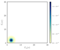
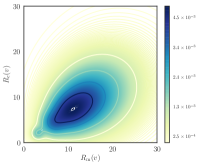
(a) Uncorrelated demands

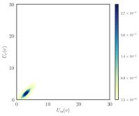
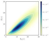
(b) Correlated demands

Figure 2: Joint distribution $f\left(\mathbf{x};\boldsymbol{\mu}_{s},\boldsymbol{\Gamma}_{s}\right)$ (top left and bottom left) and $g\left(\mathbf{x},\boldsymbol{\mu}_{s},\boldsymbol{\Gamma}_{s}\right)$ (top right and bottom right), when $U_{s,\text{c}}\left(v\right)$ and $U_{s,\text{m}}\left(v\right)$ are (a) uncorrelated, and (b) correlated.

III-C Resource Consumption of Best-Effort Background Services

In the considered time interval, a given part of the available resources is consumed by other best-effort background services for which no resource provisioning has been performed. The aggregate amount of resources consumed by these best-effort services is represented by random variables $B_{\text{c}}\left(i\right)$ , $B_{\text{m}}\left(i\right)$ and $B_{\text{w}}\left(i\right)$, $\forall i\in\mathcal{N}$, and $B_{\text{b}}\left(ij\right)$, $\forall ij\in\mathcal{E}$. Each of those variables is assumed to be uncorrelated and Gaussian distributed, $B_{n}\left(i\right)\sim\mathcal{N}\left(\mu_{\text{B},n}\left(i\right),\sigma_{\text{B},n}^{2}\left(i\right)\right)$, $\forall i\in\mathcal{N}$, $\forall n\in\left\{\text{c},\text{m},\text{w}\right\}$, and $B_{n}\left(i\right)\sim\mathcal{N}\left(\mu_{\text{B},\text{b}}\left(ij\right),\sigma_{\text{B},\text{b}}^{2}\left(ij\right)\right)$, $\forall ij\in\mathcal{E}$. Finally, denote $\mathbf{B}=\left(B_{\text{c}}\left(i\right),B_{\text{m}}\left(i\right),B_{\text{b}}\left(ij\right)\right)_{\left(i,ij\right)\in\mathcal{G}}^{\top}$ as the vector gathering all resource consumption of the background services. $\mathbf{B}$ is distributed according to $f\left(\mathbf{x};\boldsymbol{\mu}_{\text{B}},\boldsymbol{\Gamma}_{\text{B}}\right)$, with

$$\boldsymbol{\mu}_{\text{B}}=\left(\mu_{\text{B},\text{c}}\left(i\right),\mu_{\text{B},\text{m}}\left(i\right),\mu_{\text{B},\text{w}}\left(i\right),\mu_{\text{B},\text{b}}\left(ij\right)\right)_{\left(i,ij\right)\in\mathcal{G}}^{\top}$$

and

$$\boldsymbol{\Gamma}_{\text{B}}=\text{diag}\left(\sigma_{\text{B},\text{c}}^{2}\left(i\right),\sigma_{\text{B},\text{m}}^{2}\left(i\right),\sigma_{\text{B},\text{w}}^{2}\left(i\right),\sigma_{\text{B},\text{b}}^{2}\left(vw\right)\right)_{\left(i,ij\right)\in\mathcal{G}}^{\top},$$

since the elements of $\mathbf{B}$ are assumed to be uncorrelated.

IV Optimal Slice Resource Provisioning

Consider a set of slices $\mathcal{S}$ for which infrastructure resources have to be provisioned. To provision resource for a given slice $s\in\mathcal{S}$, the InP has to determine the amount of resources each of its infrastructure nodes and links has to reserve to satisfy the slice resource demands with a given probability. Moreover, the InP has to preserve enough resource for background services. This will be done by evaluating and bounding the probability that the provisioning impacts (reduces) the resources and traffic involved by best effort services.

The slice resource provisioning is represented by a mapping between the infrastructure graph $\mathcal{G}$ and the S-RD graph $\mathcal{G}_{s}^{\text{R}}$, as depicted in Figure 3. In this example, the slice $s$ consists of several linear SFCs of the same type. The mapping has to be performed so as to minimize the provisioning costs, while being able to satisfy the uncertain slice demands with a high probability. The constraints that have to be satisfied by this mapping are detailed in the following sections.

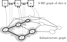
Figure 3: Provisioning of infrastructure resource to slice. In this example, aggregate resources from the infrastructure node pair $\left(i_{1},i_{2}\right)$ is provisioned for the virtual node $v\in\mathcal{N}_{s}^{\text{R}}$ of the S-RD graph of slice $s$. Also, resources gathered from the node pair $\left(j_{1},j_{2}\right)$ is used for $w$. Correspondingly, two infrastructure links $\left(i_{1}j_{1}\right)$ and $\left(i_{2}j_{2}\right)$ (highlighted by the bold and dashed lines) are used to provision resource for the virtual link $vw\in\mathcal{E}_{s}^{\text{R}}$ of the S-RD graph of slice $s$.

Let $\kappa_{s}\left(i,v\right)r_{s,n}(v)$ be the amount of resource of type $n\in\left\{\text{c},\text{m},\text{w}\right\}$ provisioned by node $i$ for a VNF of type $v$, with $\kappa_{s}\left(i,v\right)\in\mathbb{N}_{0}$. Consequently $\kappa_{s}\left(i,v\right)$ represents the number of VNF instances of type $v\in\mathcal{N}_{s}$ that node $i$ will be able to host. Similarly, let $\kappa_{s}\left(ij,vw\right)r_{s,\text{b}}(vw)$ be the bandwidth provisioned by link $ij$ to support the traffic between virtual nodes of type $v$ and $w$.

A solution of the provisioning problem for slice $s$ is thus defined by a given assignment of the variables $\boldsymbol{\kappa}_{s}=\left\{\kappa_{s}\left(i,v\right),\kappa_{s}\left(ij,vw\right)\right\}_{\left(i,ij\right)\in\mathcal{G},\left(v,vw\right)\in\mathcal{G}_{s}^{\text{R}}}$. This assignment has to satisfy some constraints to ensure a satisfying behavior of the SFC and the satisfaction of the MI-SLA for slice $s$ defined in terms of probability of satisfaction of the aggregate user demands $\underline{p}_{s}$, see Section IV-A. In addition, from the perspective of the InP, this assignment has also to have a limited impact on the operation of background best-effort services.

IV-A Constraints

Consider slice $s$ and a given assignment of the variables $\boldsymbol{\kappa}_{s}$. For a given node $v\in\mathcal{N}_{s}^{\text{R}}$, the probability that enough resources are provisioned in the infrastructure network to satisfy the resource demand $R_{s,n}\left(v\right)$ of type $n\in\left\{\text{c},\text{m},\text{w}\right\}$ is

$$p_{s,n}\left(v\right)=\Pr\Big{\{}\sum\limits_{i}\kappa_{s}\left(i,v\right)r_{s,n}\left(v\right)\geqslant R_{s,n}\left(v\right)\Big{\}}.$$ (4)

Similarly, for a given virtual link $vw\in\mathcal{E}_{s}^{\text{R}}$, the probability that enough bandwidth is provisioned in the infrastructure network to satisfy the demand $R_{s,\text{b}}\left(vw\right)$ is

$$p_{s,\text{b}}\left(vw\right)=\Pr\Big{\{}\sum\limits_{ij}\kappa_{s}\left(ij,vw\right)r_{s,\text{b}}\left(vw\right)\geqslant R_{s,\text{b}}\left(vw\right)\Big{\}}.$$ (5)

In both cases, the assignment has to be such that, for each infrastructure node $i\in\mathcal{N}$ and link $ij\in\mathcal{E}$, the total amount of provisioned resources for all slices $s\in\mathcal{S}$ is less or equal than the amount of available resources

$$\sum\limits_{s,v}\kappa_{s}\left(i,v\right)r_{s,n}\left(v\right)\leqslant a_{n}\left(i\right),$$ (6)

$$\sum\limits_{s,vw}\kappa_{s}\left(ij,vw\right)r_{s,\text{b}}\left(vw\right)\leqslant a_{\text{b}}\left(ij\right).$$ (7)

The constraints (6)-(7) may leave no resources for the background best-effort services. The probability that the background best-effort services are impacted at a node $i$ or on the link $ij$ by the provisioning for all slices $s\in\mathcal{S}$ are, $\forall n\in\left\{\text{c},\text{m},\text{w}\right\}$,

$$p_{n}^{\text{im}}\left(i\right)=\Pr\Big{\{}\sum_{s,v}\kappa_{s}\left(i,v\right)r_{s,n}\left(v\right)\geqslant a_{n}\left(i\right)-B_{n}\left(i\right)\Big{\}}$$ (8)

and

$$p_{\text{b}}^{\text{im}}\left(ij\right)=\Pr\Big{\{}\sum_{s,vw}\kappa_{s}\left(ij,vw\right)r_{s,\text{b}}\left(vw\right)\geqslant a_{\text{b}}\left(ij\right)-B_{\text{b}}\left(ij\right)\Big{\}}.$$ (9)

The impact probabilities (IPs) of the provisioning for all slice $s\in\mathcal{S}$ on the nodes and links resources employed by best-effort service has to be such that, $\forall\left(i,ij\right)\in\mathcal{G}$, $\forall n\in\left\{\text{c},\text{m},\text{w}\right\}$

$$p_{n}^{\text{im}}\left(i\right)\leqslant\overline{p}^{\text{im}},$$ (10)

$$p_{\text{b}}^{\text{im}}\left(ij\right)\leqslant\overline{p}^{\text{im}},$$ (11)

where $\overline{p}^{\text{im}}$ is the maximum tolerated impact probability. The value of $\overline{p}^{\text{im}}$ is chosen by the InP to provide sufficient resources for the background services at every infrastructure nodes and links. A small value of $\overline{p}^{\text{im}}$ leads to a small impact of slice resource provisioning on background services, but makes the provisioning problem more difficult to solve compared to a value of $\overline{p}^{\text{im}}$ close to one.

The considered assignment has to satisfy additional constraints to ensure that the data can be correctly carried between VNFs. For each virtual link $vw\in\mathcal{E}_{s}^{\text{R}}$, resources on a sequence of infrastructure links must be provisioned between each pair of infrastructure nodes that have provisioned resources to the virtual nodes $v$ and $w$. One obtains a flow conservation constraint similar to that introduced in [21]. One should have $\forall s\in\mathcal{S}$, $\forall i\in\mathcal{N}$, $\forall vw\in\mathcal{E}_{s}$,

$$\sum\limits_{j\in\mathcal{N}}\left[\kappa_{s}\left(ij,vw\right)-\kappa_{s}\left(ji,vw\right)\right]$$

$$=\left(\frac{r_{s,\text{b}}(vw)}{{\scriptstyle\sum_{vu}}r_{s,\text{b}}(vu)}\right)\kappa_{s}\left(i,v\right)-\left(\frac{r_{s,\text{b}}(vw)}{{\scriptstyle\sum_{uw}}r_{s,\text{b}}(uw)}\right)\kappa_{s}\left(i,w\right).$$ (12)

Finally, considering an assignment $\boldsymbol{\kappa}=\left\{\boldsymbol{\kappa}_{s}\right\}_{s\in\mathcal{S}}$ which satisfies (6)-(12), the probability that this assignment is compliant with the constraints imposed for slice $s$ and by the infrastructure, i.e., the Probability of Successful Provisioning (PSP) for slice $s$ is

$$\begin{array}[]{clcl}p_{s}\left(\boldsymbol{\kappa}_{s}\right)=\Pr\Big{\{}&\sum\limits_{i}\kappa_{s}\left(i,v\right)r_{s,n}\left(v\right)&\geqslant&R_{s,n}\left(v\right),\forall v,n,\\ &\sum\limits_{ij}\kappa_{s}\left(ij,vw\right)r_{s,\text{b}}\left(vw\right)&\geqslant&R_{s,\text{b}}\left(vw\right),\forall vw\Big{\}},\end{array}$$ (13)

and, as stated in the MI-SLA, the InP has to ensure a minimum PSP of $\underline{p}_{s}$ for every slice $s\in\mathcal{S}$, i.e.,

$$p_{s}\left(\boldsymbol{\kappa}_{s}\right)\geqslant\underline{p}_{s}.$$ (14)

IV-B Costs, Incomes, and Earnings

Considering the perspective of the InP, this section presents the cost, income, and earnings model for the slice resource provisioning problem.

Consider a given slice $s\in\mathcal{S}$ and its related assignment of the variables $\boldsymbol{\kappa}_{s}$. Let

$$x_{s}\left(\boldsymbol{\kappa}_{s}\right)=\begin{cases}1&\text{if }p_{s}\left(\boldsymbol{\kappa}_{s}\right)\geqslant\underline{p}_{s}\\ 0&\text{else}\end{cases}$$ (15)

indicate whether the MI-SLA for slice $s$ is satisfied.

Define $I_{s}$ as the income obtained for a slice $s$ whose MI-SLA is satisfied. The income awarded to the InP from the MNO is then $I_{s}x_{s}\left(\boldsymbol{\kappa}_{s}\right)$.

The total provisioning cost $C_{s}$$\left(\boldsymbol{\kappa}_{s}\right)$ of a given slice $s$ for the InP is

$$C_{s}\left(\boldsymbol{\kappa}_{s}\right)= \sum\limits_{i}\widetilde{\kappa}_{s}\left(i\right)c_{\textrm{f}}\left(i\right)+\sum\limits_{i,v,n}\kappa_{s}\left(i,v\right)r_{s,n}\left(v\right)c_{n}\left(i\right)$$

$$+ \sum\limits_{ij,vw}\kappa_{s}\left(ij,vw\right)r_{s,\text{b}}\left(vw\right)c_{\text{b}}\left(ij\right),$$ (16)

where

$$\widetilde{\kappa}_{s}\left(i\right)=\begin{cases}1&\text{if }\sum_{v}\kappa_{s}\left(i,v\right)>0,\\ 0&\text{otherwise.}\end{cases}$$ (17)

The first term of $C_{s}\left(\boldsymbol{\kappa}_{s}\right)$ represents the fixed costs associated to the use of infrastructure nodes by slice $s$, whereas the second and the third terms indicate the cost of reserved resources from infrastructure nodes and links. The variable $\widetilde{\kappa}_{s}\left(i\right)$ indicates whether the infrastructure node $i$ is used by slice $s$.

Finally, the total earnings $E_{s}\left(\boldsymbol{\kappa}_{s}\right)$ obtained by the InP for the successful provisioning of slice $s$ is

$$E_{s}\left(\boldsymbol{\kappa}_{s}\right)=I_{s}x_{s}\left(\boldsymbol{\kappa}_{s}\right)-C_{s}\left(\boldsymbol{\kappa}_{s}\right).$$ (18)

IV-C Nonlinear Constrained Optimization Problem

Consider a set of slices $\mathcal{S}$, the resource provisioning problem for all slices $s\in\mathcal{S}$, which accounts for uncertain slice user demands and tries to limit the impact on background services, can be formulated as

Solving Problem 1 is complex due to the need to evaluate $p_{s}\left(\boldsymbol{\kappa}_{s}\right)$ using (13) in the verification of the constraint (14). Section V introduces a simpler method to solve Problem 1.

V Reduced-Complexity Slice Resource Provisioning

In this section, a parameterized MILP formulation of (19) is introduced. The main idea is to replace the constraints (10, 11, 14) involving probabilities related to random variables describing the aggregate user demands and best-effort services by linear deterministic constraints.

V-A Linear Inequality Constraints for the PSP

For a given slice $s\in\mathcal{S}$ and for each $v\in\mathcal{N}_{s}$, $vw\in\mathcal{E}_{s}$, and $n\in\left\{\text{c},\text{m},\text{w}\right\}$, let

$$\overline{R}_{s,n}\left(v,\gamma_{s}\right) =\mu_{s,n}\left(v\right)+\gamma_{s}\sigma_{s,n}\left(v\right),$$ (20)

$$\overline{R}_{s,\text{b}}\left(vw,\gamma_{s}\right) =\mu_{\text{b}}\left(vw\right)+\gamma_{s}\sigma_{\text{b}}\left(vw\right),$$ (21)

be the target aggregate user demand, depending on some parameter $\gamma_{s}>0$. For an assignment $\boldsymbol{\kappa}_{s}$ that satisfies

$$\sum\limits_{i}\kappa_{s}\left(i,v\right)r_{s,n}\left(v\right) \geqslant\overline{R}_{s,n}\left(v,\gamma_{s}\right),\forall n,v,$$ (22)

$$\sum\limits_{ij}\kappa_{s}\left(ij,vw\right)r_{s,\text{b}}\left(vw\right) \geqslant\overline{R}_{s,\text{b}}\left(vw,\gamma_{s}\right),\forall vw,$$ (23)

and (6, 7, 12), the PSP defined in (13) can be evaluated as

$$\begin{array}[]{clcl}p_{s}\left(\gamma_{s}\right)=\Pr\Big{\{}&\overline{R}_{s,n}\left(v,\gamma_{s}\right)&\geqslant&R_{s,n}\left(v\right),\forall v,n,\\ &\overline{R}_{s,\text{b}}\left(vw,\gamma_{s}\right)&\geqslant&R_{s,\text{b}}\left(vw\right),\forall vw\Big{\}},\end{array}$$ (24)

which is independent of $\boldsymbol{\kappa}_{s}.$ If $p_{s}\left(\gamma_{s}\right)\geqslant\underline{p}_{s}$, the MI-SLA relative to the PSP is satisfied. The main difficulty is now to determine the smallest value of $\gamma_{s}$ such that $p_{s}\left(\gamma_{s}\right)\geqslant\underline{p}_{s}$, since the larger $\gamma_{s}$, the more difficult the satisfaction of (22) and (23).

Using (3), one has

$$p_{s}\left(\gamma_{s}\right)=\sum\limits_{k=1}^{m}p_{k}{\displaystyle\int_{\mathcal{\overline{R}}\left(\gamma_{s}\right)}}f\left(\mathbf{x},k\boldsymbol{\mu},k^{2}\boldsymbol{\Gamma}\right)\textrm{d}\mathbf{x},$$ (25)

where $\mathcal{\overline{R}}\left(\gamma_{s}\right)=\left\{\mathbf{x}\in\mathbb{R}^{n_{\text{R}}}\,|\,\mathbf{x}\leqslant\overline{\mathbf{R}}\left(\gamma_{s}\right)\right\}$ and

$$\overline{\mathbf{R}}\left(\gamma_{s}\right)=\Big{(} \overline{R}_{s,\text{c}}\left(v_{1},\gamma_{s}\right),\overline{R}_{s,\text{m}}\left(v_{1},\gamma_{s}\right),\dots$$

$$\overline{R}_{s,\text{b}}\left(v_{1}v_{2},\gamma_{s}\right),\dots\Big{)}^{\top}$$

of size $n_{\text{R}}$. Since the pmf of the number of users $p_{k}$, $k=1,\dots,m$ has been assumed to be known, the value of $\gamma_{s}$ such that $p_{s}\left(\gamma_{s}\right)=\underline{p}_{s}$ may be obtained by dichotomy search. The multidimensional integral in (25) can be evaluated using a quasi-Monte Carlo integration algorithm presented in [24]. An example of the evolution of $p_{s}\left(\gamma_{s}\right)$ as function of $\gamma_{s}$ for a given slice $s$ of Type 1 is depicted in Figure 4, using the simulation setting described in Section VI-A.

Figure 4: Evolution of $p_{s}$ as function of $\gamma_{s}$.

V-B Linear Inequality Constraints for the IP

For each $i\in\mathcal{N}$, $ij\in\mathcal{E}$, and $n\in\left\{\text{c},\text{m},\text{w}\right\}$, consider the following target level of background service demands

$$\overline{B}_{n}\left(i,\gamma_{\text{B}}\right) =\mu_{\text{B},n}\left(i\right)+\gamma_{\text{B}}\sigma_{\text{B},n}\left(i\right),$$ (27)

$$\overline{B}_{\text{b}}\left(ij,\gamma_{\text{B}}\right) =\mu_{\text{B},\text{b}}\left(ij\right)+\gamma_{\text{B}}\sigma_{\text{B},\text{b}}\left(ij\right),$$ (28)

where $\gamma_{\text{B}}>0$ is some tuning parameter. For an assignment $\boldsymbol{\kappa}=\left\{\boldsymbol{\kappa}_{s}\right\}_{s\in\mathcal{S}}$ that satisfies

$$\sum\limits_{s,v}\kappa_{s}\left(i,v\right)r_{s,n}\left(v\right) \leqslant a_{n}\left(i\right)-\overline{B}_{n}\left(i,\gamma_{\text{B}}\right),\forall n,i,$$ (29)

$$\sum\limits_{s,vw}\kappa_{s}\left(ij,vw\right)r_{s,\text{b}}\left(vw\right) \leqslant a_{\text{b}}\left(ij\right)-\overline{B}_{\text{b}}\left(ij,\gamma_{\text{B}}\right),\forall ij,$$ (30)

and (6, 7, 12), the IP defined in (8) can be evaluated as follows

$$p_{n}^{\text{im}}\left(i\right) =\Pr\Big{\{}B_{n}\left(i\right)\geqslant\overline{B}_{n}\left(i,\gamma_{\text{B}}\right)\Big{\}}$$

$$=\int_{\overline{B}_{n}\left(i,\gamma_{\text{B}}\right)}^{+\infty}f\left(x;\mu_{\text{B},n}\left(i\right),\sigma_{\text{B},n}^{2}\left(i\right)\right)\textrm{d}x$$

$$=1-\int_{-\infty}^{\overline{B}_{n}\left(i,\gamma_{\text{B}}\right)}f\left(x;\mu_{\text{B},n}\left(i\right),\sigma_{\text{B},n}^{2}\left(i\right)\right)\textrm{d}x$$

$$=1-\Phi\left(\gamma_{\text{B}}\right),$$ (31)

where $\Phi$ is the cumulative distribution function (CDF) of the zero-mean, unit-variance normal distribution. Similarly, the IP defined in (9) can also be evaluated as

$$p_{s,\text{b}}^{\text{im}}\left(ij\right) =\Pr\Big{\{}B_{\text{b}}\left(ij\right)\geqslant\overline{B}_{\text{b}}\left(ij,\gamma_{\text{B}}\right)\Big{\}}$$

$$=1-\Phi\left(\gamma_{\text{B}}\right).$$ (32)

Both (31) and (32) are independent of $\boldsymbol{\kappa}_{s}$, $\forall s\in\mathcal{S}$. To satisfy the impact constraints imposed by (8, 9), $\gamma_{\text{B}}$ has to be chosen such that

$$1-\Phi\left(\gamma_{\text{B}}\right)\leqslant\overline{p}^{\text{im}} \Leftrightarrow\gamma_{\text{B}}\geqslant\Phi^{-1}\left(1-\overline{p}^{\text{im}}\right).$$ (33)

Since the larger $\gamma_{\text{B}}$, the more difficult the satisfaction of (29) and (30), the optimal $\gamma_{\text{B}}$ would be $\gamma_{\text{B}}=\Phi^{-1}\left(1-\overline{p}^{\text{im}}\right)$.

V-C MILP Formulation for Multiple Slice Provisioning

Considering the linear inequality constraints introduced in Sections V-A and V-B instead of the inequality constraints involving probabilities in Problem 1, one may introduce the following relaxed parameterized formulation of Problem 1.

Problem 2 is now an MILP. The binary variables $d_{s}$, $s\in\mathcal{S}$ indicate whether resources are actually provisioned for slice $s$. When $d_{s}=0$, the minimization of the provisioning cost $C_{s}\left(\boldsymbol{\kappa}_{s}\right)$ imposed by (34) will enforce $\kappa_{s}=0$ in (35) and (36). Remind that $\gamma_{s}$ and $\gamma_{\text{B}}$ are evaluated by dichotomy search, as discussed in Sections V-A and V-B, before solving Problem 2.

V-D MILP Formulation for Slice-by-Slice Provisioning

The number of variables involved in the solution of Problem 2 introduced in Section V-C may be relatively large when several slices have to be considered jointly. This section introduces a reduced-complexity formulation where provisioning is performed slice-by-slice.

Consider the set of $n_{\text{s}}$ slices $\mathcal{S}=\left\{s_{1},\dots,s_{n_{\text{s}}}\right\}$ for which resources have to be provisioned. Assume that the the slice-by-slice resource provisioning has been performed up to slice $s_{\ell-1}$, $1\leqslant\ell-1<n_{\text{s}}$. A successful provisioning is indicated by $d_{s}=1$, whereas $d_{s}=0$ indicates that resources cannot be provisioned for slice $s$, due, e.g., to the non-satisfaction of the PSP or IP constraints, or to the lack of infrastructure resources. The corresponding assignment is represented by $\boldsymbol{\kappa}_{s}$, $s\in\left\{s_{1},\dots,s_{\ell-1}\right\}$.

Slice $s_{\ell}$ is now considered. In the provisioning for slice $s_{\ell}$, one has simply to account for the amount of infrastructure resources left after the provisioning of all slices $s\in\left\{s_{1},\dots,s_{\ell-1}\right\}$. Consequently, only (37) and (38) have to be updated to get the following new MILP formultaion for slice-by-slice resource provisioning.

The order in which the provisioning is performed is important. One may choose to provision the slices by decreasing income $I_{s}$. An other possibility is to perform a greedy search, starting with the slice $s^{1}\in\mathcal{S}$ for which $I_{s}d_{s}-C_{s}\left(\boldsymbol{\kappa}_{s}\right)$ is maximized, when deployed alone. Then, assuming that resources have been provisioned for $s^{1}$, one may search $s^{2}\in\mathcal{S}\setminus\left\{s^{1}\right\}$ maximizing $I_{s}d_{s}-C_{s}\left(\boldsymbol{\kappa}_{s}\right)$ with the remaining infrastructure resources, and so forth.

VI Evaluation

In this section, one evaluates via simulations the performance of the provisioning algorithms described in Section V. Four variants based on the suboptimal method are compared. The joint ($\mathtt{JP\text{-}B}$) and sequential ($\mathtt{SP\text{-}B}$) slice resource provisioning approaches account for the impact of provisioning on background services, whereas the conventional joint ($\mathtt{JP}$) and sequential ($\mathtt{SP}$) provisioning methods do not take those services into account. This is obtained by setting $\overline{B}_{n}\left(i,\gamma_{\text{B}}\right)=0,\forall n,i$ and $\overline{B}_{\text{b}}\left(ij,\gamma_{\text{B}}\right)=0,\forall ij$ in Problems 2 and 3.

The simulation setup is described in Section VI-A. All simulations are performed with the CPLEX MILP solver interfaced with MATLAB.

VI-A Simulation Conditions

VI-A1 Infrastructure Topology

The infrastructure network is generated from a $k$-ary fat tree topology, as in [19, 25]. A typical fat-tree topology is depicted in Figure 5 when $k=2$. The leaf nodes represent the Remote Radio Heads (RRHs). The other nodes represent the edge, regional, and central data centers. Infrastructure nodes and links provide a given amount of computing, storage, and possibly wireless resources $\left(a_{\textrm{c}},a_{\textrm{m}},a_{\textrm{w}}\right)$, expressed in number of CPUs, Gbytes, and Gbps, depending on the layer they are located. The cost of using each resource of the infrastructure network is $c_{n}\left(i\right)=1$, $\forall n\in\left\{\text{c},\text{m},\text{w}\right\}$, $c_{\text{f}}\left(i\right)=65$, $60$, $55$, $50$ for respectively central, regional, edge, RRH nodes, and $c_{\text{b}}\left(ij\right)=1$, $\forall ij\in\mathcal{E}$.

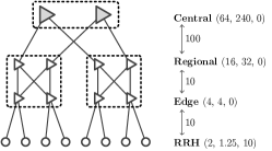
Figure 5: Description of a $k$-ary fat-tree infrastructure network with $k=2$; Nodes provide a given amount of computing $a_{\textrm{c}}$, memory $a_{\textrm{m}}$, and wireless $a_{\textrm{w}}$ resources expressed in number of used CPUs, Gbytes, and Gbps; Links are able to transmit data at a rate $a_{\text{b}}$ expressed in Gbps.

VI-A2 Background Services

At each infrastructure node $i\in\mathcal{N}$ and link $ij\in\mathcal{E}$, the resources consumed by best-effort background services follow a normal distribution with mean and standard deviation equal to respectively $20\,\%$ and $5\,\%$ percent of the available resource at that node and link, i.e., $\mu_{\text{B},n}\left(i\right)=0.2a_{n}\left(i\right)$, $\sigma_{\text{B},n}\left(i\right)=0.05a_{n}\left(i\right)$, $\forall i\in\mathcal{N}$, $\forall n\in\left\{\text{c},\text{m,\text{w}}\right\}$, and $\mu_{\text{B},\text{b}}\left(ij\right)=0.2a_{\text{b}}\left(ij\right)$, $\sigma_{\text{B},\text{b}}\left(ij\right)=0.05a_{\text{b}}\left(ij\right)$, $\forall ij\in\mathcal{E}$.

VI-A3 Slice Resource Demand (S-RD)

Three types of slices are considered.

• Slices of type 1 aim to provide an HD video streaming service at average rate of$4$ Mbps for VIP users, e.g., in a stadium. The number of users follows a binomial distribution $\mathcal{B}\left(300,0.9\right)$;

• Slices of type 2 are dedicated to provide an SD video streaming service at average rate of $2$ Mbps. The number of users follows a binomial distribution $\mathcal{B}\left(1000,0.8\right)$;

• Slices of type 3 aim to provide a video surveillance and traffic monitoring service at average rate of $1$ Mbps for $100$ cameras, e.g., installed along a highway.

The first two slice types address a video streaming service, and thus have the same function architecture with $3$ virtual functions: a virtual Video Optimization Controller (vVOC), a virtual Gateway (vGW), and a virtual Base Band Unit (vBBU). The third slice type consists of five virtual functions: a vBBU, a vGW, a virtual Traffic Monitor (vTM), a vVOC, and a virtual Intrusion Detection Prevention System (vIDPS).

As detailed in Section III-B, the resource requirements for the various SFCs that will have to be deployed within a slice are aggregated within an S-RD graph that mimics the SFC-RD graph. S-RD nodes and links are characterized by the aggregated resource needed to support the targeted number of users. Details of each resource type as well as the associated U-RD, SFC-RD, and S-RD graph are given in Table IV. Numerical values in Table IV have been adapted from [26].

VI-B Results

This section illustrates the performance of the four resource provisioning variants ($\mathtt{JP}$, $\mathtt{SP}$, $\mathtt{JP\text{-}B}$, and $\mathtt{SP\text{-}B}$), in terms of: utilization of infrastructure nodes and links, maximal probability of impact $p^{\text{im}}$ on the background services at every infrastructure node and link, provisioning cost, total earnings of the InP, and the number of impacted nodes and links, i.e., the number of nodes $i\in\mathcal{N}$ such that $\exists n\in\left\{\text{c},\text{m},\text{w}\right\}$ $p_{n}^{\text{im}}\left(i\right)>\overline{p}^{\text{im}}$ and links $ij\in\mathcal{E}$ such that $p_{\text{b}}^{\text{im}}\left(ij\right)>\overline{p}^{\text{im}}$.

VI-B1 Provisioning of a Single Slice

Table II shows the performance of two variants $\mathtt{SP\text{-}B}$ and $\mathtt{SP}$ for the provisioning of a single slice of Type 1, where $\underline{p}_{s}=0.99$ and $\overline{p}^{\text{im}}=0.1$. It is observed that the $\mathtt{SP}$ variant, which does not account for impact on background services, has a lower link usage and provisioning cost, and yields a higher earning for the InP than that of the $\mathtt{SP\text{-}B}$ variant. Nevertheless, as expected, the $\mathtt{SP}$ variant has a higher impact on background services, with maximal impact probability of $0.58$ exceeding the maximum tolerated impact probability $\overline{p}^{\text{im}}$ at one infrastructure node, as summarized in Table II.

TABLE II: Performance of $\mathtt{SP\text{-}B}$ and $\mathtt{SP}$ on Single Slice Provisioning

Criteria	$\mathtt{SP\text{-}B}$	$\mathtt{SP}$
Node usage	$33\%$	$33\%$
Link usage	$28\%$	$25\%$
Maximal $p^{\text{im}}$	$1.26\text{e-}4$	$0.58$
Provisioning cost	$332$	$326$
Total earnings	$568$	$574$
#impacted nodes	$0$	$1$
#impacted links	$0$	$0$

The way $\overline{p}^{\text{im}}$ affects the performance of $\mathtt{SP\text{-}B}$ is shown in Figures 6a-6d, when $\underline{p}_{s}=0.99$ and $\overline{p}^{\text{im}}$ ranges from $0.05$ to $0.4$. One observes that, the higher $\overline{p}^{\text{im}}$, the lower the provisioning cost and the higher earnings for the InP. This is due to the fact that, with higher $\overline{p}^{\text{im}}$, it is easier to provision slices with limited resources. This can be observed in the decrease of link usage in Figure 6c. On the other hand, the impact probability $p^{\text{im}}$ is always kept under the threshold $\overline{p}^{\text{im}}$ imposed by the InP, as shown in Figure 6d.

(a) Provisioning cost

(b) Total earnings

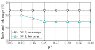
(c) Node and link usage

(d) Evolution of $p^{\text{im}}$ as a function of $\overline{p}^{\text{im}}$

Figure 6: Performance of the $\mathtt{SP\text{-}B}$ approach on single slice provisioning problem with different values of $\overline{p}^{\text{im}}$, in terms of (a) provisioning cost, (b) total earnings, (c) node and link utilization, and (d) maximal impact probability $p^{\text{im}}$.

VI-B2 Provisioning Several Slices of the Same Type

Now, considering $10$ slices of type $1$ with the same $\underline{p}_{s}=0.99$ , the $\mathtt{SP\text{-}B}$ and $\mathtt{SP}$ variants are compared in terms of acceptance rate, i.e., percentage of slices that have been successfully provisioned, given by $\sum_{s\in\mathcal{S}}\frac{x_{s}}{\left|\mathcal{S}\right|}$, for different value of $\underline{p}_{s}$, see Figure 7a. The tolerated impact probability $\overline{p}^{\text{im}}$ is set to $0.1$. As expected, when $\underline{p}_{s}$ increases, the acceptance rate decreases. Moreover, the $\mathtt{SP}$ approach, which does not account for background services, has always a higher acceptance rate compared to the $\mathtt{SP\text{-}B}$ approach.

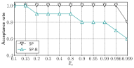
(a) Acceptance rate

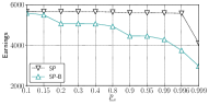
(b) Total earnings

Figure 7: Performance of the $\mathtt{SP\text{-}B}$ and $\mathtt{SP}$ approaches on the provisioning of multiple slices of one type, with different values of $\underline{p}_{s}$, in terms of (a) acceptance rate and (b) total earnings.

VI-B3 Provisioning of Several Slices of Different Types

The performance of the four variants is illustrated in this section, when resources of $2$ to $8$ slices of three different types have to be provisioned. The number of slices of each type and their associated $\underline{p}_{s}$ are detailed in Table III. The impact probability threshold $\overline{p}^{\text{im}}$ is set to $0.1$ in all scenarios.

TABLE III: Number of slices of each type as a function of $|\mathcal{S}|$

Case	#Type 1	#Type 2	#Type 3
$|\mathcal{S}|=2$	$1$	$1$	$0$
$|\mathcal{S}|=4$	$2$	$1$	$1$
$|\mathcal{S}|=6$	$2$	$2$	$2$
$|\mathcal{S}|=8$	$3$	$2$	$3$

The use of infrastructure nodes and links is shown in Figures 8a and 8b. The joint provisioning approaches ($\mathtt{JP}$ and $\mathtt{JP\text{-}B}$) require a reduced amount of nodes and links compared to the sequential schemes ($\mathtt{SP}$ and $\mathtt{SP\text{-}B}$). Moreover, considering the impact on background services requires, again, provisioning resources on more nodes and links.

Figure 8c shows the provisioning costs obtained with the various approaches. One observes that the $\mathtt{JP}$ variant yields the smallest cost among all variants, as it aims at finding an optimal solution for all slices, without considering the impact probability, contrary to the $\mathtt{JP\text{-}B}$ variant. This leads to the highest earnings for the InP, as shown in Figure 8d.

The total number of impacted nodes and links is shown in Figure 8e. The $\mathtt{JP\text{-}B}$ and $\mathtt{SP\text{-}B}$ variant have no impacted nodes or links, whereas the provisioning performed by the $\mathtt{JP}$ and $\mathtt{SP}$ approaches significantly impact the background services. The $\mathtt{SP}$ variant has a higher impact on the background services, due to the higher utilization of infrastructure nodes and links, as shown in Figures 8a and 8b.

From the InP perspective, the use of impact-unaware variants ($\mathtt{JP}$ and $\mathtt{SP}$) maximizes its earning but violates background services at a significant number of infrastructure nodes and links. This may necessitate to reconfigure those background services. On contrary, by using the impact-aware variants ($\mathtt{JP\text{-}B}$ and $\mathtt{SP\text{-}B}$), the InP can provision slices and preserve a tolerable impact on the background services. The price to be paid is somewhat degraded node and link utilization efficiency and a higher provisioning cost compare to the impact-aware variants, leading to a lower earnings for the InP. For instance, when provisioning for $4$ slices, the $\mathtt{JP\text{-}B}$ variant uses around $72\%$ of the total infrastructure nodes to aggregate resources needed to support the slices, while only $66.7\%$ of the nodes are employed by the $\mathtt{JP}$ method, leading to a reduction of $3.5\%$ of total earnings, as depicted in Figures 8a and 8d.

As expected, the sequential provisioning methods ($\mathtt{SP\text{-}B}$ and $\mathtt{SP}$) perform better in terms of computing time than the joint approaches ($\mathtt{JP\text{-}B}$ and $\mathtt{JP}$). Increasing the number of slices leads to an increase of the cardinality of the sets of variables $\boldsymbol{d}$ and $\boldsymbol{\kappa}$, and therefore increases the computing time. In sequential provisioning, slices are considered successively. There is only a very small difference (usually less than $5\%$) in computing time between the $\mathtt{SP\text{-}B}$ and $\mathtt{SP}$ approaches and between the $\mathtt{JP\text{-}B}$ and $\mathtt{JP}$ approaches.

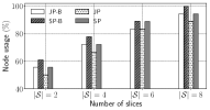
(a)

(b)

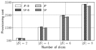
(c)

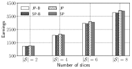
(d)

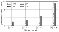
(e)

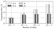
(f)

Figure 8: Performance comparison of $4$ variants in terms of utilization of infrastructure nodes (a), infrastructure links (b), provisioning costs (c), total earnings (d), number of impacted nodes and links (e), and computing time (f).

TABLE IV: Parameters of U-RD, SFC-RD, and S-RD graphs

Type 1: HD video streaming at $4$ Mbps. $N_{s}\sim\mathcal{B}\left(300,0.9\right)$, $I_{s}=900$, $\underline{p}_{s}=0.99$
Node	$\left(\mu_{s,\text{c}},\sigma_{s,\text{c}}\right)$	$\left(\mu_{s,\text{m}},\sigma_{s,\text{m}}\right)$	$\left(\mu_{s,\text{w}},\sigma_{s,\text{w}}\right)$	$\left(r_{\text{c}},r_{\text{m}},r_{\text{w}}\right)$		Link	$\left(\mu_{\text{b}},\sigma_{\text{b}}\right)$	$r_{s,\text{b}}$
vVOC	$\left(5.4,0.54\right)\textrm{e-}3$	$\left(1.5,0.15\right)\textrm{e-}2$	—	$\left(0.29,0.81,0\right)$		vVOC$\rightarrow$vGW	$\left(4,0.4\right)\textrm{e-}3$	$0.22$
vGW	$\left(9.0,0.90\right)\textrm{e-}4$	$\left(5.0,0.50\right)\textrm{e-}4$	—	$\left(0.05,0.03,0\right)$		vGW$\rightarrow$vBBU	$\left(4,0.4\right)\textrm{e-}3$	$0.22$
vBBU	$\left(8.0,0.80\right)\textrm{e-}4$	$\left(5.0,0.50\right)\textrm{e-}4$	$\left(4,0.4\right)\textrm{e-}3$	$\left(0.04,0.03,0.2\right)$
Type 2: SD video streaming at $2$ Mbps. $N_{s}\sim\mathcal{B}\left(1000,0.8\right)$, $I_{s}=1000$, $\underline{p}_{s}=0.95$
Node	$\left(\mu_{s,\text{c}},\sigma_{s,\text{c}}\right)$	$\left(\mu_{s,\text{m}},\sigma_{s,\text{m}}\right)$	$\left(\mu_{s,\text{w}},\sigma_{s,\text{w}}\right)$	$\left(r_{\text{c}},r_{\text{m}},r_{\text{w}}\right)$		Link	$\left(\mu_{\text{b}},\sigma_{\text{b}}\right)$	$r_{s,\text{b}}$
vVOC	$\left(1.1,0.11\right)\textrm{e-}3$	$\left(7.5,0.75\right)\textrm{e-}3$	—	$\left(0.17,1.20,0\right)$		vVOC$\rightarrow$vGW	$\left(2,0.2\right)\textrm{e-}3$	$0.32$
vGW	$\left(1.8,0.18\right)\textrm{e-}4$	$\left(2.5,0.25\right)\textrm{e-}4$	—	$\left(0.03,0.04,0\right)$		vGW$\rightarrow$vBBU	$\left(2,0.2\right)\textrm{e-}3$	$0.32$
vBBU	$\left(0.8,0.08\right)\textrm{e-}4$	$\left(2.5,0.25\right)\textrm{e-}4$	$\left(2,0.2\right)\textrm{e-}3$	$\left(0.01,0.04,0.3\right)$
Type 3: Video surveillance and traffic monitoring at $1$ Mbps. $N_{s}=50$, $I_{s}=800$, $\underline{p}_{s}=0.9$
Node	$\left(\mu_{s,\text{c}},\sigma_{s,\text{c}}\right)$	$\left(\mu_{s,\text{m}},\sigma_{s,\text{m}}\right)$	$\left(\mu_{s,\text{w}},\sigma_{s,\text{w}}\right)$	$\left(r_{\text{c}},r_{\text{m}},r_{\text{w}}\right)$		Link	$\left(\mu_{\text{b}},\sigma_{\text{b}}\right)$	$r_{s,\text{b}}$
vBBU	$\left(2.0,0.20\right)\textrm{e-}4$	$\left(1.3,0.13\right)\textrm{e-}4$	$\left(1,0.1\right)\textrm{e-}3$	$\left(0.4,0.25,2\right)\textrm{e-}2$		vBBU$\rightarrow$vGW	$\left(1,0.1\right)\textrm{e-}3$	$0.02$
vGW	$\left(9.0,0.90\right)\textrm{e-}4$	$\left(1.3,0.13\right)\textrm{e-}4$	—	$\left(0.018,0.003,0\right)$		vGW$\rightarrow$vTM	$\left(1,0.1\right)\textrm{e-}3$	$0.02$
vTM	$\left(1.1,0.11\right)\textrm{e-}3$	$\left(1.3,0.13\right)\textrm{e-}4$	—	$\left(0.266,0.003,0\right)$		vTM$\rightarrow$vVOC	$\left(1,0.1\right)\textrm{e-}3$	$0.02$
vVOC	$\left(5.4,0.54\right)\textrm{e-}3$	$\left(3.8,0.38\right)\textrm{e-}3$	—	$\left(0.108,0.080,0\right)$		vVOC$\rightarrow$vIDPS	$\left(1,0.1\right)\textrm{e-}3$	$0.02$
vIDPS	$\left(1.1,0.11\right)\textrm{e-}2$	$\left(1.3,0.13\right)\textrm{e-}4$	—	$\left(0.214,0.003,0\right)$

VII Conclusions

This paper investigates a resource provisioning method for network slicing robust to a partly unknown number of users whose resource demands are uncertain. Adopting the point of view of the InP, one tries to maximize its earnings, while providing a probabilistic guarantee that the slice resource demands are fulfilled. In addition to that, the proposed resource provisioning method is performed to keep the impact on the background services under a threshold imposed by the InP.

The uncertainty-aware slice resource provisioning is formulated as a nonlinear constrained optimization problem. A parameterized MILP formulation is then proposed. With the MILP formulation, four variants ($\mathtt{JP}$, $\mathtt{SP}$, $\mathtt{JP\text{-}B}$, and $\mathtt{SP\text{-}B}$) are introduced, for the solution of the provisioning problem for multiple slices jointly or sequentially, without or with consideration of the impact on background services.

The impact-limiting variants ($\mathtt{JP\text{-}B}$, and $\mathtt{SP\text{-}B}$) have a controlled impact on the background services, whereas the $\mathtt{JP}$ and $\mathtt{SP}$ variants, which do not care of the impact on background services, consume all resources of several infrastructure nodes and links, which may impose a reconfiguration of background services. The price to be paid for the InP with impact-limiting variants are lower earnings.

Moreover, due to the exponential worst-case complexity in the number of variables of the MILP formulation, as expected, sequential approaches are shown to better scale to a larger number of slices. The price to be paid by the sequential approaches is a somewhat degraded node and link utilization, a higher provisioning cost, and lower earnings, compared to the joint approaches.

In this paper, uncertainties related to the fluctuation of user demands and the background services have been taken into account for the slice resource provisioning. A prospective extension to this work is to let the InP, if necessary, update the already provisioned resources for some slices during their lifetime. This allows one to have a more realistic adaptive SLAs and dynamic provisioning techniques for network slicing.

References

- [1] 5G Americas, “Network Slicing for 5G and Beyond,” White Paper, 2016.
- [2] IETF, “Network Slicing Architecture,” Internet-Draft, pp. 1–8, 2017.
- [3] A. A. Barakabitze, A. Ahmad, R. Mijumbi, and A. Hines, “5G Network Slicing Using SDN and NFV: A Survey Of Taxonomy, Architectures And Future Challenges,” Computer Networks, vol. 167, 2020.
- [4] C. Liang and F. R. Yu, “Wireless Network Virtualization: A Survey, Some Research Issues and Challenges,” IEEE Commun. Surveys Tuts., pp. 1–24, 2014.
- [5] P. Rost, C. Mannweiler, D. S. Michalopoulos, C. Sartori, V. Sciancalepore, N. Sastry, O. Holland, S. Tayade, B. Han, D. Bega, D. Aziz, and H. Bakker, “Network Slicing to Enable Scalability and Flexibility in 5G Mobile Networks,” in IEEE Commun. Mag., vol. 55, no. 5, 2017, pp. 72–79.
- [6] GSM Alliance, “An Introduction to Network Slicing,” White Paper, 2017.
- [7] M. Richart, J. Baliosian, J. Serrat, and J. L. Gorricho, “Resource Slicing in Virtual Wireless Networks: A Survey,” IEEE Trans. Netw. Service Manag., vol. 13, no. 3, pp. 462–476, 2016.
- [8] N. Huin, B. Jaumard, and F. Giroire, “Optimization of Network Service Chain Provisioning,” in Proc. IEEE ICC, 2017.
- [9] G. Wang, G. Feng, W. Tan, S. Qin, W. Ruihan, and S. Sun, “Resource Allocation for Network Slices in 5G with Network Resource Pricing,” in Proc. IEEE GLOBECOM, 2017, pp. 1–6.
- [10] R. Su, D. Zhang, R. Venkatesan, Z. Gong, C. Li, F. Ding, F. Jiang, and Z. Zhu, “Resource Allocation for Network Slicing in 5G Telecommunication Networks: A Survey of Principles and Models,” IEEE Network, vol. 33, no. 6, pp. 172–179, 2019.
- [11] T. Trinh, H. Esaki, and C. Aswakul, “Quality of Service Using Careful Overbooking for Optimal Virtual Network Resource Allocation,” in Proc. ECTI, 2011, pp. 296–299.
- [12] S. Coniglio, A. M. Koster, and M. Tieves, “Virtual Network Embedding Under Uncertainty: Exact And Heuristic Approaches,” in Proc. DRCN. IEEE, 2015, pp. 1–8.
- [13] S. Mireslami, L. Rakai, M. Wang, and B. H. Far, “Dynamic Cloud Resource Allocation Considering Demand Uncertainty,” IEEE Trans. on Cloud Comput., vol. 7161, no. c, pp. 1–1, 2019.
- [14] A. Fendt, C. Mannweiler, L. C. Schmelz, and B. Bauer, “An Efficient Model for Mobile Network Slice Embedding under Resource Uncertainty,” in Proc. ISWCS, 2019, pp. 602–606.
- [15] A. Baumgartner, T. Bauschert, F. D’Andreagiovanni, and V. S. Reddy, “Towards Robust Network Slice Design under Correlated Demand Uncertainties,” in Proc. ICC, 2018, pp. 1–7A.
- [16] D. Bertsimas and M. Sim, “Robust Discrete Optimization and Network Flows,” Mathematical Programming, vol. 98, no. 1-3, pp. 49–71, 2003.
- [17] T. Bauschert and V. S. Reddy, “Genetic Algorithms for the Network Slice Design Problem Under Uncertainty,” in Proc. GECCO Companion, 2019, pp. 360–361.
- [18] R. Wen, G. Feng, J. Tang, T. Q. Quek, G. Wang, W. Tan, and S. Qin, “On Robustness of Network Slicing for Next-Generation Mobile Networks,” IEEE Trans. Commun., vol. 67, no. 1, pp. 430–444, 2019.
- [19] R. Riggio, A. Bradai, D. Harutyunyan, T. Rasheed, and T. Ahmed, “Scheduling Wireless Virtual Networks Functions,” IEEE Trans. Netw. Service Manag., vol. 13, no. 2, pp. 240–252, 2016.
- [20] P. Vizarreta, M. Condoluci, C. M. Machuca, T. Mahmoodi, and W. Kellerer, “QoS-driven Function Placement Reducing Expenditures in NFV Deployments,” in Proc. IEEE ICC, 2017.
- [21] Q.-T. Luu, S. Kerboeuf, A. Mouradian, and M. Kieffer, “A Coverage-Aware Resource Provisioning Method for Network Slicing,” to appear in IEEE/ACM Trans. Netw., pp. 1–14, 2020, arXiv:1907.09211 [cs.NI].
- [22] J. Wang, K. L. Wright, and K. Gopalan, “XenLoop: A Transparent High Performance Inter-VM Network Loopback,” Cluster Comput., vol. 12, no. 2 SPEC. ISS., pp. 141–152, 2009.
- [23] C. Jiang, G. Han, J. Lin, G. Jia, W. Shi, and J. Wan, “Characteristics of Co-Allocated Online Services and Batch Jobs in Internet Data Centers: A Case Study from Alibaba Cloud,” IEEE Access, vol. 7, pp. 22 495–22 508, 2019.
- [24] A. Genz, “Numerical Computation of Rectangular Bivariate and Trivariate Normal and t Probabilities,” Statistics and Computing, vol. 14, no. 3, pp. 251–260, 2004.
- [25] N. Bouten, R. Mijumbi, J. Serrat, J. Famaey, S. Latre, and F. De Turck, “Semantically Enhanced Mapping Algorithm for Affinity-Constrained Service Function Chain Requests,” IEEE Trans. Netw. Service Manag., vol. 14, no. 2, pp. 317–331, 2017.
- [26] M. Savi, M. Tornatore, and G. Verticale, “Impact of Processing-Resource Sharing on the Placement of Chained Virtual Network Functions,” in Proc. IEEE NFV-SDN, 2016, pp. 191–197.