Deflection Angle and Shadow Behaviors of Quintessential Black Holes in arbitrary Dimensions

Abstract

Motivated by M-theory/superstring inspired models, we investigate certain behaviors of the deflection angle and the shadow geometrical shapes of higher dimensional quintessential black holes associated with two values of the dark energy (DE) state parameter, being $\omega=-\frac{1}{3}$ and $\omega=-\frac{2}{3}$. Concretely, we derive the geodesic equation of photons on such backgrounds. Thanks to the Gauss-Bonnet theorem corresponding to the optical metric, we compute the leading terms of the deflection angle in the so-called weak-limit approximation. After that, we inspect the effect of DE and the space-time dimension $d$ on the calculated optical quantities. Introducing DE via the field intensity $c$ and the state parameter $\omega$, we find that the shadow size and the deflection angle increase by increasing values of the field intensity $c$. However, we observe that the high dimensions decrease such quantities for $\omega$-models exhibiting similar behaviors. Then, we consider the effect of the black hole charge, on these optical quantities, by discussing the associated behaviors. The present investigation recovers certain known results appearing in ordinary four dimensional models.

Keywords: Higher dimensional black holes, Quintessential dark energy, Shadow, Deflection angle.

1 Introduction

Recently, after the successful observation of the first image of the black hole in the electromagnetic spectrum in the center of galaxy M87 [1, 2], there is a continuous improvement of measurements for much higher resolution in the future [3], since a clear geometrical identification of the black hole from the first image is not allowed. Subsequently, it is hard to put aside the theoretical efforts dealing with the black hole physics in diverse gravitational theories and astrophysical mediums.

Black holes involve the natural peculiarity of sucking in surrounding matter in a phenomenon called ”accretion”. This matter, accrediting on the black hole, passes through the horizon. It has been observed that this gives a dark area on a light background called the ”shadow” of the black hole being based on the so-called gravitational lensing phenomenon. It turns out that the shape and the size of the light generated by matter, flowing at the edge of the event horizon, can be determined by the black hole parameters including the mass and rotation [4]. For non-rotating black holes, it has been found that the shape of the shadow develops a circular geometry. However, rotating black holes involve non trivial shapes depending on the rotation parameter [5]. Various black hole models, in arbitrary dimensions, have been investigated using different methods and approaches including supergravity theories [6]. These activities have been motivated by string theory requiring more than four physical directions. In fact, the first successful numerical counting of the entropy of black-hole in such a non-trivial theory was performed in five-dimensional space-time unveiling the microscopic stringy description of black holes [7, 8]. Moreover, several efforts have been deployed to test extra dimensions in future colliders, where the study of higher-dimensional black holes properties could take place. In particular, the investigation of the presence of extra dimensions greatly could suggest a new physics dealing with higher dimensional black holes. It is expected that this could be experimentally accessible and manifests itself through a number of strong gravity effects, as soon as the energy of a given experiment exceeds some characterising fundamental scale under the the four-dimensional Planck scale. The Large Hadron Collider (LHC) at CERN, with a center-of-mass energy of 14 TeV, becomes then a natural place to look for such extra dimensions as well as strong gravity effects which could be associated with such black holes. Indeed, the latters, might be detected via their radiation spectra according to the evaporation process along with an additional number of distinct observable signatures, which could support the existence of these extra dimensions. The presence of such hidden dimensions has became a primordial element in the comprehension of unified theories including string/M-theory inspired models. This could suggest that there can be some remnants of the extra dimensions in the detection of the gravitational waves, encoding some information associated with the underling size and the dynamics of fluctuations modes. In this way, many works have been elaborated to unveil such a physics [9, 10, 11, 12]. Despite many attempts to support such activities, it has not been successful up to now. Nowadays, thanks to EHT, we dispose of new tools to continue hunting of the hidden dimensions [13]. However, in order to understand the observed black hole shadow, gravitational lensing can be a helpful instrument of astrophysics and astronomy [14, 15]. Precisely, the discovery of dark matter filaments with the help of the weak deflection is an extremely relevant topic since it is very helpful in the investigation of the Universe structure [16, 17, 18, 19, 20, 21, 22, 23].

Besides, it is now widely supposed that only 5% of mass and energy in the universe is visible and it is well described within the standard model of particle physics [24]. While, the remaining large hidden part consists of 25% of dark matter and 70% of dark energy (DE), whose the existence and the nature are still undetermined [25, 26]. The supposed existence of dark matter is highly motivated by the non-Newtonian behavior of high velocities of stars at the outskirts of galaxies. This might imply that visible disks of galaxies are flooded in a much larger, roughly spherical, halo of invisible matter [27, 28]. For DE, affecting the universe on the largest scales, the first observational proof for its existence arose from supernovae measurements. Namely, distant Ia-type supernova explosions point out that a very small repulsive cosmological constant, i.e., vacuum energy, quintessential field, manifesting repulsive gravitational effect, are needful for the explanation of the accelerated expansion of the recent Universe [29, 30]. Similar motivations in favor of DE are also concluded by the Planck space observatory measurements of the cosmic microwave background [31].

Since the role of the vacuum energy has been widely discussed in cosmological models [32, 34, 33], thus, it is also pertinent to consider its role in the physical processes taking place near black holes, essentially in the vicinity of the black hole horizon [35]. More recently, the physics of black holes in the presence of such an energy has been extensively developed. Precisely, a special emphasis has put on quintessential black holes from M-theory/superstring inspired models [36].

The aim of this work is to contribute to these activities by investigating certain optical behaviors of higher dimensional quintessential black hole (QBH) and estimating the energy emission rate associated with two values of the DE state parameter being $\omega=-\frac{1}{3}$ and $\omega=-\frac{2}{3}$. Concretely, we get the geodesic equations of photons on such backgrounds. Using the Gauss-Bonnet theorem associated with the optical metric, we calculate the leading terms of the deflection angle in the weak-limit approximation framework. Varying the space-time dimension $d$ and introducing DE via the field intensity $c$ and the state parameter $\omega$, we find that the shadow size and the deflection angle increase within increasing values of the field intensity $c$. However, it has been shown that the higher dimensions decrease such quantities for $\omega$-models revealing similar behaviors. Then, we study the effect of the black hole charge on such computed optical quantities. The present investigation, which recovers some known four dimensional ordinary results, comes up with certain open questions associated with M-theory/superstring inspired models where DE could find a possible place supported by extra dimensions.

The paper is organized as follows. In section 2, we reconsider the study of the non-charged Schwarzschild-Tangherlini solutions in higher dimensions with the presence of quintessential DE. In particular, we investigate the effective potential and the shadow geometrical behaviors of such a QBH. In section 3, we compute and graphically analyse, in some details, the significant impact of the quintessential energy on the Shwarzschild-Tanglerlini black hole deflection angle. In this section 4, we study the effect of the charge of Schwarzschild-Tangherlini holes on such optical quantities. The section 5 is devoted to the discussion on possible extensions, the summary of the work, and certain open questions. Some used material associated with the metric calculations are given in the appendix.

2 Shadow behaviors of Quintessential Schwarzschild-Tangherlini black hole

In this section, we reconsider the investigation of quintessential Schwarzschild-Tangherlini black holes [37]. Before going ahead, it is now known that the general properties of the universe are described by assuming that its dynamics are ruled by an energy source, i.e., DE, whose the physical origin remains unknown. This cosmological component has an energy-momentum tensor which can be obtained from Friedmann’s equations. A remarkable characteristic of this antigravitational energy component is its negative pressure which is comparable, in absolute value, to the energy density. Therefore, whatever its nature is, DE can be effectively depicted in terms of the pressure and the density. Treated as a perfect fluid with pressure $p$ and energy density $\mathbf{\rho}$, a parametrization of DE is possible via the introduction of what is known as the equation of state parameter, being the ratio of its pressure and density

$$\omega=\frac{p}{\mathbf{\rho}}.$$ (2.1)

From such an equation of the state, some of the well studied cases of fluids are

• $\omega=-1$ associated with the cosmological constant $\Lambda$,

• $\omega=0$ corresponding to a pressureless regime like non-relativistic matter, i.e., dust

• $\omega=1/3$ associated with a radiation.

For a repulsive gravity effect, it appears that, in a homogeneous and isotropic universe, the corresponding fluid equation of state is $\omega<-1/3$. Therefore, the cosmological constant $\Lambda$, or any fluid with equation of state $\omega<-1/3$ accelerates the expansion. One of such a hypothetical DE fluid is the quintessence. The latter is a dynamical, evolving, spatially inhomogeneous component (unlike a cosmological constant, its pressure and energy density evolve in time). Thus, $\omega$ may also do so with equation of state $-1<\omega<0.$ The smaller is the value of $\omega$, the greater its accelerating effect. Such a dynamical DE field which is thought to drive the overall cosmic history of the universe, may also still affect its large structure, for instance, galaxies, black holes including their thermodynamical and optical aspects.
In connections with gravity models, there has been a significant interest in the study of higher dimensional of Einstein equations providing black hole solutions considered as the most exact ones of general relativity. Such solutions could encourage the black hole buildings from string theory involving more than four dimensions. Such higher dimensional solutions, which will be dealt with, could be supported by the physics of extra dimensions being a possible investigation subject within future colliders including LHC. Motivated by such activities, we would like to study the shadow of the black hole in arbitrary dimensions.

According to [38], the line element of the metric, in higher dimensional space-times with static black holes, takes the following form

$$ds^{2}=-e^{\nu}dt^{2}+e^{\lambda}dr^{2}+r^{2}d\Omega^{2}_{d-2},$$ (2.2)

where $d\Omega^{2}_{d-2}=d\theta^{2}_{1}+\sin^{2}\theta_{1}^{2}d\theta^{2}_{2}+\ldots+\prod^{d-3}_{i=1}\sin^{2}\theta_{i}d\theta^{2}_{d-2}$ represents the metric on the $(d-2)$-dimensional unit sphere. It is noted that $\nu$ and $\lambda$ are two functions of the radial coordinate $r$, respectively. In the static spherically symmetric state, in presence of the quintessence, the the energy-momentum tensor can be written as [35]

$${T_{t}}^{t}=A(r),\qquad{T_{t}}^{j}=0,\qquad{T_{i}}^{j}=C(r)\,r_{i}\,r^{j}+B(r)\,{\delta_{i}}^{j}.$$ (2.3)

The average angle of the isotropic state provides

$${\langle{T_{i}}^{j}\rangle=D(r)\,{\delta_{i}}^{j},}\qquad{D(r)=-\frac{1}{d-1}\,C(r)\,r^{2}+B(r).}$$ (2.4)

For the quintessence, one has the solution

$${D(r)=-w_{q}\,A(r)}$$ (2.5)

where $A(r)$ is a density term. It is recalled that, for a fixed state parameter $\omega$, we can get the expression of $D(r)$. $C(r)\equiv 0$ represents the condition associated with a free quintessence [35]. Taking the metric Eq.(2.2) and applying the calculations given in the appendix, we obtain Einstein’s equation. Indeed, the involved terms are

$${2T_{t}^{\;t}}\; = {\frac{(d-2)e^{-\lambda}\left((d-3)\left(e^{\lambda}-1\right)+r\lambda^{\prime}\right)}{2r^{2}},}$$ (2.6)

$${2T_{r}^{\;r}}\; = \;{\frac{(d-2)e^{-\lambda}\left((d-3)\left(e^{\lambda}-1\right)-r\nu^{\prime}\right)}{2r^{2}},}$$ (2.7)

$${2T_{\theta_{i}}^{\;\theta_{i}}}\; = \;{-\frac{e^{-\lambda}\left(2(d-3)r\left(\nu^{\prime}-\lambda^{\prime}\right)+2(d-4)(d-3)-r^{2}\lambda^{\prime}\nu^{\prime}+2r^{2}\nu^{\prime\prime}+r^{2}\left(\nu^{\prime}\right)^{2}\right)}{4r^{2}}}$$ (2.8)

$$+ {\frac{(d-3)(d-4)}{2r^{2}}}\hskip 28.45274pt{i=1,\ldots,d-2,}$$ (2.9)

where the prime represent the derivative with respect to $r$. In a higher dimensional spherically-symmetric space-time, the general expression of the energy-momentum tensor in the presence of the quintessence reads as

$${{T_{t}}^{t}}={\rho_{q}(r),}$$ (2.10)

$${{T_{i}}^{j}}={\rho_{q}(r)\,\alpha\left[-(1+(d-1)\,B)\frac{r_{i}\,r^{j}}{r_{n}r^{n}}+B\,{\delta_{i}}^{j}\right]}.$$ (2.11)

It is noted that there is a proportionality between the spatial components and the temporal one with the arbitrary parameter $B$ depending on the internal structure of the quintessence. Considering $\langle r_{i}\,r^{j}\rangle=\frac{1}{d-1}\,{\delta_{i}}^{j}\,r_{n}r^{n}$, the isotropic average over the angle results is given by

$$\left\langle{{T_{i}}^{j}}\right\rangle={-\rho_{q}(r)\,\frac{\alpha}{d-1}\,{\delta_{i}}^{j}=-p_{q}(r)\,{\delta_{i}}^{j},}$$ (2.12)

Using Eq.(2.1), one has the constraint

$$w=\frac{\alpha}{d-1}.$$ (2.13)

Applying the principle of the additivity and the linearity, used in [35, 38], we get

$$\lambda=-\ln(f_{\omega}),$$ (2.14)

By the help of Eq.(2.14), one obtains the linear differential equations involving $f_{\omega}$

$${T_{t}^{\;t}} = {T_{r}^{\;r}}=-\frac{d-2}{2r^{2}}(rf^{\prime}_{\omega}+(d-3)(f_{\omega}-1)),$$ (2.15)

$${T_{\theta_{i}}^{\;\theta_{i}}} = {-\frac{1}{4r^{2}}(r^{2}f^{\prime\prime}_{\omega}+2(d-3)rf^{\prime}_{\omega}+(d-4)(d-3)(f_{\omega}-1)),}\quad{i=1,\ldots,d-2.}$$ (2.16)

Combining equations Eq.(2.10), Eq.(2.11) and Eq.(2.15), one can find the fixed parameter $B$ given by

$${B=-\frac{(d-1)\omega+1}{(d-1)(d-2)\omega}}.$$ (2.17)

The energy-momentum tensor, appearing in Eq.(2.11), takes the following form

$${T_{t}^{\;t}} = {T_{r}^{\;r}}={\color[rgb]{1,0,0}\rho,}$$ (2.18)

$${T_{\theta_{i}}^{\;\theta_{i}}} = {-\frac{1}{d-2}(1+\omega(d-1)),}\quad{i=1,\ldots,d-2,.}$$ (2.19)

From Eq.(2.15), Eq.(2.16), Eq.(2.18) and Eq.(2.19), we get a differential equation for $f$

$${r^{2}f^{\prime\prime}_{\omega}+(d(\omega+2)-(\omega+5))rf^{\prime}_{\omega}+(d-3)(f_{\omega}-1)(d(\omega+1)-(\omega+3))=0,}$$ (2.20)

providing a solution given by

$${f_{\omega}(r)=1-\frac{\mu}{r^{d-3}}-\frac{c}{r^{\omega(d-1)+d-3}},}$$ (2.21)

where $\mu$ and $c$ are normalization factors. The energy density $\rho$, given in Eq.(2.1), should be positive and take the following form

$${\rho=\frac{c(d-1)(d-2)\omega}{4r^{(d-1)(\omega+1)}}}.$$ (2.22)

The line element of the metric, in such a higher dimensional spherically symmetric black hole surrounded by the quintessence, reduces to

$${ds^{2}=-f_{\omega}(r)dt^{2}+\frac{1}{f_{\omega}(r)}dr^{2}+r^{2}d\Omega^{2}_{d-2}},$$ (2.23)

and $\mu$ is related to the black hole masse $M$ through the relation

$$\mu=\frac{16\pi M}{(d-2)\Omega_{d-2}},$$ (2.24)

where one has $\Omega_{d-2}=\frac{2\pi^{\frac{d-1}{2}}}{\Gamma(\frac{d-1}{2})}$. Roughly, the Lagrange and the Hamilton-Jacobi equation can be exploited to get the equations of motion generating QBH shadow geometric shapes using the following Lagrangian

$$\mathcal{L}=\frac{1}{2}g_{\mu\nu}\dot{x}^{\mu}\dot{x}^{\nu}.$$ (2.25)

The solution of the canonically conjugate momentums provides

$$\frac{dt}{d\tau}=\frac{E}{f_{\omega}(r)},\quad\frac{d\theta_{d-2}}{d\tau}=\frac{L}{r^{2}\prod_{i=1}^{d-3}\sin^{2}\theta_{i}},$$ (2.26)

where $\tau$ is the affine parameter along the geodesics. $E$ and $L$ are the energy and the angular momentum of the test particle, respectively. To get the shadow of the black hole, one needs first to obtain the geodesic form of such a particle. To reach that, the Hamilton-Jacobi equation and Carter constant separable method should be used, matching the rotating case[39, 40]. Indeed, the Hamilton-Jacobi equation is expressed as

$$\frac{\partial{S}}{\partial\tau}=-\frac{1}{2}g^{\mu\nu}\frac{\partial S}{\partial x^{\mu}}\frac{\partial S}{\partial x^{\nu}},$$ (2.27)

where $S$ is the action Jacobi. The separable solution allows one to express the action as follows

$$S=\frac{1}{2}m^{2}_{0}\tau-Et+L\theta_{D-2}+S_{r}(r)+\sum_{i=1}^{D-3}S_{\theta_{i}}(\theta_{i}),$$ (2.28)

where $m_{0}$ is the mass of the test particle. $S_{r}(r)$ and $S_{\theta_{i}}(\theta_{i})$ are function depending of $r$ and $\theta$, respectively. Considering a test photon particle, the calculation provides

$$\begin{split}0&=\bigg{\{}f_{\omega}(r)^{-1}\bigg{(}\frac{\partial S}{\partial t}\bigg{)}^{2}-f_{\omega}(r)\bigg{(}\frac{\partial S}{\partial r}\bigg{)}^{2}-\frac{1}{r^{2}\prod_{i=1}^{D-3}\sin^{2}\theta_{i}}\bigg{(}\frac{\partial S_{\theta_{D_{2}}}}{\partial\theta_{D-2}}\bigg{)}^{2}\bigg{\}}\\ &-\bigg{\{}\sum_{i=1}^{D-3}\frac{1}{r^{2}\prod_{n=1}^{i-1}\sin^{2}\theta_{n}}\bigg{(}\frac{\partial S_{\theta_{i}}}{\partial\theta_{i}}\bigg{)}^{2}\bigg{\}},\end{split}$$ (2.29)

In this way, the separability of the equation gives

$$\begin{split}0&=\bigg{\{}f_{\omega}(r)^{-1}\bigg{(}\frac{\partial S}{\partial t}\bigg{)}^{2}-f_{\omega}(r)\bigg{(}\frac{\partial S}{\partial r}\bigg{)}^{2}-\frac{1}{r^{2}}\Bigg{(}\frac{1}{\prod_{i=1}^{D-3}\sin^{2}\theta_{i}}\bigg{(}\frac{\partial S_{\theta_{D-2}}}{\partial\theta_{D-2}}\bigg{)}^{2}\\ &+\mathcal{K}-\bigg{(}\frac{\partial S_{\theta_{D-2}}}{\partial\theta_{D-2}}\bigg{)}^{2}\;\prod_{i=1}^{D-3}\cot^{2}\theta_{i}\Bigg{)}\bigg{\}}\\ &-\bigg{\{}\frac{1}{r^{2}}\Bigg{(}\sum_{i=1}^{D-3}\frac{1}{\prod_{n=1}^{i-1}\sin^{2}\theta_{n}}\bigg{(}\frac{\partial S_{\theta_{i}}}{\partial\theta_{i}}\bigg{)}^{2}-\mathcal{K}+\bigg{(}\frac{\partial S_{\theta_{D-2}}}{\partial\theta_{D-2}}\bigg{)}^{2}\;\prod_{i=1}^{D-3}\cot^{2}\theta_{i}\Bigg{)}\bigg{\}},\end{split}$$ (2.30)

where $\mathcal{K}$ is the Carter constant. Replacing $\Big{(}\frac{\partial S_{\theta_{D-2}}}{\partial\theta_{D-2}}\Big{)}$ and $\big{(}\frac{\partial S}{\partial t}\big{)}$ by theirs expressions and introducing $L$ and $E$, we obtain

$$\begin{split}0&=\bigg{\{}f_{\omega}(r)^{-1}E^{2}-f_{\omega}(r)\bigg{(}\frac{\partial S}{\partial r}\bigg{)}^{2}-\frac{1}{r^{2}}\Bigg{(}\frac{L^{2}}{\prod_{i=1}^{D-3}\sin^{2}\theta_{i}}+\mathcal{K}-\prod_{i=1}^{D-3}L^{2}\cot^{2}\theta_{i}\Bigg{)}\bigg{\}}\\ &-\bigg{\{}\frac{1}{r^{2}}\Bigg{(}\sum_{i=1}^{D-3}\frac{1}{\prod_{n=1}^{i-1}\sin^{2}\theta_{n}}\bigg{(}\frac{\partial S_{\theta_{i}}}{\partial\theta_{i}}\bigg{)}^{2}-\mathcal{K}+\prod_{i=1}^{D-3}L^{2}\cot^{2}\theta_{i}\Bigg{)}\bigg{\}},\end{split}$$ (2.31)

After simplifications, we obtain

$$r^{2}f_{\omega}(r)^{2}\bigg{(}\frac{\partial S}{\partial r}\bigg{)}^{2} = E^{2}r^{2}-f_{\omega}(r)(\mathcal{K}+L^{2})$$ (2.32)

$$\sum_{i=1}^{D-3}\frac{1}{\prod_{n=1}^{i-1}\sin^{2}\theta_{n}}\bigg{(}\frac{\partial S_{\theta_{i}}}{\partial\theta_{i}}\bigg{)}^{2} = \mathcal{K}-\prod_{i=1}^{D-3}L^{2}\cot^{2}\theta_{i}.$$ (2.33)

Exploiting (2.26), (2.32), (2.33) and the definition of canonically conjugate momentum, we obtain the complete equations of motion for photon ($m_{0}=0$) around the Schwarzschild-Tangherlini quintessential black hole

$$\frac{dt}{d\tau} = \frac{E}{f_{\omega}(r)}$$ (2.34)

$$r^{2}\frac{dr}{d\tau} = \pm\sqrt{\mathcal{R}}$$ (2.35)

$$r^{2}\sum_{i=1}^{D-3}{\prod_{n=1}^{i-1}\sin^{2}\theta_{n}}\frac{d\theta_{i}}{d\tau} = \pm\sqrt{\Phi_{i}}$$ (2.36)

$$\frac{d\theta_{D-2}}{d\tau} = \frac{L}{r^{2}\prod_{i=1}^{D-3}\sin^{2}\theta_{i}}$$ (2.37)

where the involved quantities $\mathcal{R}$ and $\Phi_{i}$ are given, respectively, by

$$\mathcal{R}(r)=E^{2}r^{4}-r^{2}f_{\omega}(r)(\mathcal{K}+L^{2}),\quad\Phi_{i}(\theta_{i})=\mathcal{K}-\prod_{i=1}^{d-3}L^{2}\cot^{2}\theta_{i}.$$ (2.38)

Indeed, the geometric shape of a black hole is totally defined by the limit of its shadow being the visible shape of the unstable circular orbits of photons. To reach that, one can use the radial equation of motion which reads as

$$\Big{(}\frac{dr}{d\tau}\Big{)}^{2}+V_{eff}(r)=0,$$ (2.39)

where $V_{eff}(r)$ is the effective potential for a radial particle motion given by

$$V_{eff}=\frac{f_{\omega}(r)}{r^{2}}(\mathcal{K}+L^{2})-E^{2}.$$ (2.40)

The maximal value of the effective potential corresponds to the circular orbits and the unstable photons required by

$$V_{eff}=\frac{dV_{eff}}{dr}\Big{|}_{r=r_{0}}=0,\qquad\mathcal{R}(r)=\frac{d\mathcal{R}(r)}{dr}\Big{|}_{r=r_{0}}=0.$$ (2.41)

Using (2.40) and (2.41), we get

$$V_{eff}|_{r=r_{0}}=\frac{dV_{eff}}{dr}\Big{|}_{r=r_{0}}=\left\{\begin{array}[]{ll}&\frac{f_{\omega}(r_{0})}{r_{0}^{2}}(\mathcal{K}+L^{2})-E^{2}=0,\\ \\ &\frac{r_{0}f^{\prime}_{\omega}(r_{0})-2f_{\omega}(r_{0})}{r_{0}^{3}}(\mathcal{K}+L^{2})=0.\end{array}\right.$$ (2.42)

2.1 Effective potential behavior

The effective potential of the Schwarzschild-Tangherlini black holes with DE exhibits a maximum for the photon sphere radius $r_{0}$ corresponding to the real and the positive solution of the following constraint

$$r_{0}f^{\prime}_{\omega}(r_{0})-2f_{\omega}(r_{0})=0.$$ (2.43)

To analyse the effective potential behaviors, we illustrate, in Fig.1, such a potential as a function of the radial coordinate in arbitrary dimensions $d$ and $c$ for two different values of the state parameter $\omega$, called in what follows the $(\omega)$-models. It is worth nothing that this matches perfectly with the ordinary case associated with the Schwarzschild space-time with a photon sphere radius $r_{0}=3M$ in the absence of DE. It has been observed also that the shadow boundary corresponds to a maximum effective potential value being almost the same value for the DE state parameter $\omega=-\frac{1}{3}$ and $\omega=-\frac{2}{3}$. However, the shadow boundary and the effective potential vary in terms of the radial coordinate for different dimensions $d$ and $c$.

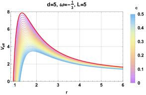
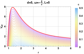
Figure 1: The variation of the effective potential as a function of the radial coordinate in different dimensions $d$, $c$ and two values of $\omega$, for $L=5$, $\mathcal{K}=1$ and $E=1$. In the all panels, the red curve corresponds to the Schwarzschild solutions.

It has been observed from Fig.1 that the potential for the Schwarzschild-Tangherlini black holes is relevant than the one surrounded by DE. Moreover, the potential increases with the dimension $d$. In this way, the unstable circular orbits become smaller. However, the $(-\frac{1}{3})$ and $(-\frac{2}{3})$-models exhibit the same maximum values showing a universal behavior with respect to such an effective potential. Another important remark is that the effective potential asymptote is constant within the large values of the radial coordinate $r$.

2.2 Shadow behavior

To deal with the photon orbit, we exploit two impact parameters $\eta$ and $\xi$, having a functional form in terms of the energy $E$, the angular momentum $L$, and the Carter constant $\mathcal{K}$ as follows

$$\xi=\frac{L}{E},\hskip 42.67912pt\eta=\frac{\mathcal{K}}{E^{2}}.$$ (2.44)

In this way, the effective potential and the function $\mathcal{R}(r)$ can be expressed as follows

$$V_{eff}=E^{2}(\frac{f_{\omega}(r)}{r^{2}}(\eta+\xi^{2})-1),\quad\mathcal{R}(r)=E^{2}(r^{4}-r^{2}f_{\omega}(r)(\eta+\xi^{2})).$$ (2.45)

Using (2.41) and (2.45), one can reveal that the impact parameters $\eta$ and $\xi$ should satisfy

$$\eta+\xi^{2}=\frac{5r_{0}^{2}}{3f_{\omega}(r_{0})+rf_{\omega}^{\prime}(r_{0})}.$$ (2.46)

To analyse the relevant data, the Tab.1 represents the variation of $\eta+\xi^{2}$ as a function of the dimension $d$, the DE state parameter $\omega$ and the field intensity $c$. It is worth noting that dimensional analysis reveals that $r_{0}$ has the dimension of the length while $\eta+\xi^{2}$ has the dimension of the length square, in $G=c=\hbar=1$ reduced units. To investigate the dimension effect on these physical quantities, we examine the results presented in Tab.1. From this table, we observe that for fixed values of $\omega$ and $c$, $\eta+\xi^{2}$ decreases by increasing the space-time dimension $d$ in contrary to the lower dimensions. Fixing the dimension $d$, $\eta+\xi^{2}$ increases by increasing $c$. Moreover, $\eta+\xi^{2}$ increases generally if one goes from the ($-\frac{1}{3}$)-model to the ($-\frac{2}{3}$)-model. Since the calculated values of $r_{0}$ and $\eta+\xi^{2}$ shown by dots in Tab.1 are complex having no physical meaning, they are not writing in the ($-\frac{2}{3}$)-model for ceratin values of the DE intensity $c$. Four dimensional behaviors, indeed, can be illustrated in Fig.2 for $\omega=-2/3$ with either $c=0.2$ or $c=0.3$.

	$c=0$		$\omega=-\frac{1}{3}$						$\omega=-\frac{2}{3}$
			$c=0.1$		$c=0.2$		$c=0.3$		$c=0.1$		$c=0.2$		$c=0.3$
	$r_{0}$	$\eta+\xi^{2}$	$r_{0}$	$\eta+\xi^{2}$	$r_{0}$	$\eta+\xi^{2}$	$r_{0}$	$\eta+\xi^{2}$	$r_{0}$	$\eta+\xi^{2}$	$r_{0}$	$\eta+\xi^{2}$	$r_{0}$	$\eta+\xi^{2}$
$d=4$	3	27	3.333	37.037	3.750	52.734	4.285	78.717	3.675	152.982	…	…	…	…
$d=5$	1.302	3.395	1.379	4.021	1.463	4.775	1.555	5.683	1.360	4.427	1.429	6.173	1.519	9.789
$d=6$	1.060	1.875	1.117	2.184	1.177	2.536	1.240	2.932	1.093	2.248	1.130	2.771	1.174	3.548
$d=7$	0.993	1.479	1.044	1.715	1.098	1.973	1.153	2.249	1.019	1.732	1.050	2.067	1.085	2.525
$d=8$	0.976	1.334	1.025	1.539	1.075	1.754	1.125	1.976	1.001	1.546	1.028	1.818	1.061	2.175
$d=9$	0.979	1.279	1.026	1.464	1.073	1.651	1.119	1.838	1.003	1.472	1.030	1.714	1.062	2.022
$d=10$	0.993	1.267	1.036	1.434	1.079	1.598	1.120	1.757	1.015	1.449	1.042	1.672	1.073	1.947
$d=11$	1.011	1.278	1.050	1.427	1.089	1.570	1.125	1.706	1.033	1.451	1.059	1.658	1.088	1.908

Table 1: $r_{0}$ and $\eta+\xi^{2}$ in higher dimensional space-time with DE.

It follows from this figure (dashed lines in left panel) that the function $f_{\omega}(r)$ becomes strictly negative avoiding the formation of black hole event horizon. It has been also observed that these non physical values are located outside the region of the values of positive $r_{0}$ in the diagram $M-c$ (black dots in right panel). Moreover, three different cases, i.e. double-horizons, single-horizon and no-horizon are depicted.

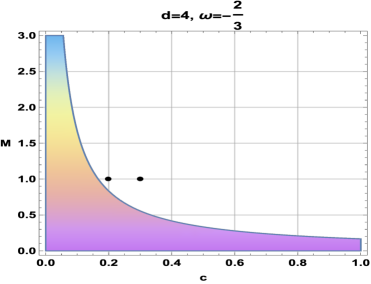
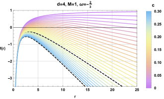
Figure 2: Left: Region Plot presents the allowed values of $r_{0}$ in the diagram $M-c$. Right: $f_{\omega}(r)$ in terms of $r$ with $m=1$, and different values of $c$. The two black points and two dashed black lines correspond to $c=0.2$ and $c=0.3$.

To properly visualize the shadow on the observer’s frame, one should use the celestial coordinates $\alpha$ and $\beta$ reported in [41]. Following to [5], the celestial coordinates $\alpha$ and $\beta$ have been taken as follows

$$\alpha=\lim_{r_{0}\to\infty}(\frac{r_{0}{P^{(\theta_{d-2})}}}{P^{(t)}}),\quad\beta_{i}=\lim_{r_{0}\to\infty}(\frac{r_{0}{P^{(\theta_{i})}}}{P^{(t)}}),\hskip 28.45274pti=1,\ldots,d-3,$$ (2.47)

where $r_{0}$ is the distance between the black hole and a far distant observer, and $\left[P^{(t)},P^{(\theta_{d-2})},P^{(\theta_{i})}\right]$ are the vi-tetrad component of momentum. Placing the observer on the equatorial hyperplane, these equations are reduced to

$$\alpha=-\xi,\hskip 28.45274pt\beta=\pm\sqrt{\eta}.$$ (2.48)

In this way, equation (2.46) can be rewritten as

$$\eta+\xi^{2}=\alpha^{2}+\beta^{2}.$$ (2.49)

It is worth noting that, in the absence of DE, we recover the Schwarzschild black hole result [6]. To inspect the DE effect on the shadow geometric circular shape, we plot, in Fig.3, the associated size behavior of $(-\frac{1}{3})$ and $(-\frac{2}{3})$-models in arbitrary dimension $d$ as a function of $c$. It follows from this figure that DE can be considered as a size shadow parameter. In particular, the associated size increases by increasing the field intensity $c$. Similar behaviors are observed with the DE state parameter. Switching from $(-\frac{1}{3})$-model to $(-\frac{2}{3})$-one, for a fixed $c$ value, this brings an increasing size circular geometry. Concretely, the present study reveals that DE leads to a violation of some bounds suggesting that the Schwarzschild solution is the biggest of all black holes for given masses [43, 42].
However, the increasing of the space-time dimension $d$ reduces the shadow circular size. For dimensions $d>11$, such a size remains constant allowing one to consider $d=11$ as a critical one for the shadow of the Schwarschild-Tanglerlini black hole with DE. It is worth noting that such a dimension, associated with a known theory called M-theory, has been approached in connection with dark sector from string axion fields [44]. It should be interesting to unveil certain links with M-theory in future works by focusing on such non-trivial stringy fields.

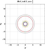
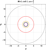
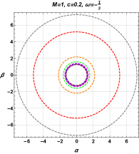
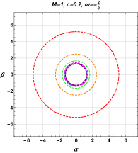
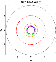
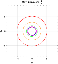
Figure 3: Black hole shadow in the celestial plane ($\alpha-\beta$ plane) for both models $(-\frac{1}{3})$ and $(-\frac{2}{3})$ within the dimension $d$ and the field intensity $c$. In the all panels, the red circle corresponds to the Schwarzschild black hole shadow without DE.

More inspections, on the photon behavior gravitating around the black hole at the distance of the photon sphere $r_{0}$ allow one to consider the ratio $\frac{R_{c}}{r_{0}}$ as a function of the dimension $d$. This is illustrated in Fig.4.

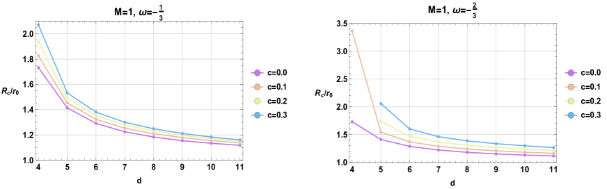
Figure 4: Variation of shadow radius $R_{c}$ over photon sphere radius $r_{0}$ as a function of dimension $d$, associated with $(-\frac{1}{3})$, $(-\frac{2}{3})$-models for different values of the intensity $c$.

It has been observed that for $d>6$ the radius of the photon sphere and the radius of the shadow circle are almost the same. Concretely, they are approximately confused for $(-\frac{1}{3})$ and $(-\frac{2}{3})$-models for different values $c$. However, $d\leq 6$, the radius $R_{c}$ is larger with respect to $r_{0}$.

2.3 Energy emission rate

It is known that, inside the black holes, quantum fluctuations create and annihilate a large number of particle pairs near the horizon. In this way, the positive energy particles escape through tunneling from the black hole, inside region where the Hawking radiation occurs. This process is known as the Hawking radiation causing the black hole to evaporate in a certain period of time. Here, we study the associated energy emission rate. In this case, for a far distant observer the high energy absorption cross section approaches to the black hole shadow. The absorption cross section of the black hole oscillates to a limiting constant value $\sigma_{lim}$ at very high energy. It turns out that the limiting constant value, being approximately equal to the area of photon sphere, can be expressed as

$$\frac{d^{2}E(\varpi)}{d\varpi dt}=\frac{2\pi^{2}\sigma_{lim}}{e^{\frac{\varpi}{T_{{out}}}}-1}\varpi^{(d-1)},$$ (2.50)

where $\varpi$ indicates the emission frequency [45]. It is noted that $T_{out}$ is the Hawking temperature for the Schwarzschild-Tangherlini with DE [46]. Such a temperature reads as

$$T_{{out}}=\frac{1}{4\pi}\left(\frac{d-3}{r}+c(d-1)\omega r^{-d(\omega+1)+\omega+2}\right).$$ (2.51)

According to [47, 48, 49], for a higher-dimensional space-time, $\sigma_{lim}$ can be given by

$$\sigma_{lim}\approx\frac{\pi^{(d-2)/2}R_{c}^{d-2}}{\Gamma(\frac{d}{2})}.$$ (2.52)

Using (2.52), we get the expression of the Schwarzschild-Tangherlini black hole energy emission rate in the presence of DE in higher-dimensional space-time as

$$\frac{d^{2}E(\varpi)}{d\varpi dt}=\frac{2\pi^{(d+2)/2}(\varpi R_{c})^{d-2}}{(e^{\frac{\varpi}{T_{{out}}}}-1)\Gamma(\frac{d}{2})}\varpi.$$ (2.53)

The energy emission rate is illustrated in Fig.5 as a function of $\varpi$ for different space-time dimensions and values of the DE intensity $c$.

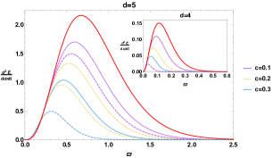
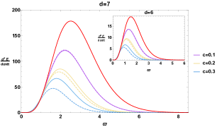
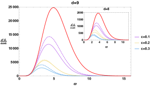
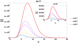
Figure 5: Energy emission rate for different dimensions $d$ and different values of DE the intensity $c$ where the red curve represents the case without DE. The straight lines represent the value $\omega=-1/3$ and the dashed ones are associated with $\omega=-2/3$.

It is observed from Fig.5 that, when DE is present, the energy emission rate is lower meaning that the black hole evaporation process is slow. Besides, we obtain an even slower radiation process by decreasing (increasing) the state parameter $\omega$ (the intensity $c$). However, increasing the dimension of the black hole implies a fast emission of particles. This shows that the evaporation of a higher dimensional black hole is fast compared to the one living in four dimensions. Furthermore, we can notice a special behavior for certain particular dimensions. For instance, the energy emission rate for the cases $d=6$ and $d=7$ for $\omega=-1/3$ and $\omega=-2/3$ models matches perfectly. This implies that some of the dimensions may show a resistance regarding the change of the state parameter. Taking into account of the studied models, the variation of the energy emission rate with respect to the space-time dimension reveals an intrigued behavior. Comparing the solid and dashed lines of each panel, one can notice that for $4\leqslant d\leqslant 7$ the emission associated with the $\omega=-\frac{1}{3}$ is more important than $\omega=-\frac{2}{3}$. However, for $8\leqslant d\leqslant 11$ the situation is inverted.

3 Deflection angle behavior of QBH in arbitrary dimensions

In this section, we study the behaviors of the deflection angle of quintessential Shwarzschild-Tanglerlini black holes by analysing the effect of various parameters including the space-time dimension $d$ and DE. It is recalled that such an angle can be computed from the relation

$$\Theta=-\iint_{S_{\infty}}{KdS},$$ (3.1)

where $K$ denotes the Gaussian curvature and where $dS$ is the surface of the associated optical metric [50]. It has been shown that this equation can be obtained by combining such a optical metric and the Gauss-Bonnet theorem. It is noted for a space denoted ($D_{R}$,$\chi$,$g$) where $D_{R}$ is the relevant region with a geometrical size $R$, $\chi$ is the associated Euler characteristic and $g$ is the corresponding Riemannian metric, the Gauss-Bonnet theorem stipulates

$$\iint_{D_{R}}{KdS}+\oint_{\partial D_{R}}{kdt}+\sum_{i}\eta_{i}=2\pi\chi(D_{R}).$$ (3.2)

Here, $k$ is the geodesic curvature given by $k=\bar{g}(\nabla_{\dot{\alpha}}\dot{\alpha},\ddot{\alpha})$ where $\ddot{\alpha}$ is the unit acceleration vector. For $R$ goes to $\infty$, the jump angles $\alpha_{s}$(source) and $\alpha_{O}$(observer) become $\alpha_{s}=\alpha_{o}=\frac{\pi}{2}$. The source and the observer interior angles are $\eta_{s}=\pi-\alpha_{s}$ and $\eta_{0}=\pi-\alpha_{0}$. For $\chi(D_{R})=1$ associated with a non-singular behavior, the Gauss-Bonnet theorem reduces to

$$\iint_{D_{R}}{KdS}+\oint_{\partial D_{R}}{kdt}+\eta=2\pi\chi(D_{R}),$$ (3.3)

where $\eta=\eta_{O}+\eta_{s}=\pi$. To obtain the relevant quantities including the Gaussian curvature, one should consider the equatorial hyperplane $\theta_{i}(i=1,\ldots,d-3)=\frac{\pi}{2}$. Using the notation $d\theta_{d-2}=d\phi^{2}$, the metric of the quintessential Schwarschild-Tanglerlini black holes given in (2.23) becomes

$$ds^{2}=f_{\omega}(r)dt^{2}+f_{\omega}(r)^{-1}dr^{2}+r^{2}d\phi^{2},$$ (3.4)

where now $ds^{2}$ denotes the optical metric. For null geodesics $ds^{2}=0$, one gets the optical metric tensor

$$dt^{2}=\frac{1}{f_{\omega}(r)^{2}}dr^{2}+\frac{r^{2}}{f_{\omega}(r)}d\phi^{2}.$$ (3.5)

In this way, the Gaussian curvature in the presence of DE can be obtained from the equation

$$K=\frac{{\mathbf{R}}}{2},$$ (3.6)

where ${\mathbf{R}}$ is the associated Ricci scalar. To get such quantities, the Christoffel symbols are needed. Indeed, the non-zero Christoffel symbols are given

$$\Gamma^{r}_{rr} = -\frac{f_{\omega}^{\prime}(r)}{f_{\omega}(r)},$$ (3.7)

$$\Gamma^{r}_{\phi\phi} = \frac{1}{2}r^{2}f_{\omega}^{\prime}(r)-rf_{\omega}(r),$$ (3.8)

$$\Gamma^{\phi}_{r\phi} = \frac{1}{r}-\frac{f_{\omega}^{\prime}(r)}{2f_{\omega}(r)},$$ (3.9)

where one has used $f_{\omega}^{\prime}(r)=\frac{\partial f_{\omega}(r)}{\partial r}$. It is noted that the Ricci scalar for the optical metric reads as

$${\mathbf{R}}=-\frac{1}{2}\Big{(}\frac{\partial f_{\omega}(r)}{\partial r}\Big{)}^{2}+f_{\omega}(r)\frac{\partial^{2}f_{\omega}(r)}{\partial r^{2}}.$$ (3.10)

The calculation shows that

$$\begin{split}f_{\omega}(r)\frac{\partial^{2}f_{\omega}(r)}{\partial r^{2}}=&-\bigg{(}1-\frac{\mu}{r^{d-3}}-\frac{c}{r^{\omega(d-1)+d-3}}\bigg{)}\bigg{(}\frac{\mu(d^{2}-5d+6)}{r^{d-1}}\\ &+c\Big{(}\frac{d^{2}(\omega^{2}+2\omega+1)}{r^{\omega(d-1)+d-1}}-\frac{d(2\omega^{2}+7\omega+5)+(\omega^{2}+5\omega+6)}{r^{\omega(d-1)+d-1}}\Big{)}\bigg{)},\end{split}$$ (3.11)

together with

$$\begin{split}\Big{(}\frac{\partial f_{\omega}(r)}{\partial r}\Big{)}^{2}=&\frac{(d-3)^{2}\mu^{2}}{r^{2d-4}}+\frac{c^{2}\big{(}d(\omega+1)-(\omega+3)\big{)}^{2}}{r^{2\omega(d-1)+2(d-2)}}\\ &+\frac{2\mu c\big{(}(d-3)(d(\omega+1)-(\omega+3))\big{)}}{r^{\omega(d-1)+2(d-2)}}.\end{split}$$ (3.12)

Using(3.6), we obtain

$$\begin{split}K=&-\mu\frac{(d^{2}-5d+6)}{2r^{d-1}}+\mu^{2}\frac{(d^{2}-4d+3)}{4r^{2(d-2)}}\\ &-c\Big{(}\frac{d^{2}(\omega^{2}+2\omega+1)-d(2\omega^{2}+7\omega+5)+(\omega^{2}+5\omega+6)}{2r^{\omega(d-1)+d-1}}\Big{)}\\ &+c\mu\Big{(}\frac{d^{2}(\omega^{2}+\omega+1)-d(2\omega^{2}+3\omega+4)+(\omega^{2}+2\omega+3)}{2r^{\omega(d-1)+2(d-2)}}\Big{)}\\ &+c^{2}\Big{(}\frac{d^{2}(\omega^{2}+2\omega+1)-d(2\omega^{2}+6\omega+4)+(\omega^{2}+4\omega+3)}{4r^{2\omega(d-1)+2(d-2)}}\Big{)}.\\ \end{split}$$ (3.13)

For simplicity reasons, we consider the Gaussian optical curvature up to the leading orders ($\mathcal{O}$($M^{2}$,$c^{2}$)) given by

$$\begin{split}K\approx&-\mu\frac{(d^{2}-5d+6)}{2r^{d-1}}+\\ &-c\Big{(}\frac{d^{2}(\omega^{2}+2\omega+1)-d(2\omega^{2}+7\omega+5)+(\omega^{2}+5\omega+6)}{2r^{\omega(d-1)+d-1}}\Big{)}\\ &+c\mu\Big{(}\frac{d^{2}(\omega^{2}+\omega+1)-d(2\omega^{2}+3\omega+4)+(\omega^{2}+2\omega+3)}{2r^{\omega(d-1)+2(d-2)}}\Big{)}.\\ \end{split}$$ (3.14)

To determine the deviation from the geodesic, it is useful to use the geodesic curvature

$$k(\gamma_{R})=|\nabla_{\gamma_{R}}\dot{\gamma_{R}}|,$$ (3.15)

$\gamma_{R}$ is a geodesic. Assuming that $\gamma_{R}=r(\phi)=R=const$, the radial part of the geodesic curvature reads as

$$(\nabla_{\gamma_{R}}\dot{\gamma_{R}})^{r}=\dot{\gamma_{R}}^{\phi}\partial_{\phi}\dot{\gamma_{R}}^{r}+\Gamma^{r}_{\phi\phi}(\dot{\gamma_{R}}^{\phi})^{2}.$$ (3.16)

According to [50], the second term provides

$$\oint_{\partial D_{R}}{kdt}=\pi+\Theta.$$ (3.17)

Using the linear approach of the light ray $(r=\frac{b}{\sin\phi})$ and equation (3.17), the deflection angle becomes

$$\Theta=-\int_{0}^{\pi}{\int_{\frac{b}{\sin\phi}}^{\infty}{KdS}},$$ (3.18)

where $b$ is called the impact parameter and $dS$ is given by

$$dS=\sqrt{det\bar{g}}\frac{dr}{f_{\omega}(r)}\approx rdr(1+\frac{3\mu}{2r^{d-3}}+\frac{3c}{r^{2\omega(d-1)+d-3}}).$$ (3.19)

Indeed, the deflection angle is approximated as follows

$$\Theta\approx-\int_{0}^{\pi}{\int_{\frac{b}{\sin\phi}}^{\infty}{Krdr}}.$$ (3.20)

Using the result $\int_{0}^{\pi}{\int_{\frac{b}{\sin\phi}}^{\infty}{r^{-n}}}=\frac{\sqrt{\pi}nb^{1-n}\Gamma\left(\frac{n}{2}\right)}{(n-1)\Gamma\left(\frac{n+1}{2}\right)}$ and the expression of $K$ given in (3.14), we get

$$\begin{split}\Theta\approx&\frac{c\sqrt{\pi}(\omega(d-1)+d-2)\Gamma\left(\frac{1}{2}(\omega(d-1)+d-2)\right)b^{\omega(1-d)+3-d}}{2\Gamma\left(\frac{1}{2}(d-1)(\omega+1)\right)}\\ &-\Bigg{(}\frac{c\mu\sqrt{\pi}(d-1)\left(\omega^{2}(d-1)+\omega(d-2)+d-3\right)}{2(\omega(d-1)+2d-6)}\\ &\times\frac{\Gamma\left(\frac{1}{2}(\omega(d-1)+2d-5)\right)b^{-d(\omega+2)+\omega+6}}{\Gamma\left(\frac{\omega}{2}(d-1)+d-2\right)}\Bigg{)}+\frac{\mu\sqrt{\pi}\Gamma\left(\frac{d}{2}\right)b^{3-d}}{\Gamma\left(\frac{d-1}{2}\right)}+\mathcal{O}(M^{2},c^{2}).\end{split}$$ (3.21)

Applying a power series expansion, we obtain the deflection angle of the quintessential Schwarschild-Tanglerlini black holes

$$\Theta\approx\frac{\sqrt{\pi}\mu b^{3-d}\Gamma\left(\frac{d}{2}\right)}{\Gamma\left(\frac{d-1}{2}\right)}+\frac{c\omega(d-1)\sqrt{\pi}}{4}(A-B)+\mathcal{O}(M^{2},c^{2},\omega^{2}),$$ (3.22)

where the involved terms $A$ and $B$ take the following form

$$A = \frac{\mu\Gamma\left(\frac{1}{2}(2d-5)\right)b^{6-2d}}{2\Gamma(d-2)}\Bigg{(}(d-1)\Big{(}2\log(b)+\psi^{(0)}(d-2)\Big{)}$$ (3.23)

$$+ (1-d)\psi^{(0)}\left(\frac{2d-5}{2}\right)-\frac{(\omega+2)}{\omega}\Bigg{)},$$

$$B = \frac{\Gamma\left(\frac{d-2}{2}\right)b^{3-d}}{\Gamma\left(\frac{d-1}{2}\right)}\Bigg{(}2(d-2)\Big{(}\log(b)-\frac{1}{\omega(d-1)}-\frac{1}{(d-2)}\Big{)}$$

$$+ \Bigg{(}\psi^{(0)}\left(\frac{d-1}{2}\right)-\psi^{(0)}\left(\frac{d-2}{2}\right)\Bigg{)}\Bigg{)}.$$

Here, $\psi$ is the polygamma function defined as follows

$$\psi^{n}(z)={\frac{d^{n}}{dz^{n}}}\psi(z)={\frac{d^{{n+1}}}{dz^{{n+1}}}}\ln\Gamma(z),\quad\psi^{(0)}(z)=\psi(z)=\frac{\Gamma^{\prime}(z)}{\Gamma(z)}.$$ (3.24)

Having computed the deflection angle, we move to analyse and discuss the associated behavior. In particular, we consider the effect of the impact parameter $b$, DE, and the dimension on such quantity. In Fig.6, we represent, indeed, the variation of the deflection angle $\Theta$ as a function of the parameter $b$ in different dimensions $d$ with DE. It follows from such a figure, based on the top panels one, that $\Theta$ decreases by increasing the impact parameter $b$ and it increases by increasing the field intensity $c$. In the two bottom panels, we observe that the deflection angle $\Theta$ decreases gradually when the dimension of the space-time $d$ increases.

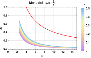
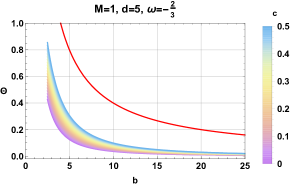
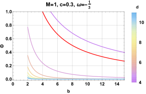
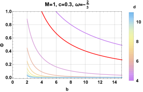
Figure 6: Variation of the deflection angle as a function of the parameter $b$ in different dimension $d$, $c$ and for two values of $\omega$. In the all panels, the red curve corresponds to deflection of Schwarzschild black hole without DE.

To better visualize such a behavior, we plot in Fig.7 the variation of $\Theta$ in terms of the space-time dimensions $d$ for fixed values of the impact parameter $b$.

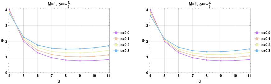
Figure 7: Variation of $\Theta$ as function of the space-time dimensions $d$ for fixed parameter $b=1$.

It follows from this figure that the effect of DE on $\Theta$ becomes relevant from $d=5$. Such an angle, being relevant in $d=4$, decreases with space-time dimension $d$. However, for higher dimensions it is almost constant. Its value increases with the DE intensity field $c$. This visible behavior seems to have possible connections with ideas corresponding to DE as the extra dimension evidence predicted by M-theory and superstring models.

4 Optical behaviors from the charge effect

In this section, we unveil more behaviors by introducing the charge effect. To start, the associated metric function $f_{\omega}(r)$ reads as

$$f_{\omega}(r)=1-\frac{\mu}{r^{d-3}}+\frac{Q^{2}}{r^{2(d-3)}}-\frac{c}{r^{\omega(d-1)+d-3}},$$ (4.1)

where $Q$ is the charge of the black hole. It has been observed that for $d>4$, the solution of the associated equation generates two radius photon spheres $r_{0}$(max) and $r_{0}$(min). This gives two radius of the shadow circles. However, to deal with the shadow behaviors, one should use the maximum one, as shown in Fig.8. It has been remarked that the charge increases the shadow size for fixed values of $c$ and $\omega$. A close inspection shows that non trivial behaviors arise for the charged case compared to the results of the non-charged black hole shadows presented in Fig.3. In $d=4$, we observe that for constant values of the charge and for $d>4$, $c=0$ or $c>0.2$, the shadow size decreases. However, for $d>4$ and $0<c<0.2$ such behaviors depend strongly on the charge where the shadow size increases. This is probably due to the competition between the positive charge therm and the negative DE term in the blacking function in Eq.(4.1). We expect also that such behaviors could be related to extra dimensions supporting the discussion of DE from many aspects.

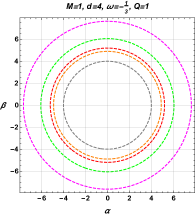
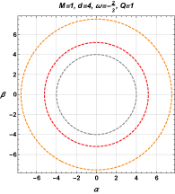
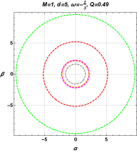
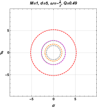
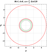
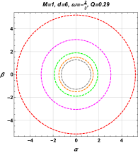
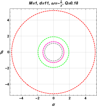
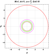
Figure 8: Shadow of charged black hole with DE $(-\frac{1}{3})$-model and $(-\frac{2}{3})$-model in different dimension $d$ as a function of $c$. In the all panels, the red circle corresponds to the Schwarzschild black hole shadow without DE and charge $(d=4,\ c=0,\ Q=0)$.

To go deeply in such an analysis related to the charge black hole effect, we use the same precedent procedure to evaluate the deflection angle behaviors. Using (3.5) and the metric function $f_{\omega}(r)$ of the charged black solution, we get the optical metric in the higher dimensional space-time. Similar calculations show that the Gaussian curvature of the optical charged black hole up to leading orders ($\mathcal{O}$($M^{2}$,$c^{2}$)) can be given by

$$\begin{split}\mathcal{K}\approx&\left(2d^{2}-11d+15\right)Q^{2}r^{4-2d}-\frac{\mu\left(d^{2}-5d+6\right)}{2}\left(3Q^{2}r^{7-3d}+r^{1-d}\right)\\ &-\frac{1}{2r^{\omega(d-1)}}\Bigg{(}\Big{(}\left(d^{2}-2d+1\right)\omega^{2}+\left(2d^{2}-7d+5\right)\omega+\left(d^{2}-5d+6\right)\Big{)}r^{1-d}\\ &+Q^{2}\Big{(}\left(d^{2}-2d+1\right)\omega^{2}+(d-1)\omega+\left(3d^{2}-15d+18\right)\Big{)}r^{7-3d}\\ &-\mu\left(d^{2}-2d+1\right)\omega^{2}+\left(d^{2}-3d+2\right)\omega+\left(d^{2}-4d+3\right)r^{4-2d}\Bigg{)}c.\end{split}$$ (4.2)

It is remarked that this result recovers the Gaussian curvature of optical four dimensional charged black hole presented in [51] and the higher dimensional case investigated in the previous section. Exploiting a power series expansion, we obtain the deflection angle

$$\begin{split}\delta\approx&\Theta-\frac{Q^{2}}{12}\sqrt{\pi}b^{6-3d}\Bigg{(}\frac{12b^{d}\Gamma\left(\frac{2d-3}{2}\right)}{\Gamma(d-2)}+\frac{b^{3}}{\Gamma\left(\frac{3d-7}{2}\right)}\Bigg{(}c\Big{(}D+E+F\Big{)}+6(2-d)\mu\Bigg{)}\Bigg{)}\\ &+\mathcal{O}(M^{2},c^{2},\omega^{2}),\end{split}$$ (4.3)

where one has

$$D = d^{2}\left(6\epsilon\log(b)-3\epsilon\psi^{(0)}\left(\frac{3d}{2}-4\right)+3\epsilon\psi^{(0)}\left(\frac{1}{2}(3d-7)\right)\right),$$ (4.4)

$$E = d\left(-18\epsilon\log(b)+9\epsilon\psi^{(0)}\left(\frac{3d}{2}-4\right)-9\epsilon\psi^{(0)}\left(\frac{1}{2}(3d-7)\right)+2\epsilon-6\right),$$ (4.5)

$$F = \left(12\epsilon\log(b)-6\epsilon\psi^{(0)}\left(\frac{3d}{2}-4\right)+6\epsilon\psi^{(0)}\left(\frac{1}{2}(3d-7)\right)-2\epsilon+12\right),$$ (4.6)

and where $\Theta$ is nothing but the deflection angle of the non-charged QBH (3.22). For $d=4$, we recover the same result for the charged black hole [52, 51].

In Fig.9, we illustrate the charge effect on the deflection angle.

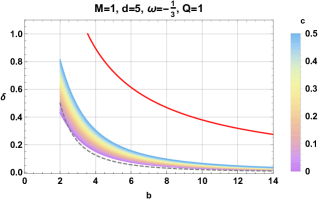
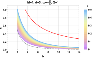
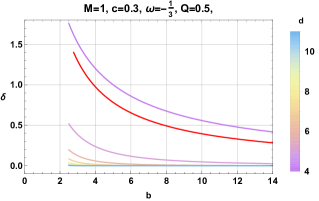
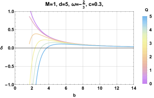
Figure 9: Variation of $\delta$ as a function of dimensions $d$ for different values of $c$ and for fixed parameter $b$ and $Q$. In the all panels, the gray dashed line curve corresponds to the Schwarzschild black hole shadow without DE and charge in $d=5$.

For a fixed charge value, the variation of $\delta$ in terms of the impact parameter and the field intensity $c$ remain the same as the neutral case. Thus means that $\delta$ decreases gradually within $b$. However, we can easily notice that the growth of $c$ increases $\delta$. The left right panel indicates that when the charge $Q$ increases the deflection angle $\delta$ decreases.

5 Shadow behavior in the presence of the plasma

The present approach can be adaptable to a broad variety of backgrounds. It has been remarked that the previous space-time can be modified by a non-trivial background associated with a non-magnetized cold plasma [53]. According to [54, 55, 56], the frequency $\omega_{p}$ of the electron plasma can be written, using a radial power law, as follows

$$\omega_{p}^{2}(r)=\frac{k}{r^{h}},\qquad h\geq 0.$$ (5.1)

Using the plasma frequency $\omega_{p}$ and the photon frequency $\omega_{0}$, the refraction index of such a background reads as

$$n^{2}(r,\omega_{0})=1-\frac{\omega^{2}_{p}(r)}{\omega^{2}_{0}}.$$ (5.2)

In this situation, certain vacuum equations including the equations of motion for photon around QBH can be modified. In particular, the relevant ones become

$$\frac{dt}{d\tau} = \frac{n^{2}(r,\omega_{0})E}{f_{\omega}(r)},$$ (5.3)

$$\mathcal{R}(r) = n^{2}(r,\omega_{0})E^{2}r^{4}-r^{2}f_{\omega}(r)(\mathcal{K}+L^{2}).$$ (5.4)

Using Eq.(2.41), the impact parameters $\eta$ and $\xi$ can be generalized to

$$\eta+\xi^{2}=\frac{5n^{2}(r_{0},\omega_{0})r_{0}^{2}+2n(r_{0},\omega_{0})n^{\prime}(r_{0},\omega_{0})r^{3}_{0}}{3f_{\omega}(r_{0})+rf_{\omega}^{\prime}(r_{0})},$$ (5.5)

where the prime indicates the derivative with respect to $r$. Redefining the celestial coordinates (2.48) associated with the equatorial hypeplan as follows

$$\alpha=-\frac{\xi}{n(r_{0},\omega_{0})},\hskip 28.45274pt\beta=\pm\frac{\sqrt{\eta}}{n(r_{0},\omega_{0})},$$ (5.6)

the equation (5.5) can be reexpressed as

$$\alpha^{2}+\beta^{2}=\frac{\xi^{2}+\eta}{n^{2}(r_{0},\omega_{0})}=\frac{5n^{2}(r_{0},\omega_{0})r_{0}^{2}+2n(r_{0},\omega_{0})n^{\prime}(r_{0},\omega_{0})r^{3}_{0}}{n^{2}(r_{0},\omega_{0})\big{(}3f_{\omega}(r_{0})+rf_{\omega}^{\prime}(r_{0})\big{)}}.$$ (5.7)

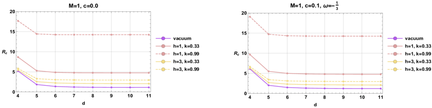
Figure 10: Variation of shadow radius $R_{c}$ as a function dimension $d$, without DE and for the $(-\frac{1}{3})$-model for different values of the intensity $h$ and $k$.

Fig.10 shows the variation of the shadow radius in the presence of plasma as a function of the space-time dimension $d$ with and without DE. Turning off DE, we have observed that the plasma presence increases the shadow radius $R_{c}$. For $h=1$, we have remarked also that $R_{c}$ increases when $k$ increases. The implementation of DE, however, has revealed that the shadow radius increases only for $4\leq d\leq 6$. The higher dimensional cases seem to have approximatively the ordinary behaviors. We expect that other optical properties could be also approached in such plasma backgrounds by performing similar calculations.

6 Conclusions and open questions

Motivated by M-theory/superstring inspired models, we have investigated certain behaviors of the deflection angle and shadow circular shapes of higher dimensional QBH associated with $\omega=-\frac{1}{3}$ and $\omega=-\frac{2}{3}$ models. In particular, we have derived the complete geodesic structure of photons around such black holes using the Hamilton-Jacobi equation and Carter’s constant separable method. Linking the celestial coordinate to the geodesic equations and plotting the black hole shadow shape within the field intensity $c$ and the dimension of the space-time $d$, we have found that $d$ decreases the shadow size. However, DE increases such a geometrical size. Moreover, we have computed the energy emission rate of the black hole by assuming that the area of the photon sphere is equal to the high-energy absorption cross-section. Then, we have analyzed the effect of the DE field intensity $c$ and the space-time dimension $d$ on such a quantity. In the second part of the present work, we have approached the weak deflection angle of light of such higher dimensional QBH. Precisely, this has been done by determining the corresponding optical Gaussian curvature. Using the Gauss-Bonnet theorem associated with the optical metric, we have calculated the leading terms of the deflection angle in the weak-limit approximation. Besides, we have discussed the impact of DE and the space-time dimension $d$ on such a optical quantity. In the last part, we have analyzed the effect of the charge $Q$ on all the above-computed quantities, which not only provides non-trivial behaviors but also recovers the ordinary ones.

In a arbitrary dimensional space-time, it has been shown that the quintessence field increases the size of shadows. According to four-dimensional results reported in [57], we could expect that such a field imposes an impact on the size of the image of black hole and the distances between the observer and the horizon of the event through the state parameter. In this way, the positions of the photon spheres of the image could be modified. In future EHT experiments, the observations of black hole shadow images could provide insights and certain signatures associated with the quintessential dark energy physical models.
In coming works, we attempt to study the impact of the equivalency principle on the black hole in the presence of quintessence fields by incorporating the spinning parameter explored in [58]. We anticipate that the principle of equivalence could remain in the case of the non-rotating black hole in the presence of quintessence fields. However, the rotating parameter may bring non-trivial results, which will be explored elsewhere.

This work comes up with many questions. The natural one is to make contact with evidence of DE from extra dimensions. We hope to address such a question in future by considering M-theory analysis associated with the axionic universe. Connections with Dark Matter could be also possible [59]. Moreover, based on the event telescope and black hole investigations, one could say that one involves new and powerful tools to approach the so called new physics beyond standard model.

Appendix A Einstein equations in $d$-dimensional space-time

In this appendix, we collect some calculations associated with the higher dimensional quantities used trough this work.

Christoffel symbols

$$\begin{split}&\Gamma^{t}_{t\,\,r}\;=\;\frac{\nu^{\prime}}{2},\\ &\Gamma^{r}_{t\,\,t}\;=\;\frac{\nu^{\prime}e^{\nu-\lambda}}{2},\\ &\Gamma^{r}_{\theta_{i}\,\,\theta_{i}}\;=\;-re^{-\lambda}\prod_{j=1}^{i-1}\sin^{2}{\theta_{j}},\hskip 28.45274pti=1,\ldots,d-2,\\ &\Gamma^{\theta_{i}}_{r\,\,\theta_{i}}\;=\;\frac{1}{r},\hskip 28.45274pti=1,\ldots,d-2,\\ &\Gamma^{\theta_{k}}_{\theta_{i}\,\,\theta_{i}}\;=\;-\cos{\theta_{k}}\sin{\theta_{k}}\prod_{j=k+1}^{i-1}\sin^{2}{\theta_{j}},\hskip 28.45274ptk=1,\ldots,d-3,\hskip 14.22636pti=k+1,\ldots,d-2,\\ &\Gamma^{\theta_{k}}_{\theta_{i}\,\,\theta_{k}}\;=\;\cot\theta_{i},\hskip 28.45274ptk=2,\ldots,d-2,\hskip 14.22636pti=1,\ldots,k-1.\end{split}$$ (A.1)

where $\nu^{\prime}=\frac{\partial\nu}{\partial r}$ and $\lambda^{\prime}=\frac{\partial\lambda}{\partial r}$.

Riemann tensor

$$\begin{split}&\mathrm{R}^{t}_{r\,\,r\,t}\;=\;\frac{-\lambda^{\prime}\nu^{\prime}+\nu^{\prime 2}+2\nu^{\prime\prime}}{4},\\ &\mathrm{R}^{t}_{\theta_{i}\,\,\theta_{i}\,t}\;=\;\frac{r\nu^{\prime}e^{-\lambda}}{2}\prod_{j=1}^{i-1}\sin^{2}\theta_{j},\hskip 28.45274pti=1,\ldots,d-2,\\ &\mathrm{R}^{r}_{\theta_{i}\,\,\theta_{i}\,r}\;=\;-\frac{r\lambda^{\prime}e^{-\lambda}}{2}\prod_{j=1}^{i-1}\sin^{2}\theta_{j},\hskip 28.45274pti=1,\ldots,d-2,\\ &\mathrm{R}^{r}_{t\,\,r\,t}\;=\;\frac{e^{\nu-\lambda}(-\lambda^{\prime}\nu^{\prime}+\nu^{\prime 2}+2\nu^{\prime\prime})}{4},\\ &\mathrm{R}^{\theta_{i}}_{t\,\theta_{i}\,t}\;=\;\frac{e^{\nu-\lambda}\nu^{\prime}}{2r},\hskip 28.45274pti=1,\ldots,d-2,\\ &\mathrm{R}^{\theta_{i}}_{r\,\theta_{i}\,r}\;=\;\frac{\lambda^{\prime}}{2r},\hskip 28.45274pti=1,\ldots(d-2),\\ &\mathrm{R}^{\theta_{i}}_{\theta_{k}\,\theta_{k}\,\theta_{i}}\;=\;(e^{-\lambda}-1)\prod_{j=1}^{k-1}\sin^{2}\theta_{j},\hskip 28.45274pti=1,\ldots,d-3,\hskip 14.22636ptk=i+1,\dots,d-2,\\ &\mathrm{R}^{\theta_{i}}_{\theta_{k}\,\theta_{k}\,\theta_{i}}\;=\;(1-e^{-\lambda})\prod_{j=1}^{k-1}\sin^{2}\theta_{j},\hskip 28.45274pti=2,\ldots,d-2,\hskip 14.22636ptk=1,\ldots,i-1.\end{split}$$ (A.2)

Ricci tensor

$$\begin{split}&{R_{t\,\,t}}\;=\;\frac{e^{\nu-\lambda}(\nu^{\prime}((2d-4)-r\lambda^{\prime})+r\nu^{\prime 2}+2r\nu^{\prime\prime})}{4r},\\ &{R_{r\,\,r}}\;=\;\frac{\lambda^{\prime}((2d-4)+r\nu^{\prime})-r(\nu^{\prime 2}+2\nu^{\prime\prime})}{4r},\\ &{R_{\theta_{i}\,\theta_{i}\,}}\;=\;\frac{e^{-\lambda}}{2}((2d-6)(e^{-\lambda}-1)+r(\lambda^{\prime}-\nu^{\prime}))\prod_{j=1}^{i-1}\sin^{2}\theta_{j},\hskip 28.45274pti=1,\ldots,d-2.\end{split}$$ (A.3)

Scalar curvature

$$R\;=\;\sum^{d-2}_{i=1}\frac{(r(\nu^{\prime}-\lambda^{\prime})+(2d-6)(1-e^{\lambda}))e^{\lambda}}{2r^{2}}\,+\,\frac{e^{-\lambda}\left((d-2)\nu^{\prime}-\lambda^{\prime}\left(d+r\nu^{\prime}-2\right)+2r\nu^{\prime\prime}+r\left(\nu^{\prime}\right)^{2}\right)}{2r}.$$ (A.4)

Einstein tensor

$$\begin{split}&{G_{t\,\,t}}\;=\;\frac{(d-2)e^{\nu-\lambda}\left((d-3)\left(e^{\lambda}-1\right)+r\lambda^{\prime}\right)}{2r^{2}},\\ &G_{r\,\,r}\;=\;\frac{(d-2)\left((d-3)\left(1-e^{\lambda}\right)+r\nu^{\prime}\right)}{2r^{2}},\\ &{G_{\theta_{i}\,\theta_{i}\,}}\;=\;\frac{1}{4}e^{-\lambda}\left(2(d-3)r\left(\nu^{\prime}-\lambda^{\prime}\right)+2(d-4)(d-3)-r^{2}\lambda^{\prime}\nu^{\prime}+2r^{2}\nu^{\prime\prime}+r^{2}\left(\nu^{\prime}\right)^{2}\right)\\ &\hskip 44.10185pt-\frac{1}{2}(d-3)(d-4)\prod_{j=1}^{i-1}\sin^{2}\theta_{j},\hskip 28.45274pti=1,\ldots,d-2.\end{split}$$ (A.5)

Einstein equation

In the reduced units, we give

$$\begin{split}&2T_{t}^{\;t}\;=\frac{(d-2)e^{-\lambda}\left((d-3)\left(e^{\lambda}-1\right)+r\lambda^{\prime}\right)}{2r^{2}},\\ &2T_{r}^{\;r}\;=\;\frac{(d-2)e^{-\lambda}\left((d-3)\left(e^{\lambda}-1\right)-r\nu^{\prime}\right)}{2r^{2}},\\ &2T_{\theta_{i}}^{\;\theta_{i}}\;=\;-\frac{e^{-\lambda}\left(2(d-3)r\left(\nu^{\prime}-\lambda^{\prime}\right)+2(d-4)(d-3)-r^{2}\lambda^{\prime}\nu^{\prime}+2r^{2}\nu^{\prime\prime}+r^{2}\left(\nu^{\prime}\right)^{2}\right)}{4r^{2}}\\ &\hskip 44.10185pt+\frac{(d-3)(d-4)}{2r^{2}}\hskip 28.45274pti=1,\ldots,d-2.\end{split}$$ (A.6)

References

- [1] K. Akiyama, et al., Event Horizon Telescope Collaboration Astrophys. J., 875 (1) (2019), p. L1.
- [2] K. Akiyama, et al., Event Horizon Telescope Collaboration Astrophys. J., 875 (1) (2019), p. L4.
- [3] C. Goddi et al., BlackHoleCam: Fundamental physics of the galactic center, Int.J.Mod.Phys.D 26 (2016) 1730001, arXiv:1606.08879.
- [4] A. De Vries, The apparent shape of a rotating charged black hole, closed photon orbits and the bifurcation set A4, Classical and Quantum Gravity 17 (1) (2000)123.
- [5] C. Subrahmanyan, The mathematical theory of black holes, Oxford University Press, 1992.
- [6] B. P. Singh, S. G. Ghosh, Shadow of Schwarzschild–Tangherlini black holes, Annals of Physics 395 (2018)127, arXiv:1707.07125.
- [7] A. Strominger, C. Vafa, Microscopic Origin of the Bekenstein-Hawking Entropy, Phys. Lett. B379 (1996)99.
- [8] R. Emparan, H. S. Reall, Black Holes in Higher Dimensions, Living Rev. Relativ. 11 (2008) 6.
- [9] V. Cardoso, E. Franzin and P. Pani, Is the gravitational-wave ringdown a probe of the event horizon?, Phys. Rev. Lett.116 no.17 (2016) 171101, arXiv:1602.07309.
- [10] H. Yu, B. M. Gu, F. P. Huang, Y. Q. Wang, X. H. Meng and Y. X. Liu, Probing extra dimension through gravitational wave observations of compact binaries and their electromagnetic counterparts, JCAP 02 (2017) 039, arXiv:1607.03388.
- [11] L. Visinelli, N. Bolis and S. Vagnozzi, Brane-world extra dimensions in light of GW170817, Phys. Rev. D97 no.6(2018) 064039, arXiv:1711.06628.
- [12] O. K. Kwon, S. Lee and D. D. Tolla, Gravitational Waves as a Probe of the Extra Dimension, Phys. Rev. D 100 (2019) 084050, arXiv:1906.11652.
- [13] S. Vagnozzi and L. Visinelli, Hunting for extra dimensions in the shadow of M87*, Phys. Rev. D100no.2 (2019) 024020, arXiv:1905.12421.
- [14] V. Perlick, Gravitational lensing from a spacetime perspective, Living Rev. Rel. 7, (2004)9.
- [15] V. Perlick, O. Y. Tsupko, G. S. Bisnovatyi-Kogan, Black hole shadow in an expanding universe with a cosmological constant, Phys. Rev. D 97, no.10, (2018)104062, arXiv:1804.04898.
- [16] S. D. Epps, M. J. Hudson, The Weak Lensing Masses of Filaments between Luminous Red Galaxies, Mon. Not. Roy. Astron. Soc. 468, no.3,(2017) 2605, arXiv:1702.08485.
- [17] M. Bartelmann, M. Maturi, Weak gravitational lensing, arXiv:1612.06535.
- [18] C. Bambi, K. Freese, S. Vagnozzi, L. Visinelli, Testing the rotational nature of the supermassive object M87* from the circularity and size of its first image, Phys. Rev. D100, no.4, (2019)044057, arXiv:1904.12983.
- [19] A. Allahyari, M. Khodadi, S. Vagnozzi, D. F. Mota, Magnetically charged black holes from non-linear electrodynamics and the Event Horizon Telescope, JCAP 02(2020) 003, arXiv:1912.08231.
- [20] P. V. Cunha, C. A. R. Herdeiro, B. Kleihaus, J. Kunz, E. Radu, Shadows of Einstein–dilaton–Gauss–Bonnet black holes, Phys. Lett. B768(2017)373, arXiv:1701.00079.
- [21] R. Shaikh, P. Kocherlakota, R. Narayan, P. S. Joshi, Shadows of spherically symmetric black holes and naked singularities, Mon. Not. Roy. Astron. Soc. 482, no.1, (2019)52, arXiv: 1802.08060.
- [22] T. Zhu, Q. Wu, M. Jamil, K. Jusufi, Shadows and deflection angle of charged and slowly rotating black holes in Einstein-Æther theory, Phys. Rev. D100(2019) 044055, arXiv:1906.05673.
- [23] A. Belhaj, A. El Balali, W. El Hadri, M. A. Essebani, M. B. Sedra, A. Segui, Kerr-AdS Black Hole Behaviors from Dark Energy, Int. Jour. of Mod. Phys. D29 (09) (2020) 2050069.
- [24] P.W. Higgs, Broken symmetries, massless particles and gauge elds, Phys. Lett.12 (1964) 132.
- [25] D. Matravers, Steven Weinberg: Cosmology, Gen Relativ Gravit 41 (2009)1455.
- [26] P.J.E. Peebles, B. Ratra, The cosmological constant and dark energy, Rev.Mod.Phys.75(2003)559.
- [27] N. Jarosik et al. [WMAP], Seven-Year Wilkinson Microwave Anisotropy Probe (WMAP) Observations: Sky Maps, Systematic Errors, and Basic Results, Astrophys. J. Suppl. 192 (2011) 14, arXiv:1001.4744.
- [28] P. R. Kafle, S. Sharma, G. F. Lewis, J. Bland-Hawthorn, On the Shoulders of Giants: Properties of the Stellar Halo and the Milky Way Mass Distribution, Astrophys. J. 794 (2014) 59, arXiv:1408.1787.
- [29] A. G. Riess et al. [Supernova Search Team], Type Ia supernova discoveries at z ¿ 1 from the Hubble Space Telescope: Evidence for past deceleration and constraints on dark energy evolution, Astrophys. J.607 (2004) 665, astro-ph/0402512.
- [30] Planck Collaboration, P.A.R. Ade, et al., Planck intermediate results - XVI. Profile likelihoods for cosmological parameters, Astronomy and Astrophysics 571, (2014)A16.
- [31] Planck Collaboration, P.A.R. Ade, et al., Astronomy and Astrophysics 566, (2014)A54.
- [32] Z. Stuchlik, The motion of test particles in black-hole backgrounds with non-zero cosmological constant, Bulletin of the Astronomical Institutes of Czechoslovakia 34 129 (1983) 11.
- [33] V. Perlick, O. Yu. Tsupko, G. S. Bisnovatyi-Kogan, Black hole shadow in an expanding universe with a cosmological constant. Phys. Rev. D97(10)(2018)104062.
- [34] J.P. Uzan, G.F.R. Ellis, J. Larena, A two-mass expanding exact space-time solution, General Relativity and Gravitation 43 (2011)191.
- [35] V. V. Kiselev, Quintessence and black holes, Class. Quant. Grav. 20 (2003) 1187, gr-qc/0210040.
- [36] A. Belhaj, A. El Balali, W. El Hadri, Y. Hassouni, E. Torrente-Lujan, Phase Transitions of Quintessential AdS Black Holes in M-theory/Superstring Inspired Models, arXiv:2004.10647.
- [37] F.R. Tangherlini, Schwarzschild field in n dimensions and the dimensionality of space problem, Nuovo Cim. 27 (1963) 636.
- [38] S. Chen, B. Wang, R. Su, Hawking radiation in a d-dimensional static spherically symmetric black hole surrounded by quintessence, Phys. Rev. D 77 (2008) 124011.
- [39] B. Carter, Global structure of the Kerr family of gravitational fields, Physical Review 174(5)(1968) 1559
- [40] B. Carter, Global Structure of the Kerr Family of Gravitational Fields, Phys. Rev. 174 (1968)1559.
- [41] S. Vazquez, E. P. Esteban, Strong field gravitational lensing by a Kerr black hole, Nuovo Cim.B119(2004)489.
- [42] H. Lu, H. D. Lyu, Schwarzschild black holes have the largest size, Phys. Rev. D101, no.4, (2020) 044059, arXiv:1911.02019.
- [43] S. Hod, Upper bound on the radii of black-hole photonspheres, Phys. Lett. B727 (2013)345, arXiv:1701.06587.
- [44] B. S. Acharya, S. A. R. Ellis, G. L. Kane, B. D. Nelson, M. Perry, Categorisation and Detection of Dark Matter Candidates from String/M-theory Hidden Sectors, JHEP09(2018)130, arXiv:1707.04530.
- [45] S. W. Wei and Y. X. Liu, Observing the shadow of Einstein-Maxwell-Dilaton-Axion black hole, JCAP 11 (2013)063, arXiv:1311.4251.
- [46] A. Belhaj, A. El Balali, W. El Hadri, H. El Moumni, M. B Sedra, Dark energy effects on charged and rotating black holes, Eur. Phys. J. Plus 134(2019) 422.
- [47] L. Peng-Cheng, G. Minyong, B. Chen, Shadow of a Spinning Black Hole in an Expanding Universe, Phys. Rev. D101 (2020)084041, arXiv:2001.0423.
- [48] W. Shao-Wen, L. Yu-Xiao, Observing the shadow of Einstein-Maxwell-Dilaton-Axion black hole, CAP 11 (2013) 063, arXiv:1311.4251.
- [49] Y. Décanini, A. Folacci, B. Raffaelli, Fine structure of high-energy absorption cross sections for black holes, Class. Quantum Grav. 28(2011) 175021.
- [50] G. Gibbons and M. Werner, Applications of the Gauss-Bonnet theorem to gravitational lensing, Class. Quant. Grav. 25 (2008) 235009, arXiv:0807.0854.
- [51] W. Javed, J. Abbas, A. Övgün, Effect of the quintessential dark energy on weak deflection angle by Kerr–Newmann Black hole, Annals of Physics (2020)168183.
- [52] W. Javed, A. Hamza, A. Övgün, Effect of Non-linear Electrodynamics on Weak field deflection angle by Black Hole, Phys. Rev. D101 (2020) 103521, arXiv:2005.09464.
- [53] F. Atamurotov and B. Ahmedov, Optical properties of black hole in the presence of plasma: shadow, Phys. Rev. D 92 (2015) 084005, arXiv:1507.08131.
- [54] R. Adam, Frequency-dependent effects of gravitational lensing within plasma, Monthly Notices of the Royal Astronomical Society, (2015) 4536, arXiv:1505.06790.
- [55] J.L. Synge, Relativity: The General Theory, (North- Holland, Amsterdam, 1960).
- [56] A. Abdujabbarov, B. Toshmatov, Z. Stuchlík, B. Ahmedov, Shadow of the rotating black hole with quintessential energy in the presence of plasma, Int. J. Mod. Phys. D26, no.06, (2016) 1750051, arXiv:1512.05206.
- [57] X-X. Zeng, H-Q. Zhang, Influence of quintessence dark energy on the shadow of black hole, arXiv:2007.06333.
- [58] S. Yan, C. Li, L. Xue, X. Ren, Y. Cai, D. Easson, Y. Yuan, H. Zhao, Testing the equivalence principle via the shadow of black holes, Phys. Rev. Res. 2(2020)023164, arXiv:1912.12629.
- [59] K. Jusufi, M. Jamil, P. Salucci, T. Zhu, S. Haroon, Black Hole Surrounded by a Dark Matter Halo in the M87 Galactic Center and its Identification with Shadow Images, Phys. Rev. D100 (2019)044012, arXiv:1905.11803.