DPDnet: A Robust People Detector using Deep Learning with an Overhead Depth Camera

Abstract

In this paper we propose a method based on deep learning that detects multiple people from a single overhead depth image with high reliability. Our neural network, called DPDnet, is based on two fully-convolutional encoder-decoder neural blocks based on residual layers. The main block takes a depth image as input and generates a pixel-wise confidence map, where each detected person in the image is represented by a Gaussian-like distribution. The refinement block combines the depth image and the output from the main block, to refine the confidence map. Both blocks are simultaneously trained end-to-end using depth images and head position labels.

The experimental work shows that DPDnet outperforms state-of-the-art methods, with accuracies greater than 99% in three different publicly available datasets, without retraining not fine-tuning. In addition, the computational complexity of our proposal is independent of the number of people in the scene and runs in real time using conventional GPUs.

1 Introduction and State of the Art

People detection and tracking have attracted a growing interest of the scientific community in recent years because of its applications in multiple areas such as video-surveillance, access control or human behavior analysis. Most of these applications require robust and non-invasive systems (i.e without adding turnstiles or other contact systems). Consequently, there have been an increasing number of works in the literature that address people detection and tracking [29, 6, 42, 37, 17, 14, 40] using cameras and other non-invasive sensors. Despite the large amount of existing works addressing this task, it still presents open challenges [41] in terms of accuracy, stability and computational complexity, and specially in highly populated scenes.

The first proposed works in non-invasive people detection were based on the use of RGB cameras. To name a few, [31] proposed a system based on learning person appearance models, whereas [2] used hierarchical Gaussian Process Latent Variable Models (hGPLVM) for modeling people. Other approaches were based on face detection [10] or interest point classification [20]. In recent years, improvements in technology and the availability of large annotated image datasets such as Imagenet [23] have allowed Deep Neural Networks (DNNs) to become the state-of-the-art solutions for tasks such as object detection [33], segmentation [8] and classification [19] in RGB images. DNNs have also been proposed for the specific task of people detection. In particular,  [30] proposes a new DNN architecture that jointly performs feature extraction, deformation handling, occlusion handling and classification. In [39] they propose a Convolutional Neural Network (CNN) as a feature extractor followed by a proposal selection network. In [14], they combine a novel DNN model that jointly optimizes pedestrian detection with semantic tasks, including both pedestrian and scene attributes. Finally, [44] uses a novel physical radius-depth (PRD) to detect human candidates, followed by a CNN for human feature extraction. These proposals present good results in controlled conditions, but all of them have problems in scenarios with a high amount of clutter.

To reduce the effect of occlusions and to improve detection accuracy,ºa some works propose the fusion of RGB and depth data [25, 28, 45, 34, 8]. Other works propose to place cameras in overhead configurations [3, 7, 12, 13].

A key factor in some applications is to develop detection methods that also preserve privacy, preventing anyone from using the system to find out the identity of each person in the scene. Taking this factor into account, in the last few years several works have appeared that detect people by using sensors and camera configurations that do not easily allow to identify any person being detected. For example, [9] propose the use of a low resolution camera that is located far away from the users. This setup limits the applicability of the proposed method to particular scenarios and makes the system weak against occlusions. Other works employ depth sensors for people detection, either based on Time-of-Flight (ToF) [5, 35, 36, 21] or structured light [43, 16, 32, 46, 13, 38] technologies. All these works use an overhead camera to reduce the occlusions.

Some of these methods are based on finding distinctive maxima of the depth image [5, 43], or a filtered depth image using the normalized Mexican Hat Wavelet filter [35, 36]. However, they usually fail to separate clusters of people that are close to each other in the scene or produce false detections when parts of the body, other than the head, are closer to the camera. Moreover, the proposals by [43], and [35, 36] do not include a classification stage, so that they are not able to discriminate people from other objects in the scene.

In order to reduce false positives, other works include a classification stage that allows discriminating between people and other elements in the scene. In particular, [16, 38, 46, 26] use shape descriptors that encode the morphology of the human head and shoulders as seen in the depth image. These proposals are able to discriminate between people and other elements in the scene, but in some of them, their detection rates significantly decrease if people are close to each other.

In this paper, we propose a method based on DNNs, called DPDnet, for robust and reliable detection of multiple people from depth images acquired using an overhead depth camera, as shown in Figure 1. The proposed neural network is trained end-to-end using depth images and the annotated position for each person in the scene. Once trained, DPDnet is able to discriminate between people and other elements in the scene, even if the test images are acquired using a different sensor from the one used during training, or if it is located at a different height.

In addition to the evaluation done on a specifically recorded and labeled database [27], our method has been tested using two widely used depth image datasets [43, 24] without fine tuning or retraining, significantly improving the results of previous works in the literature. DPDnet runs in real time using conventional GPUs, and its computational requirements do not depend on the number of people in the scene. To the best of the authors knowledge, there are no other works in the literature able to detect people in depth images with comparable accuracy and reliability.

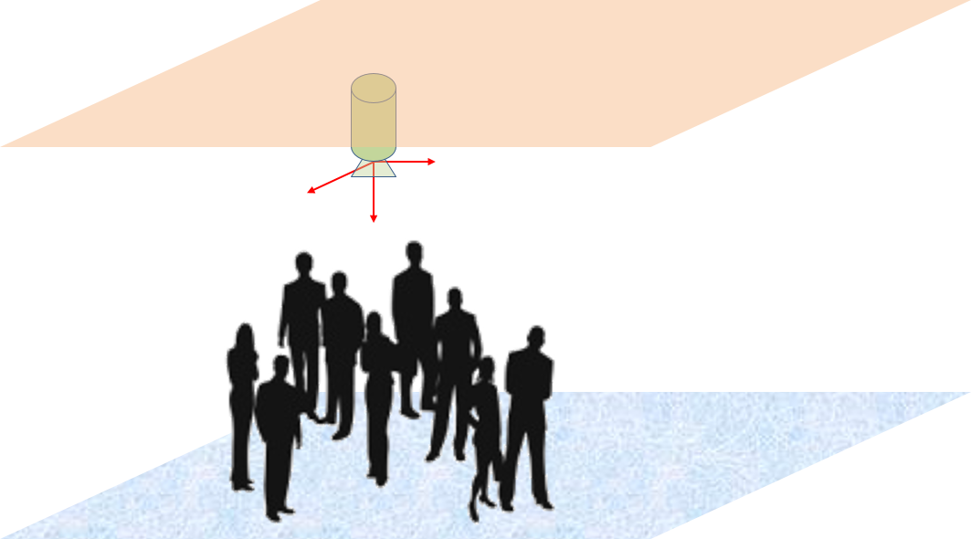
(a) Camera location above sensed area.

(b) Example of recorded frame in sensed area.

Figure 1: Scheme of camera location above sensed area and example of recorded frame

The structure of the paper is described as follows: section 2 describes the person detection algorithm, section 3 includes the experimental setup, results and discussion, and section 4 contains the main conclusions and some ideas for future work.

2 DPDnet People Detector

2.1 Problem Formulation

We propose the DPDnet neural network to detect multiple people from a single depth image. The output consists of a multi-modal confidence map, the same size as the input image, that jointly codifies the detection of multiple people in scene (see Figure 2).

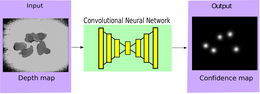
Figure 2: Depth input image and output confidence map.

.

The confidence map assigns a 2D Gaussian distribution centered in each detected person. We use the centroid of the head in image coordinates as the localization reference. The 2D position of each person can be easily obtained from the confidence map by detecting its local maxima.

The advantages of this strategy are twofold: first, learning the confidence map is a well defined process to detect multiple hypothesis as opposed to using other parametrizations (e.g multiple 2D coordinate vectors) which can lead to ambiguities in the regression function. Second, it makes computational complexity to be independent from the number of people in the scene, assuming that the time used for extracting multiple detection hypotheses from the confidence map is mostly negligible.

2.2 DPDnet Network Architecture

Figure 3 illustrates our approach to detect people from a single depth image.

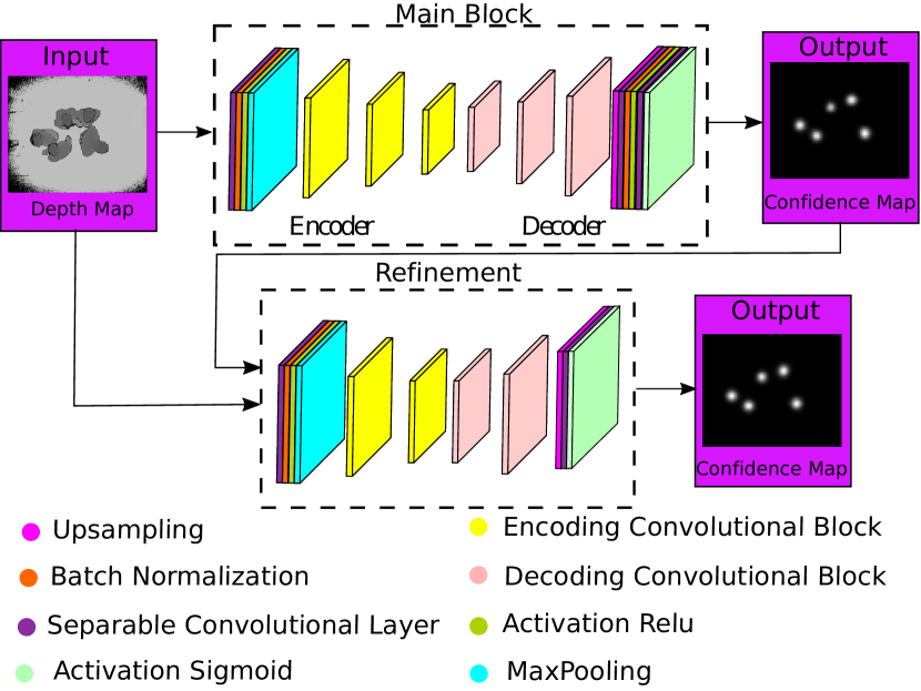
Figure 3: The DPDnet architecture divided into the main block and the refinement block. Figure shows the general encoder-decoder structure in both blocks.

.

Our DPDnet neural network consists of two blocks: the main block and the refinement block. Both blocks use the encoder-decoder architecture inspired in the Segnet [4] model, originally proposed in semantic segmentation, and use the residual layers proposed in the ResNet [18] model.

The main block takes a single depth image as input, and outputs a confident map. The refinement block takes as inputs the input depth image along with the confidence map obtained from the main block, and outputs a refined confidence map. In Section 3, we show that the refinement block significantly outperforms the results obtained by the main block alone. Similar refinement blocks have been proposed for other tasks, such as in monocular reconstruction methods [monocular_reconstruction].

The structure of the main block is detailed in Table 3. It takes $212\times 256$ depth images as input, and uses separable convolutional layers based on the Xception [11] model. Separable convolutions are faster than conventional convolutions, while achieving similar performance. In addition to this, we use ReLU activations [1] and batch normalization. To build the encoder-decoder core of the main block, we use several units of residual blocks, similar to those proposed in the ResNet [18] model. Encoding blocks downsample the spatial dimensions by a factor of two, and decoding blocks use upscaling layers to increase the spatial dimensions by the same factor. Their basic architecture is described in Figure 4 and Tables 1 and 2.

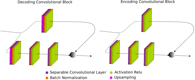
Figure 4: DPDnet decoding and encoding block.

Table 1: Encoding Block

Encoding Block (filters=(a,b,c)),kernel size=k
Layer	Parameters	Output Size
Input	-	(Width, Height, Depth)
Convolution (Main Branch)	kernel=(1, 1) strides=(2, 2) filters=a	(Width/2, Height/2, a)
Batch Normalization (Main Branch)	-
Activation (Main Branch)	ReLU
Convolution (Main Branch)	kernel=(k, k) strides=(1, 1) filters=b	(Width/2, Height/2, b)
Batch Normalization (Main Branch)	-
Activation (Main Branch)	ReLU
Convolution (Main Branch)	kernel=(1, 1) strides=(1, 1) filters=c	(Width/2, Height/2, c)
Batch Normalization (Main Branch)	-
Convolution (Shortcut)	kernel=(1, 1) strides=(2, 2) filters=c	(Width/2, Height/2, c)
Batch Normalization (Shortcut)	-
Add (Main Branch+Shortcut)	-	(Width/2, Height/2, a)
Activation (Main Branch+Shortcut)	ReLU

Table 2: Decoding Block

Decoding Block (filters=(a,b,c)),kernel size=k
Layer	Parameters	Output Size
Input	-	(Width, Height, Depth)
Upsampling (Main Branch)	size=(2,2)	(2*Width,2*Height,Depth)
Convolution (Main Branch)	kernel=(1, 1) strides=(1, 1) filters=a	(Width/2, Height/2, a)
Batch Normalization (Main Branch)	-
Activation (Main Branch)	ReLU
Convolution (Main Branch)	kernel=(k, k) strides=(1, 1) filters=b	(Width/2, Height/2, b)
Batch Normalization (Main Branch)	-
Activation (Main Branch)	ReLU
Convolution (Main Branch)	kernel=(1, 1) strides=(1, 1) filters=c	(Width/2, Height/2, c)
Batch Normalization (Main Branch)	-
Upsampling (Shortcut)	size=(2,2)	(2*Width,2*Height,Depth)
Convolution (Shortcut)	kernel=(1, 1) strides=(1, 1) filters=c	(Width/2, Height/2, c)
Batch Normalization (Shortcut)	-
Add (Main Branch+Shortcut)	-	(Width/2, Height/2, a)
Activation (Main Branch+Shortcut)	ReLU

Finally, the last block of the CNN and the cropping layers adapt the output of the last decoding block to the output size of the confidence map ($212\times 256$), which is the same size as the input image. Table 3 summarizes all layers that appear in the main block.

Table 3: Main Stage. In Encoding and Decoding Blocks, a, b and c represents the number of filters of the intermediate convolutional layers in the branches.

Main Block
Layer	Output Size	Parameters
Input	212x256x1	-
Convolution	106x128x64	kernel=(7, 7) / strides=(2, 2)
Batch Normalization	-
Activation	ReLU
Max Pooling	35x42x64	size=(3, 3)
Encoding Conv. Block	35x42x256	kernel=(3, 3) / strides=(1, 1) (a=64, b=64, c=256)
Encoding Conv. Block	18x21x512	kernel=(3, 3) / strides=(2, 2) (a=128, b=128, c=512)
Encoding Conv. Block	9x11x1024	kernel=(3, 3) / strides=(2, 2) (a=256, b=256, c=1024)
Decoding Separable Conv. Block	9x11x256	kernel=(3, 3) / strides=(1, 1) (a=1024, b=1024, c=256)
Decoding Separable Conv. Block	18x22x128	kernel=(3, 3) / strides=(2, 2) (a=512, b=512, c=128)
Decoding Separable Conv. Block	36x44x64	kernel=(3, 3) / strides=(2, 2) (a=256, b=256, c=64)
Cropping	36x43x64	cropping=[(2, 2) (1, 1)]
Up Sampling	108x129x64	size=(3, 3)
Convolution	216x258x64	kernel=(7, 7) / strides=(2, 2)
Cropping	212x256x64	cropping=[(2, 2) (1, 1)]
Batch Normalization	-
Activation	ReLU
Convolution	212x256x1	kernel=(3, 3) / strides=(1, 1)
Activation	Sigmoid
Output 1	212x256x1	-

The refinement stage is a reduced version of the main block with two encoding and decoding blocks. It is thus more shallow than the main block. The refinement block takes as inputs the input depth image and the confidence map computed from the main block, and outputs a new “refined” confidence map. Table 4 summarizes all the layers and blocks used in the refinement stage.

Table 4: Refinement Stage

Refinement Block
Layer	Output Size	Parameters
Output 1 + Input	212x256x1	-
Convolution	106x128x64	kernel=(7, 7) / strides=(2, 2)
Batch Normalization	-
Activation	ReLU
Max Pooling	35x42x64	size=(3, 3)
Encoding Conv. Block	35x42x256	kernel=(3, 3) / strides=(1, 1) (a=64, b=64, c=256)
Encoding Conv. Block	18x21x512	kernel=(3, 3) / strides=(2, 2) (a=128, b=128, c=512)
Decoding Conv. Block	36x42x128	kernel=(3, 3) / strides=(2, 2) (a=512, b=512, c=128)
Decoding Conv. Block	72x84x64	kernel=(3, 3) / strides=(2, 2) (a=256, b=256, c=64)
Zero Padding	72x86x64	padding=(0, 1)
Up Sampling	216x258x64	size=(3, 3)
Cropping	212x256x64	cropping=[(2, 2) (1, 1)]
Convolution	212x256x1	kernel=(3, 3) / strides=(1, 1)
Activation	Sigmoid
Output 2	212x256x1	-

In addition to the DPDnet architecture described above, we have adapted the same model to work with images half the resolution of the original ones ($106\times 128$), seamlessly producing downscaled confident maps. We will refer to this reduced model as DPDnet_fast in section 3. The reduction of input and output size allows low cost GPUs to run our model with a very small impact in terms of accuracy.

2.3 Training procedure

We denote by $p_{i}$ the input depth image and by $q_{i}$ the target confident map, where $p_{i},q_{i}\in\mathbb{R}^{212\times 256}$. We assume that both $p_{i}$ and $q_{i}$ are normalized in the interval $[0,1]$. The target confidence map $q_{i}$ is generated by a sum of two-dimensional Gaussian distributions with covariance matrix $P=\sigma^{2}\mathbb{I}_{2\times 2}$ and centered around the labeled position of each person in the scene. We use $\sigma=6$ pixels in all our experiments.

The main and refinement blocks of the DPDnet are defined with the functions $\mathcal{T}_{m}(p_{i},\theta_{m})$ and $\mathcal{T}_{r}(p_{i},q_{i},\theta_{r})$ respectively. All trainable parameters of the main block are defined with vector $\theta_{m}$, and similarly with $\theta_{r}$ for the refinement block. When referring to all trainable parameters of the entire DPDnet model we use their concatenation $\theta=(\theta_{m},\theta_{r})$.

The complete DPDnet function $\mathcal{T}(p_{i},\theta)$ is obtained by composition of $\mathcal{T}_{m}$ and $\mathcal{T}_{r}$:

$$\mathcal{T}(p_{i},\theta)=\mathcal{T}_{r}\left(p_{i},\mathcal{T}_{m}(p_{i},\theta_{m}),\theta_{r}\right)$$ (1)

We train our network using a set of corresponding depth images and confidence maps $\{(p_{i},q_{i})\}_{i=1,\dots,N}$. The following loss function is used:

$$\mathcal{L}(\theta)=\frac{1}{N}\sum_{i=1}^{N}\|\mathcal{T}(p_{i},\theta)-q_{i}\|^{2}+\lambda\frac{1}{N}\sum_{i=1}^{N}\|\mathcal{T}_{m}(p_{i},\theta_{m})-q_{i}\|^{2},$$ (2)

where $\lambda$ is a hyper-parameter that weights the importance of the two terms in the loss function and is set to $\lambda=1$ in our experiments. Note that the second term of equation (2) imposes the main block to be as close as possible to the target confidence map. This forces the refinement block to improve the output of the main block.

By minimizing equation (2), we train the entire DPDnet model end-to-end in a single step without separating the main block and refinement block.

In our experiments, we train the network for $50$ epochs and use a validation set to select the best model. We employ the Adam optimizer [22] with $0.001$ as initial learning rate. This optimizer has been chosen because of its adaptive capabilities in terms of learning rate. The great advantage of Adam is the fact that it starts from an initial learning rate set by the user and then uses the first and second moments of the gradient to adapt the learning rate to the situation stipulated by Adam in the loss function. This provides unrivaled speed and robustness compared to other optimizers, making Adam a good choice for the problem proposed here.

3 Experimental Work

3.1 Datasets

In order to provide a wide range of evaluation conditions, we have used three different databases, that will be described next. Figure 5 provides some sample frames to give an idea on the style and quality of the different datasets.

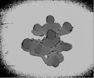
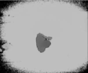
(a) Sample frames from the GOTPD1+ dataset.

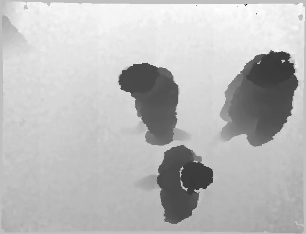
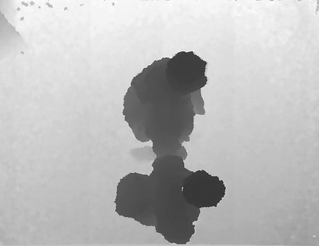
(b) Sample frames from the MIVIA dataset.

(c) Sample frames from the Zhang2012 dataset.

Figure 5: Sample frames from the databases used (gray coded depth).

3.1.1 GOTPD1 database

In this work, we have used part of the GOTPD1 database (available at [27] and GOTPD1, that was recorded with a Kinect^® v2 device located at a height of $3.4m$. The recordings covered a broad variety of conditions, with scenarios comprising single and multiple people, single and multiple non-people (such as chairs), people with and without accessories (hats, caps), people with different complexity, height, hair color, and hair configurations, people actively moving and performing additional actions (such as using their mobile phones, moving their fists up and down, moving their arms, etc.).

The GOTPD1 data was originally split in two subsets, one for training and the other for testing, with the configuration described in [26]. However, for this work, and given the strict training data requirements of deep learning approaches, we will be using the full GOTPD1 dataset for training purposes, and we recorded 23 additional sequences to allow for a proper evaluation effort. In this manner, the training and testing subsets are fully independent, as people and conditions differ between training and testing recordings.

Table 5 and Table 6 show the details of the training and testing subsets, respectively. #Frames refers to the number of frames in the recorded sequences, while #Positives refers to the number of all the heads over all the frames (in our recordings we used 39 different people). The database contains sequences in which the users were instructed on how to move under the camera (to allow for proper coverage of the recording area), and sequences where people moved freely (to allow for a more natural behavior).

Table 5: GOTPD1+ Training subset details.

$\#Sequences$	$\#Frames$	$\#Positives$	Description
S0001 through S0022, S0102,S0110,S0123, S0130,S0136,S0142	$26853$	$14381$	Single people sequences
S0023 through S0026	$7138$	$2416$	Two people sequences
S0027 through S0029, S0031 through S0034, S0152, S0153	$6526$	$18106$	Multiple people sequences
S0035, S0038 through S0040	$2323$	$1458$	Sequences with chairs and people balancing fists facing up
Totals	$42840$	$36361$

Table 6: GOTPD1+ testing subset details.

Sequence IDs	$\#Samples$	$\#Positives$	Description
S041, S0101, S0131 through S0135, S143	$2742$	$2391$	Single people sequences
S0144 through S0146	$1888$	$2865$	Two people sequences
S0030, S0147 through S0151, S0154 through 157	$4516$	$14837$	Multiple people sequences
S0036 through S0037	$1789$	$0$	Sequences with chairs
Totals	$11375$	$21403$

This dataset (composed by the original GOTPD1 and the additional 23 recorded sequences), will be referred to as GOTPD1+ in the tables included in Section 3.4. The first row of figure 5 shows two sample frames from this dataset.

3.1.2 MIVIA People Counting Dataset

The MIVIA people counting dataset (available at [24]) has been developed by the MIVIA Research Lab in the University of Palermo and was first described and used in [13]. It is mainly aimed at evaluating people flow density in the sensed environment, but we will use it for people counting and tracking purposes.

The MIVIA dataset includes RGB and depth data captured with a Kinect^® device located in an overhead position at a height of $3.20m$. The recordings have been captured in indoor and outdoor conditions, and for isolated and group transits. From the 34 available sequences, we will be using 8 of them, all that correspond to indoor conditions for both the single people and multiple people transits. The recordings include people walking with bags and other big objects, and their details are shown in Figure 7.

Table 7: MIVIA testing subset details.

Sequence IDs	$\#Frames$	$\#Positives$	Description
DIS1 DIS2	7692	3601	Single people sequences
DIS3 DIS4 DIS5	10259	5315	Two people sequences
DIG1 DIG2 DIG3	12222	8780	Multiple people sequences
Totals	30173	17696

In our experiments we will use the depth streams with a resolution of ${640\times 480}$. Because of the different sizes, it will be necessary to resize the depth streams used in this database to the sizes that DPDnet can use.

This dataset will be referred to as MIVIA in the tables included in Section 3.4. Middle row of figure 5 shows two sample frames from this dataset.

3.1.3 Zhang 2012 database

The Zhang 2012 database [43] consists of two sequences (dataset1 and dataset2) recorded with a Kinect^® device also located in an overhead position, generating depth data with a resolution of $320\times 240$ pixels. Both sequences include multiple people moving under the camera, and their details are shown in Table 8. The recordings include groups of people walking closely to each other, people walking freely and people with bags and other big objects.

The data, kindly provided to us by its authors, is processed with an ad-hoc background subtraction strategy (described in [43]), that induces some artifacts in the depth images.

Table 8: Zhang2012 testing subset details.

Sequence IDs	$\#Positives$	$\#Positives$	Description
dataset1	2384	4527	Multiple people sequences
dataset2	1500	1553	Multiple people sequences
Totals	3884	6080

This dataset will be referred to as Zhang2012 in the tables included in section 3.4. Last row of figure 5 shows two sample frames from this dataset.

3.2 Experimental setup

In all the experiments carried out, we use the three different datasets described in section 3.1.

We compare the performance of our proposals DPDnet and DPDnet_fast with other strategies described in the literature that use an overhead ToF camera in a people detection/tracking/counting task. The following state-of-the-art methods are used for comparison:

• WaterFilling [43]: this method is based on the water filling algorithm and the original source code was kindly provided to us by its authors. To run this method in the GOTPD1+ dataset we scaled the images to $640\times 480$ pixels.

• SLICE_PCA [26]: this method uses feature vectors extracted from the depth image and a generative PCA model of these vectors to classify detections. In our experiments, the PCA model is trained using the GOTPD1 dataset. In this regard, we train two categories: people and non-people.

• SLICE_SVM [15]: this method is similar to SLICE_PCA, but uses a SVM classifier instead of PCA. In our experiments, the SVM model is trained again using the full GOTPD1 dataset.

• MexicanHat [35, 36]: this method is based on the normalized Mexican Hat Wavelet and requires the detection and removal of the floor plane. It does not require training data though.

It is important to note that in the comparison, we did not use a tracking module for any of the methods. Our objective is to provide a fair comparison on their discrimination capabilities without other improvements. The only input frame manipulation we did was that required to scale the frame size to fit in the input stage conditions of the evaluated algorithms.

3.3 Evaluation Metrics

To provide a detailed view on the performance on the evaluated algorithms, we will calculate the main standard metrics in a detection problem, namely: $Precision$, $Recall$, $F1_{score}$, False Negative Rate ($FNR$), False Positive Rate ($FPR$), and overall error $ERR$ (calculated as $ERR=FNR+FPR$)

We will also calculate confidence intervals for the $F1_{score}$ and $ERR$ metrics, for a confidence value of $95\%$, to assess the statistical significance of the results when comparing different strategies.

3.4 Results and Discussion

In this section we will first provide detailed results for all the algorithms described in Section 3.2 applied to each of the datasets described in Section 3.1.

Tables 9, 10 and 11 include the results for the GOTPD1+,MIVIA and Zhang2012 datasets respectively, including the evaluation metrics described in section 3.3 for all the evaluated algorithms. To visually aid in the analysis of the results, we have added a green background to those table cells that correspond to the best results across all algorithms for each condition.

Table 9: Detailed Results using all the tested algorithms on the GOTPD1+ dataset. All values in $\%$ (cells in green background correspond to the best results across all algorithms for each condition).

	DB	$Precision$	$Recall$	$F1_{score}$	$FNR$	$FPR$	$ERR$
MexicanHat	Single person	$99.87$	$99.34$	$99.60\pm 0.23$	$0.66$	$0.16$	$0.44\pm 0.25$
	Two people	$99.63$	$49.72$	$66.34\pm 1.91$	$50.28$	$0.41$	$34.84\pm 1.93$
	More than two people	$99.86$	$37.84$	$54.88\pm 0.87$	$62.16$	$0.47$	$55.92\pm 0.87$
	Chairs. no people					$21.97$	$21.97\pm 1.92$
	Totals	$94.24$	$45.63$	$61.48\pm 0.68$	$54.37$	$8.06$	$42.48\pm 0.69$
SLICESVM	Single person*	$98.23$	111 $\mathbf{99.87}$	$99.04\pm 0.36$	111 $\mathbf{0.13}$	$2.18$	$1.06\pm 0.38$
	Two people*	$93.17$	111 $\mathbf{100.00}$	$96.46\pm 0.75$	111 $\mathbf{0.00}$	$16.25$	$5.05\pm 0.89$
	More than two people*	$99.93$	$99.26$	$99.59\pm 0.11$	$0.74$	$0.63$	$0.73\pm 0.15$
	Chairs. no people*					$35.33$	$35.33\pm 2.21$
	Totals*	$96.71$	$99.40$	$98.04\pm 0.19$	$0.60$	$9.70$	$2.95\pm 0.24$
SLICEPCA	Single person	$98.23$	111 $\mathbf{99.87}$	$99.04\pm 0.36$	111 $\mathbf{0.13}$	$2.18$	$1.06\pm 0.38$
	Two people	$94.10$	111 $\mathbf{100.00}$	$96.96\pm 0.70$	111 $\mathbf{0.00}$	$13.91$	$4.32\pm 0.82$
	More than two people	$99.93$	$99.20$	$99.56\pm 0.12$	$0.80$	$0.63$	$0.79\pm 0.15$
	Chairs. no people					$0.00$	111 $\mathbf{0.00}\pm 0.00$
	Totals	$99.06$	$99.36$	$99.21\pm 0.12$	$0.64$	$2.70$	$1.18\pm 0.15$
WaterFilling	Single person	$98.18$	$98.63$	$98.40\pm 0.47$	$1.37$	$2.31$	$1.79\pm 0.50$
	Two people	$99.26$	111 $\mathbf{100.00}$	$99.63\pm 0.25$	111 $\mathbf{0.00}$	$1.66$	$0.51\pm 0.29$
	More than two people	$99.90$	$99.81$	$99.85\pm 0.07$	$0.19$	$0.86$	$0.26\pm 0.09$
	Chairs. no people					$22.97$	$22.97\pm 1.95$
	Totals	$96.90$	$99.70$	$98.28\pm 0.18$	$0.30$	$9.24$	$2.59\pm 0.22$
DPDnetfast	Single person	222 $\mathbf{100.00}$	$99.67$	$99.84\pm 0.15$	$0.33$	222 $\mathbf{0.00}$	$0.18\pm 0.16$
	Two people	$99.88$	222 $\mathbf{100.00}$	$99.94\pm 0.10$	222 $\mathbf{0.00}$	$0.28$	$0.09\pm 0.12$
	More than two people	$99.92$	222 $\mathbf{99.90}$	222 $\mathbf{99.91}\pm 0.05$	$0.10$	$0.71$	222 $\mathbf{0.16}\pm 0.07$
	Chairs. no people					$0.39$	$0.39\pm 0.29$
	Totals	$99.88$	222 $\mathbf{99.89}$	222 $\mathbf{99.88}\pm 0.05$	222 $\mathbf{0.11}$	$0.36$	222 $\mathbf{0.17}\pm 0.06$
DPDnet	Single person	$99.93$	222 $\mathbf{99.87}$	222 $\mathbf{99.90}\pm 0.12$	222 $\mathbf{0.13}$	$0.08$	222 $\mathbf{0.11}\pm 0.12$
	Two people	222 $\mathbf{100.00}$	$99.94$	222 $\mathbf{99.97}\pm 0.07$	$0.06$	222 $\mathbf{0.00}$	222 $\mathbf{0.04}\pm 0.08$
	More than two people	222 $\mathbf{100.00}$	$99.71$	$99.86\pm 0.07$	$0.29$	222 $\mathbf{0.00}$	$0.26\pm 0.09$
	Chairs. no people					222 $\mathbf{0.00}$	222 $\mathbf{0.00}\pm 0.00$
	Totals	222 $\mathbf{99.99}$	$99.75$	$99.87\pm 0.05$	$0.25$	222 $\mathbf{0.02}$	$0.19\pm 0.06$

3.4.1 Results for the GOTPD1+ database

Regarding the results for the GOTPD1+ database (Table 9), it is clearly seen that the DPDnet and DPDnet_fast solutions are the best ones, and this is specially significant for sequences including more than two people. Despite this, SLICE_PCA and SLICE_SVM also obtain top results for the $Recall$ and $FNR$ rates, for the sequences with one and two people. This happens at the cost of significantly increase the $FPR$ rates, which is the reason why these methods finally got worse performance in the $F1_{score}$ and $ERR$ metrics. The WaterFilling algorithm has also top performance for the sequences with two people, but also with higher $FPR$ rates. The MexicanHat algorithm is clearly the worst one, as has been already proved in previous works.

Despite the good results of SLICE_SVM and WaterFilling, their robustness to sequences without people (just chairs) is less than that of DPDnet, SLICE_PCA and DPDnet_fast. In the case of SLICE_SVM, this bad performance could be due to the class modeling carried out, and for the WaterFilling algorithm, it is clearly due to the absence of an explicit discrimination procedure, which generates a higher number of false positives. The results obtained with the SLICE_PCA method in the chair sequences are similar or better than those obtained with our CNN based proposals, but we must bear in mind that the SLICE_PCA method requires a calibration process to know the intrinsic and extrinsic parameters of the sensor.

It is also worth mentioning that the DNN based methods are undoubtedly the best when considering the $FPR$ rates, showing a very good discrimination capability.

Finally, when comparing DPDnet and DPDnet_fast, a singular effect can be observed: the $FNR$ values for DPDnet_fast are better than those of DPDnet, while the $FPR$ values of DPDnet are better than those of DPDnet_fast. This can be explained by the reduction in the image resolution, since this reduction implies an interpolation that allows to slightly filter the noise and artifacts in the input image. This can lead the fast version to have an easier job in discriminating negatives, while in the case of the conventional version, the availability of the full image information allows for a better discrimination of actual people present in the scene.

Table 10: Detailed Results using all the tested algorithms on the MIVIA dataset. All values in $\%$ (cells in green background correspond to the best results across all algorithms for each condition).

	DB	$Precision$	$Recall$	$F1_{score}$	$FNR$	$FPR$	$ERR$
MexicanHat	Single person	$93.76$	$92.66$	$93.21\pm 0.56$	$7.34$	$2.94$	$4.36\pm 0.46$
	Two people	$88.61$	$86.64$	$87.61\pm 0.64$	$13.36$	$6.21$	$8.77\pm 0.55$
	More than two people	$93.73$	$53.67$	$68.26\pm 0.76$	$46.33$	$2.65$	$21.21\pm 0.67$
	Totals	$91.81$	$71.40$	$80.33\pm 0.43$	$28.60$	$3.89$	$13.27\pm 0.37$
SLICESVM	Single person*	$92.92$	$93.90$	$93.41\pm 0.55$	$6.10$	$3.39$	$4.26\pm 0.45$
	Two people*	$87.75$	$87.97$	$87.86\pm 0.63$	$12.03$	$6.85$	$8.70\pm 0.55$
	More than two people*	$91.85$	$94.11$	$92.96\pm 0.42$	$5.89$	$6.13$	$6.03\pm 0.39$
	Totals*	$90.85$	$92.22$	$91.53\pm 0.30$	$7.78$	$5.66$	$6.46\pm 0.27$
SLICEPCA	Single person*	$93.30$	$93.90$	$93.67\pm 0.55$	$6.10$	$3.20$	$4.13\pm 0.44$
	Two people*	$87.97$	$87.97$	$87.97\pm 0.63$	$12.03$	$6.71$	$8.62\pm 0.54$
	More than two people*	$92.91$	$93.95$	$93.43\pm 0.40$	$6.05$	$5.25$	$5.59\pm 0.38$
	Totals*	$91.52$	$92.14$	$91.83\pm 0.30$	$7.86$	$5.20$	$6.20\pm 0.26$
WaterFilling	Single person	$95.20$	222$\mathbf{98.96}$	$97.04\pm 0.38$	222$\mathbf{1.04}$	$2.41$	$1.96\pm 0.31$
	Two people	$96.67$	222$\mathbf{99.84}$	$98.23\pm 0.26$	222$\mathbf{0.16}$	$1.96$	$1.31\pm 0.22$
	More than two people	$91.29$	222$\mathbf{98.53}$	$94.77\pm 0.37$	222$\mathbf{1.47}$	$6.81$	$4.57\pm 0.34$
	Totals	$93.68$	222$\mathbf{99.02}$	$96.27\pm 0.21$	222$\mathbf{0.98}$	$4.08$	$2.91\pm 0.18$
DPDnetfast	Single person	$99.71$	$97.41$	$98.55\pm 0.27$	$2.59$	$0.14$	$0.94\pm 0.22$
	Two people	$99.54$	$99.09$	$99.32\pm 0.16$	$0.91$	$0.26$	$0.50\pm 0.14$
	More than two people	222$\mathbf{99.24}$	$96.62$	$97.91\pm 0.23$	$3.38$	222$\mathbf{0.53}$	$1.72\pm 0.21$
	Totals	$99.43$	$97.54$	$98.47\pm 0.13$	$2.46$	$0.34$	$1.14\pm 0.12$
DPDnet	Single person	222$\mathbf{100.00}$	$98.56$	222$\mathbf{99.27}\pm 0.19$	$1.44$	222$\mathbf{0.00}$	222$\mathbf{0.47}\pm 0.15$
	Two people	222$\mathbf{99.81}$	$99.05$	222$\mathbf{99.43}\pm 0.15$	$0.95$	222$\mathbf{0.11}$	222$\mathbf{0.41}\pm 0.12$
	More than two people	$99.23$	$98.14$	222$\mathbf{98.68}\pm 0.19$	$1.86$	$0.54$	$1.09\pm 0.17$
	Totals	222$\mathbf{99.57}$	$98.50$	222$\mathbf{99.03}\pm 0.11$	$1.50$	222$\mathbf{0.26}$	222$\mathbf{0.72}\pm 0.09$

3.4.2 Results for the MIVIA database

Regarding the results for the MIVIA database (Table 10), we first have to stress and remind the fact that no training nor adaptation has been done for this new dataset.

Again, the best results are found in the CNN-based methods (which imply the use of a model trained on a different dataset), and (in specific metrics) in the WaterFilling algorithm (that does not need any training procedure).

The SLICE_PCA and SLICE_SVM methods exhibit a relevant performance drop that can be explained by their higher sensitivity to the mismatch in the recording conditions as compared with those of the training material used.

The better performance of the WaterFilling algorithm in the $Recall$ and $FNR$ rates is again achieved at the cost of increasing the $FPR$ rates, which finally translates to overall lower $F1_{score}$ and $ERR$ metrics.

As in the case of GOTPD1+, the MexicanHat method is the worst of all in all metrics.

Table 11: Detailed Results using all the tested algorithms on the Zhang2012 dataset. All values in $\%$ (cells in green background correspond to the best results across all algorithms for each condition).

	DB	$Precision$	$Recall$	$F1_{score}$	$FNR$	$FPR$	$ERR$
MexicanHat	Dataset1	$40.52$	$24.51$	$30.54\pm 1.51$	$75.49$	$410.76$	$102.49\pm-$
	Dataset2	$26.72$	$21.02$	$23.53\pm 2.02$	$78.98$	$86.32$	$81.92\pm 1.83$
	Totals	$36.56$	$23.68$	$28.74\pm 1.22$	$76.32$	$182.85$	$95.87\pm 0.54$
SLICESVM	Dataset1*	$82.92$	$85.77$	$84.32\pm 1.19$	$14.32$	$226.82$	$29.60\pm 1.49$
	Dataset2*	$59.56$	$59.28$	$59.42\pm 2.33$	$40.72$	$64.38$	$49.82\pm 2.37$
	Totals*	$77.50$	$79.44$	$78.46\pm 1.10$	$20.56$	$110.57$	$36.09\pm 1.29$
SLICEPCA	Dataset1*	$94.31$	$97.81$	$96.03\pm 0.64$	$2.19$	$67.60$	$7.44\pm 0.86$
	Dataset2*	$94.48$	$99.30$	$96.83\pm 0.83$	$0.70$	$8.36$	$3.84\pm 0.92$
	Totals*	$94.35$	$98.16$	$96.22\pm 0.52$	$1.84$	$25.69$	$6.28\pm 0.66$
WaterFilling	Dataset1	$95.40$	$98.76$	$97.05\pm 0.55$	$1.24$	$55.48$	$5.53\pm 0.75$
	Dataset2	$96.70$	$98.91$	$97.79\pm 0.70$	$1.09$	$4.96$	$2.66\pm 0.77$
	Totals	$95.70$	$98.79$	$97.22\pm 0.44$	$1.21$	$19.71$	$4.61\pm 0.57$
DPDnetfast	Dataset1	222$\mathbf{99.57}$	$99.21$	222$\mathbf{99.39}\pm 0.25$	$0.79$	222$\mathbf{4.95}$	222$\mathbf{1.12}\pm 0.34$
	Dataset2	222$\mathbf{99.01}$	$99.11$	222$\mathbf{99.06}\pm 0.46$	$0.89$	222$\mathbf{1.45}$	222$\mathbf{1.12}\pm 0.50$
	Totals	222$\mathbf{99.44}$	$99.19$	222$\mathbf{99.31}\pm 0.22$	$0.81$	222$\mathbf{2.47}$	222$\mathbf{1.12}\pm 0.28$
DPDnet	Dataset1	$98.89$	222$\mathbf{99.76}$	$99.32\pm 0.27$	222$\mathbf{0.24}$	$12.94$	$1.26\pm 0.36$
	Dataset2	$97.10$	222$\mathbf{99.90}$	$98.48\pm 0.58$	222$\mathbf{0.10}$	$4.35$	$1.83\pm 0.64$
	Totals	$98.46$	222$\mathbf{99.79}$	$99.12\pm 0.25$	222$\mathbf{0.21}$	$6.87$	$1.44\pm 0.32$

3.4.3 Results for the Zhang2012 database

Regarding the results for the Zhang2012 database (Table 11), we are again in the case of a mismatch between the training and evaluation conditions discussed above.

Here, the superiority of the CNN-based methods are even clearer than in the two previous datasets, obtaining very good results considering the experimental conditions.

The performance drop of the SLICE_PCA and SLICE_SVM methods is higher than in the MIVIA results (specially in the latter). As mentioned in Section 3.1.3, images of this dataset contain artifacts from the background subtraction method, and this might affect the classifiers SLICE_PCA and SLICE_SVM, which were trained with cleaner data.

As discussed in the case of the MIVIA results, the WaterFilling algorithm performance is closer to the top results in the $Recall$ and $FNR$ rates, with the same explanation than above.

The CNN-based methods are affected by image artifacts to a much lower extent than SLICE_PCA and SLICE_SVM. Between the two proposals, DPDnet is more affected than DPDnet_fast, possibly given that its greater number of parameters (due to its the larger input image size) forces it to search for more defined and detailed features similar to those found in the training subset of the GOTPD1+ dataset, while DPDnet_fast generalizes better when facing new datasets, due to the lower definition of its input images (finding more general characteristics of people).

Finally, as in all the previous cases, the MexicanHat method gets the worst performance for all metrics.

3.4.4 Overall comparison

Once the detailed results have been discussed for each dataset, now we will provide full details on the overall comparison among the evaluated algorithms for all the datasets used. We will include tables with the overall behavior of the different strategies, and we will also include bar charts to ease the visual comparison, providing error confidence values for all the metrics. In the tables and graphics below, we have omitted the results for the MexicanHat algorithm due to its bad performance. In the charts, please note that the vertical scale is not the same for all of them, as they have been adjusted to allow for a better visualization.

From the previous discussion on the results show in tables 9, 10 and 11, it can be concluded that the proposed solutions DPDnet and DPDnet_fast are the best alternatives for a robust detection in this application. They have obtained the best results, and they have proved to be robust against changing database recording conditions, maintaining the overall error rate around $1\%$ percent in all cases. The classic trainable methods such as SLICE_PCA and SLICE_SVM are good alternatives but have worse results, and they require calibration and retraining to change the detection environment to provide optimal results. On the other hand, WaterFilling can be seen as another alternative system, but unlike the two previous approaches, it acts more as a detector of maximums than as a classification algorithm. Finally, the MexicanHat algorithm is not a good alternative system and globally has obtained the worst results among the evaluated systems.

Table 12 shows the final aggregated results of the evaluated algorithms on the GOTPD1+ dataset, and in Figures 6(a) and 6(b) we show the graphical comparison among the different strategies.

Table 12: Results for the GOTPD1+ dataset. All values in $\%$.

DB	$Precision$	$Recall$	$F_{1}score$	$FNR$	$FPR$	$ERR$
DPDnet	222$\mathbf{99.99}$	$99.75$	$99.87\pm 0.05$	$0.25$	222$\mathbf{0.02}$	$0.19\pm 0.06$
DPDnetfast	$99.88$	222$\mathbf{99.89}$	222$\mathbf{99.88}\pm 0.05$	222$\mathbf{0.11}$	$0.36$	222$\mathbf{0.17\pm 0.06}$
WaterFilling	$96.90$	$99.70$	$98.28\pm 0.18$	$0.30$	$9.24$	$2.59\pm 0.22$
SLICEPCA*	$99.06$	$99.36$	$99.21\pm 0.12$	$0.64$	$2.70$	$1.18\pm 0.15$
SLICESVM*	$96.71$	$99.40$	$98.04\pm 0.19$	$0.60$	$9.70$	$2.95\pm 0.24$
MexicanHat	$94.24$	$45.63$	$61.48\pm 0.68$	$54.37$	$8.06$	$42.48\pm 0.69$

Figure 6(a) shows how the performance metrics are reasonably high, except for the WaterFilling and SLICE_SVM algorithms, whose $Precision$ and $F1_{score}$ have a significant drop. This tendency is also clearly observed in the error metrics of Figure 6(b). The CNN-based methods achieve the best results, and the observed improvements are statistically significant against the non CNN-based methods, considering the included confidence bands.

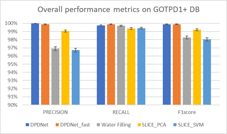
(a) Performance metrics.

.

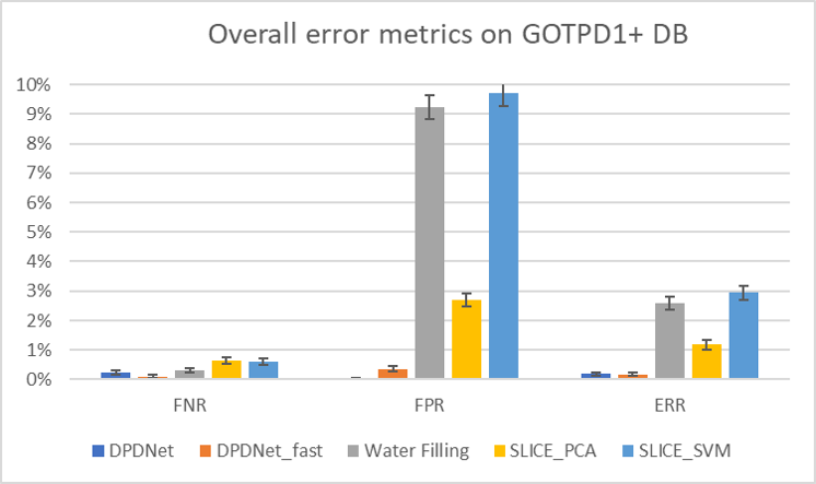
(b) Error metrics.

.

Figure 6: Overall performance and error metrics for the GOTPD1+ dataset.

Table 13 shows the final aggregated results of the evaluated algorithms on the MIVIA dataset, and in Figures 7(a) and 7(b) we show the graphical comparison among the different strategies

Table 13: Results for the MIVIA dataset. All values in $\%$.

DB	$Precision$	$Recall$	$F_{1}score$	$FNR$	$FPR$	$ERR$
DPDnet	222$\mathbf{99.57}$	222$\mathbf{98.50}$	222$\mathbf{99.03\pm 0.11}$	222$\mathbf{1.50}$	222$\mathbf{0.26}$	222$\mathbf{0.72\pm 0.09}$
DPDnetfast	$99.43$	$97.54$	$98.47\pm 0.13$	$2.46$	$0.34$	$1.14\pm 0.12$
WaterFilling	$93.68$	$99.02$	$96.27\pm 0.21$	$0.98$	$4.08$	$2.91\pm 0.18$
SLICEPCA*	$91.52$	$92.14$	$91.83\pm 0.30$	$7.86$	$5.20$	$6.20\pm 0.26$
SLICESVM*	$90.85$	$92.22$	$91.53\pm 0.30$	$7.78$	$5.66$	$6.46\pm 0.27$
MexicanHat	$91.81$	$71.40$	$80.33\pm 0.43$	$28.60$	$3.89$	$13.27\pm 0.37$

Figure 7(a) shows a much more significant performance drop of the non CNN-based methods, with a clear superiority of the DPDnet and DPDnet_fast approaches in $Precision$ and $F1_{score}$. Their worse performance in $Recall$ as compared with WaterFilling was already explained in previous sections. In what respect to the error metrics of Figure 7(b), the CNN-based methods achieve the best results in the overall error, again with statistically significant results as compared with the others.

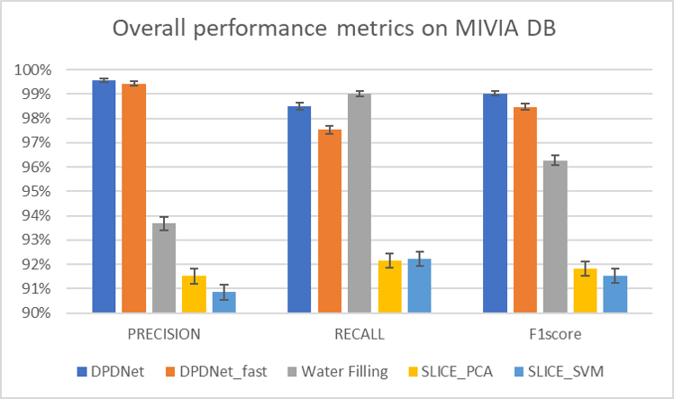
(a) Performance metrics.

.

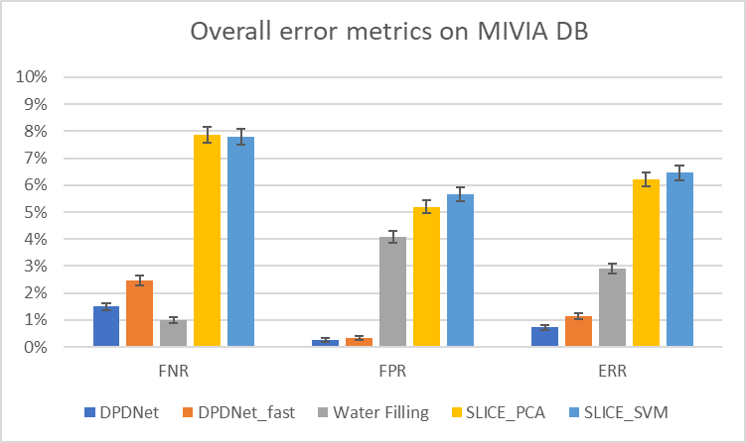
(b) Error metrics.

.

Figure 7: Overall performance and error metrics for the MIVIA dataset.

Table 14 shows the final aggregated results of the evaluated algorithms on the ZHAN2012 dataset, and in Figures 8(a) and 8(b) we show the graphical comparison among the different strategies, where it is again clear how our proposals clearly outperform the other algorithms, with statistically significant improvements.

Table 14: Results for the Zhang2012 dataset. All values in $\%$.

DB	$Precision$	$Recall$	$F_{1}score$	$FNR$	$FPR$	$ERR$
DPDnet	$98.46$	222$\mathbf{99.79}$	$99.12\pm 0.25$	222$\mathbf{0.21}$	$6.87$	$1.44\pm 0.32$
DPDnetfast	222$\mathbf{99.44}$	$99.19$	222$\mathbf{99.31}\pm 0.22$	$0.81$	222$\mathbf{2.47}$	222$\mathbf{1.12\pm 0.28}$
WaterFilling	$95.70$	$98.79$	$97.22\pm 0.44$	$1.21$	$19.71$	$4.61\pm 0.57$
SLICEPCA*	$94.35$	$98.16$	$96.22\pm 0.52$	$1.84$	$25.69$	$6.28\pm 0.66$
SLICESVM*	$77.50$	$79.44$	$78.46\pm 1.10$	$20.56$	$110.57$	$36.09\pm 1.29$
MexicanHat	$36.56$	$23.68$	$28.74\pm 1.22$	$76.32$	$182.85$	$95.87\pm 0.54$

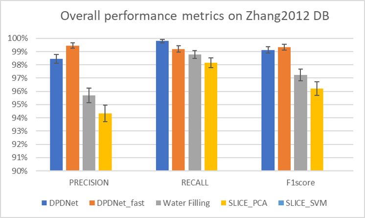
(a) Performance metrics.

.

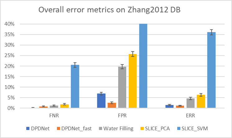
(b) Error metrics.

.

Figure 8: Overall performance and error metrics for the Zhang2012 dataset.

3.5 Computational Performance Evaluation

Regarding the computational demands, Table 15 shows the performance of the evaluated algorithms measured in average frames per second (we have explicitly removed results for MexicanHat due to its bad performance and its bad results in computational behavior according to the results shown in [26]).

All the experiments shown were run in a standard PC, with an Intel I7-6700 at 3.4GHz and 32Gb RAM. The GPU used was an NVIDIA GTX 1080 Ti. The evaluation was run on samples from the GOTPD1+ dataset.

In the case of the DPDnet and DPDnet_fast we also show CPU results.

	DPDnet	DPDnetfast	WaterFilling	SLICEPCA	SLICESVM
FPS (CPU)	$2.7$	$9.8$	$16.6$	$312.0$	$406.0$
FPS (GPU)	$65.4$	$116.9$	N/A	N/A	N/A

Table 15: Timing Results, measured as average frames per second (FPS).

As it can be clearly seen, the computational performance of the DNN based strategies running on a generic CPU is well behind that obtained by the WaterFilling and SLICE approaches, although the DPDnet_fast could run at a reasonable rate of 10 FPS. The performance of the SLICE algorithms is much better than the one reported in [26] as the CPU we use is significantly better. When the GPU enters the competition, the results for DPDnet and DPDnet_fast are, as expected, much better than those for WaterFilling, but still behind SLICE_SVM and SLICE_PCA. However both DNN-based strategies are well above the requirements demanded for real time operation. Taking into account that these approaches significantly outperform the other methods, there is still room for further reduction in the network complexity.

In what respect to the effect of the scene complexity on the computational performance of the algorithms, [26] already showed that the SLICE_PCA algorithm was affected by the number of persons in the scene (this was due to the fact that the ROI estimation and the feature extraction modules, which demands that are proportional to the number of people, had a big impact in the processing time). On the other hand, the DPDnet, DPDnet_fast, and WaterFilling algorithms do not exhibit such a scene complexity dependence.Table 16 shows the FPS performance for these algorithms evaluated on sequences with one, two, and more than two people. It can be seen that there is no direct impact of the number of persons on the results for DPDnet, DPDnet_fast, and WaterFilling. For the SLICE_PCA and SLICE_SVM approaches, the relative decrease in computational performance between the FPS for the single and more than two people cases is of $65.3\%$ and $58.4\%$, respectively.

	DPDnet (GPU)	DPDnetfast (GPU)	WaterFilling	SLICEPCA	SLICESVM
Single person	$66.9$	$111.5$	$16.6$	$572.0$	$682.0$
Two people	$60.9$	$124.0$	$16.8$	$391.8$	$498.8$
More than two people	$65.5$	$117.5$	$16.5$	$198.7$	$283.4$

Table 16: Average timing results for the WaterFilling, DPDnet and DPDnet_fast algorithms for sequences with varying number of users (FPS).

4 Conclusions

In this work we propose two specific neural networks (DPDnet and DPDnet_fast) that detect multiple people from depth data captured by an overhead ToF sensor. We evaluate and compare our method with other recent state-of-the-art methods using three different depth image datasets and following a rigorous experimental procedure. We took into account that the training and testing subsets were fully independent, and that the scenes were as realistic as possible, that is, that they contained people of different heights, with different hairstyles, wearing different,talking on a mobile phone, and that there were objects such as different types of chairs.

Our proposal outperforms the other methods in all datasets even when the number of people is high and they are very close to each other. Additionally, there was no need to retrain nor fine-tune the network to the different datasets used.

Comparing the two proposed method, DPDnet_fast is $38\%$ faster than DPDnet at the cost of $0.1\%$ loss decrement in accuracy. Future works include adaptation of our approach to work with non-overhead depth sensors and the use of other network topologies to improve accuracy and efficiency.

References

- [1] A. F. Agarap. Deep learning using rectified linear units (relu). arXiv preprint arXiv:1803.08375, 2018.
- [2] M. Andriluka, S. Roth, and B. Schiele. People-tracking-by-detection and people-detection-by-tracking. In 2008 IEEE Conference on Computer Vision and Pattern Recognition, pages 1–8, June 2008.
- [3] B. Antic, D. Letic, D. Culibrk, and V. Crnojevic. K-means based segmentation for real-time zenithal people counting. In Proceedings of the 16th IEEE International Conference on Image Processing, ICIP’09, pages 2537–2540, Piscataway, NJ, USA, 2009. IEEE Press.
- [4] V. Badrinarayanan, A. Kendall, and R. Cipolla. Segnet: A deep convolutional encoder-decoder architecture for image segmentation. CoRR, abs/1511.00561, 2015.
- [5] A. Bevilacqua, L. Di Stefano, and P. Azzari. People tracking using a time-of-flight depth sensor. In Video and Signal Based Surveillance, 2006. AVSS ’06. IEEE International Conference on, pages 89–89, Nov 2006.
- [6] A. Brunetti, D. Buongiorno, G. F. Trotta, and V. Bevilacqua. Computer vision and deep learning techniques for pedestrian detection and tracking: A survey. Neurocomputing, 300:17 – 33, 2018.
- [7] Z. Cai, Z. L. Yu, H. Liu, and K. Zhang. Counting people in crowded scenes by video analyzing. In Industrial Electronics and Applications (ICIEA), 2014 IEEE 9th Conference on, pages 1841–1845, June 2014.
- [8] Y. Cao, C. Shen, and H. T. Shen. Exploiting depth from single monocular images for object detection and semantic segmentation. IEEE Transactions on Image Processing, 26(2):836–846, 2017.
- [9] A. Chan, Z.-S. Liang, and N. Vasconcelos. Privacy preserving crowd monitoring: Counting people without people models or tracking. In Computer Vision and Pattern Recognition, 2008. CVPR 2008. IEEE Conference on, pages 1–7, June 2008.
- [10] T.-Y. Chen, C.-H. Chen, D.-J. Wang, and Y.-L. Kuo. A people counting system based on face-detection. In Genetic and Evolutionary Computing (ICGEC), 2010 Fourth International Conference on, pages 699–702, Dec 2010.
- [11] F. Chollet. Xception: Deep learning with depthwise separable convolutions. CoRR, abs/1610.02357, 2016.
- [12] B.-K. Dan, Y.-S. Kim, Suryanto, J.-Y. Jung, and S.-J. Ko. Robust people counting system based on sensor fusion. Consumer Electronics, IEEE Transactions on, 58(3):1013–1021, August 2012.
- [13] L. Del Pizzo, P. Foggia, A. Greco, G. Percannella, and M. Vento. Counting people by rgb or depth overhead cameras. Pattern Recognition Letters, 2016.
- [14] X. Du, M. El-Khamy, J. Lee, and L. Davis. Fused dnn: A deep neural network fusion approach to fast and robust pedestrian detection. In Applications of Computer Vision (WACV), 2017 IEEE Winter Conference on, pages 953–961. IEEE, 2017.
- [15] A. Fernandez-Rincon, D. Fuentes-Jimenez, C. Losada, M. Marron, C. A. Luna, J. Macias-Guarasa, and M. Mazo. Robust people detection and tracking from an overhead time-of-flight camera. In 12th International Conference on Computer Vision Theory and Applications., volume 4, pages 556–564, Porto, Portugal, 03/2017 2017.
- [16] F. Galčík and R. Gargalík. Real-time depth map based people counting. In International Conference on Advanced Concepts for Intelligent Vision Systems, pages 330–341. Springer, 2013.
- [17] C. Gao, P. Li, Y. Zhang, J. Liu, and L. Wang. People counting based on head detection combining adaboost and cnn in crowded surveillance environment. Neurocomputing, 208:108–116, 2016.
- [18] K. He, X. Zhang, S. Ren, and J. Sun. Deep residual learning for image recognition. In Proceedings of the IEEE conference on computer vision and pattern recognition, pages 770–778, 2016.
- [19] S. Hoo-Chang, H. R. Roth, M. Gao, L. Lu, Z. Xu, I. Nogues, J. Yao, D. Mollura, and R. M. Summers. Deep convolutional neural networks for computer-aided detection: Cnn architectures, dataset characteristics and transfer learning. IEEE transactions on medical imaging, 35(5):1285, 2016.
- [20] C. Y. Jeong, S. Choi, and S. W. Han. A method for counting moving and stationary people by interest point classification. In Image Processing (ICIP), 2013 20th IEEE International Conference on, pages 4545–4548, Sept 2013.
- [21] L. Jia and R. Radke. Using time-of-flight measurements for privacy-preserving tracking in a smart room. Industrial Informatics, IEEE Transactions on, 10(1):689–696, Feb 2014.
- [22] D. P. Kingma and J. Ba. Adam: A method for stochastic optimization. arXiv preprint arXiv:1412.6980, 2014.
- [23] A. Krizhevsky, I. Sutskever, and G. E. Hinton. Imagenet classification with deep convolutional neural networks. In Advances in neural information processing systems, pages 1097–1105, 2012.
- [24] M. R. Lab. The MIVIA People Counting Dataset. Available online, 2016. (accessed July 2018).
- [25] J. Liu, Y. Liu, G. Zhang, P. Zhu, and Y. Q. Chen. Detecting and tracking people in real time with rgb-d camera. Pattern Recognition Letters, 53:16 – 23, 2015.
- [26] C. A. Luna, C. Losada-Gutierrez, D. Fuentes-Jimenez, A. Fernandez-Rincon, M. Mazo, and J. Macias-Guarasa. Robust people detection using depth information from an overhead time-of-flight camera. Expert Systems with Applications, 71:240–256, 2017.
- [27] J. Macias-Guarasa, C. Losada-Gutierrez, D. Fuentes-Jimenez, R. Fernandez, C. A. Luna, A. Fernandez-Rincon, and M. Mazo. The GEINTRA Overhead ToF People Detection (GOTPD1) database. Available online, 2016. (accessed June 2019).
- [28] M. Munaro, C. Lewis, D. Chambers, P. Hvass, and E. Menegatti. Rgb-d human detection and tracking for industrial environments. In E. Menegatti, N. Michael, K. Berns, and H. Yamaguchi, editors, Intelligent Autonomous Systems 13, pages 1655–1668, Cham, 2016. Springer International Publishing.
- [29] D. T. Nguyen, W. Li, and P. O. Ogunbona. Human detection from images and videos: A survey. Pattern Recognition, 51:148 – 175, 2016.
- [30] W. Ouyang and X. Wang. Joint deep learning for pedestrian detection. In Proceedings of the IEEE International Conference on Computer Vision, pages 2056–2063, 2013.
- [31] D. Ramanan, D. A. Forsyth, and A. Zisserman. Tracking People by Learning Their Appearance. Pattern Analysis and Machine Intelligence, IEEE Transactions on, 29(1):65–81, Nov. 2006.
- [32] M. Rauter. Reliable human detection and tracking in top-view depth images. In Proceedings of the IEEE Conference on Computer Vision and Pattern Recognition Workshops, pages 529–534, 2013.
- [33] J. Redmon, S. Divvala, R. Girshick, and A. Farhadi. You only look once: Unified, real-time object detection. In Proceedings of the IEEE conference on computer vision and pattern recognition, pages 779–788, 2016.
- [34] X. Ren, S. Du, and Y. Zheng. Parallel rcnn: A deep learning method for people detection using rgb-d images. In Image and Signal Processing, BioMedical Engineering and Informatics (CISP-BMEI), 2017 10th International Congress on, pages 1–6. IEEE, 2017.
- [35] C. Stahlschmidt, A. Gavriilidis, J. Velten, and A. Kummert. People detection and tracking from a top-view position using a time-of-flight camera. In A. Dziech and A. Czyazwski, editors, Multimedia Communications, Services and Security, volume 368 of Communications in Computer and Information Science, pages 213–223. Springer Berlin Heidelberg, 2013.
- [36] C. Stahlschmidt, A. Gavriilidis, J. Velten, and A. Kummert. Applications for a people detection and tracking algorithm using a time-of-flight camera. Multimedia Tools and Applications, pages 1–18, 2014.
- [37] R. Stewart, M. Andriluka, and A. Y. Ng. End-to-end people detection in crowded scenes. In Proceedings of the IEEE conference on computer vision and pattern recognition, pages 2325–2333, 2016.
- [38] P. Vera, S. Monjaraz, and J. Salas. Counting pedestrians with a zenithal arrangement of depth cameras. Machine Vision and Applications, 27(2):303–315, 2016.
- [39] C. Wang and Y. Zhao. Multi-layer proposal network for people counting in crowded scene. In Intelligent Computation Technology and Automation (ICICTA), 2017 10th International Conference on, pages 148–151. IEEE, 2017.
- [40] Z. YunFei, X. Zhang, W. Feng, T. Cao, M. Sun, and W. Xiaobing. Detection of people with camouflage pattern via dense deconvolution network. IEEE Signal Processing Letters, 2018.
- [41] S. Zhang, R. Benenson, M. Omran, J. Hosang, and B. Schiele. How far are we from solving pedestrian detection? In Proceedings of the IEEE Conference on Computer Vision and Pattern Recognition, pages 1259–1267, 2016.
- [42] S. Zhang, R. Benenson, M. Omran, J. Hosang, and B. Schiele. Towards reaching human performance in pedestrian detection. IEEE Transactions on Pattern Analysis and Machine Intelligence, 40(4):973–986, April 2018.
- [43] X. Zhang, J. Yan, S. Feng, Z. Lei, D. Yi, and S. Li. Water filling: Unsupervised people counting via vertical Kinect sensor. In Advanced Video and Signal-Based Surveillance (AVSS), 2012 IEEE Ninth International Conference on, pages 215–220, Sept 2012.
- [44] J. Zhao, G. Zhang, L. Tian, and Y. Q. Chen. Real-time human detection with depth camera via a physical radius-depth detector and a cnn descriptor. In 2017 IEEE International Conference on Multimedia and Expo (ICME), pages 1536–1541, July 2017.
- [45] K. Zhou, A. Paiement, and M. Mirmehdi. Detecting humans in rgb-d data with cnns. In Machine Vision Applications (MVA), 2017 Fifteenth IAPR International Conference on, pages 306–309. IEEE, 2017.
- [46] L. Zhu and K.-H. Wong. Human tracking and counting using the kinect range sensor based on adaboost and kalman filter. In International Symposium on Visual Computing, pages 582–591. Springer, 2013.