[2006.01045] 1 Reviewer #1

Response to Reviewers Comments

The authors are grateful to the editors and two anonymous reviewers for their suggestions to improve the manuscript. All comments of the reviewers have been carefully considered.

1 Reviewer #1

1. In Section 4, the diagram of HCG architecture has a certain degree of repetition, and the information expression is not clear enough.

Response and Revision: Thank you for your kind comments. We have removed the repetition in Section 4. To make the expression clear, we have redrawn the figures and reorganized the contents in Section 4. The modified contents in Section 4 are presented in the following.

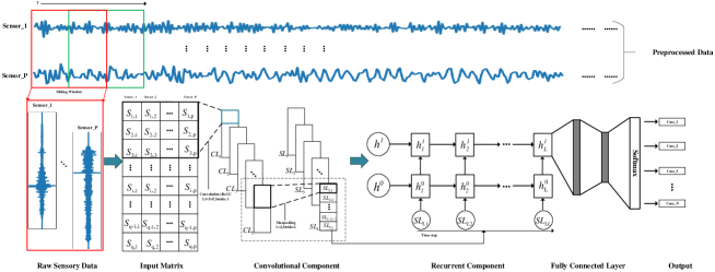
4.1 Architecture of HCG

The architecture of HCG is shown in Fig 1. Our hierarchical model has a low-level convolutional component that learns from interactions among sensors and the short-term temporal dependencies, and a high-level recurrent component that handles information across long-term temporal dependencies.

The inputs of HCG are the time-series data of multiple sensors, while the outputs are the generated predictions of the structures. First, the raw sensory time-series data is modeled into the input matrix as discussed in Section 3.2 and is fed into our proposed convolutional component. Second, our proposed convolutional component is leveraged to learn the spatial and short-term temporal features. Third, the outputs of the convolutional component is fed into the recurrent component to learn the long-term temporal dependencies. Finally, a softmax layer is connected with the latent feature vectors generated by the recurrent component to predict the damage state of the structure.

Refer to caption — Figure 1: Architecture of our proposed HCG.

4.2 Convolutional Component

As discussed in Section 3.3, it is crucial to model both the spatial and temporal dependencies in the sensory signals. Convolutional neural network (CNN) is powerful in capturing the spatial correlations and repeating patterns and has been widely used in image classification, object tracking and video processing [krizhevsky2012imagenet, simonyan2014very], etc.

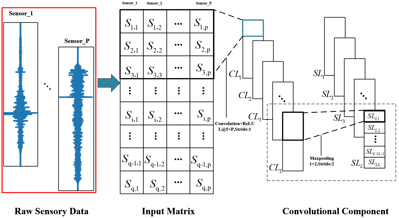
A typical convolution layer contains several convolutional filters. Given the input matrix $\boldsymbol{X}$ defined in Section 3.2, we use these filters to learn the spatial correlations between sensors and the short-term temporal patterns. We let the width of the kernels be the same as the number of sensors so that the kernels are able to capture the spatial correlations among all the sensors. The length of the kernels is relatively short for capturing the short-term temporal patterns. Then, the convolution operation can handle one dimension among the time data as illustrated in Fig. 2. The convolution component finally outputs a corresponding sequence where each element is a latent vector and represents the captured patterns at that moment. Zero-padding is used to ensure the length of the inputs and outputs the same.

Formally, the convolutional layer can be formulated as:

F(\boldsymbol{x}_{t})=(\boldsymbol{X}*\boldsymbol{f})(t)=\sum_{i=0}^{k-1}\boldsymbol{f}_{j}\cdot\boldsymbol{x}_{t-j},\boldsymbol{x}_{\leq 0}\coloneqq 0,

(1)

\boldsymbol{O}=\{F(\boldsymbol{x}_{1}),F(\boldsymbol{x}_{2}),...,F(\boldsymbol{x}_{T})\},

(2)

{\boldsymbol{Y}}=RELU(\boldsymbol{O}),

(3)

where $\boldsymbol{x}_{t}\in\mathbb{R}^{N}$ denotes the values of all the sensors at times $t$ , $\boldsymbol{f}\in\mathbb{R}^{N\times k}$ denotes a convolution kernel with size $k$ and the $RELU$ function $RELU(x)=max(0,x)$ is the activation function, ${\boldsymbol{Y}}=\{\boldsymbol{y}_{1},\boldsymbol{y}_{2},...,\boldsymbol{y}_{T}\}$ denotes the output sequence of our convolutional component. Each element $\boldsymbol{y}_{t}\in\mathbb{R}^{d}$ , where $d$ is the number of the kernels, denotes the latent representation of the spatial and short-term features at time $t$ .

4.3 Recurrent Component

Recurrent neural networks (RNNs) [rumelhart1988learning] have recently shown promising results in many machine learning tasks, especially when input and/or output are a sequence of variables. GRU is a simple and yet powerful variant of RNNs for time series prediction due to the gated mechanism [chung2014empirical, cho2014properties]. GRUs are carefully designed to memorize historical information and fuse current states, new inputs and historical information together in a recurrently gated way.

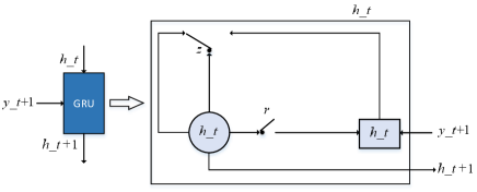
The outputs generated by the convolutional components are fed into the GRU to extract the long-term temporal dependencies. The computing process of the GRU unit at time $t+1$ can be shown in Figure 3 and formulated in Equ. 4:

	$\displaystyle r_{t+1}=\sigma(\Theta_{r}[y_{t+1},h_{t}]+b_{r}),$		(4)
	$\displaystyle u_{t+1}=\sigma(\Theta_{u}[y_{t+1},h_{t}]+b_{u}),$
	$\displaystyle c_{t+1}=tanh(\Theta_{c}[y_{t+1},(r_{t+1}\odot h_{t})]+b_{c}),$
	$\displaystyle h_{t+1}=u_{t+1}\odot h_{t}+(1-u_{t+1})\odot c_{t+1},$

where $h_{t}$ is the hidden state of a GRU generated at the iteration step $t$ and is the original hidden states for the iteration step $t+1$ , $y_{t+1}$ is the hidden features generated by the convolutional component, $h_{t+1}$ is the generated hidden state of a GRU, $r_{t+1}$ and $u_{t+1}$ are the reset gate and update gate at the time $t+1$ , respectively, $\Theta_{r},\Theta_{u}$ and $\Theta_{c}$ are the learned parameters of filters, and $\odot$ is the element-wise multiplication of tensors.

By recurrently connecting the GRU cells, our recurrent component can process complex sequence data. Then, we use the hidden state at the last timestamp of the top-layer GRU to predict the damage category. We use a fully connected and a softmax layer to generate the final output of HCG. Formally, the predicted category $D$ is formulated as:

\boldsymbol{y}^{f}=(\boldsymbol{h}_{T}^{N_{l}})^{\mathsf{T}}\boldsymbol{W}+\boldsymbol{b},

(5)

\displaystyle d_{i}=Softmax(\boldsymbol{y}^{f})_{i}=\frac{{{e^{{y^{f}_{i}}}}}}{{\sum\nolimits_{j=1}^{N_{c}}{{e^{{y^{f}_{j}}}}}}},

(6)

D=\arg\max_{i\in 1,...,N_{c}}d_{i},

(7)

where $\boldsymbol{y}^{f}\in\mathbb{R}^{N_{c}}$ is the output of the fully connected layer, $N_{l}$ is the number of GRU layers, $N_{c}$ denotes the number of categories, $\boldsymbol{W}$ and $\boldsymbol{b}$ are trainable parameters, $\boldsymbol{h}^{i}_{t}$ denotes the hidden state of the $i$ -th GRU layer at timestamp $t$ , and $d_{i}=P(D=i|\boldsymbol{X})$ is the predicted probability for the $i$ -th category.

4.4 Loss Function

In the training process, we adopt mean squared error (L2-loss) as the objective function, the corresponding optimization objective is formulated as:

\min_{\boldsymbol{\Theta}}\sum_{j=0}^{M}\sum_{i=0}^{G}(\boldsymbol{d}_{t,i}^{j}-\hat{\boldsymbol{d}}_{t,i}^{j})^{2},

(8)

where $\boldsymbol{\Theta}$ denotes the parameters set of our model, and $G$ is the number of training samples, $\boldsymbol{d}$ is the ground truth of the damage state, $\hat{\boldsymbol{d}}$ is the predicted class of our model. ，

2. In Section V Performance Evaluation and Discussion, the experimental results of the proposed HCG method are compared with the classical DNN, CNN, LSTM, GRU methods. According to the experimental results, it is concluded that the HCG method has comparative advantages in terms of computing efficiency and memory usage. This conclusion is based on assumptions about specific structures and parameters, not the optimal structure and parameters of the model. Therefore, the conclusion of this paper needs more detailed experimental results support.

Response and Revision: Thanks a lot for your comments. To verify that our proposed HCG method has comparative advantages in terms of performance, computing efficiency and memory usage. We vary different layers and different parameters for DNN, CNN, LSTM, GRU and HCG to show the performance. The performance shows that our proposed HCG outperforms other method under different parameters. The added contents in Section 5 are listed as follows.

Section 5.4 Performance Analysis of Hyper-parameters in the TCRF Bridge Dataset

In order to further demonstrate the advantages of the proposed HCG method rather than a set of a selected hyper-parameters, we compared and analyzed the performance of different hyper-parameters, including network structure and number of neurons, of DNN, CNN, LSTM, RNN, and HCG for the TCRF Bridge dataset.

We first conduct a set of experiments to study the effectiveness of the network structure, we adopted the network structure shown in table 1 to measure and compare the performance of the DNN, CNN, LSTM, RNN, and HCG model. In the table, $2$ -layer, $3$ -layer, $4$ -layer, $5$ -layer mean the number of neural network layers for the models. The number of neurons are the same for all the models for fair comparison.

Table 1: Results on different layers for the TCRF Bridge dataset

Model	2-layer	3-layer	4-layer	5-layer
DNN	0.925±0.001	0.929±0.002	0.934±0.002	0.933±0.002
CNN	0.928±0.002	0.932±0.002	0.934±0.002	0.931±0.001
LSTM	0.863±0.002	0.909±0.001	0.902±0.003	0.882±0.003
GRU	0.892±0.002	0.907±0.003	0.900±0.003	0.887±0.002
HCG	0.945±0.002	0.946±0.002	0.948±0.002	0.947±0.001

We then conduct another set of experiments to study the effectiveness of the number of neurons, we adopt the $4$ -layer set because of the $4$ -layer set achieves higher accuracy than others. We chose different number of neurons for all the models. The results are listed in Table 2. In the table, ${[}40,70,32,32{]}$ means $40$ , $70$ , $32$ , and $32$ neurons for the $4$ layers respectively.

Table 2: Results on different numbers of neurons for the TCRF Bridge dataset

Model	[40, 70, 32, 32]	[40, 70, 32, 64]	[40, 70, 64, 64]	[40, 70, 64, 100]
DNN	0.924±0.003	0.928±0.001	0.933±0.0.3	0.932±0.001
CNN	0.927±0.002	0.932±0.004	0.935±0.002	0.933±0.002
LSTM	0.864±0.002	0.907±0.002	0.904±0.003	0.881±0.002
GRU	0.892±0.003	0.905±0.003	0.902±0.003	0.888±0.001
HCG	0.9469±0.003	0.944±0.002	0.946±0.003	0.949±0.002

From both the tables, it can be concluded that HCG has higher accuracy in different hyper-parameter sets compared with neural network model. HCG model learns from interactions among sensors and the short-term temporal dependencies, and a high-level component that handles information across long-term temporal dependencies, which has excellent advantages.

Section 5.6 Performance Analysis of Hyper-parameters in the IASC-ASCE Benchmark Dataset

Like in TCRF Bridge Dataset, in order to further demonstrate the advantages of the proposed HCG method rather than a set of a selected hyper-parameters, we compared and analyzed the performance of different hyper-parameters, including network structure and number of neurons, of DNN, CNN, LSTM, RNN, and HCG for the IASC-ASCE Benchmark Dataset.

We first conduct a set of experiments to study the effectiveness of the network structure, we adopted the network structure shown in table 3 to measure and compare the performance of the DNN, CNN, LSTM, RNN, and HCG model. In the table, $2$ -layer, $3$ -layer, $4$ -layer, $5$ -layer mean the number of neural network layers for the models. The number of neurons are the same for all the models for fair comparison.

Table 3: Results on different layers for the IASC-ASCE Benchmark Dataset

Model	2-layer	3-layer	4-layer	5-layer
DNN	0.836±0.004	0.837±0.001	0.839±0.002	0.831±0.002
CNN	0.832±0.005	0.836±0.002	0.840±0.003	0.836±0.001
LSTM	0.835±0.002	0.833±0.003	0.831±0.002	0.832±0.002
GRU	0.837±0.002	0.834±0.001	0.839±0.002	0.833±0.004
HCG	0.841±0.002	0.841±0.002	0.842±0.003	0.842±0.003

Table 4: Results on different numbers of neurons for the IASC-ASCE Benchmark Dataset

Model	[32, 32, 32, 64]	[32, 32, 64, 64]	[32, 64, 64, 64]	[64, 64, 64, 64]
DNN	0.835±0.002	0.836±0.003	0.839±0.002	0.831±0.002
CNN	0.834±0.002	0.834±0.002	0.840±0.001	0.831±0.002
LSTM	0.833±0.004	0.834±0.001	0.835±0.002	0.834±0.003
GRU	0.839±0.003	0.833±0.002	0.839±0.002	0.832±0.004
HCG	0.841±0.002	0.843±0.002	0.842±0.002	0.843±0.002

From both the tables, it can be concluded that HCG has higher accuracy in different hyper-parameter sets compared with neural network models.

3. In Section V Performance Evaluation and Discussion, the experimental result curve is not standardized. For example, Fig. 8 has no abscissas and units. The coordinate font sizes of Fig. 8, 10, and 12 are too small.

Response and Revision: Thanks a lot for your comments. We add abscissas of Fig. 8 and enlarge the font sizes of Fig. 8, 10, and 12. The modified contents in Section 5 are listed as follows.

5.1.1. TCRF Bridge Dataset

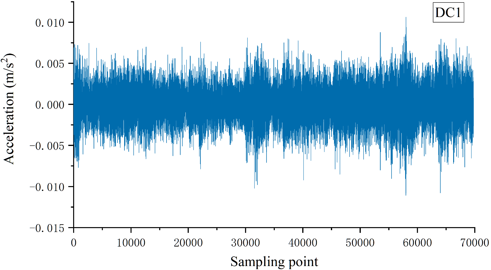
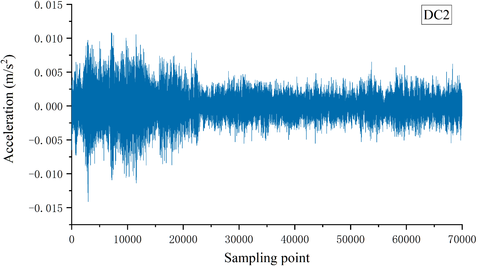
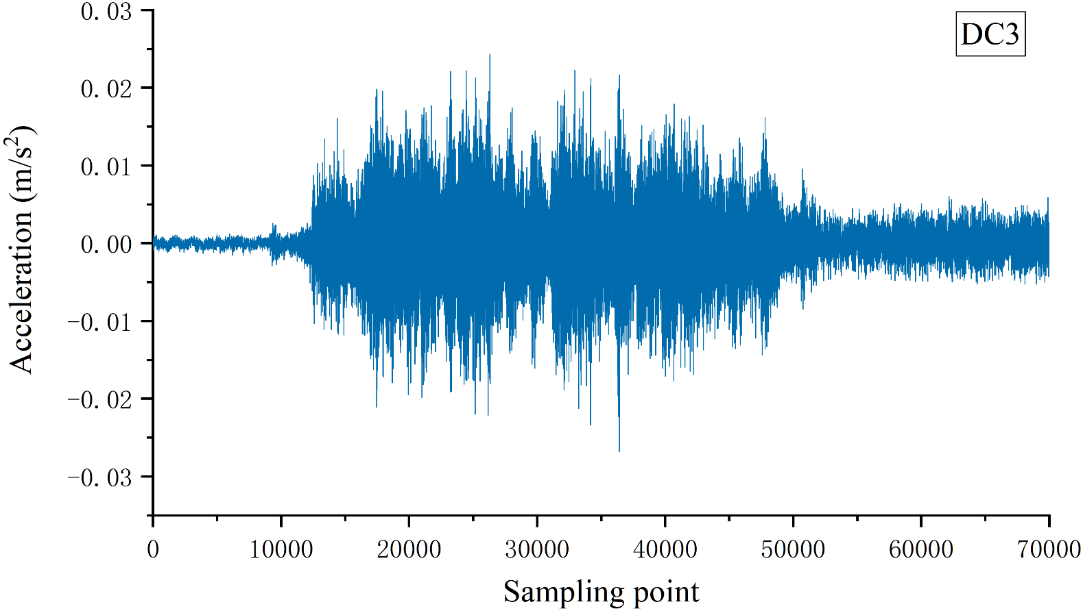
When a car passed through the bridge deck, the acceleration signals of each sensor were collected with the sampling frequency of $8$ khz. The signals were quite different for different damage states. For example, in the case of different structural damage, the curve of acceleration at the second measuring point is shown in Fig. 4. The figure shows that the sensory data keep floating around zero, which accords with the stable time series. It can be observed that the response data is obviously different for different damage states. The HCG model is used to learn the spatial and temporal features of these sensory data.

5.3. Results of the TCRF Bridge Dataset

Table 9 summarizes the experimental results of our proposed HCG and other baselines on the TCRF Bridge Dataset.The Dataset adopt the standard deviation and then We run all the baselines for $10$ times and report the average results. HCG obtains the better results compared with single CNN and GRU model. It shows the effectiveness of considering both the spatial and temporal dependencies together. HCG also outperforms DNN and LSTM based models. Overall, our proposed HCG outperforms other baselines including DNN, CNN, LSTM and GRU on all the evaluation metrics.

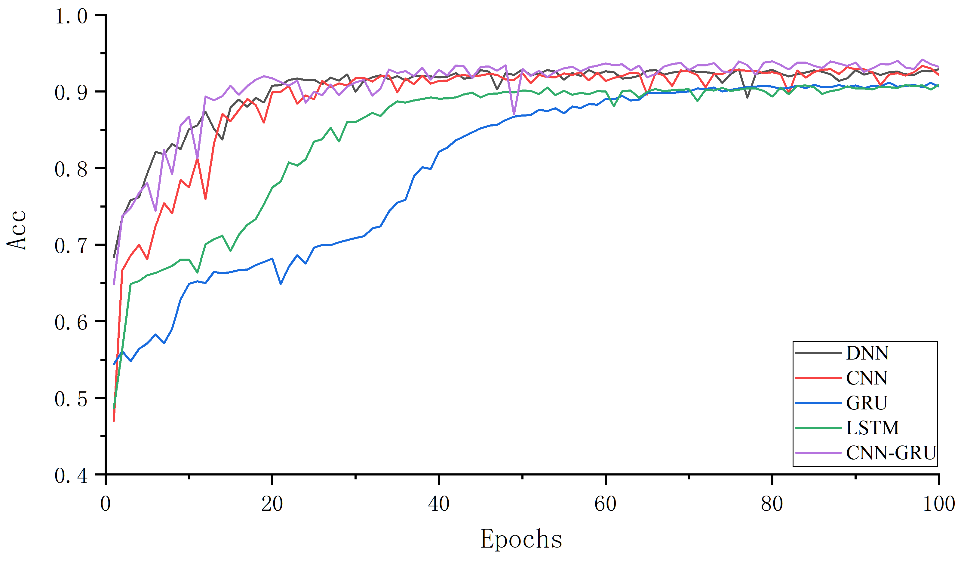
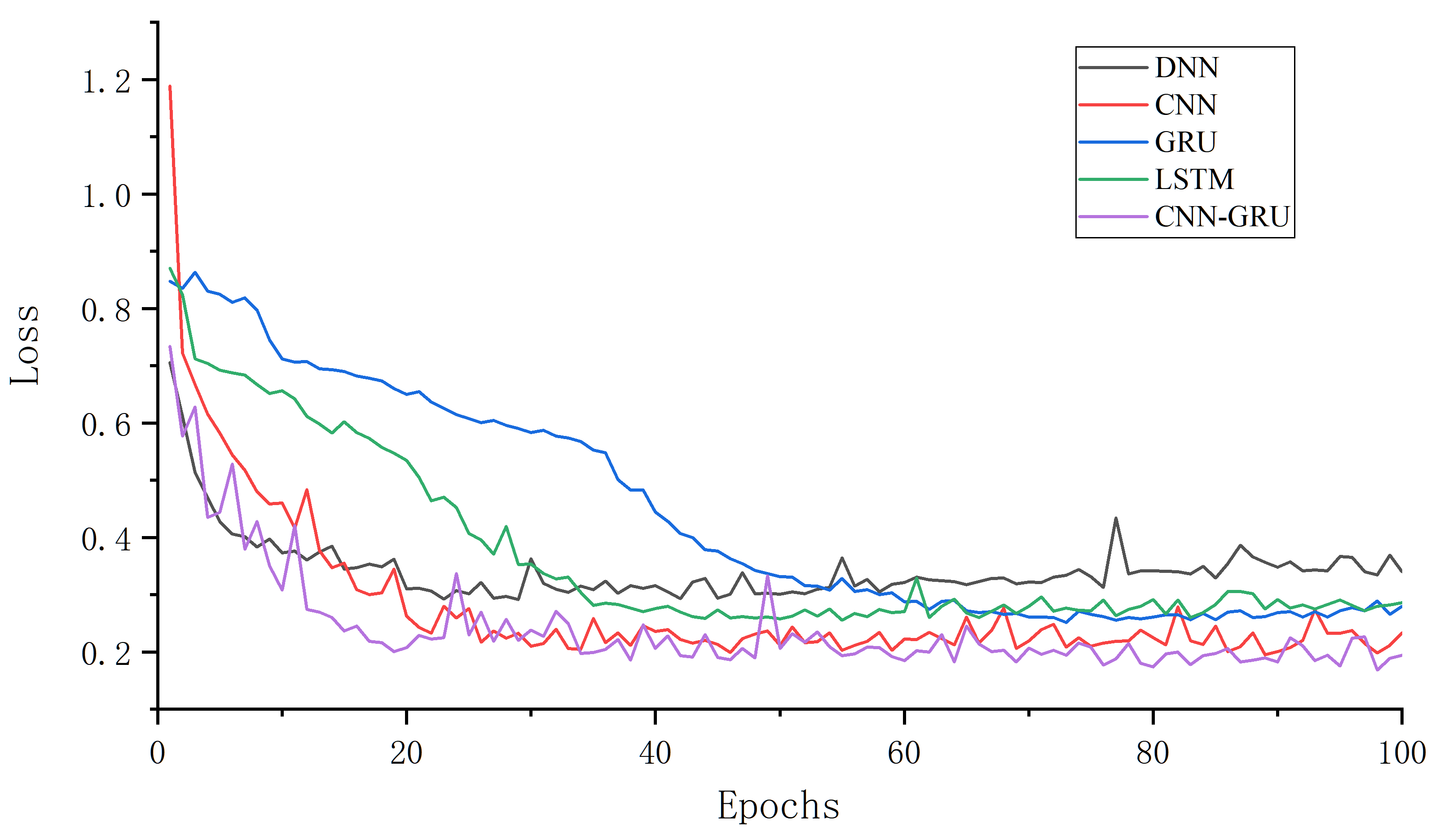
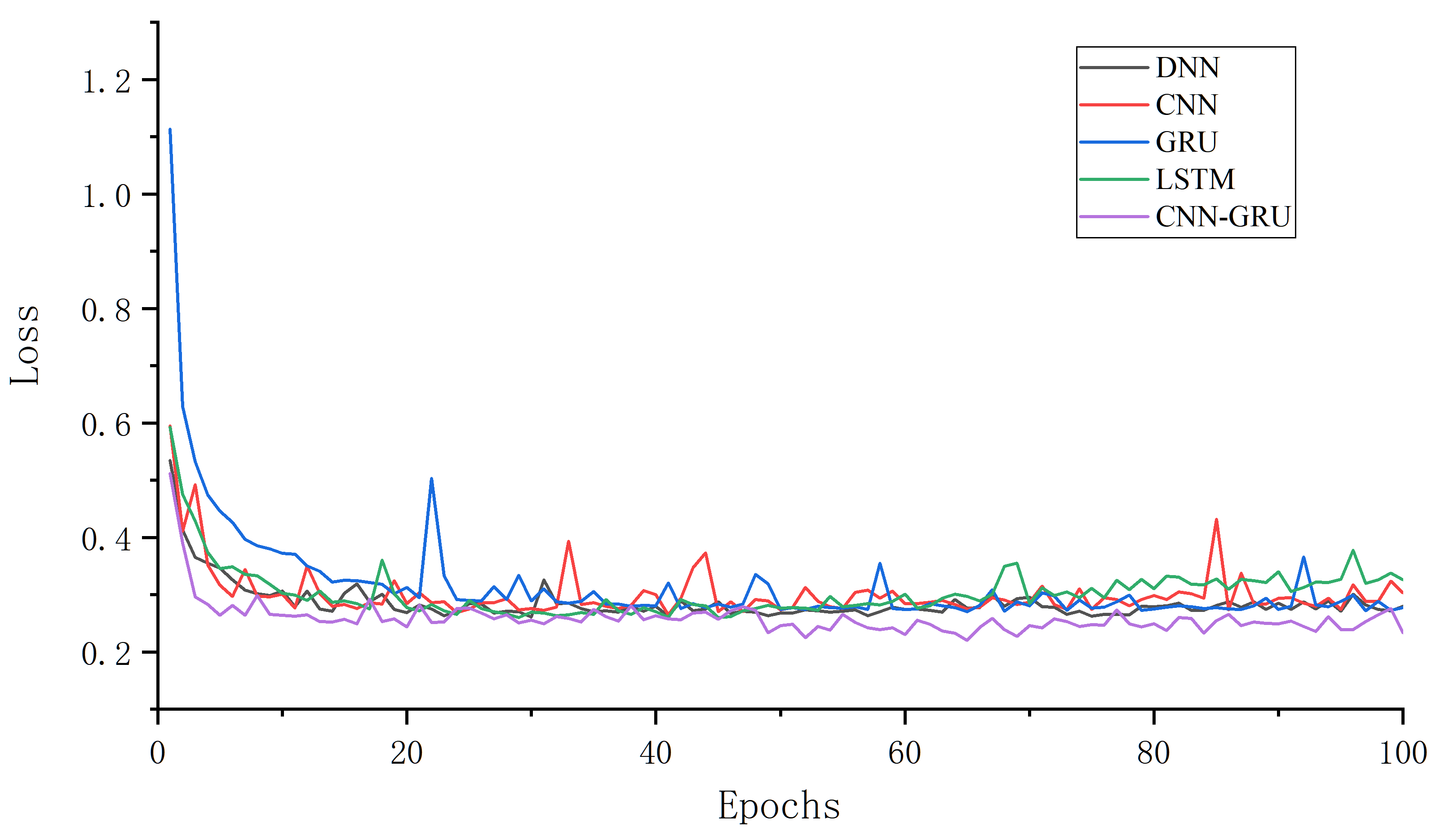
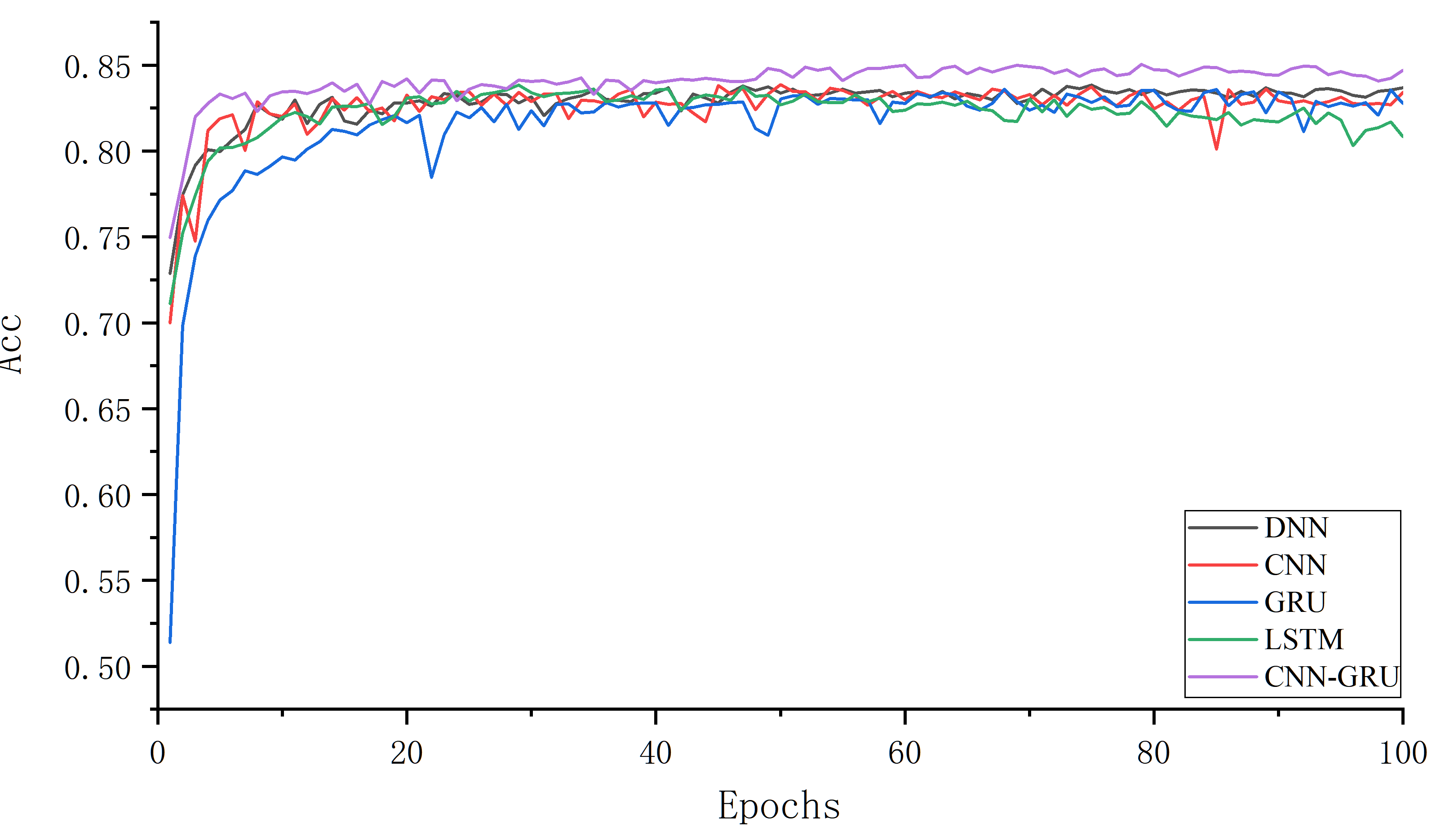
Fig.5 illustrates the loss curve and accuracy curve in the training process for the deep-learning based baselines and our HCG. We can clearly observe that our proposed HCG converges more quickly than other competitors which demonstrate HCG’s priority as HCG can capture both the spatial and temporal dependencies in the sensory data.

5.4. Results of the IASC-ASCE Benchmark Dataset

Table 10 summarize the experimental results on the IASC-ASCE Benchmark Dataset. Fig.6 illustrates the loss curve and accuracy curve in the training process for the deep-learning based baselines and our HCG. Similar with the results in the IASC-ASCE Benchmark Dataset, HCG also shows its priority over other compared baselines.

4. Please check some spelling error and grammatical errors.

Response and Revision: Thanks for pointing them out. We have modified the grammatical issues which you pointed out and have done a thorough review of the entire manuscript, fixing typos and grammar errors.

2 Reviewer #2

1. By fixing the structure of the alternative methods, you are limiting their ability to be optimised for the given data. Are you able to either more clearly justify with evidence why this is a fair comparison.

Section 5.4 Performance Analysis of Hyper-parameters in the TCRF Bridge Dataset

We first conduct a set of experiments to study the effectiveness of the network structure, we adopted the network structure shown in table 5 to measure and compare the performance of the DNN, CNN, LSTM, RNN, and HCG model. In the table, $2$ -layer, $3$ -layer, $4$ -layer, $5$ -layer mean the number of neural network layers for the models. The number of neurons are the same for all the models for fair comparison.

Table 5: Results on different layers for the TCRF Bridge dataset

Model	2-layer	3-layer	4-layer	5-layer
DNN	0.925±0.001	0.929±0.002	0.934±0.002	0.933±0.002
CNN	0.928±0.002	0.932±0.002	0.934±0.002	0.931±0.001
LSTM	0.863±0.002	0.909±0.001	0.902±0.003	0.882±0.003
GRU	0.892±0.002	0.907±0.003	0.900±0.003	0.887±0.002
HCG	0.945±0.002	0.946±0.002	0.948±0.002	0.947±0.001

We then conduct another set of experiments to study the effectiveness of the number of neurons, we adopt the $4$ -layer set because of the $4$ -layer set achieves higher accuracy than others. We chose different number of neurons for all the models. The results are listed in Table 6. In the table, ${[}40,70,32,32{]}$ means $40$ , $70$ , $32$ , and $32$ neurons for the $4$ layers respectively.

Table 6: Results on different numbers of neurons for the TCRF Bridge dataset

Model	[40, 70, 32, 32]	[40, 70, 32, 64]	[40, 70, 64, 64]	[40, 70, 64, 100]
DNN	0.924±0.003	0.928±0.001	0.933±0.0.3	0.932±0.001
CNN	0.927±0.002	0.932±0.004	0.935±0.002	0.933±0.002
LSTM	0.864±0.002	0.907±0.002	0.904±0.003	0.881±0.002
GRU	0.892±0.003	0.905±0.003	0.902±0.003	0.888±0.001
HCG	0.9469±0.003	0.944±0.002	0.946±0.003	0.949±0.002

Section 5.6 Performance Analysis of Hyper-parameters in the IASC-ASCE Benchmark Dataset

We first conduct a set of experiments to study the effectiveness of the network structure, we adopted the network structure shown in table 7 to measure and compare the performance of the DNN, CNN, LSTM, RNN, and HCG model. In the table, $2$ -layer, $3$ -layer, $4$ -layer, $5$ -layer mean the number of neural network layers for the models. The number of neurons are the same for all the models for fair comparison.

Table 7: Results on different layers for the IASC-ASCE Benchmark Dataset

Model	2-layer	3-layer	4-layer	5-layer
DNN	0.836±0.004	0.837±0.001	0.839±0.002	0.831±0.002
CNN	0.832±0.005	0.836±0.002	0.840±0.003	0.836±0.001
LSTM	0.835±0.002	0.833±0.003	0.831±0.002	0.832±0.002
GRU	0.837±0.002	0.834±0.001	0.839±0.002	0.833±0.004
HCG	0.841±0.002	0.841±0.002	0.842±0.003	0.842±0.003

Table 8: Results on different numbers of neurons for the IASC-ASCE Benchmark Dataset

Model	[32, 32, 32, 64]	[32, 32, 64, 64]	[32, 64, 64, 64]	[64, 64, 64, 64]
DNN	0.835±0.002	0.836±0.003	0.839±0.002	0.831±0.002
CNN	0.834±0.002	0.834±0.002	0.840±0.001	0.831±0.002
LSTM	0.833±0.004	0.834±0.001	0.835±0.002	0.834±0.003
GRU	0.839±0.003	0.833±0.002	0.839±0.002	0.832±0.004
HCG	0.841±0.002	0.843±0.002	0.842±0.002	0.843±0.002

From both the tables, it can be concluded that HCG has higher accuracy in different hyper-parameter sets compared with neural network models.

2. In section 5.3, you state that you ”..run the baselines for 10 times and report the average results.” Table 3 and Table 4 present the accuracy, precision, recall and F-1 for the TCRF and IASC-ASCE data sets respectively. Please add the standard deviation of the reported performance vales from the 10 runs for your method and the alternative approaches..

Response and Revision: Thanks for your comments. We have reported the the standard deviation of the performance for the baselines and our proposed HCG. The modified contents in Section 5.3 and 5.4 are listed as follows.

5.3. Results of the TCRF Bridge Dataset

Table 9: Results of the TCRF Bridge Dataset.

Network model	Accuracy	Precision	Recall	F_1
DNN	0.929±0.002	0.918±0.003	0.928±0.003	0.925±0.002
CNN	0.932±0.004	0.913±0.005	0.928±0.004	0.920±0.004
LSTM	0.909±0.002	0.893±0.003	0.908±0.003	0.897±0.003
GRU	0.907±0.003	0.880±0.002	0.923±0.003	0.890±0.002
HCG	0.946±0.003	0.920±0.003	0.945±0.002	0.930±0.002

5.4. Results of the IASC-ASCE Benchmark Dataset

Table 10: Results of the IASC-ASCE Benchmark Dataset.

Network model	Accuracy	Precision	Recall	F1-score
DNN	0.837±0.002	0.837±0.002	0.867±0.001	0.768±0.001
CNN	0.836±0.003	0.836±0.001	0.890±0.003	0.771±0.003
LSTM	0.833±0.002	0.834±0.004	0.887±0.002	0.768±0.003
GRU	0.834±0.002	0.834±0.003	0.881±0.003	0.764±0.002
HCG	0.841±0.002	0.841±0.002	0.909±0.002	0.781±0.001

3. Please check some spelling error and grammatical errors.