Temporal-Differential Learning in Continuous Environments

Abstract

In this paper, a new reinforcement learning (RL) method known as the method of temporal differential is introduced. Compared to the traditional temporal-difference learning method, it plays a crucial role in developing novel RL techniques for continuous environments. In particular, the continuous-time least squares policy evaluation (CT-LSPE) and the continuous-time temporal-differential (CT-TD) learning methods are developed. Both theoretical and empirical evidences are provided to demonstrate the effectiveness of the proposed temporal-differential learning methodology.

Keywords: Reinforcement Learning, Markov Processes, Kernel Methods, Continuous Environment, Policy Evaluation

1 Introduction

Over the past decade, reinforcement learning (RL) has quickly become one of the most prominent technologies in the field of artificial intelligence (AI). The popularity of RL is mainly driven by its recent success in various application fields (Barto et al., 2017; Silver et al., 2017; Wang et al., 2018; Kolm and Ritter, 2019). Despite the rapid growth of RL in recent years, a common feature in most existing RL techniques, or broadly speaking most AI technologies, is that the learning task is performed in discrete learning environments (Russell and Norvig, 2010, Section 2.3.2), that is, either the time space or the state-action space or both are associated with the discrete topology. Although most practical physical environments are continuous in nature, in the sense that both the time space and the state-action spaces are continuous, RL and AI problems in continuous learning environments have rarely been touched upun in the past literature. In fact, the ability of learning in continuous learning environments has long been visioned as an important component of a futuristic AI system (Russell, 1997, Section 7). Admittedly, building AI and RL agents in continuous environments is a challenging task. One challenge is that most processes evolving in continuous environments are described by ordinary differential equations (ODEs), stochastic differential equations (SDEs), or other complex mathematical models. These models are still not fully-understood from the AI and RL perspective. This raises the question on how to develop a generic learning framework applicable to all these models. In addition, the state-action spaces encountered in practical RL problems often exhibit complex shapes and structures. For example, the presence of singularity points in robot workspace (Merlet, 2006) is a notorious issue in robot control and learning. These irregularities create a serious challenge for the convergence and robustness analysis of learning algorithms. Besides its potential value in practical applications, understanding the continuous limits of RL and AI algorithms also provides us a unique insight into the dynamics and theoretical nature of these algorithms. In fact, dynamical systems and differential equation theories have gained great popularity recently in understanding ML, especially neural network (NN) models (E, 2017; Chaudhari et al., 2018; Chen et al., 2018; Ruthotto and Haber, 2020). In addition, the ODE method has already been used in stochastic approximation (Ljung, 1977) to study the convergence of RL algorithms (Kushner and Yin, 2003). Hence, in order to expand the application of RL to a broader range of problems, and to enrich our understanding of RL theory, it is necessary to investigate RL methods in general continuous learning environments.

The purpose of this paper is to extend the classical temporal difference (TD) error (Sutton, 1988) to the setting of continuous environments. To overcome the shortcomings of traditional RL in dealing with problems arising from continuous environments, we will introduce a new concept under the name of temporal-differential error. Similar to the TD in discrete environments, the temporal-differential error plays a key role in developing new RL methods in continuous environments. In particular, we introduce two continuous RL algorithms, namely, the continuous-time least squares policy evaluation (CT-LSPE) (Algorithm 1) and the continuous-time temporal-differential (CT-TD) learning (Algorithm 2). These algorithms are extensions of the LSPE (Nedić and Bertsekas, 2003) and the TD learning (Sutton and Barto, 2018, Chapter 6), respectively, to continuous environments. As a continuous RL methodology, our algorithms also possess several unique features that distinguish them from most traditional RL methods. First, instead of using NN approximation, kernel approximation is used in our design. The linkage between the kernel function and the Hilbert space theory allows our algorithms to achieve convergence over the entire state space. Second, systems and control theory will be applied to show the stability and robustness of the proposed learning algorithms. Finite-time error bounds are also obtained, without assuming the stationarity of the training data as in the past literature (Antos et al., 2008; Munos and Szepesvári, 2008).

2 Related Works

The study on RL in continuous environments can be traced back to the concept of advantage updating (Baird, III, 1993; Harmon et al., 1995). Shortly after Baird’s advantage updating, the continuous-time TD learning and actor-critic algorithms were developed by Doya (1996) and Doya (2000). In addition, Munos (2000) developed a continuous RL technique to solve viscosity solutions in order to tackle the case where the classical optimal solution does not exist. Continuous RL has also been applied in different fields including game theory (Börgers and Sarin, 1997) and neurobiology (Frémaux et al., 2013). A common feature of these early results is that the discrete-time sampling is performed to convert the continuous-time problem into the discrete-time setting. More recently, the research on deep RL opens possibilities for developing practical learning algorithms in continuous state-action spaces (van Hasselt and Wiering, 2007; van Hasselt, 2012; Lillicrap et al., 2016; Duan et al., 2016; Recht, 2019). Indeed, computer experiments from balancing inverted pendulums to learning the locomotion have shown very promising results.

Besides the above collective efforts, a learning-based control design methodology, usually under the name of adaptive (or approximate) dynamic programming (ADP) (Jiang and Jiang, 2012; Vrabie et al., 2013; Bian and Jiang, 2016; Kiumarsi et al., 2018), has been developed to solve optimal control problems for continuous-time dynamical systems. Instead of discretizing a continuous-time system into a discrete-time system, ADP algorithms solve directly the optimal control problem by utilizing the continuous-time data flow generated by dynamical systems. Exploiting explicitly systems and control techniques, the stability and optimality of the controlled system can be guaranteed. Finally, to perform the learning task in more complex environments, robust and decentralized extensions of ADP have also been proposed by Jiang and Jiang (2017); Bian and Jiang (2019).

3 Problem Formulation

Throughout this paper, $\mathbb{R}$ denotes the set of reals. $I$ denotes the identity matrix with appropriate dimension. $|\cdot|$ denotes the Euclidean norm for vectors, or the induced matrix norm for matrices. ${\rm id}$ denotes the identity mapping. Let $(\Omega,\mathcal{F},\mathbb{P})$ be a probability space and $\{x_{t}\}_{t\geq 0}$ be a càdlàg and time-homogeneous strong Markov process with state space $X$. Here $X$ is a locally compact Hausdorff space with a countable base, equipped with the Borel $\sigma$-algebra $\mathcal{B}$. Denote by $\mathbb{E}_{x}$ the expectation conditionally on the initial state $x$ and by $\mathbb{E}_{\mu}$ the expectation with respect to $\mu$. The Hilbert space $L^{2}_{\mu}$ and the norm $\|\cdot\|_{\mu}$ are induced from the inner product $\langle\cdot,\cdot\rangle_{\mu}$ defined via $\langle f,g\rangle_{\mu}=\mathbb{E}_{\mu}\left[fg\right]$ for all $f,g\in L^{2}_{\mu}$. Denote by $\mathcal{A}$ the infinitesimal generator associated with $\{x_{t}\}_{t\geq 0}$. The domain of $\mathcal{A}$ is written as $\mathcal{D}(\mathcal{A})\subseteq L^{2}_{\mu}$. For more details on the notations used in this paper, see Appendix A and references therein.

Our goal in this paper is to estimate the following value function $V^{*}$ that depends on the future path of $\{x_{t}\}_{t\geq 0}$:

$$V^{*}(x) =\mathbb{E}_{x}\left[\int_{0}^{\infty}e^{-\gamma t}r(x_{t})dt\right],\quad\forall x\in X,$$ (1)

where $r\in L^{2}_{\mu}$ is the running-reward/cost function, and $\gamma>0$ is a scalar representing the discounting effect. To be mathematically concrete, we assume $\mathbb{E}_{x}[r(x_{t})]$ is measurable and locally essentially bounded.

To see why the classical discrete-time TD learning is no longer a good choice to solve $V^{*}$ here, we write the discrete-time TD error for the discretized process (with sampling period $\Delta t$) as

$$e^{-\gamma\Delta t}V_{k}(x_{\Delta t})-V_{k}(x)+\int_{0}^{\Delta t}e^{-\gamma s}r(x_{s})ds,\quad\forall x\in X.$$

Obviously, when $\Delta t$ is small, the discounting term $e^{-\gamma\Delta t}$ is close to $1$, resulting in a poor convergence performance (see Tsitsiklis and Van Roy (1997) for convergence analysis). If $\Delta t$ is too large, the updating frequency is reduced, which could also compromise the on-line learning performance. In light of the above difficuities, it is desirable to solve $V^{*}$ without discretizing the performance index and the underlying Markov process in the first place. To proceed, note from Ito (1960, Chapter 1) that $V^{*}$ satisfies the following linear functional equation:

$$0=\mathcal{T}V^{*}+r,$$ (2)

where $\mathcal{T}=\mathcal{A}-\gamma$. The converse statement is also true by Dynkin’s formula (Kushner, 1967a, Chapter 1).

In this paper, we will introduce two on-line learning methods to solve (2).

4 Value Approximation in Continuous Time

In this section, we consider the following approximated equation:

$$\partial_{t}V_{t}=\Pi(\mathcal{T}V_{t}+r),$$ (3)

where $\Pi$ is defined by the following integral equation:

$$\Pi V(x)=\int_{X}V(z)K(z,x)d\mu(z),\quad\forall V\in L^{2}_{\mu},\ x\in X.$$

Here $K$ is a square-integrable continuous symmetric positive-definite kernel. Corresponding to each $K$, we can uniquely define a reproducing kernel Hilbert space (RKHS) $\mathcal{H}\subseteq L^{2}_{\mu}$ (Aronszajn, 1950, Section 2). In addition, $\Pi$ is an orthogonal projection from $L_{\mu}^{2}$ to $\mathcal{H}$ (Aronszajn, 1950, Section 2). To fit into our learning framework, the reproducing kernel $K$ is designed to ensure $\mathcal{H}$ is a subspace of $\mathcal{D}(\mathcal{A})$. This requirement can be satisfied for many practical processes by selecting a sufficiently smooth $K$; see Section 5 for details. Finally, we assume the initial value function $V_{0}\in\mathcal{H}$.

From the perspective of systems and control theory, (3) can be viewed as a reduced-order model (Scarciotti and Astolfi, 2017) of the nominal system

$$\partial_{t}v_{t}=\mathcal{T}v_{t}+r.$$ (4)

As a result, we can rewrite (3) in the form of system (4) with an approximation error $(\Pi-{\rm id})(\mathcal{T}V_{t}+r)$ added to its right-hand side.

The following theorem shows that $V_{t}$ converges into a neighbourhood of $V^{*}$ exponentially.

Theorem 1

$V_{t}$ is well-defined and is exponentially stable (at $V_{\infty}$) in $\mathcal{H}$. In addition,

$$\left\|V_{t}-V^{*}\right\|_{\mu} \leq e^{-\gamma t}\left\|V_{0}-V_{\infty}\right\|_{\mu}+\frac{1}{\gamma}\left\|\mathcal{T}V_{\infty}+r\right\|_{\mu},$$

$$\left\|V_{t}-V^{*}\right\|_{\mu} \leq e^{-\gamma t}\left\|V_{0}-V^{*}\right\|_{\mu}+\frac{1-e^{-\gamma t}}{\gamma}\sup_{s\in[0,t]}\left\|(\Pi-{\rm id})(\mathcal{T}V_{s}+r)\right\|_{\mu}.$$

In particular, $\left\|V_{\infty}-V^{*}\right\|_{\mu}\leq\gamma^{-1}\left\|\mathcal{T}V_{\infty}+r\right\|_{\mu}$.

See Appendix B.1 for the proof of Theorem 1.

The finite-time error bounds in Theorem 1 are composed with two parts. The first part represents the error induced from the initial guess $V_{0}$. The second part is due to the approximation error introduced by the projection $\Pi$. If we can choose $\mathcal{H}$ properly, such that for any $f\in\mathcal{H}$, $\mathcal{A}f\in\mathcal{H}$, then one can show that

$$\left\|V_{t}-V^{*}\right\|_{\mu}\leq e^{-\gamma t}\left\|V_{0}-V^{*}\right\|_{\mu}+\frac{1-e^{-\gamma t}}{\gamma}\|\Pi r-r\|_{\mu}.$$

The above inequality implies that in this case the error bound is purely controlled by the initial guess $V_{0}$ and the “observation error” in the running-reward/cost $r$.

Note that the first error bound in Theorem 1 is tighter for large $t$, and the second error bound is tighter for small $t$. From the perspective of robust control theory, the second error bound quantifies the impact of $(\Pi-{\rm id})(\mathcal{T}V_{t}+r)$ on the approximation error between $V_{t}$ and $V^{*}$. In addition, the discounting factor $\gamma$ is linked to the robustness of (3), in the sense that a larger $\gamma$ results in a smaller error bound and a faster convergence rate.

Finally, it is worth pointing out that the results in Theorem 1 can also be extended to evaluate the ergodic cost (Arapostathis et al., 2012). In this case, there is no discounting term in (1), and we have $\mathcal{T}=\mathcal{A}$ in (2) and (3). Note from Bhattacharya (1982, Proposition 2.2) that as long as $\{x_{t}\}_{t\geq 0}$ is ergodic, $\mathcal{A}$ has a simple zero eigenvalue corresponding to the constant eigenfunction. Hence, by excluding the constant function from $\mathcal{H}$, we can ensure there still exists a $\gamma>0$, such that $\langle V,\Pi\mathcal{T}V\rangle_{\mu}\leq-\gamma\|V\|_{\mu}$. As a result, the two inequalities in Theorem 1 still hold.

5 Model-free On-line Learning

The results presented in the last section provide an efficient way to approximate $V^{*}$ through the linear functional equation (3). Unfortunately, in order to solve (3) directly, we must have access to the knowledge of $\mu$, $\mathcal{A}$, and $r$. This is not an easy task in practice, since $\mu$, $\mathcal{A}$, and $r$ are associated with the mathematical model of the learning environment, which is usually not known.

In this section, we propose two on-line learning algorithms to estimate $V^{*}$ using the data observed directly from the environment. The knowledge of $\mu$, $\mathcal{A}$, and $r$ is not required in our learning algorithm design. Throughout this section, we consider the following realization of $K$:

$$K(z,x)=\phi^{T}(z)\left(\mathbb{E}_{\mu}\left[\phi\phi^{T}\right]\right)^{-1}\phi(x),$$

where $\phi=[\phi_{1}\ \phi_{2}\ \cdots\phi_{N}]^{T}$, and $\{\phi_{j}\}_{j=1}^{N}$ are $N$ independent functions in $\mathcal{D}(\mathcal{A})$. The independence of $\{\phi_{j}\}_{j=1}^{N}$ guarantees the matrix inverse in $K$ is well-defined. Obviously, $K$ satisfies our definition of reproducing kernel in Section 4. In fact, the RKHS $\mathcal{H}$ associated with $K$ is the $N$-dimensional space spanned by $\{\phi_{j}\}_{j=1}^{N}$, and $V_{t}$ in (3) can be parameterized as $V_{t}(x)=\phi^{T}(x)c_{t}$ for some $c_{t}\in\mathbb{R}^{N}$. Directly plugging the definitions of $K$ and $V_{t}$ in (3), we have the following ODE in $c_{t}$:

$$\dot{c}_{t}=\left(\mathbb{E}_{\mu}\left[\phi\phi^{T}\right]\right)^{-1}\left(\mathbb{E}_{\mu}\left[\phi\mathcal{T}\phi^{T}\right]c_{t}+\mathbb{E}_{\mu}\left[\phi r\right]\right),\quad c_{0}\in\mathbb{R}^{N}.$$ (5)

In the above equation, $\mathcal{T}$ is applied element-wise to $\phi$. By Theorem 1, (5) admits an equilibrium point $c^{*}$ satisfying $\mathbb{E}_{\mu}\left[\phi\mathcal{T}\phi^{T}\right]c^{*}+\mathbb{E}_{\mu}\left[\phi r\right]=0$.

In addition, by Dynkin’s formula, we can replace $\mathcal{A}\phi$ in (5) with

$$d\phi_{t}=\mathcal{A}\phi_{t}dt+dM_{t},$$ (6)

where $M_{t}$ is a vector-valued martingale, and $d\phi_{t}\triangleq\phi_{t+dt}-\phi_{t}$ represents the infinitesimal change in the value of $\phi_{t}$. By abuse of notation we denote $\phi_{t}$ and $r_{t}$ for $\phi(x_{t})$ and $r(x_{t})$, respectively, when there is no confusion.

5.1 Continuous-time least squares policy evaluation

We first replace the integrations with respect to $\mu$ in (5) by their empirical estimations. This, together with (6), leads to the CT-LSPE algorithm in Algorithm 1.

Choose $N$ basis functions $\phi_{j}$. Denote $\phi=[\phi_{1}\ \phi_{2}\ \cdots\ \phi_{N}]^{T}$. Select $\rho>0$.

Update $c_{t}$ through the following ODEs:

$$\dot{c}_{t} =R_{t}\int_{0}^{t}\phi_{s}\left(d\phi_{s}-\gamma\phi_{s}ds\right)^{T}c_{t}+R_{t}\int_{0}^{t}\phi_{s}r_{s}ds,\quad c_{0}\in\mathbb{R}^{N},$$

$$\dot{R}_{t} =-R_{t}\phi_{t}\phi^{T}_{t}R_{t},\quad R_{0}=\rho^{-1}I.$$

Algorithm 1 Continuous-time least squares policy evaluation (CT-LSPE)

The convergence of Algorithm 1 relies on the existence of three functions $\psi_{i}$, $i=1,2,3$, defined as

$$\psi_{1}(x) =\mathbb{E}_{x}\left[\int_{0}^{\infty}\left(\mathbb{E}_{\mu}\left[\phi\mathcal{A}\phi^{T}\right]-\phi_{t}\mathcal{A}\phi^{T}_{t}\right)dt\right],\quad\psi_{2}(x)=\mathbb{E}_{x}\left[\int_{0}^{\infty}\left(\mathbb{E}_{\mu}\left[\phi\phi^{T}\right]-\phi_{t}\phi^{T}_{t}\right)dt\right],$$

$$\psi_{3}(x) =\mathbb{E}_{x}\left[\int_{0}^{\infty}\left(\mathbb{E}_{\mu}\left[\phi r\right]-\phi_{t}r_{t}\right)dt\right].$$

These functions quantify the differences between the expectations in (5) and their corresponding empirical estimations.

Now, we impose the following assumptions on $x_{t}$ and $\phi$.

Assumption 1 (Ergodicity)

$\{x_{t}\}_{t\geq 0}$ is irreducible, aperiodic, and positive recurrent.

Assumption 2 (Poisson equation)

$\psi_{i}\in\mathcal{D}(\mathcal{A})$, $i=1,2,3$.

Assumption 3 (Ito isometry)

$\sup_{t\geq 0}\frac{1}{t+1}\mathbb{E}_{x}\left[\left|\int_{0}^{t}\phi_{j}(x_{s})dM_{s}\right|^{2}\right]<\infty$ for $j=1,2,\cdots,N$.

Assumption 1 ensures that $x_{t}$ is an ergodic process. Assumption 2 requires that $\psi_{i}$, $i=1,2,3$, exist and are solutions to certain Poisson equations; see Glynn and Meyn (1996) for conditions under which $\psi_{i}$ exists. Note that the discrete-time versions of Assumptions 1 and 2 for MDPs have been widely used in ADP and RL literature (Tsitsiklis, 1994; Tsitsiklis and Van Roy, 1997). Assumption 3 essentially requires the second moment of the stochastic integral $\int_{0}^{t}\phi_{j}(x_{s})dM_{s}$, $j=1,2,\cdots,N$, does not grow too fast. Since we can always choose a sufficiently smooth $\phi$ (such as the softmax function, the Gaussian function, or the wavelets) to saturate the noise in the environment, it is possible to satisfy this assumption even for a very noisy process (such as a fat-tailed process).

The convergence of Algorithm 1 is guaranteed in the following theorem.

Theorem 2

Consider Algorithm 1. Under Assumptions 1, 2, and 3, $c_{t}$ converges to $c^{*}$ with probability one. In addition, there exist constants $C_{i}>0$, $i=0,1,2$, such that for a sufficiently large $\epsilon$,

$$\left|c_{t}-c^{*}\right|^{2}\leq\frac{\lambda_{M}}{\lambda_{m}}e^{-2(\gamma/\lambda_{M}-\varepsilon)t+C_{1}}\left|c_{0}-c^{*}\right|^{2}+\frac{\lambda_{M}C_{2}e^{C_{1}}}{\varepsilon\lambda_{m}}\int_{0}^{t}\frac{1}{s+1}e^{-2(\gamma/\lambda_{M}-\varepsilon)(t-s)}ds$$ (7)

with probability at least $1-C_{0}/\epsilon^{2}$, where $\lambda_{M}$ and $\lambda_{m}$ represent the largest and smallest eigenvalues of $\mathbb{E}_{\mu}[\phi\phi^{T}]$, respectively, and $\varepsilon<\gamma/\lambda_{M}$ is an arbitrary positive constant. In particular, (7) implies that $\left|c_{t}-c^{*}\right|=O\left(t^{-0.5}\right)$ with probability one.

See Appendix B.2 for the proof of Theorem 2 and the detailed formulation of the error bound.

The first term on the right-hand-side of (7) represents the error induced from the prior guess $c_{0}$. The second term is driven by the estimation error induced from the empirical estimation of the expectations in (5). By the law of large numbers, this estimation error converges to $0$ with rate $O\left(t^{-0.5}\right)$. Since $t^{-0.5}$ decreases slower than the exponential rate, it dominates the error bound of $\left|c_{t}-c^{*}\right|$. Note that the obtained convergence rate is consistent with the result in Yu and Bertsekas (2009) for discrete-time LSPE.

5.2 Continuous-time temporal-differential learning

An alternative way to approximate (5) via on-line data is to use stochastic approximation (Benveniste et al., 1990). In this case, $\mathbb{E}_{\mu}\left[\phi\mathcal{T}\phi^{T}\right]c_{t}+\mathbb{E}_{\mu}\left[\phi r\right]$ is directly replaced by the on-line data $\phi_{t}c_{t}^{T}d\phi_{t}+\phi_{t}r_{t}$ at time $t$. This, together with (6), leads to the CT-TD learning algorithm in Algorithm 2. To accommodate the noise induced from stochastic approximation, the matrix inverse in (5) is replaced by a slowly decreasing step size $\alpha_{t}$. In particular, we name

$$c_{t}^{T}\frac{d}{dt}\phi_{t}-\gamma c_{t}^{T}\phi_{t}+r_{t}$$

as the temporal-differential error.

Choose $N$ basis functions $\phi_{j}$. Denote $\phi=[\phi_{1}\ \phi_{2}\ \cdots\ \phi_{N}]^{T}$. $\alpha_{t}>0$ satisfies $\dot{\alpha}_{t}\leq 0$, $\int_{0}^{\infty}\alpha_{t}^{2}dt<\infty$, and $\int_{0}^{\infty}\alpha_{t}dt=\infty$.

Update $c_{t}$ through the following SDE:

$$dc_{t}=\alpha_{t}\phi_{t}\left(c_{t}^{T}d\phi_{t}-\gamma c_{t}^{T}\phi_{t}dt+r_{t}dt\right),\quad c_{0}\in\mathbb{R}^{N}.$$

Algorithm 2 Continuous-time temporal-differential (CT-TD) learning

Assumption 4 (Finite moments)

There exist $C>0$ and real-valued function $\varphi$, such that $\mathbb{E}_{\mu}\left(|\varphi|^{4}\right)<C$, $\mathbb{E}_{\mu}\left(|\psi_{i}|^{4}\right)<C$, $\mathbb{E}_{\mu}\left(|\mathcal{A}\psi_{i}|^{4}\right)<C$, $\left(d\phi_{j}(x_{t})\right)^{2}\leq\varphi(x_{t})dt$, and $\left(d\psi_{i,j}(x_{t})\right)^{2}\leq\varphi(x_{t})dt$, for the $j$-th element in $\phi$ and $\psi_{i}$, and $i=1,2,3$.

A discrete-time version of the boundedness condition on the high-order moments of $\psi_{i}$ and $\mathcal{A}\psi_{i}$ is also required in Tsitsiklis and Van Roy (1997) and Benveniste et al. (1990). The conditions on $\left(d\phi_{j}(x_{t})\right)^{2}$ and $\left(d\psi_{i,j}(x_{t})\right)^{2}$ are new in this paper and essentially require $\psi_{i}(x_{t})$ and $\phi_{t}$ do not vary too fast.

Theorem 3

Consider Algorithm 2. Under Assumptions 1, 2, and 4, $c_{t}$ converges to $c^{*}$ with probability one. In addition, there exist constants $C_{0}$ and $C_{1}$, such that for sufficiently large $\epsilon$ and integer $k$,

$$\left|c_{t}-c^{*}\right|^{2}<\epsilon\left(\left|c_{0}-c^{*}\right|^{2}+\sqrt{A_{k}C_{0}}\left(2^{\epsilon}-1\right)e^{2C_{1}k}\right)e^{-2\gamma\int_{0}^{t}\alpha_{s}ds}$$ (8)

with probability at least $1-A_{k}C_{0}-\frac{2}{\epsilon}$, where

$$A_{k}=\alpha_{k}^{2}+\int_{k}^{\infty}\alpha_{t}^{2}dt+\left(\int_{k}^{\infty}\alpha_{t}^{2}dt\right)^{2}.$$

In particular, (8) implies that $\left|c_{t}-c^{*}\right|=O\left(e^{-\gamma\int_{0}^{t}\alpha_{s}ds}\right)$ with probability one.

See Appendix B.3 for the proof of Theorem 3 and the detailed formulation of the error bound.

Note that as $k$ goes to the infinity, $A_{k}$ converges to $0$ by the conditions on $\alpha_{t}$ in Algorithm 2. In addition, the convergence rate of $A_{k}$ is slower than the exponential rate, due to the slow decreasing rate of $\alpha_{t}$. As a result, $\lim_{k\rightarrow\infty}\sqrt{A_{k}}e^{2C_{1}k}=\infty$, and the error bound in (8) grows with $k$.

A key difference between Algorithms 1 and 2 is that the time integration of the whole time series is incorporated in Algorithm 1, while only the on-line data at current time is used in Algorithm 2. As a result, Algorithm 2 may produce a much noisier estimation on the value function, especially at the beginning of the learning process. Indeed, the experimental results in Section 6.1 have shown that the point estimations produced by Algorithm 1 have smaller standard errors. In fact, to ensure the convergence of Algorithm 2, a more restrictive condition (Assumption 4) is required. In contrast, the presence of decreasing step size $\alpha_{t}$ in Algorithm 2 provides more freedom to adjust the convergence rate of the CT-TD learning. For instance, if $\alpha_{t}=(a+bt^{\beta})^{-1}$ with $a>0$, $b>0$ and $0.5<\beta\leq 1$, then we have by Lemma 11 in Appendix C that $\left|c_{t}-c^{*}\right|=O(t^{-\gamma\beta})$ for sufficiently large $t$.

We can see from the proofs of Algorithms 1 and 2 that the constants in the error bounds in Theorem 2 and Theorem 3 are polynomials of $N$, that is, the number of bases. As a result, if $N$ increases, the error bounds in Theorems 2 and 3, which represent the estimation errors, increase as well. On the other hand, a small $N$ also leads to a large divergence from $\mathcal{H}$ to $L^{2}_{\mu}$, which is quantified by $\left\|(\Pi-{\rm id})(\mathcal{T}V_{s}+r)\right\|_{\mu}$ in Theorem 1. As a result, a small $N$ causes a large approximation error. This trade-off between approximation error and estimation error, or better known as the bias-variance trade-off, is a well-known phenomenon in various machine learning methods.

Finally, note from Algorithms 1 and 2 that the state $x_{t}$ of the environment does not appear explicitly in the updating equations. Instead, the updating equations only depend on $r(x_{t})$ and $\phi(x_{t})$. From the perspective of control theory, the pair $(\phi(x),r(x))$ can be viewed as the output of the environment at state $x$. Therefore, Algorithms 1 and 2 can also be applied to output-feedback control problems and partially observable Markov processes.

6 Computer-based Experiments

In this section, we present two computer-based experiments to illustrate the effectiveness of the two learning algorithms presented in the previous section.

6.1 Continuous-time ARMA(2,1) process

Consider $\{y_{t}\}_{t\geq 0}$ as a real-valued continuous-time ARMA(2,1) process governed by

$$\ddot{y}_{t}+\theta_{2}\dot{y}_{t}+\theta_{1}y_{t}=\dot{\xi}_{1,t}+\sigma_{1}\xi_{1,t}+\sigma_{2}\xi_{2,t}+\sigma_{3}\xi_{3,t},$$

where $\theta_{1}$, $\theta_{2}$, $\sigma_{1}$, $\sigma_{2}$, and $\sigma_{3}$ are positive reals, and $\xi_{i,t}$, $i=1,2,3$, are three independent white noises (Arnold, 1974, Section 3.2). Denote $x_{t}=(y_{t},\dot{y}_{t}-\xi_{1,t})$. Then, we can derive the following two-dimensional Ornstein–Uhlenbeck (OU) process:

$$dx_{t}=Ax_{t}dt+\Sigma dw_{t},\quad A=\begin{bmatrix}0&1\\ -\theta_{1}&-\theta_{2}\end{bmatrix},\quad\Sigma=\begin{bmatrix}1&0&0\\ \sigma_{1}-\theta_{2}&\sigma_{2}&\sigma_{3}\\ \end{bmatrix},$$

where $w_{t}=[w_{1,t}\ w_{2,t}\ w_{3,t}]^{T}$ is a vector of three independent Brownian motions defined with $\dot{w}_{i}=\xi_{i}$, $i=1,2,3$ (Arnold, 1974, Eq. (3.2.3)).

We know from Kushner (1967b) that the discounted value function $V^{*}$ defined by (1) solves the following partial differential equation:

$$0=-\gamma V^{*}(x)+\partial_{x}V^{*}(x)Ax+\frac{1}{2}\sum_{i,j}\partial_{x_{i}x_{j}}^{2}V^{*}(x)(\Sigma\Sigma^{T})_{i,j}+r(x),$$ (9)

where $(\Sigma\Sigma^{T})_{i,j}$ denotes the $(i,j)$-th element in $\Sigma\Sigma^{T}$.

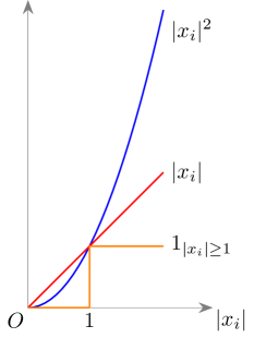
Figure 1: Comparison of different running-costs.

In this example, we aim at using Algorithms 1 and 2 to estimate the discounted value functions with respect to three types of running-costs. First, a quadratic function $r(x)=10\sum_{i=1}^{2}|x_{i}|^{2}$ is used, under which (9) reduces to a Lyapunov equation. Then, we select the $L^{1}$ vector norm $r(x)=10\sum_{i=1}^{2}|x_{i}|$. Finally, we choose $r(x)=10\sum_{i=1}^{2}1_{|x_{i}|\geq 1}$, which is essentially the 0-1 loss. See Figure 1 for an illustration of different choices of $r$. In all three cases, the discounting factor is fixed at $\gamma=1$, and the step size $\alpha_{t}$ in Algorithm 2 is chosen as $\alpha_{t}=0.7/(1+t)$. Model parameters of the OU process are chosen as $\theta_{1}=\theta_{2}=\sigma_{1}=\sigma_{2}=\sigma_{3}=1$, and the initial state is chosen as $x_{0}=(1,0)$. Six basis functions are selected: $\phi(x)=[1\ x_{1}\ x_{2}\ x_{1}^{2}\ x_{1}x_{2}\ x_{2}^{2}]$, where $x=(x_{1},x_{2})$.

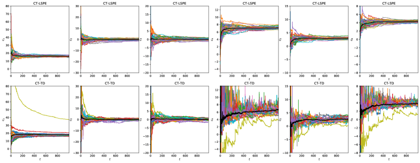
(a) $r(x)=10\sum_{i=1}^{2}|x_{i}|^{2}$.

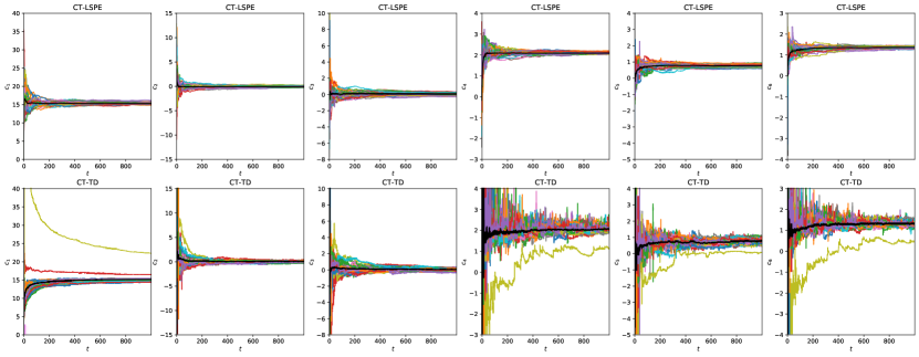
(b) $r(x)=10\sum_{i=1}^{2}|x_{i}|$.

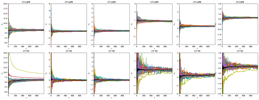
(c) $r(x)=10\sum_{i=1}^{2}1_{|x_{i}|\geq 1}$.

Figure 2: Value estimation for a continuous-time ARMA(2,1) process. The weights of basis functions ($\{c_{i,t}\}_{t\geq 0}$ for $i=1,2,\cdots,6$) along the 35 sample paths are plotted for the three choices of $r$. Each color, except black, is corresponding to one sample path. The solid black lines represent the point estimations of $c_{i,t}$.

Figures 2 and 3 show the experimental results of our algorithms. To evaluate the performance of the algorithms, we conduct learning processes over $35$ sample paths. Figure 2 illustrates the $35$ paths of the weights $\{c_{i}\}_{i=1}^{6}$ corresponding to the six basis functions. Figures 3(a), 3(b), and 3(c) show the box plots of these weights at $t=1000$. Overall, the weights obtained from both the CT-LSPE algorithm (Algorithm 1) and the CT-TD learning algorithm (Algorithm 2) converge to same values in all three cases. However, compared with the CT-LSPE, the CT-TD learning generates more dispersed samples, and the outliers are scattered further from the center of the clusters of samples. This is not surprising, as the time integration in the CT-LSPE tends to smooth out the noise in the learning process, especially at the beginning of the learning phase. Indeed, we can see from Figure 2 that CT-TD learning generates noisier paths of basis-function weights. To further illustrate the effectiveness of the proposed algorithms, we compare the value functions obtained from the two learning algorithms with that from Monte-Carlo (MC) simulations in Figures 3(d), 3(e), and 3(f). The point estimations of value functions at $t=1000$ with $95\%$ confidence intervals are given in Figures 3(g), 3(h), and 3(i). Note that in all three cases, these point estimations are approximately at the same level. In addition, compared with the CT-TD learning, the CT-LSPE produces a smaller standard error. This result is also consistent with the observations in Figures 3(a), 3(b), and 3(c). Finally, the MC simulation produces the largest standard error.

$r(x)=10\sum_{i=1}^{2}|x_{i}|^{2}$

$r(x)=10\sum_{i=1}^{2}|x_{i}|$

$r(x)=10\sum_{i=1}^{2}1_{|x_{i}|\geq 1}$

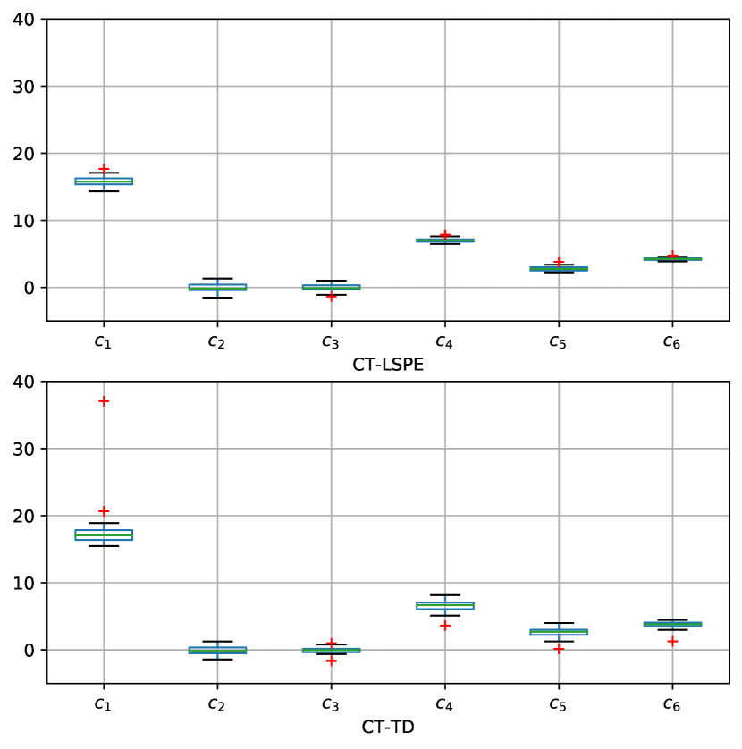
(a)

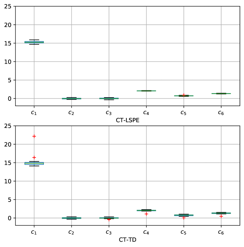
(b)

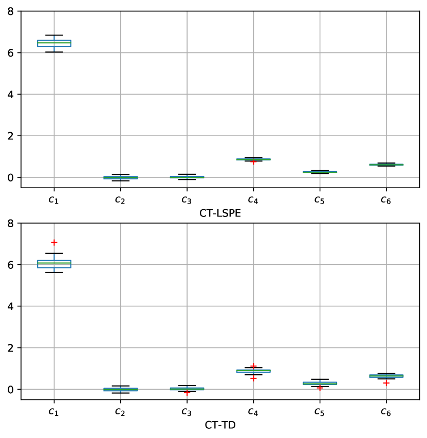
(c)

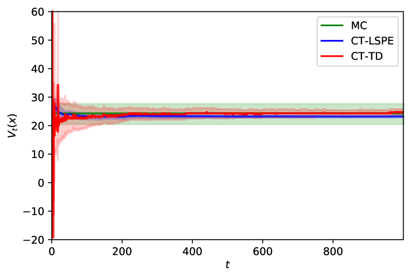
(d)

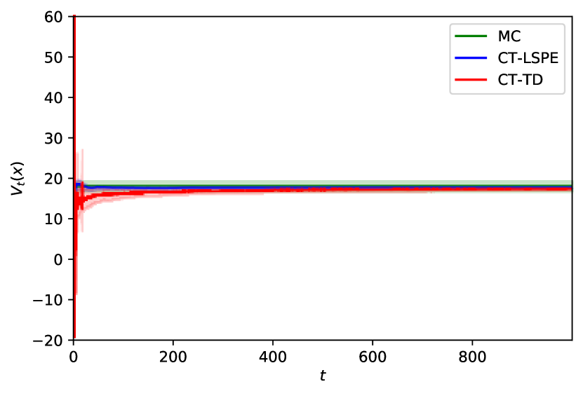
(e)

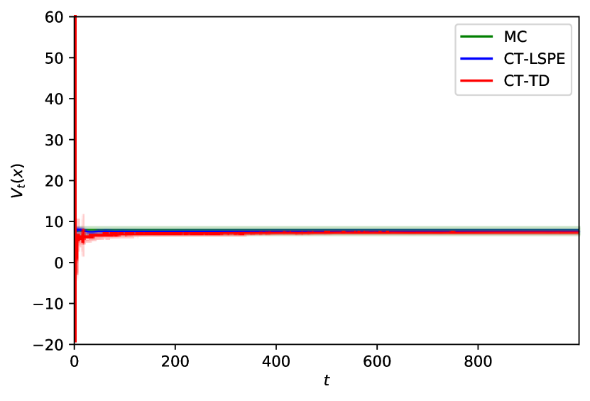
(f)

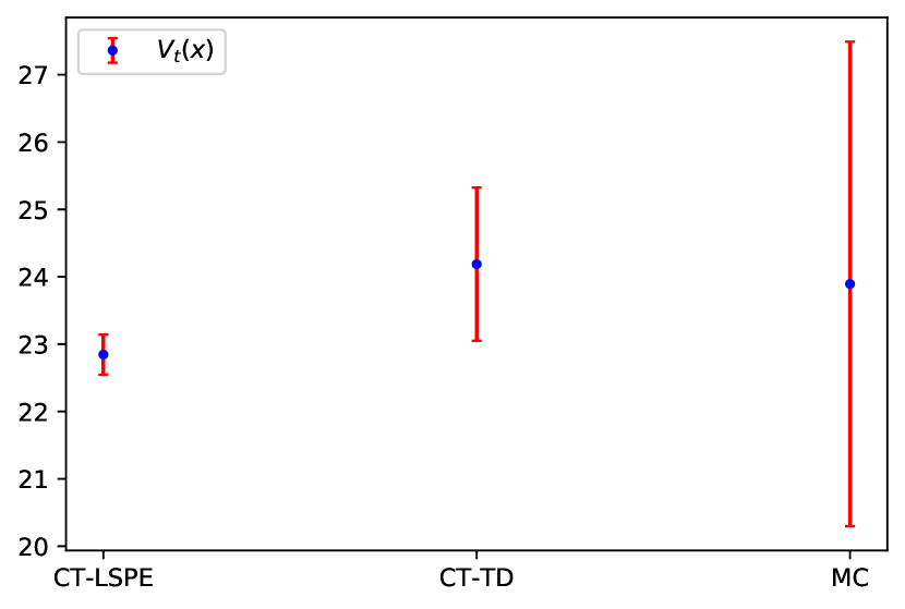
(g)

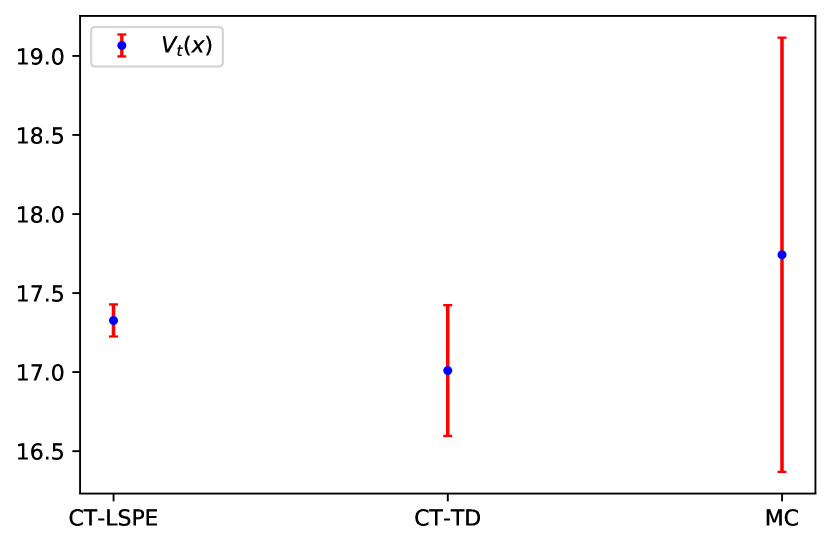
(h)

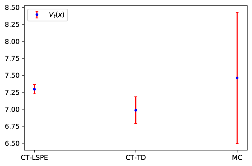
(i)

Figure 3: Value estimation for a continuous-time ARMA(2,1) process. Each one of the three columns in the figure is corresponding to one choice of $r$. Figures (a), (b), and (c) show the box plots of the basis-function weights ($\{c_{i,t}\}_{t\geq 0}$ for $i=1,2,\cdots,6$) at $t=1000$ along the $35$ sample paths. Figures (d), (e), and (f) show the estimations of the value functions ($V_{t}(x)$) at $x=(1,0)$. The solid lines represent point estimations of the true values using different algorithms. The shaded areas represent $95\%$ confidence intervals. Figures (g), (h), and (i) show the point estimations (blue dots) of $V_{1000}(x)$ at $x=(1,0)$ with $95\%$ confidence intervals (red bars) under different algorithms.

6.2 Control of the benchmark double inverted pendulum on a cart

In this example, we apply the CT-LSPE together with the actor-critic algorithm (Konda and Tsitsiklis, 2000) to improve the control performance of a double inverted pendulum on a cart (DIPC) (Figure 4). It is well-known that the DIPC is a nonlinear under-actuated plant, and designing a controller for DIPC is a challenging task in the field of nonlinear control (Khalil, 2015).

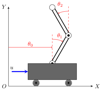
Figure 4: Double inverted-pendulum on a cart.

The mathematical model of the DIPC is given below (Moysis, 2016), which is derived from the Lagrange equations of the DIPC:

$$D(\theta)\ddot{\theta}+{C}(\theta,\dot{\theta})\dot{\theta}+{G}(\theta)=Hu,$$

where $\theta=[\theta_{0}\ \theta_{1}\ \theta_{2}]^{T}$, $\theta_{0}$ denotes the horizontal displacement of the cart, $\theta_{1}$ and $\theta_{2}$ denote the angles of lower and upper pendulum links with respect to the vertical position, respectively, $u$ is an input force applied to the cart, and

$$D(\theta) =\begin{bmatrix}C_{1}&C_{2}\cos\theta_{1}&{C_{3}\cos\theta_{2}}\\ {C_{2}\cos\theta_{1}}&{C_{4}}&{C_{5}\cos\left(\theta_{1}-\theta_{2}\right)}\\ C_{3}\cos\theta_{2}&C_{5}\cos\left(\theta_{1}-\theta_{2}\right)&{C_{6}}\end{bmatrix},\quad{G}(\theta)=\begin{bmatrix}{0}\\ {-C_{7}\sin\theta_{1}}\\ {-C_{8}\sin\theta_{2}}\end{bmatrix},$$

$${C}(\theta,\dot{\theta}) =\begin{bmatrix}{0}&{-C_{2}\sin\left(\theta_{1}\right)\dot{\theta}_{1}}&{-C_{3}\sin\left(\theta_{2}\right)\dot{\theta}_{2}}\\ {0}&{0}&{C_{5}\sin\left(\theta_{1}-\theta_{2}\right)\dot{\theta}_{2}}\\ 0&-C_{5}\sin\left(\theta_{1}-\theta_{2}\right)\dot{\theta}_{1}&{0}\end{bmatrix},\quad H=\begin{bmatrix}1\\ 0\\ 0\end{bmatrix},$$

$$C_{1} =m_{0}+m_{1}+m_{2},\quad C_{2}=\left(\frac{1}{2}m_{1}+m_{2}\right)l_{1},\quad C_{3}=\frac{1}{2}m_{2}l_{2},\quad C_{4}=\left(\frac{1}{3}m_{1}+m_{2}\right)l_{1}^{2},$$

$$C_{5} =\frac{1}{2}m_{2}l_{1}l_{2},\quad C_{6}=\frac{1}{3}m_{2}l_{2}^{2},\quad C_{7}=\left(\frac{1}{2}m_{1}+m_{2}\right)l_{1}g,\quad C_{8}=\frac{1}{2}m_{2}l_{2}g,$$

The model parameters are listed in Table 1.

Table 1: Parameters of the DIPC.

Parameters	Value	Definitions
$m_{0}$	1.5kg	Weight of the cart
$m_{1}$	0.5kg	Weight of the lower pendulum link
$m_{2}$	0.75kg	Weight of the upper pendulum link
$l_{1}$	0.5kg	Length of the lower pendulum link
$l_{2}$	0.75kg	Length of the upper pendulum link
$g$	9.81m/s2	Gravity constant

Denote the state of the DIPC as $x=[\theta_{0}\ \theta_{1}\ \theta_{2}\ \dot{\theta}_{0}\ \dot{\theta}_{1}\ \dot{\theta}_{2}]$. Now, we can rewrite the above model in the standard state-space form:

$$\dot{x}=\begin{bmatrix}0&I\\ 0&-D^{-1}C\end{bmatrix}x+\begin{bmatrix}0\\ -D^{-1}G\end{bmatrix}+\begin{bmatrix}0\\ -D^{-1}H\end{bmatrix}u.$$

Note that $D$, $C$, and $G$ are also nonlinear functions of $x$. Hence, the above system is an affine nonlinear system. In the learning task, at each state-action pair $(x,u)$, the following quadratic running cost is used

$$r(x,u)=x^{T}Qx+u^{2},\quad Q={\rm diag}\{100,\ 1000,\ 1000,\ 50,\ 10,\ 10\}.$$

We select basis functions as the 2nd order polynomials of $\theta_{0}$, $\theta_{1}$ and $\theta_{2}$ together with the constant function. Hence, there are totally $10$ bases in our learning algorithm. The initial state of the DIPC is at $(\theta_{0},\theta_{1},\theta_{2})=(0,10^{\circ},-10^{\circ})$. Here, we only consider linear controllers. In another word, we can always write $u_{t}=Kx_{t}$ for some real control gain matrix $K$.

The entire learning process is composed with $50$ learning trials, indexed by $k=1,2,\cdots,50$. Each learning trial is performed over a fixed time interval $[0,t_{f}]$. The initial controller parameter $K_{1}$ is adopted from Moysis (2016):

$$K_{1}=[-2.2361\ 499.6181\ -578.2160\ -8.2155\ 19.1832\ -88.4892].$$

The CT-LSPE algorithm is employed in each learning trial to estimate the value function. To facilitate the learning process, we add exploration noises in the system input in each learning trial. As a result, the control action applied to the DIPC in the $k$-th learning trial is $u_{t}=K_{k}x_{t}+{\rm noise}_{t}$, where $\text{noise}_{t}$ is a stationary Gaussian process with fixed distribution $\mathcal{N}(0,\sigma)$ for all $t\in[0,t_{f}]$. Then, $u_{t}$ has a distribution $\mathcal{N}(K_{k}x_{t},\sigma)\triangleq\pi_{k}(a_{t})$ in the $k$-th trial. Extending the actor-critic algorithm with eligibility trace in Konda (2002) to the continuous-time setting, we update the control gain matrix after finishing the $k$-th learning trial via

$$K_{k+1}=K_{k}-hz_{t_{f}}V_{t_{f}}(x_{0}),$$

where $h>0$ is the step size, $V_{t_{f}}$ is the value function learned in the $k$-th trial, and

$$z_{t}=\int_{0}^{t}\partial_{K_{k}}\left(\log\left(\pi_{k}(a_{s})\right)\right)ds\propto\int_{0}^{t}x_{s}^{T}\left(a_{s}-K_{k}x_{s}\right)ds$$

is the eligibility trace. Note that we only update the control gain matrix $K_{k}$ at the end of each learning trial in order to increase computational efficiency.

The experimental results are given in Figures 5 and 6. We fix $h=0.0005$ and ${t_{f}}=800$ during the learning process. After $50$ learning trials, the control gain matrix becomes

$$K_{50}=[-2.0547\ 498.9838\ -578.0119\ -16.9386\ 38.3267\ -90.5340].$$

The cost values $V_{t_{f}}(x_{0})$ estimated in each learning trial are plotted in Figure 5(a). Clearly the cost values show a decreasing trend as the trial number increases. We also plot the system trajectories under controllers $u_{1}=K_{1}x_{t}$ and $u_{50}=K_{50}x_{t}$ in Figure 5(b), respectively. Obviously, $u_{50}$ leads to a much better transient performance, in the sense that the DIPC shows less oscillations. Finally, the weights of basis functions ($\{c_{i,t}\}_{t\geq 0}$ for $i=1,2,\cdots,10$) before and after conducting the learning process are plotted in Figure 6.

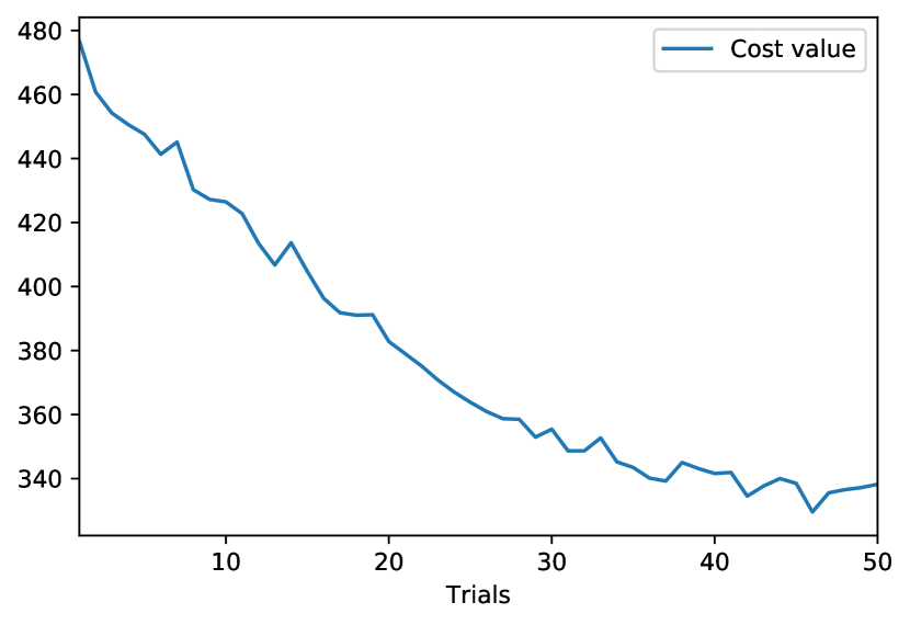
(a) Costs at different learning trials.

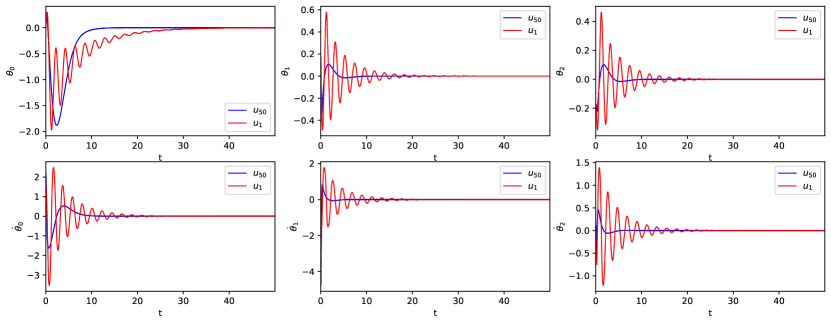
(b) Comparison between different controllers.

Figure 5: The value functions and system trajectories of DIPC, before and after conducting the learning process.

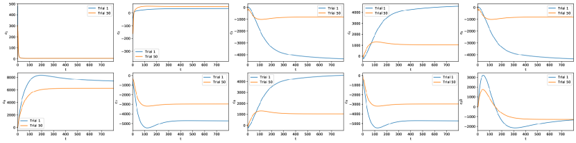
Figure 6: The weights of basis functions ($\{c_{i,t}\}_{t\geq 0}$ for $i=1,2,\cdots,10$) for the DIPC, in the first and the $50$-th learning trials.

7 Conclusions

This paper is motivated to provide a new RL framework for learning problems in continuous environments. A novel concept, known as the temporal-differential error, and a new class of temporal-differential learning methods, are proposed. In particular, two RL algorithms with detailed convergence analysis are designed for RL in continuous environments. Next, we point out several future research directions that deserve further investigations. First, the proposed algorithms are purely based on the temporal-differential error. It is interesting to see how to incorporate eligibility traces in RL algorithms driven by the temporal-differential error. Second, it is worth checking how to extend other existing discrete-time TD-learning-based RL algorithms to the continuous setting, by means of the techniques developed in this paper. Finally, besides the prediction problem which is the main focus of this paper, it is also important to investigate the off-policy learning problem in continuous environments.

Acknowledgments

The work of Z. P. Jiang has been supported partially by the National Science Foundation under Grants ECCS-1501044 and EPCN-1903781. The opinions expressed in this paper are those of the authors and do not necessarily reflect the views and policies of Bank of America.

A Review of Continuous-time Markov Processes

Let $(\Omega,\mathcal{F},\mathbb{P})$ be a probability space. Consider $\{x_{t}\}_{t\geq 0}$ as a homogeneous càdlàg (right continuous with left limits) strong Markov process on state space $X$, which is a locally compact Hausdorff space with a countable base and is equipped with the Borel $\sigma$-algebra $\mathcal{B}$. The definition of $X$ covers most spaces that will be encountered in RL tasks, including Euclidean spaces, countable discrete spaces, and topological manifolds. Starting with $x_{0}=x$, $x_{t}$ admits a stationary probability measure $\mu$ on $\mathcal{B}$. Denote by $\mathbb{E}_{x}$ the expectation conditionally on the initial state $x$ and by $\mathbb{E}_{\mu}$ the expectation with respect to $\mu$. $[M]_{t}$ denotes the quadratic variation of a real-valued stochastic process $M_{t}$ defined on $(\Omega,\mathcal{F},\mathbb{P})$.

Given the stationary distribution $\mu$, we can define a Hilbert space $L^{2}_{\mu}$ equipped with the inner product $\langle\cdot,\cdot\rangle_{\mu}$ and the norm $\|\cdot\|_{\mu}$:

$$\langle f,g\rangle_{\mu}=\int_{X}fg\ d\mu=\mathbb{E}_{\mu}\left[fg\right],\quad\|f\|_{\mu}=\sqrt{\langle f,f\rangle_{\mu}},\quad\forall f,\ g\in L^{2}_{\mu}.$$

In addition, we can define an operator $P_{t}:L^{2}_{\mu}\rightarrow L^{2}_{\mu}$ as

$$P_{t}f(x)=\mathbb{E}_{x}[f(x_{t})],\quad\forall x\in X.$$

One can easily check that $P_{t}$ is a contraction semigroup on $L^{2}_{\mu}$ (see Lemma 4 in Section C). In addition, the infinitesimal generator $\mathcal{A}$ associated with $P_{t}$ is defined as

$$\mathcal{A}f=\lim_{t\rightarrow 0}\frac{P_{t}f-f}{t},$$

provided that the above limit exists. Denote the domain and the range of $\mathcal{A}$ as $\mathcal{D}(\mathcal{A})\subseteq L^{2}_{\mu}$ and $\mathcal{R}(\mathcal{A})\subseteq L^{2}_{\mu}$, respectively. By Hille–Yosida theorem (Pazy, 1983), we know $\mathcal{A}$ is closed, and $\mathcal{D}(\mathcal{A})$ is a dense subset of $L^{2}_{\mu}$. Since $x_{t}$ is right continuous, its transition probability is stochastically continuous, and is uniquely determined by its infinitesimal generator. For additional properties on $P_{t}$ and $\mathcal{A}$, see Nelson (1958); Pazy (1983); Hansen and Scheinkman (1995).

B Proofs of Theorems

In this section, we present proofs of our three main theorems.

B.1 Proof of Theorem 1

We first show that $V_{t}$ exists on $\mathcal{H}$. For any $V\in\mathcal{H}$, we have from the definition of $K$ that

$$\langle V,\Pi\mathcal{A}V\rangle_{\mu} =\int_{X}V(x)\int_{X}(\mathcal{A}V)(z)K(z,x)d\mu(z)d\mu(x)$$

$$=\int_{X}(\mathcal{A}V)(z)\int_{X}V(x)K(x,z)d\mu(x)d\mu(z)$$

$$=\langle V,\mathcal{A}V\rangle_{\mu}.$$

Since $\mathcal{A}$ generates a contraction semigroup $P_{t}$ in $L^{2}_{\mu}$ (Lemma 4), we know by Lumer–Phillips theorem (Lumer and Phillips, 1961) that $\mathcal{A}$ is closed and dissipative. Hence, $\langle V,\mathcal{A}V\rangle_{\mu}\leq 0$. Thus, $\Pi\mathcal{A}$ is dissipative on $\mathcal{H}$, and $-\Pi\mathcal{A}$ is maximal monotone (Borwein, 2010, Proposition 1). Then, we have by Minty surjectivity theorem (Minty, 1962) that $\Pi\mathcal{A}-{\rm id}$ is surjective. In addition, since $\mathcal{A}$ is closed, we know by the definition of $\Pi$ and the dominated convergence theorem that $\Pi\mathcal{A}$ is closed on $\mathcal{H}$. Hence, again by Lumer–Phillips theorem, $\Pi\mathcal{A}$ generates a contraction semigroup on $\mathcal{H}$. Then we have from Phillips (1954) that the abstract Cauchy problem (3) admits a unique solution $V_{t}$. In addition, by Hille-Yosida theorem, $(\Pi\mathcal{A}-\gamma)^{-1}$ is bounded, and hence

$$0=\Pi(\mathcal{T}\hat{V}^{*}+r)=(\Pi\mathcal{A}-\gamma)\hat{V}^{*}+\Pi r$$

admits a unique solution $\hat{V}^{*}$ on $\mathcal{H}$.

Denote $\tilde{V}_{t}=V_{t}-\hat{V}^{*}$. We next show that $V_{t}$ converges to $\hat{V}^{*}$ exponentially. Note from (3) and the above analysis that

$$\frac{d}{dt}\left\|\tilde{V}_{t}(x)\right\|_{\mu}^{2}=2\int_{X}\tilde{V}_{t}(x)\int_{X}\left(\mathcal{A}\tilde{V}_{t}-\gamma\tilde{V}_{t}\right)(z)K(z,x)d\mu(z)d\mu(x)\leq-2\gamma\left\|\tilde{V}_{t}\right\|_{\mu}^{2}.$$

This implies that $V_{t}$ is globally exponentially stable at $\hat{V}^{*}$.

Now, to derive the first finite-time error bound, we have

$$\left\|V_{t}-V^{*}\right\|_{\mu}\leq\left\|V_{t}-\hat{V}^{*}\right\|_{\mu}+\left\|\hat{V}^{*}-V^{*}\right\|_{\mu}\leq e^{-\gamma t}\left\|V_{0}-\hat{V}^{*}\right\|_{\mu}+\left\|\hat{V}^{*}-V^{*}\right\|_{\mu}.$$

Denote $0=\mathcal{T}(\hat{V}^{*})+r+\varepsilon$, where $\varepsilon$ is the approximation error due to $\Pi$. Using Dynkin’s formula and the tower property, we have

$$\hat{V}^{*}(x) =\mathbb{E}_{x}\left[e^{-\gamma t}\hat{V}^{*}(x_{t})+\int_{0}^{t}e^{-\gamma s}(r(x_{s})+\varepsilon(x_{s}))ds\right],$$

$$V^{*}(x) =\mathbb{E}_{x}\left[e^{-\gamma t}V^{*}(x_{t})+\int_{0}^{t}e^{-\gamma s}r(x_{s})ds\right].$$

Since $\mu$ is the stationary distribution, we have by Jenson’s inequality and Fubini’s theorem that

$$\gamma^{2}\left\|\hat{V}^{*}-V^{*}\right\|_{\mu}^{2}=\mathbb{E}_{\mu}\left[\left|\mathbb{E}_{x}\left[\int_{0}^{\infty}\gamma e^{-\gamma s}\varepsilon(x_{s})ds\right]\right|^{2}\right] \leq\mathbb{E}_{\mu}\left[\int_{0}^{\infty}\gamma e^{-\gamma s}\varepsilon^{2}(x_{s})ds\right]$$

$$=\left\|\mathcal{T}(\hat{V}^{*})+r\right\|_{\mu}^{2}.$$

To derive the second finite-time error bound, we rewrite (3) as

$$\partial_{t}V_{t}(x)=\mathcal{T}V_{t}(x)+r(x)+\varepsilon_{t}(x),$$

where $\varepsilon_{t}$ is the approximation error at time $t$. Using Dynkin’s formula, we have

$$V_{t}(x) =\mathbb{E}_{x}\left[e^{-\gamma t}V_{0}(x_{t})+\int_{0}^{t}e^{-\gamma s}(r(x_{s})+\varepsilon_{t-s}(x_{s}))ds\right],$$

and hence

$$V_{t}(x)-V^{*}(x) =\mathbb{E}_{x}\left[e^{-\gamma t}(V_{0}-V^{*})(x_{t})+\int_{0}^{t}e^{-\gamma s}\varepsilon_{t-s}(x_{s})ds\right].$$

Then,

$$\quad\frac{\gamma}{1-e^{-\gamma t}}\left\|V_{t}-V^{*}\right\|_{\mu}$$

$$\leq\frac{\gamma e^{-\gamma t}}{1-e^{-\gamma t}}\left\|\mathbb{E}_{x}\left[(V_{0}-V^{*})(x_{t})\right]\right\|_{\mu}+\left\|\mathbb{E}_{x}\left[\int_{0}^{t}\frac{\gamma e^{-\gamma s}}{1-e^{-\gamma t}}\varepsilon_{t-s}(x_{s})ds\right]\right\|_{\mu}$$

$$=\frac{\gamma e^{-\gamma t}}{1-e^{-\gamma t}}\sqrt{\mathbb{E}_{\mu}\left[\left|\mathbb{E}_{x}\left[(V_{0}-V^{*})(x_{t})\right]\right|^{2}\right]}+\sqrt{\mathbb{E}_{\mu}\left[\left|\mathbb{E}_{x}\left[\int_{0}^{t}\frac{\gamma e^{-\gamma s}}{1-e^{-\gamma t}}\varepsilon_{t-s}(x_{s})ds\right]\right|^{2}\right]}$$

$$\leq\frac{\gamma e^{-\gamma t}}{1-e^{-\gamma t}}\sqrt{\mathbb{E}_{\mu}\left[\left|(V_{0}-V^{*})(x_{t})\right|^{2}\right]}+\sqrt{\mathbb{E}_{\mu}\left[\left|\int_{0}^{t}\frac{\gamma e^{-\gamma s}}{1-e^{-\gamma t}}\varepsilon_{t-s}(x_{s})ds\right|^{2}\right]}$$ (10)

$$\leq\frac{\gamma e^{-\gamma t}}{1-e^{-\gamma t}}\left\|V_{0}-V^{*}\right\|_{\mu}+\sqrt{\int_{0}^{t}\frac{\gamma e^{-\gamma s}}{1-e^{-\gamma t}}\|\varepsilon_{t-s}\|_{\mu}^{2}ds}$$ (11)

$$=\frac{\gamma e^{-\gamma t}}{1-e^{-\gamma t}}\left\|V_{0}-V^{*}\right\|_{\mu}+\sqrt{\int_{0}^{t}\frac{\gamma e^{-\gamma(t-s)}}{1-e^{-\gamma t}}\left\|(\Pi-{\rm id})(\mathcal{T}V_{s}+r)\right\|_{\mu}^{2}ds}$$

$$\leq\frac{\gamma e^{-\gamma t}}{1-e^{-\gamma t}}\left\|V_{0}-V^{*}\right\|_{\mu}+\sup_{s\in[0,t]}\left\|(\Pi-{\rm id})(\mathcal{T}V_{s}+r)\right\|_{\mu},$$

where (10) and (11) above are due to Jenson’s inequality. This completes the proof.

B.2 Proof of Theorem 2

We first show $R_{t}=\left(\int_{0}^{t}\phi_{s}\phi^{T}_{s}ds+\rho I\right)^{-1}$. Since

$$\frac{d}{dt}\left(R_{t}\left(\int_{0}^{t}\phi_{s}\phi^{T}_{s}ds+\rho I\right)\right)=\dot{R}_{t}\left(\int_{0}^{t}\phi_{s}\phi^{T}_{s}ds+\rho I\right)+R_{t}\phi_{t}\phi^{T}_{t},$$

$R_{t}=\left(\int_{0}^{t}\phi_{s}\phi^{T}_{s}ds+\rho I\right)^{-1}$ solves the ODE of $R_{t}$ in Algorithm 1. Since the right-hand-side of the ODE of $R_{t}$ is locally Lipschitz, and $\left(\int_{0}^{t}\phi_{s}\phi^{T}_{s}ds+\rho I\right)^{-1}$ is bounded, we can select a sufficiently large subset $S$ of the space of all symmetric positive definite matrices, such that $R_{t}=\left(\int_{0}^{t}\phi_{s}\phi^{T}_{s}ds+\rho I\right)^{-1}$ is a unique solution of the ODE of $R_{t}$ on $S$, and it also remains in $S$.

We next denote

$$A_{t} \triangleq\frac{1}{t+1}\int_{0}^{t}\phi_{s}(\mathcal{A}\phi_{s}-\gamma\phi_{s})^{T}ds,\quad b_{t}\triangleq\frac{1}{t+1}\int_{0}^{t}\phi_{s}r_{s}ds,$$

$$\Sigma_{t} \triangleq\frac{1}{t+1}\left(\int_{0}^{t}\phi_{s}\phi^{T}_{s}ds+\rho I\right),\quad\eta_{t}\triangleq\frac{1}{t+1}\int_{0}^{t}\phi_{s}dM_{s}^{T}.$$

Then, we can rewrite the updating equation of $c_{t}$ in Algorithm 1 as

$$\dot{c}_{t}=\Sigma^{-1}Ac_{t}+\Sigma^{-1}b+(\Sigma_{t}^{-1}A_{t}-\Sigma^{-1}A)c_{t}+\Sigma_{t}^{-1}b_{t}-\Sigma^{-1}b+\Sigma_{t}^{-1}\eta_{t}c_{t},$$ (12)

where

$$A \triangleq\int_{X}\phi(\mathcal{A}\phi-\gamma\phi)^{T}d\mu,\quad b\triangleq\int_{X}\phi rd\mu,\quad\Sigma\triangleq\int_{X}\phi\phi^{T}d\mu.$$

Let $\tilde{c}_{t}=c_{t}-c^{*}$. Then,

$$\dot{\tilde{c}}_{t}=\Sigma^{-1}A\tilde{c}_{t} +\left(\Sigma_{t}^{-1}A_{t}-\Sigma^{-1}A+\Sigma_{t}^{-1}\eta_{t}\right)\tilde{c}_{t}+\Sigma_{t}^{-1}b_{t}-\Sigma^{-1}b+\left(\Sigma_{t}^{-1}A_{t}-\Sigma^{-1}A+\Sigma_{t}^{-1}\eta_{t}\right)c^{*}.$$

By Assumptions 2, we have

$$\mathcal{A}\psi_{i}(x_{s})=\Delta_{i,s},$$

where $i=2,3,4$, $\psi_{4}=\psi_{1}-\gamma\psi_{3}$, and

$$\Delta_{2,s}=\phi(x_{s})\phi^{T}(x_{s})-\Sigma,\quad\Delta_{3,s}=\phi(x_{s})r(x_{s})-b,\quad\Delta_{4,s} =\phi(x_{s})(\mathcal{A}\phi^{T}(x_{s})-\gamma\phi^{T}(x_{s}))-A.$$

Then, we have by Lemma 6 (element-wise) that

$$\lim_{t\rightarrow\infty}\mathbb{E}_{x}\left[\psi_{i}(x_{t})\right]=0,\quad\sup_{t\geq 0}\frac{1}{t+1}\mathbb{E}_{x}\left[\left|\int_{0}^{t}\Delta_{i,s}ds\right|^{2}\right]<\infty,\quad i=2,3,4.$$

Now consider the boundedness of $\eta_{t}$. The quadratic variation of the $j$-th element in $M_{t}$ is given below:

$$d[M_{j}]_{t} =(dM_{j,t})^{2}=(d\phi_{j}(x_{t}))^{2}+O(dt^{2}).$$

By Assumption 3 and Ito’s isometry, we have

$$\sup_{t\geq 0}(t+1)\mathbb{E}_{x}\left[\left|\eta_{t}\right|^{2}\right]<\infty.$$

Applying Lemma 5 with $\alpha_{t}=1/\sqrt{t+1}$, we know with probability one that $A_{t}$, $b_{t}$, and $\Sigma_{t}$ converge to $A$, $b$, and $\Sigma$, respectively. In addition, we know with a probability at least of $1-C_{0}/\epsilon^{2}$ that

$$|A_{t}-A|\leq\frac{\epsilon}{\sqrt{t+1}},\quad|b_{t}-b|\leq\frac{\epsilon}{\sqrt{t+1}},\quad|\Sigma_{t}-\Sigma|\leq\frac{\epsilon}{\sqrt{t+1}},\quad\text{and}\quad|\eta_{t}|\leq\frac{\epsilon}{\sqrt{t+1}},$$

for all $t\geq 0$, where

$$C_{0}=\sup_{t\geq 0}\max\left\{(t+1)\mathbb{E}_{x}\left[\left|\eta_{t}\right|^{2}\right],\ \frac{1}{t+1}\mathbb{E}_{x}\left[\left|\int_{0}^{t}\Delta_{i,s}ds\right|^{2}\right],\ i=2,3,4\right\}.$$

As a result, by the boundedness of $A_{t}$, $b_{t}$, $\Sigma_{t}$, and $\eta_{t}$, we have with a probability at least $1-C_{0}/\epsilon^{2}$ that

$$\left|\Sigma_{t}^{-1}\right| \leq{\rho_{0}},\quad\left|I-\Sigma\Sigma_{t}^{-1}\right|\leq\left|\Sigma_{t}-\Sigma\right|\left|\Sigma_{t}^{-1}\right|\leq\frac{\epsilon\rho_{0}}{t+1},$$

$$\left|\Sigma\Sigma_{t}^{-1}\right| \leq 1+\frac{\epsilon\rho_{0}}{t+1},\quad\left|\Sigma\Sigma_{t}^{-1}\eta_{t}\right|\leq\frac{\epsilon\left(1+\epsilon\rho_{0}\right)}{\sqrt{t+1}},$$

$$\left|\Sigma\Sigma_{t}^{-1}A_{t}-A\right| \leq\left|\Sigma\Sigma_{t}^{-1}\right|\left|A_{t}-A\right|+\left|\Sigma\Sigma_{t}^{-1}-I\right|\left|A\right|\leq\frac{\epsilon}{\sqrt{t+1}}\left(\epsilon\rho_{0}+\rho_{0}|A|+1\right),$$

$$\left|\Sigma\Sigma_{t}^{-1}b_{t}-b\right| \leq\frac{\epsilon}{\sqrt{t+1}}\left(\epsilon\rho_{0}+\rho_{0}\left|b\right|+1\right),$$

where

$$\rho_{0}=\frac{\epsilon+|\Sigma|}{|\Sigma|^{2}}+\frac{\left(\epsilon+|\Sigma|\right)^{2}}{\rho|\Sigma|^{2}}.$$

Applying Lemma 7, we know $c_{t}$ converges to $c^{*}$ with probability one. In addition,

$$\left|c_{t}-c^{*}\right|^{2}\leq\frac{\lambda_{M}}{\lambda_{m}}e^{\zeta(t,0)}\left|c_{0}-c^{*}\right|^{2}+\frac{\lambda_{M}}{\varepsilon\lambda_{m}}\int_{0}^{t}\xi(s)e^{\zeta(t,s)}ds$$

with a probability at least $1-C_{0}/\epsilon^{2}$, where $\lambda_{M}$ and $\lambda_{m}$ represent the largest and the smallest eigenvalues of $\Sigma$, respectively, $\varepsilon<2\gamma/\lambda_{M}$ is an arbitrary positive constant, and by Lemma 9,

$$\zeta(t,s) =-\left(\frac{2\gamma}{\lambda_{M}}-\varepsilon\right)(t-s)+4\epsilon\left(2+2\epsilon\rho_{0}+\rho_{0}\left|A\right|\right)\left(\sqrt{t+1}-\sqrt{s+1}\right)$$

$$\leq-2\left(\frac{\gamma}{\lambda_{M}}-\varepsilon\right)(t-s)+C_{1},$$

$$\xi(s) =\frac{C_{2}}{s+1},$$

where

$$C_{1}=\varepsilon+\frac{4\epsilon^{2}\left(2+2\epsilon\rho_{0}+\rho_{0}\left|A\right|\right)^{2}}{\varepsilon},\quad C_{2}=\epsilon^{2}\left(\rho_{0}\left(\left|b\right|+\left|A\right||c^{*}|\right)+(1+\epsilon\rho_{0})(1+2|c^{*}|)\right)^{2}.$$

In particular, we know by Lemma 10 that $\left|c_{t}-c^{*}\right|^{2}=O\left(t^{-1}\right)$. This completes the proof.

B.3 Proof of Theorem 3

First, we introduce the following auxillary system:

$$\dot{\hat{c}}_{t}=\alpha_{t}(A\hat{c}_{t}+b),\quad\hat{c}_{0}=c_{0},$$

where $A$ and $b$ follow the definitions in Appendix B.2.

We first show that $\hat{c}_{t}$ converges to $c^{*}$. Indeed, a direct calculation shows that

$$\frac{d}{dt}\left|\hat{c}_{t}-c^{*}\right|^{2}=2\alpha_{t}(\hat{c}_{t}-c^{*})^{T}A(\hat{c}_{t}-c^{*})\leq-2\gamma\alpha_{t}|\hat{c}_{t}-c^{*}|^{2}.$$

By the comparison lemma (Sontag, 1998, Lemma C.3.1), we have

$$|\hat{c}_{t}-c^{*}|^{2}\leq e^{-2\gamma\int_{0}^{t}\alpha_{s}ds}|\hat{c}_{0}-c^{*}|^{2}.$$

Since $\int_{0}^{\infty}\alpha_{t}dt=\infty$, $\hat{c}_{t}$ converges to $c^{*}$ as $t$ goes to the infinity.

Denote $\tilde{c}=c-\hat{c}$. We can rewrite the updating equation in Algorithm 2 as

$$d\tilde{c}_{t}=\alpha_{t}(A\tilde{c}_{t}+\Delta_{4,t}\tilde{c}_{t}+\Delta_{4,t}\hat{c}_{t}+\Delta_{3,t})dt+\alpha_{t}\phi(x_{t})(\tilde{c}_{t}+\hat{c}_{t})^{T}dM_{t},\quad\tilde{c}_{0}=0,$$

where $\Delta_{3,t}$ and $\Delta_{4,t}$ follow the definitions in Appendix B.2.

Note that $c^{T}dM=\sum_{j}c_{j}dM_{j}$, where $dM_{j}$ denotes the $j$-th element in $dM$. Now the proof is completed by applying Lemma 8.

C Technical Lemmas

In this section, we present several supporting lemmas that have been used in the proofs of our main results.

Lemma 4

$P_{t}$ is a contraction semigroup in $L^{2}_{\mu}$.

Proof  We have by Jenson’s inequality that

$$\|P_{t}f\|_{\mu}^{2}=\int_{X}|P_{t}f(x)|^{2}d\mu(x)\leq\int_{X}P_{t}(f^{2})(x)d\mu(x)=\int_{X}f^{2}(x)d\mu(x)=\|f\|_{\mu}^{2},\quad\forall f\in L^{2}_{\mu}.$$

This completes the proof.  

Lemma 5

Suppose $S_{t}$ is a time series satisfying

$$\alpha_{t}^{2}\mathbb{E}\left[S_{t}^{2}\right]\leq C,\quad\forall t\geq 0,$$

for some $C<\infty$, where $\alpha_{t}>0$ is deterministic and decreases monotonically to $0$. Then, for any $\epsilon>\sqrt{C}$,

$$\mathbb{P}\left(\sup_{t\geq 0}\left|\alpha_{t}S_{t}\right|<\epsilon\right)>1-\frac{1}{\epsilon^{2}}C.$$

In particular, $\alpha_{t}^{2}S_{t}=O({\alpha_{t}})$ with probability one.

Proof  Denote events

$$E_{T}=\left\{\max_{0\leq t\leq T}\left|{\alpha_{t}}S_{t}\right|>\epsilon\right\},\quad\forall T\geq 0.$$

By Markov’s inequality, $\mathbb{P}\left(E_{T}\right)\leq{C}/{\epsilon^{2}}$. Since $E_{T}$ is increasing, by monotone convergence theorem,

$$\lim_{T\rightarrow\infty}\mathbb{P}\left(E_{T}\right)=\mathbb{P}\left(\lim_{T\rightarrow\infty}E_{T}\right)=\mathbb{P}\left(\sup_{t\geq 0}\left|{\alpha_{t}}S_{t}\right|>\epsilon\right)\leq\frac{1}{\epsilon^{2}}C.$$

Letting $\epsilon$ go to the infinity, we have

$$\mathbb{P}\left(\sup_{t\geq 0}\left|{\alpha_{t}}S_{t}\right|<\infty\right)=1.$$

This completes the proof.  

Lemma 6

Suppose Assumption 1 holds. Denote by $\psi$ the solution to the following Poisson equation:

$$\mathcal{A}\psi(x_{t})=f(x_{t})-\mathbb{E}_{\mu}[f].$$

Then,

$$\lim_{t\rightarrow\infty}\mathbb{E}_{x}\left[\psi(x_{t})\right]=0,\quad\limsup_{t\rightarrow\infty}\frac{1}{t}\mathbb{E}_{x}\left[\left|\int_{0}^{t}\mathcal{A}\psi(x_{t})dt\right|^{2}\right]<\infty.$$

Proof  Since $\psi\in\mathcal{D}(\mathcal{A})$, $\mathbb{E}_{\mu}\left[\psi^{2}\right]<\infty$ and $\mathbb{E}_{\mu}\left[f^{2}\right]<\infty$. By Assumption 1 and the ergodic theorems (Kontoyiannis and Meyn, 2003, Theorem 2.2 and Corollary 2.3),

$$\lim_{t\rightarrow\infty}\mathbb{E}_{x}\left[\psi(x_{t})\right]=\mathbb{E}_{\mu}[\psi]=0,\quad\lim_{t\rightarrow\infty}\mathbb{E}_{x}\left[f^{2}(x_{t})\right]=\mathbb{E}_{\mu}\left[f^{2}\right].$$

Denote

$$m_{t}=\psi(x_{t})-\psi(x)+\int_{0}^{t}\mathcal{A}\psi(x_{s})ds.$$

Then $m$ is a martingale, and we have by the martingale property that

$$\mathbb{E}_{x}[m_{t}^{2}]=\mathbb{E}_{x}\left[\left(\sum_{i}\Delta m_{i,t}\right)^{2}\right]=\sum_{i}\mathbb{E}_{x}[(\Delta m_{i,t})^{2}]=\sum_{i}\mathbb{E}_{x}\left[\left(\frac{\Delta m_{i,t}}{\sqrt{\Delta t_{i}}}\right)^{2}\Delta t_{i}\right],$$

where $0=t_{1}<t_{2}<\cdots=t$ is a set of partition points on the interval $[0,t]$, $\Delta t_{i}=t_{i+1}-t_{i}$, and

$$\Delta m_{i,t}=\psi(x_{t_{i+1}})-\psi(x_{t_{i}})+\int_{t_{i}}^{t_{i+1}}\mathcal{A}\psi(x_{s})ds.$$

We next quantify $\mathbb{E}_{x}[m_{t}^{2}]$ by inspecting $\mathbb{E}_{x}[\Delta m_{i,t}^{2}]$. By Hölder’s inequality,

$$\mathbb{E}_{x}\left[\left(\frac{1}{\sqrt{\Delta t_{i}}}\int_{t_{i}}^{t_{i+1}}\mathcal{A}\psi(x_{s})ds\right)^{2}\right]\leq\int_{t_{i}}^{t_{i+1}}\mathbb{E}_{x}\left[\left(\mathcal{A}\psi(x_{s})\right)^{2}\right]ds=O(\Delta t_{i}),$$

where the last equality holds since the integrand is bounded. In addition,

$$\quad\mathbb{E}_{x}\left[\left(\psi(x_{t_{i+1}})-\psi(x_{t_{i}})\right)^{2}\right]$$

$$=\mathbb{E}_{x}\left[\psi^{2}(x_{t_{i+1}})-2\psi(x_{t_{i+1}})\psi(x_{t_{i}})+\psi^{2}(x_{t_{i}})\right]$$

$$=\mathbb{E}_{x}\left[\psi^{2}(x_{t_{i+1}})\right]+\mathbb{E}_{x}\left[\psi^{2}(x_{t_{i}})\right]-2\mathbb{E}_{x}\left[P_{\Delta t_{i}}\psi(x_{t_{i}})\psi(x_{t_{i}})\right]$$

$$=\mathbb{E}_{x}\left[\psi^{2}(x_{t_{i+1}})\right]-\mathbb{E}_{x}\left[\psi^{2}(x_{t_{i}})\right]-2\mathbb{E}_{x}\left[(P_{\Delta t_{i}}-{\rm id})\psi(x_{t_{i}})\psi(x_{t_{i}})\right]$$

$$=\mathbb{E}_{x}\left[\psi^{2}(x_{t_{i+1}})\right]-\mathbb{E}_{x}\left[\psi^{2}(x_{t_{i}})\right]-2\Delta t_{i}\mathbb{E}_{x}\left[\frac{(P_{\Delta t_{i}}-{\rm id})\psi(x_{t_{i}})}{\Delta t_{i}}\psi(x_{t_{i}})\right].$$

Putting the above items back into the summation in $\mathbb{E}_{x}[m_{t}^{2}]$ and letting $\Delta t_{i}$ go to $0$, we have

$$\mathbb{E}_{x}[m_{t}^{2}]=\mathbb{E}_{x}\left[\psi^{2}(x_{t})\right]-\psi^{2}(x)-2\int_{0}^{t}\mathbb{E}_{x}\left[\mathcal{A}\psi(x_{s})\psi(x_{s})\right]ds.$$

Since both $\psi$ and $f$ are square integrable, $\limsup_{t\rightarrow\infty}t^{-1}\mathbb{E}_{x}[m_{t}^{2}]<\infty$. This completes the proof.  

Lemma 7

Consider the following system:

$$\dot{c}_{t}=(\Sigma^{-1}A+\Delta A_{t})c_{t}+\Delta_{t},$$

where $\Sigma$ is a symmetric positive definite matrix, $A$ is a negative definite real matrix, and $\Delta A_{t}$ and $\Delta_{t}$ are random variables bounded with probability one. Assume

$$\lim_{t\rightarrow\infty}\frac{1}{t}\int_{0}^{t}\left|\Delta A_{s}\right|ds=0$$

for all $\omega\in E\in\mathcal{F}$. Then $c$ is input-to-state stable (ISS) (Sontag, 2008) over $E$, from $\Delta_{t}$ to $c_{t}$.

Proof  Consider the Lyapunov function $V(c)=c^{T}\Sigma c$. Given $\omega\in E$,

$$\dot{V}(c_{t}) =-c_{t}^{T}(A+A^{T})c_{t}+2c_{t}^{T}\Sigma\Delta A_{t}c_{t}+2c_{t}^{T}\Sigma\Delta_{t}$$

$$\leq-(\gamma-\varepsilon|\Sigma|-2|\Sigma||\Delta A_{t}|)|c_{t}|^{2}+\frac{1}{\varepsilon}\Delta_{t}^{T}\Sigma\Delta_{t}$$

$$\leq-(\gamma|\Sigma|^{-1}-\varepsilon-2|\Delta A_{t}|)V(c_{t})+\frac{1}{\varepsilon}\Delta_{t}^{T}\Sigma\Delta_{t},$$

where $\gamma>0$ satisfies $A^{T}+A\leq-\gamma I$, and $\varepsilon<\gamma|\Sigma|^{-1}$ is a positive constant. Reformulating the above inequality, we have

$$\frac{d}{dt}\left(V(c_{t})e^{(\gamma|\Sigma|^{-1}-\varepsilon)t-2\int_{0}^{t}|\Delta A_{s}|ds}\right)\leq\frac{|\Sigma|}{\varepsilon}|\Delta_{t}|^{2}e^{(\gamma|\Sigma|^{-1}-\varepsilon)t-2\int_{0}^{t}|\Delta A_{s}|ds}.$$

Hence,

$$\left|c_{t}\right|^{2}\leq\frac{\lambda_{M}}{\lambda_{m}}e^{-(|\gamma/\lambda_{M}-\varepsilon)t+2\int_{0}^{t}|\Delta A_{s}|ds}\left|c_{0}\right|^{2}+\frac{\lambda_{M}}{\varepsilon\lambda_{m}}\int_{0}^{t}e^{-(\gamma/\lambda_{M}-\varepsilon)(t-s)+2\int_{s}^{t}|\Delta A_{\tau}|d\tau}\left|\Delta_{s}\right|^{2}ds.$$

where $\lambda_{M}$ and $\lambda_{m}$ represent the largest and the smallest eigenvalues of $\Sigma$, respectively. One can see from the above inequality and our assumption on $\Delta A$ that $c_{t}$ is ISS, from $\Delta_{t}$ to $c_{t}$. This completes the proof.  

Lemma 8

Consider the following system:

$$dc_{t}=\alpha_{t}(Ac_{t}+\Delta_{1,t}c_{t}+\Delta_{2,t})dt+\alpha_{t}\sum_{j=1}^{N}g_{j,t}(c_{t})dM_{j,t},$$ (13)

where $A$ is a real matrix satisfying $A+A^{T}<-2\gamma I$ for some $\gamma>0$, $\alpha_{t}>0$ is continuously differentiable with $\dot{\alpha}_{t}\leq 0$, $\lim_{t\rightarrow\infty}\alpha_{t}=0$ and $\int_{0}^{\infty}\alpha_{t}=\infty$, $g_{j}$ is a vector-valued function, $M_{j}$ is a real-valued martingale, and $\Delta_{1,t}$ and $\Delta_{2,t}$ are random variables that are bounded with probability one and satisfy

$$d\psi_{i,t}=\Delta_{i,t}dt+dm_{i,t},\quad\mathbb{E}_{\mu}\left[\Delta_{i,t}\right]=0,$$

for some martingales $m_{i}$, $i=1,2$. In addition, $M_{j}$ and $m_{i}$ are adapted to a filtration $\{\mathcal{F}_{t}\}_{t\geq 0}$, and there exist a function $\varphi$ and a constant $C>0$, such that $d[M_{j}]_{t}\leq\varphi_{t}dt$ and $d[m_{i,k}]_{t}\leq\varphi_{t}dt$ for the $k$-th elements in $m_{i}$, and

$$\mathbb{E}_{0}\left[|\Delta_{i,t}|^{4}\right]\leq C,\quad\mathbb{E}_{0}\left[|\psi_{i,t}|^{4}\right]\leq C,\quad\mathbb{E}_{0}\left[\varphi_{t}^{4}\right]\leq C,\quad\mathbb{E}_{0}\left[\left|\frac{g_{j,t}(c)}{1+|c|}\right|^{8}\right]\leq C,$$

for all $c$, where $\mathbb{E}_{0}$ denotes the expectation conditional on $\mathcal{F}_{0}$.

Given the above conditions, we have

$$\mathbb{P}\left(\left|c_{t}\right|^{2}<\epsilon\left(\left|c_{0}\right|^{2}+\sqrt{A_{n}C_{0}}b^{2}e^{2\lambda(n+1)}\right)e^{-2\gamma\int_{0}^{t}\alpha_{s}ds}\right)>1-A_{n}C_{0}-\frac{2}{\epsilon},$$

where $b=\max\left\{1,|c_{0}|\right\}$,

$$A_{n} =\alpha_{n}^{2}+\left(\int_{n}^{\infty}\alpha_{t}^{2}dt\right)^{2}+\int_{n}^{\infty}\alpha_{t}^{2}dt,$$

$$\lambda =\frac{\alpha_{0}\left(b^{2}+1\right)^{1/\epsilon}}{2\left(b^{2}+1\right)^{1/\epsilon}-2}\left(2\sqrt[4]{C}+(2\alpha_{0}N^{2}+1)\sqrt{C}+1\right)+\frac{\log 2}{2},$$

$C_{0}$ is a positive constant, and $n$ and $\epsilon$ are sufficiently large integers and reals, respectively.

Proof  The proof contains three parts. First, we show $|c_{t}|$ cannot grow faster than the exponential rate. Second, we show $|c_{t}|$ is bounded. Finally, we show $|c_{t}|$ is asymptotically stable at the origin.

First, given $\lambda>0$ and $b=\max\{1,|c_{0}|\}$, we define $B_{b}=\left\{\omega\in\Omega:|c_{t}(\omega)|<be^{\lambda t}\ \text{for all $t$}\right\}$ and

$$\sigma_{n}(\omega)=\inf\left\{t:\left|c_{t}(\omega)\right|=be^{\lambda n}\right\},\quad\tau_{n}(\omega)=\sup\left\{t<\sigma_{n+1}(\omega):\left|c_{t}(\omega)\right|=be^{\lambda n}\right\},\quad n\geq 1.$$

Then, $\sigma_{n}\leq\tau_{n}<\sigma_{n+1}$. Obviously, for any $\omega\in B_{b}$, we have $\sigma_{n}(\omega)\geq n$ for all $n$. Denote $E_{n}=\{\omega\in\Omega:\sigma_{n}(\omega)<\infty\}$, $E_{n,b}=\{\omega\in B_{b}:\sigma_{n}(\omega)<\infty\}$, and $\mathbb{E}_{0}^{E}[Y]=\mathbb{E}_{0}\left[Y\cdot 1_{\omega\in E}\right]$ for any $E\in\mathcal{F}$ and randome variable $Y$. Note that for any measurable function $f\geq 0$, $\mathbb{E}_{0}^{E}[f]=\mathbb{E}_{0}\left[f\cdot 1_{\omega\in E}\right]\leq\mathbb{E}_{0}\left[f\right]$.

Denote $z_{t}=e^{-\lambda t}c_{t}$. Then,

$$dz_{t}=-\lambda z_{t}+\alpha_{t}(Az_{t}+\Delta_{1,t}z_{t}+e^{-\lambda t}\Delta_{2,t})dt+\alpha_{t}e^{-\lambda t}\sum_{j=1}^{N}g_{j,t}(c_{t})dM_{j,t},$$

Define $V(z)=\log\left(|z|^{2}+1\right)$. Then the Hessian of $V$ is

$$\frac{2(|z|^{2}+1)I-4zz^{T}}{(|z|^{2}+1)^{2}}\leq\frac{2}{|z|^{2}+1}I\leq\frac{4}{(|z|+1)^{2}}I,$$

and we have for any $|z_{t}|\geq\delta$, where $0<\delta\leq b$, that

$$\mathcal{A}V(z_{t}) \leq-\frac{2\lambda\delta^{2}}{1+\delta^{2}}+\bar{\Delta}_{t}.$$

where

$$\bar{\Delta}_{t} =\alpha_{t}\left(2|\Delta_{1,t}|+1+|\Delta_{2,t}|^{2}\right)+2\alpha_{t}^{2}N\sum_{j=1}^{N}\frac{|g_{j,t}(c_{t})|^{2}\varphi_{t}}{(|c_{t}|+1)^{2}}.$$

By Dynkin’s formula, whenever $|z_{\sigma}|\geq\delta$ for some $\sigma\geq 0$, one has

$$\mathbb{E}_{\sigma}[V(z_{\min(t,\tau_{\sigma})})]\leq V(z_{\sigma})+\mathbb{E}_{\sigma}\int_{\sigma}^{\min(t,\tau_{\sigma})}\left(-\frac{2\lambda\delta^{2}}{1+\delta^{2}}+\bar{\Delta}_{s}\right)ds,$$

where $\tau_{\sigma}$ is the first time after $\sigma$ at which $z_{\tau_{\sigma}}$ exists $\{z:|z|\geq\delta\}$. By the definition of $\lambda$, $\sup_{t}\mathbb{E}_{0}[\bar{\Delta}_{t}]<{2\lambda\delta^{2}}(1+\delta^{2})^{-1}$. Now, we have from the tower property that $\sup_{t}\mathbb{E}_{0}\left[V(z_{t})\right]\leq V(z_{0})$. Thus, by Markov’s inequality, one has

$$\mathbb{P}\left(B_{b}\right)=\mathbb{P}\left(V(z_{t})<\log(b^{2}+1)\right)>1-\frac{\log\left(\delta^{2}+1\right)}{\log(b^{2}+1)},\quad\forall t\geq 0.$$

Hence, $z_{t}$ is bounded with probability one.

Now, we show $|c_{t}|$ is bounded. On one hand, we have on $E_{n+1}$ that

$$\left|c_{\sigma_{n+1}}\right|^{2}-\left|c_{\tau_{n}}\right|^{2}=b^{2}e^{2\lambda(n+1)}-b^{2}e^{2\lambda n}\geq b^{2}e^{2\lambda n}>0.$$ (14)

On the other hand, we can derive that

$$\quad d\left(\frac{1}{2}|c_{t}|^{2}-\alpha_{t}c_{t}^{T}(\psi_{1,t}c_{t}+\psi_{2,t})\right)$$

$$=c_{t}^{T}dc_{t}+\frac{1}{2}dc_{t}^{T}dc_{t}-d\alpha_{t}c_{t}^{T}(\psi_{1,t}c_{t}+\psi_{2,t})-\alpha_{t}dc_{t}^{T}(\psi_{1,t}c_{t}+\psi_{2,t})$$

$$\quad-\alpha_{t}c_{t}^{T}(\psi_{1,t}dc_{t}+d\psi_{1,t}c_{t}+d\psi_{2,t})-\alpha_{t}dc_{t}^{T}(\psi_{1,t}dc_{t}+d\psi_{1,t}c_{t}+d\psi_{2,t})-\alpha_{t}c_{t}^{T}d\psi_{1,t}dc_{t}$$

$$\leq\alpha_{t}c_{t}^{T}(Ac_{t}+\Delta_{1,t}c_{t}+\Delta_{2,t})dt+\alpha_{t}c_{t}^{T}\sum_{j=1}^{N}g_{j,t}(c_{t})dM_{j,t}+\alpha_{t}^{2}\frac{N}{2}\sum_{j=1}^{N}|g_{j,t}(c_{t})|^{2}\varphi_{t}dt$$

$$\quad-\dot{\alpha}_{t}c_{t}^{T}(\psi_{1,t}c_{t}+\psi_{2,t})dt-\alpha_{t}c_{t}^{T}(d\psi_{1,t}c_{t}+d\psi_{2,t})$$

$$\quad-\alpha_{t}(2(\psi_{1,t}+d\psi_{1,t})c_{t}+(\psi_{2,t}+d\psi_{2,t}))^{T}dc_{t}-\alpha_{t}dc_{t}^{T}\psi_{1,t}dc_{t}$$

$$\leq-\alpha_{t}c_{t}^{T}(dm_{1,t}c_{t}+dm_{2,t})+\alpha_{t}c_{t}^{T}\sum_{j=1}^{N}g_{j,t}(c_{t})dM_{j,t}+\alpha_{t}^{2}\frac{N}{2}\sum_{j=1}^{N}|g_{j,t}(c_{t})|^{2}\varphi_{t}dt$$

$$\quad-\dot{\alpha}_{t}c_{t}^{T}(\psi_{1,t}c_{t}+\psi_{2,t})dt-\alpha_{t}^{2}(2\psi_{1,t}c_{t}+\psi_{2,t})^{T}(Ac_{t}+\Delta_{1,t}c_{t}+\Delta_{2,t})dt$$

$$\quad-\alpha_{t}^{2}(2\psi_{1,t}c_{t}+\psi_{2,t})^{T}\sum_{j=1}^{N}g_{j,t}(c_{t})dM_{j,t}+\alpha_{t}^{3}N|\psi_{1,t}|\sum_{j=1}^{N}|g_{j,t}(c_{t})|^{2}\varphi_{t}dt$$

$$\quad+\alpha_{t}^{2}|c_{t}|^{2}\sum_{k=1}^{N^{2}}\left(dm_{1,k,t}\right)^{2}+\alpha_{t}^{2}\frac{3N}{2}\sum_{j=1}^{N}|g_{j,t}(c_{t})|^{2}\varphi_{t}dt+\frac{1}{2}\alpha_{t}^{2}|d\psi_{2,t}|^{2},$$

where $m_{1,k}$ is the $k$-th element in $m_{1}$. Taking integration on both sides of the above inequality, we have for any $\omega\in E_{n+1}$ that

$$0 <\frac{1}{2}\left(|c_{\sigma_{n+1}}|^{2}-|c_{\tau_{n}}|^{2}\right)$$

$$\leq\alpha_{\sigma_{n+1}}c_{\sigma_{n+1}}^{T}(\psi_{1,{\sigma_{n+1}}}c_{\sigma_{n+1}}+\psi_{2,{\sigma_{n+1}}})-\alpha_{\tau_{n}}c_{\tau_{n}}^{T}(\psi_{1,{\tau_{n}}}c_{\tau_{n}}+\psi_{2,{\tau_{n}}})-\int_{\tau_{n}}^{\sigma_{n+1}}\alpha_{t}c_{t}^{T}dm_{1,t}c_{t}$$

$$\quad-\int_{\tau_{n}}^{\sigma_{n+1}}\alpha_{t}c_{t}^{T}dm_{2,t}+N\sum_{j=1}^{N}\int_{\tau_{n}}^{\sigma_{n+1}}\alpha_{t}^{2}\left(2+\alpha_{t}|\psi_{1,t}|\right)|g_{j,t}(c_{t})|^{2}\varphi_{t}dt$$

$$\quad-\int_{\tau_{n}}^{\sigma_{n+1}}\dot{\alpha}_{t}c_{t}^{T}(\psi_{2,t}+\psi_{1,t}c_{t})dt-2\int_{\tau_{n}}^{\sigma_{n+1}}\alpha_{t}^{2}c_{t}^{T}\psi_{1,t}^{T}(A+\Delta_{1,t})c_{t}dt$$

$$\quad-\int_{\tau_{n}}^{\sigma_{n+1}}\alpha_{t}^{2}c_{t}^{T}(2\psi_{1,t}^{T}\Delta_{2,t}+(A+\Delta_{1,t})^{T}\psi_{2,t})dt-\int_{\tau_{n}}^{\sigma_{n+1}}\alpha_{t}^{2}\psi_{2,t}^{T}\Delta_{2,t}dt$$

$$\quad+\sum_{j=1}^{N}\int_{\tau_{n}}^{\sigma_{n+1}}\alpha_{t}c_{t}^{T}(1-2\alpha_{t}\psi_{1,t}^{T})g_{j,t}(c_{t})dM_{j,t}-\sum_{j=1}^{N}\int_{\tau_{n}}^{\sigma_{n+1}}\alpha_{t}^{2}\psi_{2,t}^{T}g_{j,t}(c_{t})dM_{j,t}$$

$$\quad+\sum_{k=1}^{N^{2}}\int_{\tau_{n}}^{\sigma_{n+1}}\alpha_{t}^{2}|c_{t}|^{2}\left(dm_{1,k,t}\right)^{2}+\frac{1}{2}\sum_{k=1}^{N}\int_{\tau_{n}}^{\sigma_{n+1}}\alpha_{t}^{2}\left(dm_{2,k,t}\right)^{2}.$$

Note that for all $\omega\in E_{n+1,b}$, $n\leq\tau_{n}<\sigma_{n+1}<\infty$ and $|c_{t}|<be^{\lambda(n+1)}$ for $\tau_{n}\leq t<\sigma_{n+1}$. Then, we have by Young’s inequality, Hölder’s inequality, and the definitions of $\alpha$, $\sigma_{n}$, and $\tau_{n}$ that

$$\quad\frac{1}{56}\left||c_{\sigma_{n+1}}|^{2}-|c_{\tau_{n}}|^{2}\right|^{2}$$

$$\leq\alpha_{\sigma_{n+1}}^{2}\left|c_{\sigma_{n+1}}^{T}(\psi_{1,{\sigma_{n+1}}}c_{\sigma_{n+1}}+\psi_{2,{\sigma_{n+1}}})\right|^{2}+\alpha_{\tau_{n}}^{2}\left|c_{\tau_{n}}^{T}(\psi_{1,{\tau_{n}}}c_{\tau_{n}}+\psi_{2,{\tau_{n}}})\right|^{2}$$

$$\quad+\left|\int_{\tau_{n}}^{\sigma_{n+1}}\alpha_{t}c_{t}^{T}dm_{1,t}c_{t}\right|^{2}+\left|\int_{\tau_{n}}^{\sigma_{n+1}}\alpha_{t}c_{t}^{T}dm_{2,t}\right|^{2}$$

$$\quad+N^{3}\sum_{j=1}^{N}\left|\int_{\tau_{n}}^{\sigma_{n+1}}\alpha_{t}^{2}\left(2+\alpha_{t}|\psi_{1,t}|\right)|g_{j,t}(c_{t})|^{2}\varphi_{t}dt\right|^{2}+\left|\int_{\tau_{n}}^{\sigma_{n+1}}\dot{\alpha}_{t}c_{t}^{T}\psi_{2,t}dt\right|^{2}$$

$$\quad+\left|\int_{\tau_{n}}^{\sigma_{n+1}}\dot{\alpha}_{t}c_{t}^{T}\psi_{1,t}c_{t}dt\right|^{2}+4\left|\int_{\tau_{n}}^{\sigma_{n+1}}\alpha_{t}^{2}c_{t}^{T}\psi_{1,t}^{T}(A+\Delta_{1,t})c_{t}dt\right|^{2}$$

$$\quad+\left|\int_{\tau_{n}}^{\sigma_{n+1}}\alpha_{t}^{2}c_{t}^{T}\left(2\psi_{1,t}^{T}\Delta_{2,t}+(A+\Delta_{1,t})^{T}\psi_{2,t}\right)dt\right|^{2}+\left|\int_{\tau_{n}}^{\sigma_{n+1}}\alpha_{t}^{2}\psi_{2,t}^{T}\Delta_{2,t}dt\right|^{2}$$

$$\quad+N\sum_{j=1}^{N}\left|\int_{\tau_{n}}^{\sigma_{n+1}}\alpha_{t}c_{t}^{T}\left(1-2\alpha_{t}\psi_{1,t}^{T}\right)g_{j,t}(c_{t})dM_{j,t}\right|^{2}+N\sum_{j=1}^{N}\left|\int_{\tau_{n}}^{\sigma_{n+1}}\alpha_{t}^{2}\psi_{2,t}^{T}g_{j,t}(c_{t})dM_{j,t}\right|^{2}$$

$$\quad+N^{2}\sum_{k=1}^{N^{2}}\left|\int_{\tau_{n}}^{\sigma_{n+1}}\alpha_{t}^{2}|c_{t}|^{2}\left(dm_{1,k,t}\right)^{2}\right|^{2}+\frac{N}{4}\sum_{k=1}^{N}\left|\int_{\tau_{n}}^{\sigma_{n+1}}\alpha_{t}^{2}\left(dm_{2,k,t}\right)^{2}\right|^{2}$$

$$\leq 2\alpha_{\sigma_{n+1}}^{2}\left(|\psi_{1,{\sigma_{n+1}}}|^{2}b^{4}e^{4\lambda(n+1)}+|\psi_{2,{\sigma_{n+1}}}|^{2}b^{2}e^{2\lambda(n+1)}\right)$$

$$\quad+2\alpha_{\tau_{n}}^{2}\left(|\psi_{1,{\tau_{n}}}|^{2}b^{4}e^{4\lambda(n+1)}+|\psi_{2,{\tau_{n}}}|^{2}b^{2}e^{2\lambda(n+1)}\right)+\left|\int_{\tau_{n}}^{\sigma_{n+1}}\alpha_{t}c_{t}^{T}dm_{1,t}c_{t}\right|^{2}$$

$$\quad+\left|\int_{\tau_{n}}^{\sigma_{n+1}}\alpha_{t}c_{t}^{T}dm_{2,t}\right|^{2}+2N^{3}\sum_{j=1}^{N}\int_{\tau_{n}}^{\sigma_{n+1}}\alpha_{t}^{2}dt\int_{\tau_{n}}^{\sigma_{n+1}}\alpha_{t}^{2}\left(4+\alpha_{t}^{2}|\psi_{1,t}|^{2}\right)|g_{j,t}(c_{t})|^{4}\varphi_{t}^{2}dt$$

$$\quad+\int_{\tau_{n}}^{\sigma_{n+1}}\dot{\alpha}_{t}dt\int_{\tau_{n}}^{\sigma_{n+1}}\dot{\alpha}_{t}|\psi_{2,t}|^{2}dtb^{2}e^{2\lambda(n+1)}+\int_{\tau_{n}}^{\sigma_{n+1}}\dot{\alpha}_{t}dt\int_{\tau_{n}}^{\sigma_{n+1}}\dot{\alpha}_{t}|\psi_{1,t}|^{2}dtb^{4}e^{4\lambda(n+1)}$$

$$\quad+4\int_{\tau_{n}}^{\sigma_{n+1}}\alpha_{t}^{2}dt\int_{\tau_{n}}^{\sigma_{n+1}}\alpha_{t}^{2}\left|\psi_{1,t}^{T}(A+\Delta_{1,t})\right|^{2}dtb^{4}e^{4\lambda(n+1)}$$

$$\quad+\int_{\tau_{n}}^{\sigma_{n+1}}\alpha_{t}^{2}dt\int_{\tau_{n}}^{\sigma_{n+1}}\alpha_{t}^{2}\left|2\psi_{1,t}^{T}\Delta_{2,t}+(A+\Delta_{1,t})^{T}\psi_{2,t}\right|^{2}dtb^{2}e^{2\lambda(n+1)}$$

$$\quad+\int_{\tau_{n}}^{\sigma_{n+1}}\alpha_{t}^{2}dt\int_{\tau_{n}}^{\sigma_{n+1}}\alpha_{t}^{2}\left|\psi_{2,t}^{T}\Delta_{2,t}\right|^{2}dt+N\sum_{j=1}^{N}\left|\int_{\tau_{n}}^{\sigma_{n+1}}\alpha_{t}c_{t}^{T}\left(1-2\alpha_{t}\psi_{1,t}^{T}\right)g_{j,t}(c_{t})dM_{j,t}\right|^{2}$$

$$\quad+N\sum_{j=1}^{N}\left|\int_{\tau_{n}}^{\sigma_{n+1}}\alpha_{t}^{2}\psi_{2,t}^{T}g_{j,t}(c_{t})dM_{j,t}\right|^{2}+N^{2}\sum_{k=1}^{N^{2}}\left|\int_{\tau_{n}}^{\sigma_{n+1}}\alpha_{t}^{2}\left(dm_{1,k,t}\right)^{2}\right|^{2}b^{4}e^{4\lambda(n+1)}$$

$$\quad+\frac{N}{4}\sum_{k=1}^{N}\left|\int_{\tau_{n}}^{\sigma_{n+1}}\alpha_{t}^{2}\left(dm_{2,k,t}\right)^{2}\right|^{2}.$$

Taking expectations on both sides of the above inequality, we have by Ito’s isometry and Fubini’s theorem that

$$\quad\frac{1}{56}\mathbb{E}_{0}^{E_{n+1,b}}\left[\left||c_{\sigma_{n+1}}|^{2}-|c_{\tau_{n}}|^{2}\right|^{2}\right]$$

$$\leq 2\alpha_{n}^{2}\sup_{t\geq 0}\mathbb{E}_{0}\left[|\psi_{1,t}|^{2}+|\psi_{2,t}|^{2}\right]b^{4}e^{4\lambda(n+1)}+2\alpha_{n}^{2}\sup_{t\geq 0}\mathbb{E}_{0}\left[|\psi_{1,t}|^{2}+|\psi_{2,t}|^{2}\right]b^{4}e^{4\lambda(n+1)}$$

$$\quad+N^{2}\int_{n}^{\infty}\alpha_{t}^{2}dt\mathbb{E}_{0}\left[\varphi_{t}^{2}\right]b^{4}e^{4\lambda(n+1)}+N\int_{n}^{\infty}\alpha_{t}^{2}dt\mathbb{E}_{0}\left[\varphi_{t}^{2}\right]b^{2}e^{2\lambda(n+1)}$$

$$\quad+2N^{4}\left(\int_{n}^{\infty}\alpha_{t}^{2}dt\right)^{2}\sup_{t\geq 0,j\geq 1}\mathbb{E}_{0}\left[\left(4+\alpha_{n}^{2}|\psi_{1,t}|^{2}\right)\frac{|g_{j,t}(c_{t})|^{4}}{(1+|c_{t}|)^{4}}\varphi_{t}^{2}\right]\left(1+be^{\lambda(n+1)}\right)^{4}$$

$$\quad+\alpha_{n}^{2}\sup_{t\geq 0}\mathbb{E}_{0}\left[|\psi_{2,t}|^{2}\right]b^{2}e^{2\lambda(n+1)}+\alpha_{n}^{2}\sup_{t\geq 0}\mathbb{E}_{0}\left[|\psi_{1,t}|^{2}\right]b^{4}e^{4\lambda(n+1)}$$

$$\quad+4\left(\int_{n}^{\infty}\alpha_{t}^{2}dt\right)^{2}\sup_{t\geq 0}\mathbb{E}_{0}\left[\left|\psi_{1,t}^{T}(A+\Delta_{1,t})\right|^{2}\right]b^{4}e^{4\lambda(n+1)}$$

$$\quad+\left(\int_{n}^{\infty}\alpha_{t}^{2}dt\right)^{2}\sup_{t\geq 0}\mathbb{E}_{0}\left[\left|2\psi_{1,t}^{T}\Delta_{2,t}+(A+\Delta_{1,t})^{T}\psi_{2,t}\right|^{2}\right]b^{2}e^{2\lambda(n+1)}$$

$$\quad+\left(\int_{n}^{\infty}\alpha_{t}^{2}dt\right)^{2}\sup_{t\geq 0}\mathbb{E}_{0}\left[\left|\psi_{2,t}^{T}\Delta_{2,t}\right|^{2}\right]$$

$$\quad+N^{2}\int_{n}^{\infty}\alpha_{t}^{2}dt\sup_{t\geq 0,j\geq 1}\mathbb{E}_{0}\left[(1-2\alpha_{t}\psi_{1,t}^{T})^{2}\frac{|g_{j,t}(c_{t})|^{2}}{(1+|c_{t}|)^{2}}\varphi_{t}\right]\left(1+be^{\lambda(n+1)}\right)^{2}b^{2}e^{2\lambda(n+1)}$$

$$\quad+N^{2}\int_{n}^{\infty}\alpha_{t}^{4}dt\sup_{t\geq 0,j\geq 1}\mathbb{E}_{0}\left[|\psi_{2,t}|^{2}\frac{|g_{j,t}(c_{t})|^{2}}{(1+|c_{t}|)^{2}}\varphi_{t}\right]\left(1+be^{\lambda(n+1)}\right)^{2}$$

$$\quad+N^{4}\left(\int_{n}^{\infty}\alpha_{t}^{2}dt\right)^{2}\mathbb{E}_{0}\left[\varphi_{t}^{2}\right]b^{4}e^{4\lambda(n+1)}+\frac{N^{2}}{4}\left(\int_{\tau_{n}}^{\sigma_{n+1}}\alpha_{t}^{2}dt\right)^{2}\mathbb{E}_{0}\left[\varphi_{t}^{2}\right].$$ (15)

Hence, we can deduce from (15) that there exists $C_{0}>0$, so that

$$\mathbb{E}_{0}^{E_{n+1,b}}\left[\left|\left|c_{\sigma_{n+1}}\right|^{2}-\left|c_{\tau_{n}}\right|^{2}\right|^{2}\right]\leq C_{0}A_{n}b^{4}e^{4\lambda(n+1)},$$ (16)

where

$$A_{n}=\alpha_{n}^{2}+\left(\int_{n}^{\infty}\alpha_{t}^{2}dt\right)^{2}+\int_{n}^{\infty}\alpha_{t}^{2}dt.$$

As a result, we have from (14) and (16) that

$$\mathbb{P}\left({E_{n+1,b}}\right)\leq C_{0}A_{n}e^{4\lambda},\quad n\geq 1.$$

Thus, we have

$$\mathbb{P}\left(\overline{E}_{n+1}\right)\geq\mathbb{P}(B_{b}\setminus E_{n+1,b})>1-\frac{\log\left(\delta^{2}+1\right)}{\log(b^{2}+1)}-C_{0}A_{n}e^{4\lambda}.$$

In particular, this implies that $\mathbb{P}\left(\sup_{t\geq 0}|c_{t}|<\infty\right)=1$.

Now we can write

$$\mathbb{E}_{0}^{\overline{E}_{n+1}}\left[\left|c_{t}\right|^{2}\right]\leq\left|c_{0}\right|^{2}-2\gamma\int_{0}^{t}\alpha_{s}\mathbb{E}_{0}^{\overline{E}_{n+1}}\left[\left|c_{s}\right|^{2}\right]ds+\sqrt{C_{0}A_{n}}b^{2}e^{2\lambda n}.$$

By the comparison lemma (Sontag, 1998, Lemma C.3.1), we have

$$\mathbb{E}_{0}^{\overline{E}_{n+1}}\left[\left|c_{t}\right|^{2}\right]\leq\left(\left|c_{0}\right|^{2}+\sqrt{C_{0}A_{n}}b^{2}e^{2\lambda n}\right)e^{-2\gamma\int_{0}^{t}\alpha_{s}ds}.$$

By Markov’s inequality, one has for all $\epsilon>1$ that

$$\mathbb{P}\left(\omega\in\overline{E}_{n+1}:\left|c_{t}(\omega)\right|^{2}\geq\epsilon\left(\left|c_{0}\right|^{2}+\sqrt{C_{0}A_{n}}b^{2}e^{2\lambda(n+1)}\right)e^{-2\gamma\int_{0}^{t}\alpha_{s}ds}\right)\leq\frac{1}{\epsilon}.$$

Hence,

$$\quad\mathbb{P}\left(\omega\in\Omega:\left|c_{t}(\omega)\right|^{2}<\epsilon\left(\left|c_{0}\right|^{2}+\sqrt{C_{0}A_{n}}b^{2}e^{2\lambda(n+1)}\right)e^{-2\gamma\int_{0}^{t}\alpha_{s}ds}\right)$$

$$>\mathbb{P}\left(\omega\in\overline{E}_{n+1}:\left|c_{t}(\omega)\right|^{2}<\epsilon\left(\left|c_{0}\right|^{2}+\sqrt{C_{0}A_{n}}b^{2}e^{2\lambda(n+1)}\right)e^{-2\gamma\int_{0}^{t}\alpha_{s}ds}\right)$$

$$>1-\frac{\log\left(\delta^{2}+1\right)}{\log(b^{2}+1)}-C_{0}A_{n}e^{4\lambda}-\frac{1}{\epsilon}.$$

Denote $\epsilon^{-1}=\frac{\log\left(\delta^{2}+1\right)}{\log(b^{2}+1)}$. Then,

$$\delta^{2}=e^{\log(\delta^{2}+1)}-1=e^{{\epsilon^{-1}\log\left(b^{2}+1\right)}}-1=\left(b^{2}+1\right)^{1/\epsilon}-1.$$

This completes the proof.  

Lemma 9

For any $0\leq s<t$, $a>0$ and $b>0$, we have

$$at-\sqrt{t+b} \geq as-\sqrt{s+b}-ab-\frac{1}{4a}.$$

Proof  Denote $y_{t}=at-\sqrt{t+b}$. Then

$$\dot{y}_{t}=a-\frac{1}{2\sqrt{t+b}}.$$

If $a>(2\sqrt{b})^{-1}$, then $\dot{y}_{t}>0$ for all $t$. As a result, $y_{t}>y_{s}$ for all $t>s$. If $a\leq(2\sqrt{b})^{-1}$, then $y_{t}-y_{s}\geq\min_{t}y_{t}-y_{0}$, where $\min_{t}y_{t}=-ab-(4a)^{-1}$. This completes the proof.  

Lemma 10

Suppose $a$ is a positive real. Then for any $t_{0}>0$,

$$\int_{t_{0}}^{t}\frac{1}{s}e^{as}ds\leq\frac{h}{t}e^{at}$$

for some $h>0$.

Proof  First, consider the following auxiliary dynamical system defined on $[t_{0},\infty)$:

$$\dot{x}_{t} =z_{t}\quad x_{t_{0}}=0,$$

$$\dot{z}_{t} =-\frac{1}{t}z_{t}+az_{t},\quad z_{t_{0}}=\frac{1}{t_{0}}e^{at_{0}}.$$

To complete the proof, we only need to show $x_{t}<hz_{t}$ for some $h>0$. Denote $e=x-hz$, where $h>0$ is a sufficiently large constant that will be determined later. Then $e_{t_{0}}<0$, and we have

$$\dot{e} =\dot{x}-h\dot{z}=z_{t}+\frac{h}{t}z_{t}-ahz_{t}=z_{t}\left(1+\frac{h}{t}-ah\right).$$

Now, if $a>t_{0}^{-1}$, we can choose $h>(a-t_{0}^{-1})^{-1}$, such that $1+ht^{-1}-ah<0$ for all $t\geq t_{0}$. Since $z_{t}>0$, we have $\dot{e}_{t}<0$, and as a result $x_{t}<hz_{t}$ for all $t\geq t_{0}$.

If $a\leq t_{0}^{-1}$, then $1+ht^{-1}-ah=0$ admits a solution $t=t^{\prime}\triangleq\frac{h}{ah-1}>t_{0}$ for all $h>a^{-1}$. Hence, $e_{t}$ reaches its maximum at $t=t^{\prime}$. As a result, we can choose

$$h\geq\frac{1}{ae}\int_{t_{0}}^{\frac{2}{a}}\frac{1}{s}e^{as}ds+\frac{2}{a},$$

which implies that

$$\int_{t_{0}}^{\frac{h}{ha-1}}\frac{1}{s}e^{as}ds\leq(ha-1)e^{\frac{1}{ha-1}+1},$$

and hence $e_{t_{0}}\leq 0$. This completes the proof.  

Lemma 11

Consider $\alpha_{t}>0$ with $\dot{\alpha}_{t}\leq 0$. If there exist $h>0$ and $t_{0}\geq 0$, such that $\alpha_{t}^{2}\geq-h\dot{\alpha}_{t}$ for all $t\geq t_{0}$, then

$$e^{-\int_{t_{0}}^{t}\alpha_{s}ds}\leq\left(\frac{\alpha_{t}}{\alpha_{t_{0}}}\right)^{h}.$$

Proof  By definition,

$$\alpha_{t}\geq-h\frac{\dot{\alpha}_{t}}{\alpha_{t}}\geq 0,\quad\forall t\geq t_{0}.$$

Taking integration from $t_{0}$ to $t$, we have

$$\int_{t_{0}}^{t}\alpha_{s}ds\geq h\log(\alpha_{t_{0}})-h\log(\alpha_{t}).$$

Hence,

$$e^{-\int_{t_{0}}^{t}\alpha_{s}ds}\leq\left(\frac{\alpha_{t}}{\alpha_{t_{0}}}\right)^{h}.$$

This completes the proof.

References

- Antos et al. (2008) A. Antos, C. Szepesvári, and R. Munos. Fitted Q-iteration in continuous action-space MDPs. In Advances in Neural Information Processing Systems 20, pages 9–16. Curran Associates, Inc., 2008.
- Arapostathis et al. (2012) A. Arapostathis, V. S. Borkar, and M. K. Ghosh. Ergodic Control of Diffusion Processes. Cambridge University Press, New York, NY, 2012.
- Arnold (1974) L. Arnold. Stochastic Differential Equations: Theory and Applications. John Wiley & Sons, Inc., New York, 1974.
- Aronszajn (1950) N. Aronszajn. Theory of reproducing kernels. Transactions of the American Mathematical Society, 68(3):337–404, 1950.
- Baird, III (1993) L. C. Baird, III. Advantage updating. Technical Report WL–TR-93-1146, Wright-Patterson Air Force Base Ohio: Wright Laboratory, Washington DC, 1993.
- Barto et al. (2017) A. G. Barto, P. S. Tomas, and R. S. Sutton. Some recent applications of reinforcement learning. In Proceedings of the Eighteenth Yale Workshop on Adaptive and Learning Systems, 2017.
- Benveniste et al. (1990) A. Benveniste, M. Métivier, and P. Priouret. Adaptive algorithms and stochastic approximations. Springer Berlin Heidelberg, 1990.
- Bhattacharya (1982) R. N. Bhattacharya. On the functional central limit theorem and the law of the iterated logarithm for markov processes. Zeitschrift für Wahrscheinlichkeitstheorie und Verwandte Gebiete, 60(2):185–201, 1982.
- Bian and Jiang (2016) T. Bian and Z. P. Jiang. Value iteration and adaptive dynamic programming for data-driven adaptive optimal control design. Automatica, 71:348–360, 2016.
- Bian and Jiang (2019) T. Bian and Z. P. Jiang. Continuous-time robust dynamic programming. SIAM Journal on Control and Optimization, 57(6):4150–4174, 12 2019.
- Börgers and Sarin (1997) T. Börgers and R. Sarin. Learning through reinforcement and replicator dynamics. Journal of Economic Theory, 77(1):1–14, 1997.
- Borwein (2010) J. M. Borwein. Fifty years of maximal monotonicity. Optimization Letters, 4(4):473–490, 2010.
- Chaudhari et al. (2018) P. Chaudhari, A. Oberman, S. Osher, S. Soatto, and G. Carlier. Deep relaxation: partial differential equations for optimizing deep neural networks. Research in the Mathematical Sciences, 5(3):30, 2018.
- Chen et al. (2018) T. Q. Chen, Y. Rubanova, J. Bettencourt, and D. K. Duvenaud. Neural ordinary differential equations. In Advances in Neural Information Processing Systems 31, pages 6571–6583. Curran Associates, Inc., 2018.
- Doya (1996) K. Doya. Temporal difference learning in continuous time and space. In Advances in Neural Information Processing Systems 8, pages 1073–1079. MIT Press, 1996.
- Doya (2000) K. Doya. Reinforcement learning in continuous time and space. Neural Computation, 12(1):219–245, Jan. 2000.
- Duan et al. (2016) Y. Duan, X. Chen, R. Houthooft, J. Schulman, and P. Abbeel. Benchmarking deep reinforcement learning for continuous control. In Proceedings of the 33nd International Conference on Machine Learning, volume 38, pages 1329–1338, New York, NY, 2016.
- E (2017) W. E. A proposal on machine learning via dynamical systems. Communications in Mathematics and Statistics, 5(1):1–11, 2017.
- Frémaux et al. (2013) N. Frémaux, H. Sprekeler, and W. Gerstner. Reinforcement learning using a continuous time actor-critic framework with spiking neurons. PLOS Computational Biology, 9(4):e1003024, 04 2013.
- Glynn and Meyn (1996) P. W. Glynn and S. P. Meyn. A Liapounov bound for solutions of the Poisson equation. Ann. Probab., 24(2):916–931, 1996.
- Hansen and Scheinkman (1995) L. P. Hansen and J. A. Scheinkman. Back to the future: Generating moment implications for continuous-time markov processes. Econometrica, 63(4):767–804, July 1995.
- Harmon et al. (1995) M. E. Harmon, L. C. Baird, III, and A. H. Klopf. Advantage updating applied to a differential game. In Advances in Neural Information Processing Systems 7, pages 353–360. MIT Press, 1995.
- Ito (1960) K. Ito. Lectures on stochastic processes. Lecture Notes, Tata Institute of Fundamental Research, Bombay, 1960.
- Jiang and Jiang (2012) Y. Jiang and Z. P. Jiang. Computational adaptive optimal control for continuous-time linear systems with completely unknown dynamics. Automatica, 48(10):2699 – 2704, 2012.
- Jiang and Jiang (2017) Y. Jiang and Z. P. Jiang. Robust Adaptive Dynamic Programming. Wiley-IEEE Press, Hoboken, NJ, 2017.
- Khalil (2015) H. K. Khalil. Nonlinear Control. Pearson Education, Harlow, UK, 2015.
- Kiumarsi et al. (2018) B. Kiumarsi, K. G. Vamvoudakis, H. Modares, and F. L. Lewis. Optimal and autonomous control using reinforcement learning: A survey. IEEE Transactions on Neural Networks and Learning Systems, 29(6):2042–2062, 2018.
- Kolm and Ritter (2019) P. N. Kolm and G. Ritter. Dynamic replication and hedging: A reinforcement learning approach. The Journal of Financial Data Science, 1(1):159–171, 2019.
- Konda (2002) V. R. Konda. Actor-Critic Algorithms. PhD thesis, Massachusetts Institute of Technology. Dept. of Electrical Engineering and Computer Science., June 2002.
- Konda and Tsitsiklis (2000) V. R. Konda and J. N. Tsitsiklis. Actor-critic algorithms. In Advances in Neural Information Processing Systems 12, pages 1008–1014. MIT Press, 2000.
- Kontoyiannis and Meyn (2003) I. Kontoyiannis and S. P. Meyn. Spectral theory and limit theorems for geometrically ergodic markov processes. The Annals of Applied Probability, 13(1):304–362, 02 2003.
- Kushner (1967a) H. J. Kushner. Stochastic Stability and Control. Academic Press, London, UK, 1967a.
- Kushner (1967b) H. J. Kushner. Optimal discounted stochastic control for diffusion processes. SIAM Journal on Control, 5(4):520–531, 1967b.
- Kushner and Yin (2003) H. J. Kushner and G. G. Yin. Stochastic Approximation and Recursive Algorithms and Applications. Springer New York, 2003.
- Lillicrap et al. (2016) T. P. Lillicrap, J. J. Hunt, A. Pritzel, N. Heess, T. Erez, Y. Tassa, D. Silver, and D. Wierstra. Continuous control with deep reinforcement learning. In Proceedings of the 4th International Conference on Learning Representations (ICLR 2016), 2016.
- Ljung (1977) L. Ljung. Analysis of recursive stochastic algorithms. IEEE Transactions on Automatic Control, 22(4):551–575, Aug 1977.
- Lumer and Phillips (1961) G. Lumer and R. S. Phillips. Dissipative operators in a Banach space. Pacific Journal of Mathematics, 11(2):679–698, 1961.
- Merlet (2006) J.-P. Merlet. Parallel Robots. Springer, Dordrecht, 2nd edition, 2006.
- Minty (1962) G. J. Minty. Monotone (nonlinear) operators in Hilbert space. Duke Math. J., 29(3):341–346, 1962.
- Moysis (2016) L. Moysis. Balancing a double inverted pendulum using optimal control and laguerre functions. Technical report, Aristotle University of Thessaloniki, Greece, 54124, 2016.
- Munos (2000) R. Munos. A study of reinforcement learning in the continuous case by the means of viscosity solutions. Machine Learning, 40(3):265–299, 2000.
- Munos and Szepesvári (2008) R. Munos and C. Szepesvári. Finite-time bounds for fitted value iteration. Journal of Machine Learning Research, 9:815–857, May 2008.
- Nedić and Bertsekas (2003) A. Nedić and D. P. Bertsekas. Least squares policy evaluation algorithms with linear function approximation. Discrete Event Dynamic Systems, 13(1-2):79–110, 2003.
- Nelson (1958) E. Nelson. The adjoint Markoff process. Duke Mathematical Journal, 25(4):671–690, 1958.
- Pazy (1983) A. Pazy. Semigroups of Linear Operators and Applications to Partial Differential Equations. Springer-Verlag New York, 1983.
- Phillips (1954) R. S. Phillips. A note on the abstract cauchy problem. Proceedings of the National Academy of Sciences of the United States of America, 40(4):244–248, 04 1954.
- Recht (2019) B. Recht. A tour of reinforcement learning: The view from continuous control. Annual Review of Control, Robotics, and Autonomous Systems, 2(1):253–279, 2019.
- Russell (1997) S. J. Russell. Rationality and intelligence. Artificial Intelligence, 94(1):57–77, 1997.
- Russell and Norvig (2010) S. J. Russell and P. Norvig. Artificial Intelligence: A Modern Approach. Pearson Education, Upper Saddle River, NJ, 2010.
- Ruthotto and Haber (2020) L. Ruthotto and E. Haber. Deep neural networks motivated by partial differential equations. Journal of Mathematical Imaging and Vision, 62:352–364, 2020.
- Scarciotti and Astolfi (2017) G. Scarciotti and A. Astolfi. Nonlinear model reduction by moment matching. Foundations and Trends® in Systems and Control, 4(3-4):224–409, 2017.
- Silver et al. (2017) D. Silver, J. Schrittwieser, K. Simonyan, I. Antonoglou, A. Huang, A. Guez, T. Hubert, L. Baker, M. Lai, A. Bolton, Y. Chen, T. Lillicrap, F. Hui, L. Sifre, G. van den Driessche, T. Graepel, and D. Hassabis. Mastering the game of go without human knowledge. Nature, 550(7676):354–359, 10 2017.
- Sontag (1998) E. D. Sontag. Mathematical Control Theory: Deterministic Finite Dimensional Systems. Springer New York, 2nd edition, 1998.
- Sontag (2008) E. D. Sontag. Input to state stability: Basic concepts and results. In P. Nistri and G. Stefani, editors, Nonlinear and Optimal Control Theory: Lectures given at the C.I.M.E. Summer School held in Cetraro, Italy June 19-29, 2004, pages 163 – 220. Springer Berlin Heidelberg, 2008.
- Sutton (1988) R. S. Sutton. Learning to predict by the methods of temporal differences. Machine Learning, 3(1):9–44, 1988.
- Sutton and Barto (2018) R. S. Sutton and A. G. Barto. Reinforcement Learning: An Introduction. Adaptive computation and machine learning. The MIT Press, Cambridge, MA, 2nd edition, 2018.
- Tsitsiklis (1994) J. N. Tsitsiklis. Asynchronous stochastic approximation and Q-learning. Machine Learning, 16(3):185–202, 1994.
- Tsitsiklis and Van Roy (1997) J. N. Tsitsiklis and B. Van Roy. An analysis of temporal-difference learning with function approximation. IEEE Transactions on Automatic Control, 42(5):674–690, 1997.
- van Hasselt (2012) H. van Hasselt. Reinforcement learning in continuous state and action spaces. In M. Wiering and M. van Otterlo, editors, Reinforcement Learning: State-of-the-Art, chapter 7, pages 207–251. Springer Berlin Heidelberg, 2012.
- van Hasselt and Wiering (2007) H. van Hasselt and M. A. Wiering. Reinforcement learning in continuous action spaces. In IEEE International Symposium on Approximate Dynamic Programming and Reinforcement Learning, pages 272–279, April 2007.
- Vrabie et al. (2013) D. Vrabie, K. G. Vamvoudakis, and F. L. Lewis. Optimal Adaptive Control and Differential Games by Reinforcement Learning Principles. Institution of Engineering and Technology, London, UK, 2013.
- Wang et al. (2018) J. X. Wang, Z. Kurth-Nelson, D. Kumaran, D. Tirumala, H. Soyer, J. Z. Leibo, D. Hassabis, and M. Botvinick. Prefrontal cortex as a meta-reinforcement learning system. Nature Neuroscience, 21(6):860–868, 2018.
- Yu and Bertsekas (2009) H. Yu and D. P. Bertsekas. Convergence results for some temporal difference methods based on least squares. IEEE Transactions on Automatic Control, 54(7):1515–1531, 2009.