Kuznetsov-Ma breather-like solutions in the Salerno model

Abstract

The Salerno model is a discrete variant of the celebrated nonlinear Schrödinger (NLS) equation interpolating between the discrete NLS (DNLS) equation and completely integrable Ablowitz-Ladik (AL) model by appropriately tuning the relevant homotopy parameter. Although the AL model possesses an explicit time-periodic solution known as the Kuznetsov-Ma (KM) breather, the existence of time-periodic solutions away from the integrable limit has not been studied as of yet. It is thus the purpose of this work to shed light on the existence and stability of time-periodic solutions of the Salerno model. In particular, we vary the homotopy parameter of the model by employing a pseudo-arclength continuation algorithm where time-periodic solutions are identified via fixed-point iterations. We show that the solutions transform into time-periodic patterns featuring small, yet non-decaying far-field oscillations. Remarkably, our numerical results support the existence of previously unknown time-periodic solutions even at the integrable case whose stability is explored by using Floquet theory. A continuation of these patterns towards the DNLS limit is also discussed.

I Introduction

The study of rogue wave patterns has been a focal point of recent research in dispersive nonlinear wave systems onorato ; solli2 ; yan_rev ; Akhmediev2016 ; Chen2017 ; Mihalache2017 ; MalomedMihalache2019 . Whether they may arise “spontaneously out of nowhere and disappear without a trace” wandt , or generated gradually through energy transfer in multiple soliton collision, they are studied intensely in a diverse range of settings k2a ; k2b ; k2c ; k2d . Relevant studies have appeared from superfluid helium He , to plasmas plasma and from nonlinear optics opt1 ; opt2 ; opt3 ; opt4 ; opt5 ; laser ; genty to the, arguably, most natural venue of water waves hydro ; hydro2 ; hydro3 ; hydro3b .

In the discrete realm, there is far fewer studies. This is in a sense relatively natural to expect. Much of what we know about rogue waves is intimately connected to techniques stemming from integrable systems and the discrete setting of differential-difference equations is no exception. The most prototypical model associated with integrability here is the so-called Ablowitz-Ladik (AL) model AL1 ; AL2 . In this setting, rogue waves in the form of the prototypical Peregrine soliton H_Peregrine , but also in the form of the Kuznetsov kuz , Ma ma , and Akhmediev akh breathers have been identified in the work of akhm_AL . The Peregrine soliton is a solution that is localized in both space and time and it is a special member of a family extending between the spatially periodic Akhmediev solutions and the temporally-periodic Kuznetsov-Ma (KM) ones. Integrability has also provided higher order solutions ohtayang . However, beyond these findings there is very little. A question that is natural to ask is what of this structure persists in the more physically relevant (for settings such as waveguide arrays or Bose-Einstein condensates in optical lattices) discrete nonlinear Schrödinger (DNLS) pgk_book setting? A partial result has stemmed from the statistical analysis of tsironis , which concluded that there is a large propensity towards freak waves near the integrable limit.

Over the past few years, we have attempted to address some of the relevant extensions of the understanding of rogue waves past the strict realm of integrable systems. On the one hand, some of the present authors have attempted to develop rogue-wave identifying methods that go beyond the integrable realm ward1 ; ward2 such as tracing these solutions as fixed points in space-time. On the other hand, a different subset of the present authors has developed techniques for understanding the stability of these states, considering the Floquet analysis of the KM waves and examining the Peregrine states as natural limiting states thereof jcm_pgk_1 . Dynamical studies of the evolution of generic initial data (including experimental ones) bertola ; suret ; egc_10 are ongoing and such examples exist also in the case of discrete systems egc_17 .

The purpose of the present work is multi-fold. We aim to use the so-called Salerno model salerno as a vehicle for going controllably beyond the integrable AL limit and towards the physical realm of the DNLS limit. In principle, this is possible since the model itself involves a homotopy parameter, identified as $g$ hereafter (see, also Eq. (1)) which allows such a (continuous) deformation. The hope is that one can take this path “all the way”, arriving at physically relevant solutions of the latter limit. Indeed, we will show that in special cases an unprecedented possibility exists to carry through this program. However, generically our study will show that solutions in the form of KM solitons will exist; we seek specifically the latter because not only can we obtain the Peregrines as a special limit thereof, but also the stability is computationally tractable. We carry out the continuation of such states and find surprisingly convoluted bifurcation diagrams. We also observe that these bifurcation diagrams (over $g$) can be quite different for different breather frequencies and in special cases may even continue to the DNLS limit. Importantly also, we find that the looping bifurcation diagrams identified come back to “intersect” at a different point the integrable limit, presumably giving rise to previously unknown, to the best of our understanding, integrable system solutions. Hence, our work may be of interest both to the applications of the system (bearing the first example of such states “reaching” the DNLS limit), but also to the mathematical analysis of the integrable system (providing previously unknown solutions with oscillatory tails in the AL limit).

Our presentation is structured as follows. In the next section, we offer the general framework of the model and the analytical results from the stability analysis of the plane wave solutions. Then in Section III, we examine our numerical findings for different frequencies of the periodic state $\omega$ and over the Salerno-model homotopic continuation strength $g$. Finally, in Section IV we summarize our findings and offer some possible directions for future study.

II Model and Theoretical setup

II.1 Model and breather solutions

The model that this work focuses on is the so-called Salerno model salerno given by

$$i\dot{\Psi}_{n}+C\left(\Psi_{n+1}-2\Psi_{n}+\Psi_{n-1}\right)+g\left(\Psi_{n+1}+\Psi_{n-1}\right)|\Psi_{n}|^{2}+2\left(1-g\right)|\Psi_{n}|^{2}\Psi_{n}=0,$$ (1)

where $\Psi_{n}\coloneqq\Psi_{n}(t):\mathbb{Z}\times\mathbb{R}\to\mathbb{C}$ is the complex wavefunction of the $n$th lattice site ($n\in\mathbb{Z}$) and overdot denotes differentiation with respect to time. The parameter $g\in[0,1]$ is the homotopy parameter whence the DNLS pgk_book and AL AL1 ; AL2 models are obtained from Eq. (1) for values of $g=0$ and $g=1$, respectively. If $h$ stands for the distance between adjacent nodes, then $C=1/h^{2}$ in Eq. (1). Recall that the model is used due to its versatility. On the one hand, we can benefit from the knowledge of analytical solutions for the Peregrine soliton or the KM waveform at the AL limit, yet we can also attempt to connect (through continuations in $g$) these findings to the physically applicable (non-integrable) DNLS limit. Upon inserting the separation of variables ansatz

$$\Psi_{n}=\psi_{n}e^{2iq^{2}t}$$ (2)

into Eq. (1), we arrive at

$$i\dot{\psi}_{n}+C\left(\psi_{n+1}-2\psi_{n}+\psi_{n-1}\right)+g\left(\psi_{n+1}+\psi_{n-1}\right)|\psi_{n}|^{2}+2\left[\left(1-g\right)|\psi_{n}|^{2}-q^{2}\right]\psi_{n}=0,$$ (3)

where the parameter $q$ fixes the background amplitude.

At the AL limit, i.e., when $g=1$ and $C=1$, Eq. (3) possesses a time-periodic solution, the Kuznetsov-Ma breather akhm_AL given explicitly by

$$\psi_{n}(t)=q\frac{\cos{\left(\omega t+i\theta\right)+G\cosh{\left(rn\right)}}}{\cos{\left(\omega t\right)+G\cosh{\left(rn\right)}}},$$ (4)

with frequency $\omega$ (related to the period of the solution via $T=2\pi/\omega$), $\theta=-\operatorname{arcsinh}{\left(\omega\right)}$, $r=\operatorname{arccosh}{\left(\left[2+\cosh{(\theta)}\right]/3\right)}$ and $G=-\omega/\left(\sqrt{3}\sinh{\left(r\right)}\right)$.

Away from the integrable AL limit, explicit analytical solutions are no longer available. Thus, we identify time-periodic solutions of period $T$ by considering a temporal discretization in terms of the Fourier series expansion:

$$\psi_{n}(t)=\sum_{m=-\infty}^{\infty}\phi_{n,m}e^{im\omega t},$$ (5)

where $\phi_{n,m}$ are the Fourier coefficients. Upon plugging Eq. (5) into Eq. (3), we arrive at a set of algebraic equations:

$$\begin{split}-&(m\omega+2q^{2})\phi_{n,m}+C\left(\phi_{n+1,m}-2\phi_{n,m}+\phi_{n-1,m}\right)-2q^{2}\\ +&g\sum_{m^{\prime}}\sum_{m^{\prime\prime}}\{\phi_{n,m^{\prime}}\phi^{\ast}_{n,m^{\prime\prime}}\left(\phi_{n-1,m-m^{\prime}+m^{\prime\prime}}+\phi_{n+1,m-m^{\prime}+m^{\prime\prime}}\right)\\ +&2(1-g)\phi_{n,m^{\prime}}\phi^{*}_{n,m^{\prime\prime}}\phi_{n-1,m-m^{\prime}+m^{\prime\prime}}\}=0.\end{split}$$ (6)

This system is solved by a fixed-point iteration method, e.g., the Newton-Raphson method. To this aim, one must firstly truncate the infinite spatial lattice into a finite one to render the system tractable. Here we choose $n\in\left[-N/2,N/2\right]$, $N\in 2\mathbb{Z}^{+}$ supplemented with periodic boundary conditions $\psi_{-N/2}(t)=\psi_{N/2}(t),\,\forall t$. This way, the total number of nodes is $N+1$. On the other hand, one must truncate the infinite (temporal) Fourier series of Eq. (5). We use $|m|\leq 41$ in our computations presented below. For given $\omega$, $C$ and $g$, we identify time-periodic solutions with high accuracy by imposing a strict tolerance criterion on the norm of successive iterates which is within $10^{-11}$. It should be noted in passing that upon convergence of the Newton-Raphson method, we construct the time-periodic solution by means of Eq. (5) jcm_pgk_1 . The resulting, by construction, time-periodic solution can be used as an initial condition (at $t=0$) for a time-stepping scheme to examine its dynamical evolution. Additionally, it can also be used in a Floquet analysis-based stability computation to assess the spectral stability of the solution as we now discuss.

II.2 Modulational instability and Floquet analysis

The modulational instability (MI) of the asymptotic state (constant background) $\Psi_{n}=q$ as $|n|\to\infty$ of Eq. (1) (see, the seminal works of kivshar_mi ; abdullaev_mi as well as the recent work of ndzana_mohamadou on the subject) is investigated by considering the plane wave solution

$$\Psi_{n}=qe^{i\left(kn-\omega t\right)},\quad k=2\pi M\left(\frac{\sqrt{C}}{N}\right),\quad M\in\mathbb{Z},$$ (7)

with frequency $\omega$ and wavenumber $k$. If we insert Eq. (7) to Eq. (1) we obtain the following dispersion relation:

$$\omega=4\left(C+gq^{2}\right)\sin^{2}{\left(\frac{k}{2}\right)}-2q^{2}.$$ (8)

We can now explore the linear stability of the plane wave solution of Eq. (7) by introducing the ansatz

$$\widetilde{\Psi}_{n}=\left[q+\varepsilon\left(a+ib\right)e^{i\left(Qn-\omega t\right)}\right]e^{i\left(kn-\omega t\right)},\quad\varepsilon\ll 1,\quad Q=2\pi M^{\prime}\left(\frac{\sqrt{C}}{N}\right),\quad M^{\prime}\in\mathbb{Z},$$ (9)

where both $a$ and $b$ are time-dependent, real-valued functions, and $Q$ and $\Omega$ correspond to the wavenumber and frequency of the perturbation, respectively. Upon plugging Eq. (9) into Eq. (1), we obtain at order $\mathcal{O}(\varepsilon)$ the MI dispersion relation given by

$$\Omega^{2}=2\left(gq^{2}+C\right)\left[\cos{\left(Q+k\right)}-\cos{(k)}\right]\left[2\left(gq^{2}+C\right)\cos{\left(Q+k\right)}+2\left(gq^{2}-C\right)\cos{(k)}+4\left(1-g\right)q^{2}\right].$$ (10)

If this condition is satisfied, yielding real frequencies $\Omega$ for a given perturbation wavenumber $Q$, then the relevant wavenumber is stable. On the other hand, the existence of $Q$’s associated with complex $\Omega$ leads to dynamical instability of the background.

The stability of time-periodic solutions with period $T$ identified via fixed-point iterations (see, Sec. III) and denoted as $\psi_{n}^{0}$ is examined by considering the perturbation ansatz

$$\widetilde{\psi}_{n}=\psi_{n}^{0}+\varepsilon\,\xi_{n}(t),\quad\varepsilon\ll 1,$$ (11)

where $\xi_{n}\in\mathbb{C}$ is the perturbation imposed at the $n$th site of the lattice. Then, we insert Eq. (11) into Eq. (3) and obtain at order ${\mathcal{O}}(\varepsilon)$ the governing equation for the perturbation $\xi_{n}$:

$$i\dot{\xi}_{n}= -C\left(\xi_{n+1}-2\xi_{n}+\xi_{n-1}\right)-2g\left(\psi_{n+1}^{0}+\psi_{n-1}^{0}\right)\textrm{Re}\left(\xi_{n}(\psi_{n}^{0})^{\ast}\right)-g\left(\xi_{n+1}+\xi_{n-1}\right)|\psi_{n}^{0}|^{2}$$

$$-2\left(1-g\right)\left[2|\psi_{n}^{0}|^{2}\xi_{n}+\xi_{n}^{\ast}(\psi_{n}^{0})^{2}\right]+2q^{2}\xi_{n}.$$ (12)

Then, the eigenvalues $\lambda$ of the so-called monodromy matrix $\mathcal{M}$ stemming from:

$$\left[\begin{array}[]{c}\textrm{Re}(\xi_{n}(T))\\ \textrm{Im}(\xi_{n}(T))\\ \end{array}\right]=\mathcal{M}\left[\begin{array}[]{c}\textrm{Re}(\xi_{n}(0))\\ \textrm{Im}(\xi_{n}(0))\\ \end{array}\right].$$ (13)

determine the stability trait of of a time-periodic solution $\psi_{n}^{0}$. Those eigenvalues are the so-called Floquet multipliers. In particular, as the system is symplectic and Hamiltonian, a solution is deemed neutrally stable if all the Floquet multipliers $\lambda=\lambda_{r}+i\lambda_{i}$ of $\mathcal{M}$ lie on the unit circle. If $|\lambda|>1$, then two types of instabilities can arise. If the multipliers arise in real pairs that are away from the unit circle, the instability is considered exponential due to the exponential growth of the associated perturbations. On the contrary, if the multipliers arise in complex quartets (inside and outside the unit circle), then the instability is deemed oscillatory. We conclude this section by mentioning in passing that the eigenfrequency of the perturbation $\Omega$ connects with the Floquet multipliers $\lambda$ via

$$\lambda=e^{i\Omega T}.$$ (14)

III Numerical Results

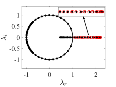
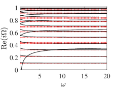
Figure 1: (Color online) The left panel presents the spectrum of a(n unstable) time-periodic solution with $\omega=8$ (filled black circles). Note that the theoretically predicted unstable modes via Eq. (10) are shown with red open circles therein. The right panel demonstrates a comparison between the Floquet exponents $\textrm{Re}(i\Omega)$ of time-periodic solutions (solid black lines) and the ones of the MI analysis (dashed-dotted red lines) of Eq. (10) over $\omega$. Note that both panels correspond to the case with $g=1$ (as well as $C=1$ and $q=1/\sqrt{2}$).

The availability of the exact solution (4) for the case with $g=1$, i.e., the AL limit allows us to not only benchmark our numerical methods but also to compute the Floquet multipliers directly from Eq. (13). Hereafter, we consider a lattice with $N=100$ sites and set $C=1$ and $q=1/\sqrt{2}$ in Eqs. (6) and (12) (all of our numerical results discussed in this section were obtained for these choices). At first, we compute the Floquet multipliers from Eq. (13) (for $g=1$) by using the initial-value-problem (IVP) solver DOP853 Hairer with (relative and absolute) tolerances $10^{-11}$. Although a non-stiff and explicit IVP solver, DOP853 can perform a time step-size adaptation (to satisfy the user-specified tolerance criteria) for stiff regions by reducing the time step-size. Indicatively, Fig. 1 summarizes our findings on the Floquet multipliers for the exact solution (4). The left panel of the figure presents the Floquet multipliers of the exact time-periodic solution with $\omega=8$ (filled black circles) together with the theoretically predicted unstable modes from Eq. (10) via Eq. (14) (open red circles). As far as the KM breather is concerned, the presence of Floquet multipliers with $|\lambda|>1$ render the solution unstable. In addition, it is evident from this panel that a subset of the unstable modes of the KM breather coincides with those of the modulationally unstable background. However, there exist other unstable eigenmodes that deviate from the latter due to the presence of the localized solution perturbing the modes of the background. This is natural to expect given the modulational instability of the background (analyzed in the previous section) on top of which the periodic solution “lives”. The right panel of Fig. 1 complements our analysis of the exact KM breather and demonstrates the dependence of its unstable Floquet exponents $\textrm{Re}(i\Omega)$ on $\omega$ (solid black line) together with the respective results of the MI analysis (dashed-dotted red line). It can be discerned from this panel that the Floquet exponents of the KM breather approach the asymptotic values theoretically predicted by Eq. (10).

We now wish to explore the existence and stability of time-periodic solutions over the relevant parameter space by going beyond the well-defined and analytically tractable case of the integrable limit of $g=1$. We thus vary the parameter $g$ (which is used as our bifurcation parameter) by employing a pseudo-arclength continuation algorithm doedel_I ; ps_method , and consider different fixed values of the period $T$. It should be noted that the pseudo-arclength continuation algorithm is capable of passing through turning points (where the Jacobian of the system of equations is singular and thus non-invertible) and tracing (connected) branches of solutions. The numerical results reported in this work were obtained by using a fixed and relatively small arclength step-size of $10^{-2}$ in order to prevent the predictor-corrector step from converging to a solution of a nearby branch. As per the direct numerical simulations reported below, we use again the DOP853 Hairer method for advancing Eq. (1) forward in time (and with the same tolerance criteria as before).

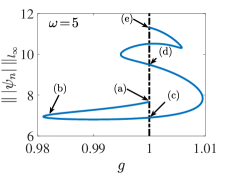
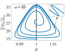
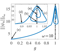
Figure 2: (Color online) The $l_{\infty}$-norm of $|\psi_{n}|$ as a function of $g$ corresponding to time-periodic solutions for values of $\omega=5$, $\omega=25$ and $\omega=10$, respectively. The labels (a)-(e) in the left and right panels are associated with Figs. 3 and 4 that follow.

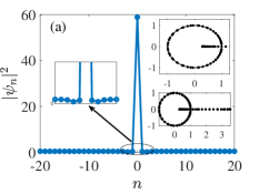
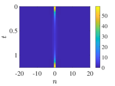
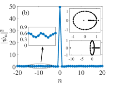
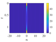
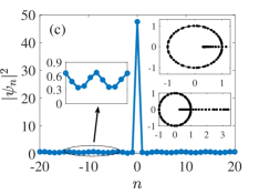
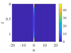
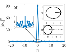
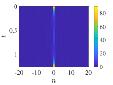
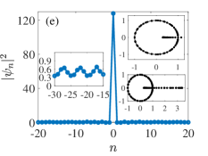
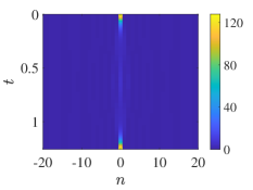
Figure 3: (Color online) Numerical results on time-periodic solutions of the Salerno model (3) for $\omega=5$ associated with the bifurcation curve of the left panel of Fig. 2 (see, the labels therein). The left column corresponds to the spatial distribution of $|\psi_{n}|^{2}$ for values of (a), (c)-(e) $g=1$ and (b) $g=0.982$, respectively. The insets shown on the left and right of each panel provide close-ups of the profiles as well as Floquet spectra. The right column presents the spatio-temporal evolution of $|\psi_{n}|^{2}$ of the profiles shown in the left column for one period ($T=2\pi/5$).

Figure 2 summarizes our results on the existence of of time-periodic solutions to the Salerno model [cf. Eq. (1)]. In particular, we demonstrate the dependence of $\textrm{max}\left(|\psi|\right)$ on $g$ for $\omega=5$, $\omega=25$, and $\omega=10$ in the left, middle, and right panels, respectively. Note that the labels (a)-(e) in the left and right panels are connected to Figs. 3 and 4, respectively. Based on the panels of Fig. 2, a cascade of turning points is clearly evident although all of them suggest an intriguing finding that we discuss now. We consider first the left panel of the figure corresponding to $\omega=5$. Starting from $g=1$, the time-periodic solution departs from the integrable limit (i.e., the AL limit), heading to smaller values of $g$ until it reaches a turning point at $g\approx 0.981$ upon which it comes back to $g=1$, i.e., the AL limit, and then follows a “snake” pattern with several crossings of the AL limit. It should be noted that we stopped our continuation algorithm at $g=1$ (the terminal solution is labeled by (e) therein). Based on our additional numerical investigations, this is en route to multiple additional crossings of $g=1$ (results are not shown). The labels of the left panel are connected with the prototypical configurations for this case in Fig. 3. In particular, its left column presents the spatial distribution of the densities of the time-periodic solutions, i.e., $|\psi_{n}|^{2}$ for values of $g=1$ (panels (a), (c)-(e)), and $g=0.982$ (panel (b)), respectively. The insets therein correspond to the associated Floquet multipliers which themselves suggest that all computed solutions are highly unstable with a dominant unstable mode of the order of $\lambda_{r}\sim\mathcal{O}(1)$. Again, this can be naturally expected on the basis of the instability of the background. The striking feature of the solutions presented in panels (b)-(e) is the formation of an oscillatory background (of small amplitude) in contrast with the KM breather of panel (a) where the localized wave sits atop a constant background. Such profiles featuring small in-amplitude wave trains are strongly reminiscent of nanoptera, and to the best of our knowledge are first reported for the Salerno model in the present work (see, also the recent works of mason_toda ; peli_nano for Toda lattices and the DNLS with saturation). The other striking feature of our findings is that the KM breather (4) of the AL model ($g=1$) seems not to be the only solution at that limit, as this has already been evident in panels (b)-(e) of Fig. 3. Although the investigation of those extra solutions by using integrable systems techniques is of fundamental importance, it is beyond the scope of our present work. We summarize our results in this case by presenting the respective spatio-temporal dynamics in the right panel of Fig. 3. In particular, contour plots of the spatio-temporal evolution of the density of time-periodic solutions are shown for one period ($T=2\pi/5$ in this case). Though the solutions remain robust for one period, thus validating our numerical approach for identifying them (via fixed-point iterations), we observed the emergence of the instability which happens at later times (results not shown) leading to a breakdown of the localized waveform.

Similarly, the middle panel of Fig. 2 corresponds to the case of $\omega=25$. It presents a type of spiral structure around the KM solution that eventually leads to a progressively more dense loop structure that keeps repeating itself in the course of the pseudo-arclength continuation. See also the inset therein which suggests that complex structures may arise also at a fine scale within the bifurcation diagram. The identified periodic states bear similar features as before, including progressively more pronounced (along the relevant branches) tails in the relevant waveforms. Furthermore, in line with earlier (MI-based and computational) findings and general expectations, the solutions are generically found to be unstable, due to the instability of their respective background.

It is perhaps important to highlight two pervading features regarding the nature of our results (both the ones above, as well as the ones that will follow). The first one is that to the best of our knowledge the results above (and below) constitute the first definitive identification of rogue-like patterns in discrete (nonlinear dynamical lattice) systems beyond the extremely important, yet practically limited realm of integrable systems. Secondly, our findings are not solely of interest to non-integrable dispersive system practitioners, but they are also a motivation for further integrable system investigations. The panel (b) of Fig. 3, for example, suggests the existence of KM-type solutions on top of a stationary nanopteronic background which is time-independent in the spirit of recent works of peli1 ; peli2 in corresponding continuum limit problems. These are states that we believe are eminently relevant to explore in an analytical form within the framework of integrable systems (although this is outside the scope of the present study).

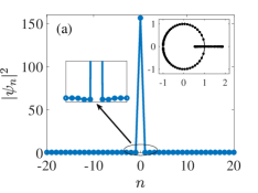
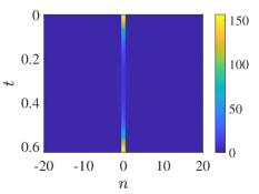
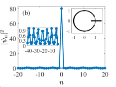
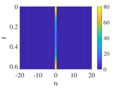
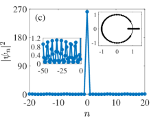
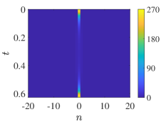
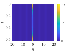
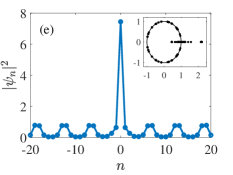
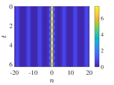
Figure 4: (Color online) Same as Fig. 3 but for the case of $\omega=10$ associated with the right panel of Fig. 2. Again, the left and right columns correspond to the spatial distribution of $|\psi_{n}|^{2}$ and its spatio-temporal evolution, respectively. The integration was performed over one period for (a)-(d) and over $10$ periods for panel (e), respectively. The insets shown on the left and right of each panel provide close-ups of the profiles as well as Floquet spectra. Panels (a)-(c) correspond to $g=1$ whereas the ones of (d) and (e) to $g=0.9$ and $g=0$ (DNLS case), respectively.

We conclude this section of our findings by going through the right panel of Fig. 2 and the associated results shown in Fig. 4 corresponding to the case of $\omega=25$. Based on the former, we observe again a cascade of crossings happening at the AL limit (see, the inset therein), however here the bifurcation curve starts heading towards smaller values of $g$ until it reaches $g=0$, i.e., the DNLS limit. Notice how this appears to be an intermediate case between the less ordered and more expanded diagrams of small $\omega$ and the more ordered and confined diagram of $\omega=25$. The profiles shown in panels (a)-(c) in Fig. 4 correspond to values of $g=1$ whereas the ones of (d) and (e) to $g=0.9$ and $g=0$, respectively. Again, a common finding is that all time-periodic solutions identified in this work feature an oscillatory background as soon as we depart from the integrable limit (see, the left insets in the left column of Fig. 4) as well as they are unstable (see, the right insets therein). This effect is even more pronounced for the case with $g=0$ as is shown in panel (e) of the figure. To the best of our knowledge, such time-periodic solutions of DNLS on a background have not appeared in the literature so far; indeed we are only aware of such effectively quasi-periodic solutions of the model on top of a vanishing background per the work of johaub . This solution is also unstable as is evident in the Floquet spectrum shown in the inset of the panel, although it remains robust over many periods of time integration. Indeed, the right panel therein demonstrates the spatio-temporal evolution of the density again over $10$ periods where $|\psi_{0}(t)|^{2}$ breathes over time. It should also be noted that the oscillatory background is rather visible in this case (as well as the one of panels (b) and (d)) but again it remains steady over the time evolution, i.e., corresponding to a definitive nanopteronic state in this setting.

IV Conclusions and Future Challenges

In this work, we made an attempt to explore the existence, stability and dynamics of time-periodic solutions of the Salerno model. This was with a three-fold scope in mind: firstly, to establish that relevant solutions such as the KM are not unique or particular to the integrable limit, but can be continued to generic non-integrable values of the homotopic parameter $g$. Secondly, we wished to explore whether additional intriguing solutions could arise in the integrable model, a feature that was brought forth from our pseudo-arclength continuation results for periodic orbits. Lastly, we intended to examine whether some of the relevant solutions could be continued to the DNLS limit of $g=0$; here, we found that for suitable choice of the breather frequency indeed that was also possible. Upon employing fixed-point methods, we identified the pertinent waveforms using Newton’s method (for periodic orbits) and their stability was inferred by performing a Floquet analysis. The use of pseudo-arclength continuation allowed us to perform a parametric continuation over the homotopy parameter $g$ and this proved to be crucial in unraveling the complexity of the possible solutions in the Salerno model. Additionally for the integrable limit of $g=1$ we identified multiple time-periodic solutions that sit atop of an oscillatory background being strongly reminiscent of nanoptera. Another striking finding of our work was the time-periodic solution which was identified at the DNLS limit, i.e., $g=0$. To the best of our knowledge, such a waveform for the DNLS (on top of a non-vanishing background) was not previously reported.

Based on the above findings and computational techniques that we have developed in this work, there are clearly many directions for future studies. At the AL limit, a potential analysis of the Zhakarov-Shabat problem for the nanopteronic solutions reported in Section III will be of paramount importance in order to derive them in possibly closed form (analogously to their identification in continuum problems peli1 ; peli2 ). On the other hand, it is worth investigating the $g=0$ solution reported in the present work, and in particular to study the configuration space of solutions as a function of $\omega$ in this case. This will pave the way towards potentially identifying Peregrine-like entities for the DNLS as time-periodic solutions at the limit $T\to\infty$ ($\omega\gg 1$). Another important path to explore is the continuation of the present time-periodic solutions as the distance between adjacent sites decreases, thus approaching the continuum limit when $C=1/h^{2}$ increases. This way, we will be able to connect our findings with the results for the (focusing) NLS. A subset of the above computational studies can be carried out quite efficiently with the use of state-of-the-art bifurcation packages such as AUTO auto and COCO coco which additionally allow branch switching, among other features. Such directions are presently under consideration and will be reported in future publications.

- (1) M. Onorato, S. Residori, U. Bortolozzo, A. Montina, and F. T. Arecchi, Phys. Rep. 528, 47 (2013).
- (2) P. T. S. DeVore, D. R. Solli, D. Borlaug, C. Ropers, and B. Jalali, J. Opt. 15, 064001 (2013).
- (3) Z. Yan, J. Phys. Conf. Ser. 400, 012084 (2012).
- (4) N. Akhmediev et al., J. Opt. 18, 063001 (2016).
- (5) S. Chen, F. Baronio, J. M. Soto-Crespo, P. Grelu, and D. Mihalache, J. Phys. A: Math. Theor. 50, 463001 (2017).
- (6) D. Mihalache, Rom. Rep. Phys. 69, 403 (2017).
- (7) B. A. Malomed and D. Mihalache, Rom. J. Phys. 64, 106 (2019).
- (8) N. Akhmediev, A. Ankiewicz, and M. Taki, Phys. Lett. A 373, 675 (2009).
- (9) E. Pelinovsky and C. Kharif (eds.), Extreme Ocean Waves, Springer-Verlag (New York, 2008).
- (10) C. Kharif, E. Pelinovsky, and A. Slunyaev, Rogue Waves in the Ocean, Springer-Verlag (New York, 2009).
- (11) A. R. Osborne, Nonlinear Ocean Waves and the Inverse Scattering Transform, Academic Press (Amsterdam, 2010).
- (12) M. Onorato, S. Residori, and F. Baronio, Rogue and Shock Waves in Nonlinear Dispersive Media, Springer-Verlag (Heidelberg, 2016).
- (13) A. N. Ganshin, V. B. Efimov, G. V. Kolmakov, L. P. Mezhov-Deglin, and P. V. E. McClintock, Phys. Rev. Lett. 101, 065303 (2008).
- (14) H. Bailung, S. K. Sharma, and Y. Nakamura, Phys. Rev. Lett. 107, 255005 (2011).
- (15) D. R. Solli, C. Ropers, P. Koonath, and B. Jalali, Nature 450, 1054 (2007).
- (16) B. Kibler, J. Fatome, C. Finot, G. Millot, F. Dias, G. Genty, N. Akhmediev, and J. M. Dudley, Nature Phys. 6, 790 (2010) .
- (17) B. Kibler, J. Fatome, C. Finot, G. Millot, G. Genty, B. Wetzel, N. Akhmediev, F. Dias, and J. M. Dudley, Sci. Rep. 2, 463 (2012).
- (18) J. M. Dudley, F. Dias, M. Erkintalo, and G. Genty, Nat. Photon. 8, 755 (2014).
- (19) B. Frisquet, B. Kibler, P. Morin, F. Baronio, M. Conforti, G. Millon, and S. Wabnitz, Sci. Rep. 6, 20785 (2016).
- (20) C. Lecaplain, Ph. Grelu, J. M. Soto-Crespo, and N. Akhmediev, Phys. Rev. Lett. 108, 233901 (2012).
- (21) G. Genty, C. M. de Sterke, O. Bang, F. Dias, N. Akhmediev, and J. M. Dudley, Phys. Lett. A 374, 989 (2010).
- (22) A. Chabchoub, N. P. Hoffmann, and N. Akhmediev, Phys. Rev. Lett. 106, 204502 (2011).
- (23) A. Chabchoub, N. Hoffmann, M. Onorato, and N. Akhmediev, Phys. Rev. X 2, 011015 (2012).
- (24) A. Chabchoub and M. Fink, Phys. Rev. Lett. 112, 124101 (2014).
- (25) J.N. Steer, A.G.L. Borthwick, M. Onorato, A. Chabchoub, and T.S. van den Bremer, Phys. Rev. Lett. 123, 184501 (2019).
- (26) M.J. Ablowitz and J.F. Ladik, J. Math. Phys. 16, 598 (1975).
- (27) M.J. Ablowitz and J.F. Ladik, J. Math. Phys. 17, 1011 (1976).
- (28) D. H. Peregrine, J. Austral. Math. Soc. B 25, 16 (1983).
- (29) E. A. Kuznetsov, Sov. Phys.-Dokl. 22, 507 (1977).
- (30) Ya. C. Ma, Stud. Appl. Math. 60, 43 (1979).
- (31) N. N. Akhmediev, V. M. Eleonskii, and N. E. Kulagin, Theor. Math. Phys. 72, 809 (1987).
- (32) A. Ankiewicz, N. Akhmediev, and J. M. Soto-Crespo, Phys. Rev. E 82, 026602 (2010).
- (33) Y. Ohta and J. Yang, J. Phys. A 47, 255201 (2014).
- (34) P. G. Kevrekidis, The discrete nonlinear Schrödinger equation: Mathematical analysis, Numerical Computations and Physical Perspectives, (Springer-Verlag, Heidelberg, 2009).
- (35) A. Maluckov, Lj. Hadzievski, N. Lazarides, and G. P. Tsironis, Phys. Rev. E 79, 025601(R) (2009).
- (36) C.B. Ward, P.G. Kevrekidis, and N. Whitaker, Phys. Lett. A 383, 2584 (2019).
- (37) C.B. Ward, P.G. Kevrekidis, T.P. Horikis, and D.J. Frantzeskakis, Phys. Rev. Research 2, 013351 (2020).
- (38) J. Cuevas-Maraver, P. G. Kevrekidis, D. J. Frantzeskakis, N. I. Karachalios, M. Haragus, and G. James, Phys. Rev. E 96, 012202 (2017).
- (39) M. Bertola and A. Tovbis, Comm. Pure Appl. Math. 66, 678 (2013).
- (40) A. Tikan, C. Billet, G. El, A. Tovbis, M. Bertola, T. Sylvestre, F. Gustave, S. Randoux, G. Genty, P. Suret, and J.M. Dudley Phys. Rev. Lett. 119, 033901 (2017).
- (41) E.G. Charalampidis, J. Cuevas-Maraver, P.G. Kevrekidis, and D.J. Frantzeskakis, Rom. Rep. Phys. 70, 504 (2018).
- (42) C. Hoffmann, E.G. Charalampidis, D.J. Frantzeskakis, and P.G. Kevrekidis, Phys. Lett. A 382, 3064 (2018).
- (43) M. Salerno, Phys. Rev. A 46, 6856 (1992).
- (44) Y.S. Kivshar and M. Peyrard, Phys. Rev. A 46, 3198 (1992).
- (45) F.Kh. Abdullaev, A. Bouketir, A. Messikh, and B.A. Umarov, Physica D 232, 54 (2007).
- (46) F.II Ndzana and A. Mohamadou, Chaos 27, 073118 (2017).
- (47) E. Hairer, S.P. Nørsett and G. Wanner, Solving ordinary differential equations I (Springer-Verlag, Berlin, 1993).
- (48) A.H. Nayfeh and B. Balachandran, Applied Nonlinear Dynamics: Analytical, Computational and Experimental Methods (Wiley Series in Nonlinear Science, 1995).
- (49) E. Doedel, H.B. Keller and J.P. Kernévez, Internat. J. Bifur. and Chaos, 01, 493-520 (1991).
- (50) C.J. Lustri and M.A. Porter, SIAM J. Appl. Dyn. Sys. 17, 1182 (2018).
- (51) G.L. Afimov, A.S. Korobeinikov, C.J. Lustri, and D.E. Pelinovsky, Nonlinearity 32, 3445 (2019).
- (52) J. Chen, D.E. Pelinovsky, R.E. White, arXiv:1905.11638.
- (53) J. Chen, D.E. Pelinovsky, J. Nonlinear Sci. 29, 2797 (2019).
- (54) M. Johansson and S. Aubry, Nonlinearity 10, 1151 (1997).
- (55) E. Doedel. AUTO. http://indy.cs.concordia.ca/auto/
- (56) H. Dankowicz and F. Schidler. COCO. https://sourceforge.net/projects/cocotools