Optimal error estimates for Legendre expansions of singular functions with fractional derivatives of bounded variation

Abstract.

We present a new fractional Taylor formula for singular functions whose Caputo fractional derivatives are of bounded variation. It bridges and “interpolates” the usual Taylor formulas with two consecutive integer orders. This enables us to obtain an analogous formula for the Legendre expansion coefficient of this type of singular functions, and further derive the optimal (weighted) $L^{\infty}$-estimates and $L^{2}$-estimates of the Legendre polynomial approximations. This set of results can enrich the existing theory for $p$ and $hp$ methods for singular problems, and answer some open questions posed in some recent literature.

1. Introduction

Among the vast family of orthogonal polynomials in the name of German mathematician Carl Gustav Jacob Jacobi (1804-1851)– Jacobi polynomials, the Chebyshev and Legendre polynomials are perhaps the most widely used in numerical analysis (particularly, in spectral methods). Historically, the former has been advocated and promoted to a prevailing “Chebyshev faith”, which asserts that the Chebyshev polynomials are better than any other set of Jacobi polynomials (cf. [Rivlin1969JAT-An, Fox1972Book, Mason2003Book]). After all, (i) the Chebyshev approximation is optimum in the maximum norm; (ii) the Chebyshev polynomials: $T_{n}(x)=\cos(n\,\arccos x))$ and related Gauss-quadrature nodes/weights are explicitly known; (iii) more importantly, they enjoy the fast Fourier transform (FFT) among others. In fact, Boyd and Pestschek [Boyd2014JSC] provided a fair comparison with evidences to show that Legendre and other Jacobi polynomials can win in several exceptional situations. For example, the “spectral elements” [Patera1984JCP-Spectral] were initially Chebyshev-based, but shortly swapped to the Legendre polynomials for at least two reasons: the unpleasant weight function: $1/\sqrt{1-x^{2}}$ brings about troublesome extra terms in the use of integration by parts; and FFT is overkill for low polynomial degree. As such, spectral elements using Legendre polynomials are predominant. On the other hand, it is noteworthy that in a single domain spectral method, the use of compact combination of Legendre polynomials as basis functions [Shen1994SISC], developed into the generalized Jacobi polynomials/functions [24, Guo2009ANM, Chen2016MC], led to optimal spectral algorithms for boundary value problems.

The study of Legendre approximation to singular functions is a subject of fundamental importance in the theory and applications of $hp$ finite element methods. We refer to the seminal series of papers by Gui and Babuška [19, 20, 21] and many other developments in e.g., [37, 7, 8]. In particular, the very recent work of Babuška and Hakula [10] provided a review of known/unknown results and posed a few open questions on the pointwise error estimates of Legendre expansion of a typical singular function discussed in [19]:

$$u(x)=(x-\theta)^{\mu}_{+}=\begin{cases}0,&-1<x\leq\theta,\\[2.0pt] (x-\theta)^{\mu},&\theta<x<1,\end{cases}\quad|\theta|\leq 1,\;\;\;\mu>-1.$$ (1.1)

One significant development along this line is the $hp$ approximation theory in the framework of Jacobi-weighted Besov spaces [7, 8, 9, 22]. Such Besov spaces are defined through space interpolation of Jacobi-weighted Sobolev spaces with integer regularity indices using the $K$-method. It is important to point out that the non-uniformly Jacobi-weighted Sobolev spaces has been employed in spectral approximation theory [18, 37, 25, 24, 38].

1.1. Related works

Different from the Sobolev-Besov framework, Trefethen [40, 41] characterised the regularity of singular functions by using the space of absolute continuity and bounded variation (AC-BV), in the study of Chebyshev expansions of such functions. One motivative example therein is $u(x)=|x|$ in $\Omega=(-1,1)$ which has the regularity: $u,u^{\prime}\in{\rm AC}(\bar{\Omega})$ and $u^{\prime\prime}\in{\rm BV}(\bar{\Omega})$ (where the integration of the norm is in the Riemann-Stieltjes (RS) sense). As a result, the maximum error of its Chebyshev expansion can attain optimal order (but can only be suboptimal in a usual Sobolev framework). There have been many follow-up works on the improved error estimates of Chebyshev approximation or more general Jacobi polynomial approximation under this AC-BV framework (see, e.g., [33, 43, 42, 46]). However, the regularity index and the involved derivatives are of integer order, so it is not suitable to best characterise the regularity of many singular functions, e.g., (1.1) and $u(x)=|x|^{\mu}$ with non-integer $\mu.$ In other words, if one naively applies the estimates, then the loss of order might occur. Nevertheless, the solutions of many singular problems (in irregular domains or with singular coefficients/operators among others) typically exhibit this kind of singularities.

To fill this gap, we introduced for the first time in [32] certain fractional Sobolev-type spaces and derived optimal Chebyshev polynomial approximation to functions with interior and endpoint singularities within this new framework. This study also inspired the discovery of generalised Gegenbauer functions of fractional degree, as an analysis tool and a class of special functions with rich properties [31].

1.2. Our contributions

Undoubtedly, the Taylor formula plays a foundational role in numerical analysis and algorithm development. We present a new fractional Taylor formula for AC-BV functions with fractional regularity index (see Theorem 4.1) that “interpolates” and seamlessly bridges the Taylor formulas of two consecutive integer orders. From this tool, we can derive an analogous formula for the Legendre expansion coefficient of the same class of functions, which turns out the cornerstone of all the analysis. Then we obtain a set of optimal Legendre approximation results in $L^{\infty}$- and $L^{2}$-norms for functions with both interior and endpoint singularities. We highlight that the use of function space involving fractional integrals/derivatives to characterise regularity follows that in [32], but we further refine this framework by introducing the Caputo derivative. When the fractional regularity index takes integer value, it reduces to the AC-BV space in Trefethen [40, 41] (with adaption to the Legendre approximation). We point out that the argument for the Legendre approximation herein is different from that for the Chebyshev approximation in [32]. It is also noteworthy that Babuška and Hakula [10] discussed the point-wise error estimates of the Legendre expansion for the specific function (1.1) (which is also the subject of [19]) including known and unknown results. In fact, it appears necessary to study the point-wise error in the Legendre or other Jacobi cases. For example, the estimating the $L^{\infty}$-error like the Chebyshev expansion can only lead to suboptimal results for functions with the interior singularity, e.g., $u(x)=|x|,$ as a loss of half order occurs. It was observed numerically, but how to obtain optimal estimate appears open (see, e.g., [42]). Here, we shall provide an answer to this, and also to some conjectures in [10]. We remark that we aim at deriving sharp and optimal estimates valid for all polynomial orders. According to [10], in most applications the polynomial orders are relatively small compared to those in the asymptotic range, while the existing theory does not address the behaviour of the pre-asymptotic error. As a result, our arguments and results are different from those in [46], where some asymptotic formulas were employed to derive Jacobi approximation of specific singular functions for large polynomial orders. As a final remark, this paper will be largely devoted to the $L^{\infty}$- and $L^{2}$-estimates of the finite Legendre expansions, which lay the groundwork for establishing the approximation theory of other orthogonal projections, interpolations and quadrature for singular functions. Indeed, these results can enrich the theoretical foundation of $p$ and $hp$ methods (cf. [18, 37, 11, 16, 26, 38]). In a nutshell, the present study together with [31, 32] is far from being the last word on this subject.

The rest of the paper is organised as follows. In section 4, we derive the fractional Taylor formula for the AC-BV functions and present some preliminaries to pave the way for all forthcoming discussions. In section 5, we obtain the main results on Legendre approximation of functions with interior singularities and extend the tools to study the endpoint singularities in section 6.

In fact, we can interpret the functions in those spaces being of AC_m-BV${}_{\!s,\theta}$-regularity for some $s\in(0,1)$ and given $\theta\in(-1,1)$ corresponding to the location of the interior singularity (cf. Definition LABEL:functionA). For example, the regularity indices $m,s$ of (1.1) are $m+s=\alpha+1$ with $m=[\alpha+1].$ The “fractional regularity” is characterised by the Riemann-Liouville (RL) fractional integration of $u^{(m)}$ at $\theta$ of order $1-s$, which can capture the additional regularity with the index “$s$”, as the RL fractional integration can increase the regularity of such singular functions. When $s=1,$ it reduces to the space in [40, 41]. When $\theta=\pm 1,$ it leads to the framework for endpoint singularities (cf. Definition 6.1). We point out that the analytical study of Legendre expansion of (1.1) in Gui and Babuška [19] actually sheds light on our analysis tools to derive optimal error estimates. More precisely, for $\theta\in(-1,1),$ the following exact formula for the Legendre coefficient was derived in [19]:

$$\hat{u}_{n}^{L}=\frac{2n+1}{2}\int_{-1}^{1}(x-\theta)^{\alpha}_{+}\,P_{n}(x)\,{\rm d}x=C_{n}^{(\alpha)}(1-\theta)^{\alpha+1}P_{n}^{(\alpha+1,-\alpha-1)}(\theta),$$ (1.2)

where $C_{n}^{(\alpha)}$ is an explicit constant. The analysis therein heavily relied on the formula (cf. [Gradshteyn1975Book, p. 833]): for $\mu>0$ and $\gamma\in(0,1),$

$$\int_{0}^{1}(1-y)^{\mu-1}P_{n}(1-\gamma y)\,{\rm d}y=\frac{\Gamma(\mu)\,n!}{\Gamma(\mu+n+1)}P_{n}^{(\mu,-\mu)}(1-\gamma),$$ (1.3)

where $P_{n}^{(\mu,-\mu)}(x)$ is the (generalised) Jacobi polynomial with one parameter possibly $<-1.$ Interestingly, with the substitution: $t=1-\gamma y$ and $x=1-\gamma,$ the formula (1.3) turns out to be

$$\frac{1}{\Gamma(\mu)}\int_{x}^{1}\frac{P_{n}(t)}{(t-x)^{1-\mu}}\,{\rm d}t=\frac{n!}{\Gamma(\mu+n+1)}{(1-x)^{\mu}P_{n}^{(\mu,-\mu)}(x)},$$ (1.4)

where the left-hand side is the RL fractional integral of $P_{n}(x),$ i.e., $I_{1-}^{\mu}P_{n}(x)$ (cf. (4.16)).

The above snapshots clearly indicate that the RL fractional calculus and (generalised) Jacobi polynomials with the parameters in non-classical ranges played an important part in the analysis of [19]. It is not a coincidence that these threads can be found in the optimal $L^{\infty}$-error estimates of Chebyshev approximation [32]. In fact, they can be seen more evidently in this context, as the generalised Gegenbauer functions of fractional degree (GGF-Fs) [32, 31] (counterpart of generalised Jacobi polynomials) and the RL fractional integration by parts are indispensable for the derivation of the exact formula for the Legendre expansion coefficient (see Theorems 5.2 and 6.2). As already mentioned, the analysis in [19, 20, 21] had deep impact upon the $hp$-approximation theory in Jacobi-weighted Besov spaces [7, 8, 9, 22]. To some extent, we however drive this to a different path with the aid of tools from RL fractional calculus, leading to the space of functions, e.g., with AC_m-BV${}_{\!s,\theta}$-regularity that can seamlessly bridge the gaps in [40, 41].

We summarise and highlight that this work can stand out from many existing works mentioned earlier, in particular, the very recent papers [42, 32, 10, 46] attributed to the following features.

• Different from [42, 46] and the related works cited therein, we consider the Legendre approximation of singular functions with AC_m-BV${}_{\!s,\theta}$-regularity, rather than the usual AC_m-BV-regularity [40, 41]. Most existing results corresponding to the special case with $s=1.$ Moreover, our argument leads to sharper results as we shall illustrate in the text.

• We aim at deriving sharp and optimal estimates valid for all polynomial orders. As pointed out in [10], in most applications the polynomial orders are relatively small compared to those in the asymptotic range, while the existing theory does not address the behaviour of the pre-asymptotic error. As a result, our arguments and results are different from those in [46], where some asymptotic formulas were employed to derive Jacobi approximation of specific singular functions for large polynomial orders.

• Some results in [32, 31] pave the way for this study, but much more delicate analysis and additional tools are needed for the Legendre approximations. In fact, it is believed that the Legendre case has a more extendability of the arguments and results to the other Jacobi cases.

It is known that polynomial approximation theory is of fundamental importance in numerical analysis and algorithm development of many computational methods, e.g., $p$/$hp$ finite elements or spectral/spectral-element methods (see, e.g., [18, 37, 11, 16, 26, 38] and references therein). Typically, the documented approximation results take the form

$$\|Q_{N}u-u\|_{\mathcal{S}_{\rm l}}\leq cN^{-\sigma}|u|_{\mathcal{B}_{\rm r}},\quad\sigma\geq 0,$$ (1.5)

where $Q_{N}$ is an orthogonal projection (or interpolation operator) upon the set of all polynomials of degree at most $N,$ and $c$ is a positive constant independent of $N$ and $u$. In (1.5), ${\mathcal{S}}_{\rm l}$ is a certain Sobolev space, ${\mathcal{B}}_{\rm r}$ is a related Sobolev or Besov space, and $\sigma$ depends on the regularity exponentials of both ${\mathcal{B}}_{\rm r}$ and ${\mathcal{S}}_{\rm l}$. In practice, one would expect (a) the space ${\mathcal{B}}_{\rm r}$ should contain the classes of functions as broad as possible; and (b) the space ${\mathcal{B}}_{\rm r}$ can best characterise their regularity leading to optimal order of convergence. In general, the space ${\mathcal{B}}_{\rm r}$ is of the following types.

• ${\mathcal{B}}_{\rm r}$ is the standard weighted Sobolev space $H^{m}_{\omega}(\Omega)$ with integer $m\geq 0$ and certain weight function $\omega(x)$ on $\Omega=(-1,1)$ (see, e.g., [11, 16, 26]). However, it could not lead to optimal order for functions with endpoint singularities (see, e.g., [11, 25]) or with interior singularities, e.g., $|x|$ (see [40]).

• ${\mathcal{B}}_{\rm r}$ is the non-uniformly Jacobi-weighted Sobolev space (see, e.g., [18, 7, 8, 25, 24, 38]). For example, ${\mathcal{B}}_{\rm r}=H^{m,\beta}(\Omega)$ with integer $m\geq 0$ and $\beta>-1,$ is defined as a closure of $C^{\infty}$-functions endowed with the weighted norm

  $$\|u\|_{H^{m,\beta}(\Omega)}=\bigg{\{}\sum_{k=0}^{m}\int_{-1}^{1}|u^{(k)}(x)|^{2}(1-x^{2})^{\beta+k}dx\bigg{\}}^{1/2}.$$ (1.6)

  Compared with the standard Sobolev space in (i), such spaces can better describe the endpoint singularities, but still produce suboptimal estimates for $(1+x)^{\alpha}$-type singular functions with non-integer $\alpha>0$ (cf. [Castillo2002MC, P. 474]). Indeed, for the Chebyshev approximation, we find that $u=(1+x)^{\alpha}\in{H^{m,-1/2}(\Omega)}$ with integer $m<2\alpha+1/2,$ and

  $$\|\pi_{N}^{C}u-u\|_{L^{2}_{\omega}(\Omega)}\leq cN^{-m}|u|_{H^{m,-1/2}(\Omega)},$$ (1.7)

  where $\pi_{N}^{C}u$ is the $L^{2}_{\omega}$-orthogonal projection of $u$ (with $\omega=(1-x^{2})^{-1/2}$). However, the expected optimal order is $O(N^{-2\alpha-1/2}),$ so the loss of an order of the fractional part of $2\alpha+1/2$ or one order (when $2\alpha=k+1/2$ with integer $k\geq 0$), is inevitable under this framework. This is due to the space $H^{m,\beta}(\Omega)$ is only defined for integer $m\geq 0.$

• In a series of works [7, 8, 9], Babuška and Guo introduced the Jacobi-weighted Besov space defined by space interpolation based on the so-called K-method. One commonly used Besov space for $(1+x)^{\alpha}$-type corner singularities is ${\mathcal{B}}^{s,\beta}_{2,2}(\Omega)=(H^{l,\beta}(\Omega),H^{m,\beta}(\Omega))_{\vartheta,2}$ with integers $l<m$ and $s=(1-\vartheta)l+\vartheta m,\vartheta\in(0,1),$ equipped with the norm

  $$\begin{split}&\|u\|_{{\mathcal{B}}^{s,\beta}_{2,2}(\Omega)}=\bigg{(}\int_{0}^{\infty}t^{-2\vartheta}|K(t,u)|^{2}\frac{dt}{t}\bigg{)}^{1/2}\!,\quad{\rm where}\\ &K(t,u)=\inf_{u=v+w}\big{(}\|v\|_{H^{l,\beta}(\Omega)}+t\|w\|_{H^{m,\beta}(\Omega)}\big{)}.\end{split}$$ (1.8)

  However, to deal with $(1+x)^{\alpha}\log^{\nu}(1+x)$-type corner singularities, Babuška and Guo had to further modify the K-method by incorporating a log-factor into the norm.

The aforementioned framework might lead to suboptimal estimates for functions with interior singularities. For example, we consider $u(x)=|x|$ for $x\in(-1,1).$ Note that $u^{\prime}(x)=2H(x)-1$ and $u^{\prime\prime}(x)=2\delta(x)$ (where $H,\delta$ are respectively the Heaviside function and the Dirac delta function). Since $u^{\prime\prime}\not\in L^{2}(\Omega)$, the Chebyshev approximation of $|x|$ has a convergence:

$$\|\pi_{N}^{C}u-u\|_{L^{2}_{\omega}(\Omega)}\leq cN^{-1}|u|_{H^{1,-1/2}(\Omega)},$$ (1.9)

but the expected optimal order is $O(N^{-3/2})$ (cf. [40, 41]). In fact, as shown in [40, Thms 4.2-4.3] and [41, Thms 7.1-7.2] (also see Lemma LABEL:trenstha below), one should choose ${\mathcal{B}}_{\rm r}\subseteq{\rm BV}(\bar{\Omega})$ (the space of functions of bounded variation) to achieve optimality (see Section LABEL:sect:existingest, and refer to [40, Xiang2010NM, 41, 33] for more details). Unfortunately, the Sobolev spaces therein were defined through integer-order derivatives, so they could not best characterise the regularity of e.g., $u(x)=|x|^{\alpha}$ with non-integer $\alpha>0.$ In other words, the order of convergence is suboptimal.

In this paper, we intend to introduce a new framework of fractional Sobolev-type spaces that can meet the two requirements (a)-(b) and overcome the deficiencies mentioned above. We focus on the Chebyshev approximation but the analysis techniques are extendable to general Jacobi approximations. Here, we put the emphasises on estimating the decay rate of expansion coefficients for the reason that the errors of spectral expansions in various norms, and the related interpolation and quadratures can be estimated directly from the sums of the coefficients (cf. [40, 33]). The essential ideas and main contributions of this study are summarised as follows.

• We derive the exact representation of the Chebyshev expansion coefficients (see Theorem 5.1) by using the fractional calculus properties of GGF-Fs and fractional integration by parts (under the weakest possible conditions). This allows us to naturally define the fractional Sobolev spaces to characterise the regularity of a large class of singular functions, leading to optimal order of convergence.

• As a by-product, our estimates for the functions in this framework with integer regularity exponential can improve the existing bounds in usual Sobolev spaces (see, e.g., [40, Xiang2010NM, 41, 33]).

• We present some useful analytical formulas on fractional calculus of GGF-Fs, and the Chebyshev expansions of some specific singular functions. Some of them are new or difficult to be derived by other means (cf. [Gui1986NM, Boyd1989AMC, 43]). They are also useful for the design of spectral algorithms.

The paper is organised as follows. In Sections LABEL:sect:gegenbaure-4, we introduce the GGF-Fs, and present their important properties, including the uniform bounds and Riemann-Liouville fractional integral/derivative formulas. We derive the main results in Section LABEL:mainsect:ms, and improve the existing estimates in Sobolev spaces with integer-order derivatives in Section LABEL:sect:existingest. We discuss in Section LABEL:Sect6Analysis the extension of the main results to the analysis of interpolation, quadrature and endpoint singularities.

2. Preliminaries and illustrative examples

2.1. Illustrative examples

For clarity of presentations, we start with the some relatively simple but illustrative examples to motivate the introduction of the analysis tools.

Given $\theta\in[-1,1),$ we consider

$$u(x)=g(x)|x-\theta|^{\alpha},\quad x\in(-1,1),$$ (2.1)

where $g(x)\in C^{\infty}(-1,1).$

More recently, Wang [42] showed that if $f,f^{\prime},\ldots,f^{(m-1)}$ are absolutely continuous, $f^{(m)}$ has a bounded variation and $\int^{1}_{-1}|f^{(m+1)}(x)|(1-x^{2})^{-1/4}dx<\infty$

$$|\hat{u}_{n}^{L}|\leq\frac{2}{\sqrt{\pi(2n-2m-1)}}\frac{\Gamma(n-m+1/2)}{\Gamma(n+1/2)}\int^{1}_{-1}|f^{(m+1)}(x)|(1-x^{2})^{-1/4}dx.$$ (2.2)

The $L^{2}$ orthogonal projection is defined by

$$\pi_{N}^{L}u(x):=\sum_{n=0}^{N}\hat{u}_{n}^{L}\,P_{n}(x).$$

The decay of the

3. Preliminaries

of fractional calculus, related spaces of functions, and with some their properties.

3.1. Fractional calculus and related spaces of functions

4. Fractional integral/derivative formulas of GGF-Fs

In this section, we make necessary preparations for the forthcoming discussions. More precisely, we first introduce several spaces of functions that will be used to characterise the regularity of the class of functions of interest. We then recall the definition of the Riemann-Liouville (RL) fractional integrals, and present a useful RL fractional integration parts formula. Finally, we collect some relevant properties of generalised Gegenbauer functions of fractional degree (GGF-Fs), which were first introduced and studied in [32, 31].

4.1. Spaces of functions

Let $\Omega=(a,b)\subset{\mathbb{R}}$ be a finite open interval. For real $p\in[1,\infty],$ let $L^{p}(\Omega)$ (resp. $W^{m,p}(\Omega)$ with $m\in{\mathbb{N}},$ the set of all positive integers) be the usual $p$-Lebesgue space (resp. Sobolev space), equipped with the norm $\|\cdot\|_{L^{p}(\Omega)}$ (resp. $\|\cdot\|_{W^{m,p}(\Omega)}$), as in Adams [1].

Let $C(\bar{\Omega})$ be the classical space of continuous functions, and ${\rm AC}(\bar{\Omega})$ the space of absolutely continuous functions on $\bar{\Omega}.$ It is known that every absolutely continuous function is uniformly continuous (but the converse is not true), and hence continuous (cf. ​[35, p.​ 483]). It is known that a real function $f(x)\in{\rm AC}(\bar{\Omega})$ if and only if $f(x)\in L^{1}(\Omega)$, $f(x)$ has a derivative $f^{\prime}(x)$ almost everywhere on $[a,b]$ such that $f^{\prime}(x)\in L^{1}(\Omega),$ and $f(x)$ has the integral representation:

$$f(x)=f(a)+\int_{a}^{x}f^{\prime}(t)\,{\rm d}t,\quad\forall\,x\in[a,b],$$ (4.1)

(cf.​ [36, Chap.​ 1] and [30, p.​ 285]).

According to [Leoni2009Book, Ch. 3] (also see [13, P. 206] or [36, Ch. 1]), a real function $f(x)\in{\rm AC}(\bar{\Omega}),$ if for any $\varepsilon>0,$ there exists $\delta>0,$ such that for every finite sequence of disjoint intervals $(a_{k},b_{k})\subset\Omega$ such that $\sum_{k}|b_{k}-a_{k}|<\delta,$ we have $\sum_{k}|f(b_{k})-f(a_{k})|<\varepsilon.$

Recall that (cf. [36, Ch. 1] or [30, P. 285]): a real function $f(x)\in{\rm AC}(\bar{\Omega})$ if and only if $f(x)\in L^{1}(\Omega)$, $f(x)$ has a derivative $f^{\prime}(x)$ almost everywhere on $[a,b]$ such that $f^{\prime}(x)\in L^{1}(\Omega),$ and $f(x)$ has the integral representation:

$$f(x)=f(a)+\int_{a}^{x}f^{\prime}(t)\,dt,\quad\forall x\in[a,b].$$

Let ${\rm BV}(\bar{\Omega})$ be the space of functions of bounded variation on $[a,b].$ We say that a real function $f(x)\in{\rm BV}(\bar{\Omega}),$ if there exists a constant $C>0$ such that

$$V({\mathbb{P}};f):=\sum\limits_{i=0}^{k-1}|f(x_{i+1})-f(x_{i})|\leq C$$

for every finite partition ${\mathbb{P}}=\{x_{0},x_{1},\cdots,x_{k}\}$ (satisfying $x_{i}<x_{i+1}$ for all $0\leq i\leq k-1$) of $[a,b].$ Then the total variation of $f$ on $[a,b]$ is defined as $V_{\bar{\Omega}}[f]:=\sup\{V({\mathbb{P}};f)\},$ where the supreme is taken over all the partitions of $\bar{\Omega}$ (cf. [13, p.​ 207] or [30, Chap.​ X]). An important characterisation of a BV-function is the Jordan decomposition (cf. ​[35, Thm.​ 11.19]): a function is of bounded variation if and only if it can be expressed as the difference of two increasing functions on $[a,b].$ As a result, every function in ${\rm BV}(\bar{\Omega})$ has at most a countable number of discontinuities, which are either jump or removable discontinuities, so it is differentiable almost everywhere. Indeed, according to [6, p.​ 223], if $f\in{\rm AC}(\bar{\Omega}),$ then

$$V_{\bar{\Omega}}[f]=\int_{\Omega}|f^{\prime}(x)|\,{\rm d}x.$$

In fact, we have ${\rm BV}(\bar{\Omega})\subset{\rm AC}(\bar{\Omega})={\rm W}^{1,1}(\Omega)$ in the sense that every $f(x)\in{\rm AC}(\bar{\Omega})$ has an almost everywhere classical derivative $f^{\prime}\in L^{1}(\Omega)$ (cf. (4.1)) and $f^{\prime}(x)$ is the weak derivative of $f(x).$ Conversely, even $f\in W^{1.1}(\Omega),$ modulo a modification on a set of measure zero, is an absolutely continuous function (cf.​ [13, p.​ 206] and [15, p.​ 84; p.​ 96]).

For BV-functions, we can define the Riemann-Stieltjes (RS) integral (cf.​ [30, Chap.​​ X]). A function $f(x)$ is said to be RS($g$)-integrable, if $\int_{\Omega}f{\rm d}g<\infty$ for $g\in{\rm BV}(\bar{\Omega}).$ From [30, Prop.​ 1.3], we have that if $f$ is RS($g$)-integrable, then

$$\Big{|}\int_{\Omega}f(x)\,{\rm d}g(x)\Big{|}\leq\|f\|_{\infty}\,V_{\bar{\Omega}}[f],\quad\int_{\Omega}|{\rm d}g(x)|=V_{\bar{\Omega}}[g],$$ (4.2)

where $\|f\|_{\infty}$ is the $L^{\infty}$-norm of $f$ on $[a,b].$

In the analysis, we shall also use the splitting rule of a RS integral, which is different from the usual integral.

Lemma 4.1 (see Carter and Brunt [17, Thm 6.1.1 & Thm 6.1.6]).

If the interval $\Omega$ is a union of a finite number of pairwise disjoint intervals $\Omega=\Omega_{1}\cup\Omega_{2}\cup\cdots\cup\Omega_{m},$ then

$$\int_{\Omega}f{\rm d}g=\sum_{j=1}^{m}\int_{\Omega_{j}}f{\rm d}g$$

in the sense that if one side exists, then so does the other, and the two are equal. Moreover, for any function $f$ defined at $\theta,$ then

$$\int_{[\theta,\theta]}f{\rm d}g=f(\theta)(g(\theta+)-g(\theta-)).$$

4.2. Formula of fractional integration by parts

Recall the formula of integration by parts involving the Riemann-Stieltjes integrals (cf. ​[28, (1.20)]): if $f,g\in{\rm BV}(\bar{\Omega})$, we have

$$\int_{a}^{b}f(x)\,{\rm d}g(x)=\{f(x)g(x)\}\big{|}_{a^{+}}^{b^{-}}-\int_{a}^{b}g(x)\,{\rm d}f(x),$$ (4.3)

where we denote

$$f(x)\big{|}_{a^{+}}^{b^{-}}=\lim\limits_{x\to b^{-}}f(x)-\lim\limits_{x\to a^{+}}f(x)=f(b-)-f(a+).$$

In particular, if $f,g\in\mathrm{AC}(\bar{\Omega}),$ we have

$$\int_{a}^{b}f(x)g^{\prime}(x)\,{\rm d}x+\int_{a}^{b}f^{\prime}(x)g(x)\,{\rm d}x=\{f(x)g(x)\}\big{|}_{a}^{b}.$$

In what follows, we shall derive a formula of fractional integration parts from (4.3) in a weaker sense than the existing counterparts (cf.​ [36, 12]). For this purpose, we recap on the definition of the Riemann-Liouville fractional integral (cf.​ [36, p.​ 33, p.​ 44]): for any $f\in L^{1}(\Omega),$ the left-sided and right-sided Riemann-Liouville fractional integrals of real order $\rho\geq 0$ are defined by

$$\begin{split}&(I_{a+}^{\rho}f)(x)=\frac{1}{\Gamma(\rho)}\int_{a}^{x}\frac{f(y)}{(x-y)^{1-\rho}}{\rm d}y;\quad(I_{b-}^{\rho}f)(x)=\frac{1}{\Gamma(\rho)}\int_{x}^{b}\frac{f(y)}{(y-x)^{1-\rho}}{\rm d}y,\end{split}$$ (4.4)

for $x\in\Omega,$ where $\Gamma(\cdot)$ is the usual Gamma function. For $\mu\in(k-1,k]$ with $k\in\mathbb{N},$ the left-sided and right-side Caputo fractional derivatives of order $\mu$ are respectively defined by

$$({}^{C}\!D_{a+}^{\mu}f)(x)=(I_{a+}^{k-\mu}f^{(k)})(x);\quad({}^{C}\!D_{b-}^{\mu}f)(x)=(-1)^{k}(I_{b-}^{k-\mu}f^{(k)})(x).$$ (4.5)

The following formula of fractional integration by parts plays an important role in the analysis, which can be derived from (4.3) (see Appendix B).

Lemma 4.2.

Let $\rho\geq 0,f(x)\in L^{1}(\Omega)$ and $g(x)\in{\rm AC}(\bar{\Omega}).$

• If $I_{b-}^{\rho}f(x)\in{\rm BV}(\bar{\Omega}),$ then

  $$\begin{split}\int^{b}_{a}f(x)&\,I_{a+}^{\rho}g^{\prime}(x)\,{\rm d}x=\big{\{}g(x)\,I_{b-}^{\rho}f(x)\big{\}}\big{|}_{a^{+}}^{b^{-}}-\int^{b}_{a}g(x)\,{{\rm d}\big{\{}I_{b-}^{\rho}f(x)\big{\}}}.\end{split}$$ (4.6)

• If $I_{a+}^{\rho}f(x)\in{\rm BV}(\bar{\Omega}),$ then

  $$\begin{split}\int^{b}_{a}f(x)&\,I_{b-}^{\rho}g^{\prime}(x)\,{\rm d}x=\big{\{}g(x)\,I_{a+}^{\rho}f(x)\big{\}}\big{|}_{a^{+}}^{b^{-}}-\int^{b}_{a}g(x)\,{{\rm d}\big{\{}I_{a+}^{\rho}f(x)\big{\}}}.\end{split}$$ (4.7)

Remark 4.1.

If $\rho=0,$ then they reduce (4.3). It is known that the fractional integral can improve the regularity. Indeed, for $0<\rho<1$ and $u\in L^{1}(\Omega),$ we have $I_{a+}^{\rho}u,I_{b-}^{\rho}u\in L^{p}(\Omega)$ with $p\in[1,\rho^{-1})$ (cf.​ [12, Prop.​ 2.1]). ∎

Compared with those in [36, 12], a weaker condition is imposed on $f(x)$ in (4.6)-(4.7), which turns out essential in dealing with the singular functions. Moreover, for such functions, the limit values $\lim_{x\to a^{+}}I_{a+}^{\rho}f(x)$ in (4.6), and $\lim_{x\to b^{-}}I_{b-}^{\rho}f(x)$ in (4.7) might be nonzero, in contrast to a usual integral with $\rho=1.$ For example, for $\rho\in(0,1),$ we have

$$I_{a+}^{1-\rho}\,(x-a)^{\rho-1}=I_{b-}^{1-\rho}\,(b-x)^{\rho-1}=\Gamma(\rho),$$

which follow from the explicit formulas $($cf. [36]$)$: for real $\eta>-1$ and $\rho\geq 0,$

$$I_{a+}^{\rho}(x-a)^{\eta}=\dfrac{\Gamma(\eta+1)}{\Gamma(\eta+\rho+1)}(x-a)^{\eta+\rho};\quad I_{b-}^{\rho}(b-x)^{\eta}=\dfrac{\Gamma(\eta+1)}{\Gamma(\eta+\rho+1)}(b-x)^{\eta+\rho}.$$ (4.8)

In fact, we have the following more general formula, which finds useful in exemplifying some estimates to be presented later. We sketch the derivation in Appendix C.

Proposition 4.1.

Let $f(x)=(x-a)^{\gamma}g(x)$ with real $\gamma>-1$, where $g(x)$ is bounded and Riemann integrable on $[a,a+\delta)$ for some $\delta>0.$ Then for real $\rho>0$, we have

$$\lim_{x\to a^{+}}(I_{a+}^{\rho}\,f)(x)=\begin{cases}0,&{\rm if}\;\;\rho>-\gamma,\\ g(a)\Gamma(\gamma+1),&{\rm if}\;\;\rho=-\gamma,\\ \infty,&{\rm if}\;\;\rho<-\gamma.\end{cases}$$ (4.9)

Let $f(x)=(b-x)^{\gamma}g(x)$, $\gamma>-1$, and $g(x)$ be bounded and Riemann integrable on $(b-\delta,b].$ Then the same result holds for the limit $\lim\limits_{x\to b^{-}}(I_{b-}^{\rho}\,f)(x)$ but with $g(b)$ in place of $g(a).$

4.3. Fractional Taylor formula

Needless to say, the Taylor formula plays a fundamental role in many branches of mathematics. For comparison purpose, we recall this well-known formula: Let $k\geq 1$ be an integer and let $f(x)$ be a real function that is $k$ times differentiable at the point $x=\theta$. Further, let $f^{(k)}(x)$ be absolutely continuous on the closed interval between $\theta$ and $x$. Then we have

$$f(x)=\sum_{j=0}^{k}\frac{f^{(j)}(\theta)}{j!}(x-\theta)^{j}+\int_{\theta}^{x}\frac{f^{(k+1)}(t)}{k!}(x-t)^{k}\,{\rm d}t.$$ (4.10)

Note that since $f^{(k)}(x)$ is an AC-function, $f^{(k+1)}(x)$ exists as an $L^{1}$-function.

As a second building block for the analysis, we derive a fractional Taylor formula from Lemma 4.2 and (4.10).

Theorem 4.1 (Fractional Taylor formula).

Let $\mu\in(k-1,k]$ with $k\in\mathbb{N},$ and let $f(x)$ be a real function that is $(k-1)$times differentiable at the point $x=\theta$.

• If $f^{(k-1)}\in{\rm AC}([\theta,x])$ and ${}^{C}\!D_{\theta+}^{\mu}f\in{\rm BV}([\theta,x]),$ then we have the left-sided fractional Taylor formula

  $$\begin{split}f(x)=\sum_{j=0}^{k-1}\frac{f^{(j)}(\theta)}{j!}(x-\theta)^{j}+\frac{{}^{C}\!D_{\theta+}^{\mu}f(\theta+)}{\Gamma(\mu+1)}{(x-\theta)^{\mu}}+\frac{1}{\Gamma(\mu+1)}\int_{\theta}^{x}(x-t)^{\mu}\,{\rm d}\{{}^{C}\!D_{\theta+}^{\mu}f(t)\}.\end{split}$$ (4.11)

• If $f^{(k-1)}\in{\rm AC}([x,\theta])$ and ${}^{C}\!D_{\theta-}^{\mu}f\in{\rm BV}([x,\theta]),$ then we have the right-sided fractional Taylor formula

  $$\begin{split}f(x)=\sum_{j=0}^{k-1}\frac{f^{(j)}(\theta)}{j!}(x-\theta)^{j}+\frac{{}^{C}\!D_{\theta-}^{\mu}f(\theta-)}{\Gamma(\mu+1)}{(\theta-x)^{\mu}}-\frac{1}{\Gamma(\mu+1)}\int^{\theta}_{x}(t-x)^{\mu}\,{\rm d}\{{}^{C}\!D_{\theta-}^{\mu}f(t)\}.\end{split}$$ (4.12)

Proof.

By (4.10) (with $k\to k-1$), we have

$$\begin{split}f(x)&=\sum_{j=0}^{k-1}\frac{f^{(j)}(\theta)}{j!}(x-\theta)^{j}+\frac{1}{(k-1)!}\int_{\theta}^{x}(x-t)^{k-1}f^{(k)}(t)\,{\rm d}t.\end{split}$$ (4.13)

From (4.8), we find readily that for $x>t,$

$$(x-t)^{k-1}=-\frac{(k-1)!}{\Gamma(\mu+1)}I_{x-}^{k-\mu}\Big{\{}\frac{{\rm d}}{{\rm d}t}(x-t)^{\mu}\Big{\}}.$$

Thus, we can rewrite (4.13) as

$$\begin{split}f(x)&=\sum_{j=0}^{k-1}\frac{f^{(j)}(\theta)}{j!}(x-\theta)^{j}-\frac{1}{\Gamma(\mu+1)}\int_{\theta}^{x}I_{x-}^{k-\mu}\Big{\{}\frac{{\rm d}}{{\rm d}t}(x-t)^{\mu}\Big{\}}f^{(k)}(t)\,{\rm d}t.\end{split}$$ (4.14)

Substituting $a,$ $b,$ $\rho,$ $f$ and $g$ in (4.7) of Lemma 4.2 by $\theta,$ $x,$ $k-\mu$, $f^{(k)}(t)$ and $(x-t)^{\mu},$ respectively, we obtain that for $x>\theta,$

$$\begin{split}\int_{\theta}^{x}I_{x-}^{k-\mu}\Big{\{}\frac{{\rm d}}{{\rm d}t}(x-t)^{\mu}\Big{\}}f^{(k)}(t)\,{\rm d}t&=-{I_{\theta+}^{k-\mu}f^{(k)}(\theta+)}(x-\theta)^{\mu}-\int_{\theta}^{x}(x-t)^{\mu}\,{\rm d}\{{I_{\theta+}^{k-\mu}f^{(k)}(t)}\}\\ &=-{}^{C}\!D_{\theta+}^{\mu}f(\theta+){(x-\theta)^{\mu}}-\int_{\theta}^{x}(x-t)^{\mu}\,{\rm d}\{{}^{C}\!D_{\theta+}^{\mu}f(t)\},\end{split}$$ (4.15)

where in the last step, we used the definition (4.5). Thus, we obtain (4.11) from (4.14)-(4.15) immediately.

The right-sided formula (4.12) can be obtained in a very similar fashion. ∎

Remark 4.2.

When $\mu=k,$ the fractional Taylor formulas (4.11) and (4.12) lead to (4.10). The fractional formula can be viewed as the “interpolation” of the integer-order Taylor formulas with the regularity indexes $k-1$ and $k.$ Apparently, the integer-order Taylor formula (4.10) is exact for all $f\in{\mathcal{P}_{k}}={\rm span}\{(x-\theta)^{j}\,:\,0\leq j\leq k\}.$ In the fractional case, the exactness of (4.11) is for all $f\in{\mathcal{P}_{k-1}}\cup\{(x-\theta)^{\mu}\}$ (i.e., the remainder vanishes). We can verify this readily from (4.5) and the fundamental formula: ${}^{C}\!D_{\theta+}^{\mu}\{(x-\theta)^{\mu}\}=\Gamma({\mu+1}).$ Note that the right-sided formula (4.12) is exact for all $f\in{\mathcal{P}_{k-1}}\cup\{(\theta-x)^{\mu}\}.$ ∎

We remark that there are several versions of fractional Taylor formulas for functions with different regularities. For example, Anastassiou [3, (21)] stated the right-sided fractional Taylor formula: for real $\mu\geq 1,$ let $k=[\mu]$ be its integer part, and assume that $f,f^{\prime},\ldots,f^{(k-1)}\in{\rm AC}([x,\theta]).$ Then

$$f(x)=\sum_{j=0}^{k-1}\frac{f^{(j)}(\theta)}{j!}(x-\theta)^{j}+\frac{1}{\Gamma(\mu)}\int_{x}^{\theta}(t-x)^{\mu-1}\,{}^{C}\!D_{\theta{-}}^{\mu}f(t)\,{\rm d}t.$$

Kolwankar and Gangal [29] presented some local fractional Taylor expansion with a different fractional derivative in the remainder.

Denote the ordinary derivatives by ${\mathcal{D}}=d/dx$ and ${\mathcal{D}}^{k}=d^{k}/dx^{k}$ with integer $k\geq 2$.

Definition 4.1.

For any $u\in L^{1}(\Omega),$ the left-sided and right-sided Riemann-Liouville fractional integrals of order $s\in{\mathbb{R}}^{+}$ are defined by

$$\begin{split}&(I_{a+}^{s}u)(x)=\frac{1}{\Gamma(s)}\int_{a}^{x}\frac{u(y)}{(x-y)^{1-s}}dy;\quad(I_{b-}^{s}u)(x)=\frac{1}{\Gamma(s)}\int_{x}^{b}\frac{u(y)}{(y-x)^{1-s}}dy,\;\;\;x\in\Omega.\end{split}$$ (4.16)

A function $u\in L^{1}(\Omega)$ is said to possess a left-sided (resp. right-sided ) Riemann-Liouville fractional derivative ${\mathcal{D}}_{\!a+}^{s}u$ (resp. ${\mathcal{D}}_{b-}^{s}u$) of order $s\in(0,1),$ if $I_{a+}^{1-s}\,u\in{\rm AC}(\bar{\Omega})$ (resp. $I_{b-}^{1-s}\,u\in{\rm AC}(\bar{\Omega})$). Moreover, we have

$$({\mathcal{D}}_{\!a+}^{s}u)(x)={\mathcal{D}}\big{\{}I_{a+}^{1-s}\,u\big{\}}(x),\quad({\mathcal{D}}_{b-}^{s}u)(x)=-{\mathcal{D}}\big{\{}I_{b-}^{1-s}\,u\big{\}}(x),\quad x\in\Omega.$$ (4.17)

Similarly, for $s\in[k-1,k)$ with $k\in{\mathbb{N}},$ the higher order left-sided and right-sided Riemann-Liouville fractional derivatives for $u\in L^{1}(\Omega)$ satisfying $I_{a+}^{1-s}\,u,I_{b-}^{1-s}\,u\in{\rm AC}^{k}(\bar{\Omega})$ (i.e., the space of all $f(x)$ having continuous derivatives up to order $k-1$ on $\bar{\Omega},$ and $f^{(k-1)}\in{\rm AC}(\bar{\Omega})$) are defined by

$$({\mathcal{D}}_{\!a+}^{s}u)(x)={\mathcal{D}}^{k}\big{\{}\,I_{a+}^{k-s}\,u\big{\}}(x);\quad({\mathcal{D}}_{b-}^{s}u)(x)=(-1)^{k}{\mathcal{D}}^{k}\big{\{}\,I_{b-}^{k-s}\,u\big{\}}(x).$$ (4.18)

As a generalisation of (4.1), we have the following fractional integral representation, which can also be regarded as the definition of Riemann-Liouville fractional derivatives alternative to Definition 4.1 (see [12, Prop.​ 5] and [36, P. 45]).

Proposition 4.2.

A function $u\in L^{1}(\Omega)$ possesses a left-sided Riemann-Liouville fractional derivative ${\mathcal{D}}_{\!a+}^{s}u$ of order $s\in(0,1),$ if and only if there exist $C_{a}\in{\mathbb{R}}$ and $\phi\in L^{1}(\Omega)$ such that

$$u(x)=\frac{C_{a}}{\Gamma(s)}(x-a)^{s-1}+(I_{a+}^{s}\,\phi)(x)\;\;\text{a.e. on}\;\;[a,b],$$ (4.19)

where $C_{a}=(I_{a+}^{1-s}u)(a)$ and $\phi(x)=({\mathcal{D}}_{\!a+}^{s}u)(x)$ a.e. on $[a,b].$

Similarly, a function $u\in L^{1}(\Omega)$ has a right-sided Riemann-Liouville fractional derivative ${\mathcal{D}}_{\!b-}^{s}u$ of order $s\in(0,1),$ if and only if there exist $C_{b}\in{\mathbb{R}}$ and $\psi\in L^{1}(\Omega)$ such that

$$u(x)=\frac{C_{b}}{\Gamma(s)}(b-x)^{s-1}+(I_{b-}^{s}\,\psi)(x)\;\;\text{a.e. on}\;\;[a,b],$$ (4.20)

where $C_{b}=(I_{b-}^{1-s}u)(b)$ and $\psi(x)=({\mathcal{D}}_{b-}^{s}u)(x)$ a.e. on $[a,b].$

4.4. Fractional Sobolev-type spaces

We define the fractional Sobolev space to characterize functions with interior or endpoint singularities (cf. [32]). For a fixed $\theta\in\Omega=(-1,1),$ we denote $\Omega_{\theta}^{-}:=(-1,\theta)$ and $\Omega_{\theta}^{+}:=(\theta,1).$ For $m\in{\mathbb{N}}_{0}$ and $s\in(0,1),$ we define the fractional Sobolev-type space:

$$\begin{split}{\mathbb{W}}^{m+s}_{\theta}(\Omega):=\big{\{}&u\in L^{1}(\Omega)\,:\,u,u^{\prime},\cdots,u^{(m-1)}\in{\rm AC}(\bar{\Omega})\;\;{\rm and}\\ &I_{\theta-}^{1-s}u^{(m)}\in{\rm BV}(\bar{\Omega}_{\theta}^{-}),\quad I_{\theta+}^{1-s}u^{(m)}\in{\rm BV}(\bar{\Omega}_{\theta}^{+})\big{\}},\end{split}$$ (4.21)

equipped with the norm:

$$\|u\|_{{\mathbb{W}}^{m+s}_{\theta}(\Omega)}=\sum_{k=0}^{m}\|u^{(k)}\|_{L^{1}(\Omega)}+U^{m,s}_{\theta},$$ (4.22)

where the semi-norm is defined by

• for $m=1,2,\cdots,$ and $s\in(0,1),$

  $$\begin{split}U^{m,s}_{\theta}:=&\int_{-1}^{\theta}\big{|}{\mathcal{D}}_{\!\theta-}^{s}\,u^{(m)}(x)\big{|}\,dx+\int^{1}_{\theta}|{\mathcal{D}}_{\!\theta+}^{s}u^{(m)}(x)|dx\\ &+\big{|}\big{\{}I_{\theta-}^{1-s}u^{(m)}\big{\}}(\theta+)\big{|}+\big{|}\big{\{}I_{\theta+}^{1-s}u^{(m)}\big{\}}(\theta-)\big{|};\end{split}$$ (4.23)

• for $m=0$ and $s\in(1/2,1),$

  $$\begin{split}U^{0,s}_{\theta}:=&\int_{-1}^{\theta}\big{|}{\mathcal{D}}_{\!\theta-}^{s}\,u(x)\big{|}\,(1-x^{2})^{s/2-1/2}{\rm d}x+\int^{1}_{\theta}|{\mathcal{D}}_{\!\theta+}^{s}u(x)|\,(1-x^{2})^{s/2-1/2}{\rm d}x\\ &\quad\quad\quad+\big{|}\big{\{}(1-x^{2})^{s/2-1/2}\,I_{\theta-}^{1-s}u\big{\}}(\theta+)\big{|}+\big{|}\big{\{}(1-x^{2})^{s/2-1/2}\,I_{\theta+}^{1-s}u\big{\}}(\theta-)\big{|}.\end{split}$$ (4.24)

In analogue to the integer derivative case (see [40]), the integrals in (4.23)-(4.24) are in the Riemann-Stieltjes sense. For example, for $I_{\theta-}^{1-s}u^{(m)}\in{\rm BV}(\bar{\Omega}_{\theta}^{-}),$ we understand

$$\int_{-1}^{\theta}\big{|}{\mathcal{D}}_{\!\theta-}^{s}\,u^{(m)}(x)\big{|}\,dx=\int_{-1}^{\theta}\big{|}d(I_{\theta-}^{1-s}u^{(m)})\big{|}=V_{g}[-1,\theta],\quad g=I_{\theta-}^{1-s}u^{(m)},$$

where ${\mathcal{D}}_{\!\theta-}^{s}\,u^{(m)}(x)$ is a Radon measure.

By virtue of (4.2), it can be bounded by the total variation of $I_{\theta-}^{1-s}u^{(m)}$ on $\bar{\Omega}_{\theta}^{-}.$

Remark 4.3.

The parameter $\theta$ is related to the location of the singular point of $u(x)$. For example, if $u=|x|,$ then $\theta=0.$ For a function of multiple interior singular points, we partition $(-1,1)$ into multiple subintervals and introduce the same number of parameters accordingly.

Accordingly, we define the corresponding space as

$$\begin{split}{\mathbb{W}}^{m+1}(\Omega):=\big{\{}&u\in L^{1}(\Omega)\,:\,u^{\prime},\cdots,u^{(m-1)}\in{\rm AC}(\bar{\Omega}),\;u^{(m)}\in{\rm BV}(\bar{\Omega})\big{\}},\end{split}$$ (4.25)

as in [41, 33].

To deal with endpoint singularities, we define the fractional Sobolev-type spaces corresponding to $\theta=\pm 1$ by

$$\begin{split}&{\mathbb{W}}^{m+s}_{1-}(\Omega):=\big{\{}u\in L^{1}(\Omega)\,:\,u,u^{\prime},\cdots,u^{(m-1)}\in{\rm AC}(\bar{\Omega}),\;I_{1-}^{1-s}u^{(m)}\in{\rm BV}(\bar{\Omega})\big{\}},\\ &{\mathbb{W}}^{m+s}_{-1+}(\Omega):=\big{\{}u\in L^{1}(\Omega)\,:\,u,u^{\prime},\cdots,u^{(m-1)}\in{\rm AC}(\bar{\Omega}),\;I_{-1+}^{1-s}u^{(m)}\in{\rm BV}(\bar{\Omega})\big{\}}.\end{split}$$ (4.26)

Accordingly, the semi-norm $U^{m,s}_{+}$ (resp. $U^{m,s}_{-}$) only involves the right (resp. left) Riemann-Liouville fractional integrals/derivatives. For example, when $\theta=-1,$ the semi-norm corresponding to (4.23) becomes

$$\begin{split}U^{m,s}_{-1+}:=\int^{1}_{-1}|{\mathcal{D}}_{\!-1+}^{s}u^{(m)}(x)|dx+\big{|}\big{\{}I_{-1+}^{1-s}u^{(m)}\big{\}}(-1+)\big{|}.\end{split}$$ (4.27)

Theorem 4.2.

For real $\lambda>1$, we have the bound: for $x^{2}\leq 1-{\lambda(\lambda-1)}/{(\lambda+\nu)^{2}}$,

$$\max\big{\{}(1-x^{2})^{\lambda/2}\big{|}{}^{r\!}G_{\nu}^{(\lambda)}(x)\big{|},\;(1-x^{2})^{\lambda/2}\big{|}{}^{l}G_{\nu}^{(\lambda)}(x)\big{|}\big{\}}\leq\widehat{\kappa}_{\nu}^{(\lambda)},\;\;\;\nu\geq 0,$$ (4.28)

where

$$\begin{split}\widehat{\kappa}_{\nu}^{(\lambda)}=\frac{\Gamma(\lambda+1/2)}{\sqrt{\pi}}\bigg{(}\frac{\cos^{2}(\pi\nu/2)\Gamma^{2}(\nu/2+1/2)}{\Gamma^{2}(({\nu}+1)/2+\lambda)}+\frac{4\sin^{2}\big{(}\pi{\nu}/2\big{)}}{\nu^{2}+2\lambda\nu+\lambda}\frac{\Gamma^{2}(\nu/2+1)}{\Gamma^{2}({\nu}/2+\lambda)}\bigg{)}^{\frac{1}{2}}.\end{split}$$ (4.29)

Proof.

To be revised in the earlier paper! Thanks to (LABEL:obsvers), it suffices to prove the result for ${}^{r\!}G_{\nu}^{(\lambda)}(x).$

We denote

$$\begin{split}&\widehat{M}(x):=(1-x^{2})^{\lambda/2}{}^{r\!}G_{\nu}^{(\lambda)}(x);\quad\widehat{H}(x):=\widehat{M}^{2}(x)+\frac{1}{\rho(x)}\big{(}\widehat{M}^{\prime}(x)\big{)}^{2},\\ &\rho(x):=\big{(}(\nu+\lambda)^{2}(1-x^{2})-\lambda(\lambda-1)\big{)}(1-x^{2})^{-2}.\end{split}$$ (4.30)

Note that by Proposition LABEL:nonvember, $\widehat{H}(x)$ is continuous on $[-1,1].$

Taking $a=-\nu,b=\nu+2\lambda,c=\lambda+1/2$ and $z=(1\pm x)/2$ in (LABEL:SLPHF), we find that $G(x)$ satisfies the Sturm-Liouville problem

$$\begin{split}\big{(}\omega_{\lambda+1}(x)G^{\prime}(x)\big{)}^{\prime}+\nu(\nu+2\lambda)\omega_{\lambda}(x)G(x)=0,\quad x\in(-1,1).\end{split}$$ (4.31)

A direct calculation from (4.31) leads to

$$(1-x^{2})\widehat{M}^{\prime\prime}(x)-x\widehat{M}^{\prime}(x)+(1-x^{2})\rho(x)\widehat{M}(x)=0,\quad x\in(-1,1).$$ (4.32)

Thus, we have

$$\begin{split}\widehat{H}^{\prime}(x)&=\frac{2\lambda(\lambda-1)x}{(\lambda+\nu)^{2}(1-x^{2})^{2}-\lambda(\lambda-1)(1-x^{2})}\big{(}\widehat{M}^{\prime}(x)\big{)}^{2},\quad x\in(-1,1).\end{split}$$ (4.33)

Hence, for $x^{2}\leq 1-{\lambda(\lambda-1)}/{(\lambda+\nu)^{2}},$ $\widehat{H}(x)$ is increasing for $-\sqrt{1-{\lambda(\lambda-1)}/{(\lambda+\nu)^{2}}}\leq x<0,$ and decreasing for $0<x\leq\sqrt{1-{\lambda(\lambda-1)}/{(\lambda+\nu)^{2}}},$ so we have

$$\widehat{M}^{2}(x)\leq\widehat{H}(x)\leq\widehat{H}(0)=\widehat{M}^{2}(0)+{\rho^{-1}(0)}\big{(}\widehat{M}^{\prime}(0)\big{)}^{2},\quad\forall\,x\in[-1,1].$$ (4.34)

By (A.1) and (D), we obtain that for $\lambda\geq 0,$

$$\begin{split}M(0)=&{}^{r\!}G_{\nu}^{(\lambda)}(0)={}_{2}F_{1}\Big{(}\!\!-\nu,\nu+2\lambda;\lambda+\frac{1}{2};\frac{1}{2}\Big{)}=\frac{\sqrt{\pi}\,\Gamma(\lambda+1/2)}{\Gamma(-{\nu}/2+1/2)\Gamma({\nu}/2+\lambda+1/2)}\\ =&\sin\big{(}\pi({\nu}+1)/2\big{)}\frac{\Gamma(\lambda+1/2)\Gamma({\nu}/2+1/2)}{\sqrt{\pi}\,\Gamma({\nu}/2+\lambda+1/2)}.\end{split}$$ (4.35)

By (4.35), we have

$$\begin{split}\widehat{M}(0)=&\cos\big{(}\pi{\nu}/2\big{)}\frac{\Gamma(\lambda+1/2)\Gamma({\nu}/2+1/2)}{\sqrt{\pi}\,\Gamma({\nu}/2+\lambda+1/2)}.\end{split}$$ (4.36)

Recall the identity (cf. [34, (15.5.1)]):

$$\frac{d}{dx}{}_{2}F_{1}(a,b;c;z)=\frac{ab}{c}{}_{2}F_{1}(a+1,b+1;c+1;z).$$ (4.37)

By (LABEL:rgjfdef) and (4.37), we obtain

$$\begin{split}\frac{d}{dx}{}^{r\!}G_{\nu}^{(\lambda)}(x)=&\frac{d}{dx}{}_{2}F_{1}\Big{(}\!\!-\nu,\nu+2\lambda;\lambda+\frac{1}{2};\frac{1-x}{2}\Big{)}\\ =&\frac{\nu(\nu+2\lambda)}{2\lambda+1}{}_{2}F_{1}\Big{(}\!\!-\nu+1,\nu+2\lambda+1;\lambda+\frac{3}{2};\frac{1-x}{2}\Big{)}.\end{split}$$ (4.38)

If $\nu>1/2$, using (4.38), we have

$$\begin{split}\frac{d}{dx}{}^{r\!}G_{\nu}^{(\lambda)}(x)=\frac{\nu(\nu+2\lambda)}{2\lambda+1}{}^{r\!}G_{\nu-1}^{(\lambda+1)}(x).\end{split}$$ (4.39)

Thanks to

$$\widehat{M}^{\prime}(x)=-\lambda x(1-x^{2})^{\lambda/2-1}\,{}^{r\!}G_{\nu}^{(\lambda)}(x)+(1-x^{2})^{\lambda/2}\frac{d}{dx}{}^{r\!}G_{\nu}^{(\lambda)}(x),$$

with (A.1), (D) and (4.38), we obtain

$$\begin{split}\{\rho^{-1/2}(x)\widehat{M}^{\prime}(x)\}|_{x=0}=&\frac{2\sin(\pi\nu/2)}{\sqrt{\pi}}\frac{\Gamma(\nu/2+1)\,\Gamma(\lambda+1/2)}{\sqrt{\nu^{2}+2\lambda\nu+\lambda}\,\,\Gamma(\lambda+\nu/2)}.\end{split}$$ (4.40)

From (4.34), (4.36) and (4.40), we derive (4.28). ∎

5. Legendre expansions of functions with interior singularities

It is known that much of the error analysis for orthogonal polynomial approximation and associated interpolation and quadrature relies on the decay rate of the expansion coefficient (cf.​ [45, 33]). Remarkably, we find that the spirit in deriving the fractional Taylor formula in Theorem 4.1 can be extended to obtain an analogous formula for the Legendre expansion coefficient

$$\hat{u}_{n}^{L}=\frac{2n+1}{2}\int_{-1}^{1}{u(x)P_{n}(x)}\,{\rm d}x,$$ (5.1)

where $P_{n}(x)$ is the Legendre polynomial of degree $n.$ This formula lays the groundwork for all the forthcoming analysis. In fact, the argument is also different from that for the Chebyshev expansion coefficient in [40, 41, 33, 32].

5.1. Fractional formula for the Legendre expansion coefficient

In what follows, we assume that $u$ has a limited regularity with an interior singularity at $\theta\in(-1,1),$ e.g., $u(x)=|x-\theta|^{\alpha}$ with $\alpha>-1.$ Note that the results can be extended to multiple interior singularities straightforwardly.

Theorem 5.1.

Let $\mu\in(k-1,k]$ with $k\in\mathbb{N}$ and let $\theta\in(-1,1).$ If $u,u^{\prime},\ldots,u^{(k-1)}\in{\rm AC}([-1,1]),$ ${}^{C}\!D_{\theta+}^{\mu}u\in{\rm BV}([\theta,1])$ and ${}^{C}\!D_{\theta-}^{\mu}u\in{\rm BV}([-1,\theta]),$ then we have the following representation of the Legendre expansion coefficient for each $n\geq\mu+1,$

$$\begin{split}\hat{u}_{n}^{L}=\frac{2n+1}{2}&\Big{\{}(I_{1-}^{\mu+1}P_{n})(\theta)({{}^{C}\!D_{\theta+}^{\mu}u)(\theta+)}+\int_{\theta}^{1}(I_{1-}^{\mu+1}P_{n})(x)\,{\rm d}\big{\{}{}^{C}\!D_{\theta+}^{\mu}u(x)\big{\}}\\ &\quad+(I_{-1+}^{\mu+1}P_{n})(\theta)({{}^{C}\!D_{\theta-}^{\mu}u)(\theta-)}-\int^{\theta}_{-1}(I_{-1+}^{\mu+1}P_{n})(x)\,{\rm d}\big{\{}{}^{C}\!D_{\theta-}^{\mu}u(x)\big{\}}\Big{\}},\end{split}$$ (5.2)

where the fractional integrals of $P_{n}(x)$ can be evaluated explicitly by

$$\begin{split}&(I_{1-}^{\mu+1}P_{n})(x)=\frac{(1-x)^{\mu+1}}{\Gamma(\mu+2)}\frac{P_{n}^{(\mu+1,-\mu-1)}(x)}{P_{n}^{(\mu+1,-\mu-1)}(1)},\\ &(I_{-1+}^{\mu+1}P_{n})(x)=\frac{(1+x)^{\mu+1}}{\Gamma(\mu+2)}\frac{P_{n}^{(-\mu-1,\mu+1)}(x)}{P_{n}^{(\mu+1,-\mu-1)}(1)}.\end{split}$$ (5.3)

Here $P_{n}^{(\mu+1,-\mu-1)}(x)$ and $P_{n}^{(-\mu-1,\mu+1)}(x)$ are the generalised Jacobi polynomials defined by the hypergeometric functions as in Szegö [39, p.​ 64].

Proof.

Given the regularity of $u$, we obtain from the fractional Taylor formulas in Theorem 4.1 that for $x\in(\theta,1),$

$$\begin{split}u(x)=\sum_{j=0}^{k-1}\frac{u^{(j)}(\theta)}{j!}(x-\theta)^{j}+\frac{{}^{C}\!D_{\theta+}^{\mu}u(\theta+)}{\Gamma(\mu+1)}{(x-\theta)^{\mu}}+\frac{1}{\Gamma(\mu+1)}\int_{\theta}^{x}(x-t)^{\mu}\,{\rm d}\big{\{}{}^{C}\!D_{\theta+}^{\mu}u(t)\big{\}},\end{split}$$ (5.4)

and for $x\in(-1,\theta),$

$$\begin{split}u(x)=\sum_{j=0}^{k-1}\frac{u^{(j)}(\theta)}{j!}(x-\theta)^{j}+\frac{{}^{C}\!D_{\theta-}^{\mu}u(\theta-)}{\Gamma(\mu+1)}{(\theta-x)^{\mu}}-\frac{1}{\Gamma(\mu+1)}\int^{\theta}_{x}(t-x)^{\mu}\,{\rm d}\big{\{}{}^{C}\!D_{\theta-}^{\mu}u(t)\big{\}}.\end{split}$$ (5.5)

Substituting (5.4) and (5.5) into (5.1) leads to

$$\begin{split}&\frac{2\,\hat{u}_{n}^{L}}{2n+1}=\int_{-1}^{1}{u(x)P_{n}(x)}\,{\rm d}x=\sum_{j=0}^{k-1}\frac{u^{(j)}(\theta)}{j!}\int_{-1}^{1}(x-\theta)^{j}{P_{n}(x)}\,{\rm d}x\\ &\;\;+\frac{{}^{C}\!D_{\theta+}^{\mu}u(\theta+)}{\Gamma(\mu+1)}\int_{\theta}^{1}{(x-\theta)^{\mu}}\,P_{n}(x)\,{\rm d}x+\frac{1}{\Gamma(\mu+1)}\int_{\theta}^{1}\Big{(}\int_{\theta}^{x}(x-t)^{\mu}{\rm d}\{{}^{C}\!D_{\theta+}^{\mu}u(t)\}\Big{)}\,P_{n}(x)\,{\rm d}x\\ &\;\;+\frac{{}^{C}\!D_{\theta-}^{\mu}u(\theta-)}{\Gamma(\mu+1)}\int_{-1}^{\theta}{(\theta-x)^{\mu}}\,P_{n}(x)\,{\rm d}x-\frac{1}{\Gamma(\mu+1)}\int_{-1}^{\theta}\Big{(}\int_{x}^{\theta}(t-x)^{\mu}{\rm d}\{{}^{C}\!D_{\theta-}^{\mu}u(t)\}\Big{)}\,P_{n}(x)\,{\rm d}x.\end{split}$$ (5.6)

From the orthogonality of the Legendre polynomials, we obtain that for $n\geq\mu+1\geq k,$

$$\begin{split}\int_{-1}^{1}(x-\theta)^{j}P_{n}(x){\rm d}x=0,\quad 0\leq j\leq k-1.\end{split}$$ (5.7)

We find readily that for a fixed $\theta\in(-1,1),$

$$\begin{split}&\int_{\theta}^{1}\Big{(}\int_{\theta}^{x}{(x-t)^{\mu}}\,{\rm d}\{{}^{C}\!D_{\theta+}^{\mu}u(t)\}\Big{)}\,P_{n}(x)\,{\rm d}x=\int_{\theta}^{1}\Big{(}\int_{t}^{1}{(x-t)^{\mu}}\,P_{n}(x){\rm d}x\Big{)}{\rm d}\{{}^{C}\!D_{\theta+}^{\mu}u(t)\},\end{split}$$ (5.8)

and

$$\begin{split}&\int_{-1}^{\theta}\Big{(}\int_{x}^{\theta}(t-x)^{\mu}{\rm d}\{{}^{C}\!D_{\theta-}^{\mu}u(t)\}\Big{)}\,P_{n}(x)\,{\rm d}x=\int^{\theta}_{-1}\Big{(}\int_{-1}^{t}{(t-x)^{\mu}}\,P_{n}(x)\,{\rm d}x\Big{)}\,{\rm d}\{{}^{C}\!D_{\theta-}^{\mu}u(t)\}.\end{split}$$ (5.9)

In view of the definition of the fractional integral in (4.16) and (5.7)-(5.9), we can rewrite (5.6) as

$$\begin{split}\frac{2\,\hat{u}_{n}^{L}}{2n+1}&=(I_{1-}^{\mu+1}P_{n})(\theta)({{}^{C}\!D_{\theta+}^{\mu}u)(\theta+)}+\int_{\theta}^{1}(I_{1-}^{\mu+1}P_{n})(t)\,{\rm d}\{{}^{C}\!D_{\theta+}^{\mu}u(t)\}\\ &\quad+(I_{-1+}^{\mu+1}P_{n})(\theta)({}^{C}\!D_{\theta-}^{\mu}u)(\theta-)-\int^{\theta}_{-1}(I_{-1+}^{\mu+1}P_{n})(t)\,{\rm d}\{{}^{C}\!D_{\theta-}^{\mu}u(t)\},\end{split}$$ (5.10)

which yields (5.2). The two fractional integral identities of $P_{n}(x)$ in (5.3) can be obtained from the formulas of the Jacobi polynomials (cf.​ Szegö [39, p.​ 96]), due to the Bateman’s fractional integral formula (cf.​ [4]). This ends the proof. ∎

We see from the above proof that the identity (5.2) is rooted in the fractional Taylor formula in Theorem 4.1. Also note that when $\mu=k$, the formula (5.1) takes a much simpler form. Firstly, the AC-BV regularity reduces to the setting considered by Trefethen [40, 41], Xiang and Bornemann [45] among others (where one motivative example for the framework therein is to best characterise the regularity of $u(x)=|x|$). Secondly, from Szegö [39, Chap.​​ 4], we find that for $\mu>-2,n\geq 0,$

$$P_{n}^{(\mu+1,-\mu-1)}(1)=\frac{\Gamma(n+\mu+2)}{n!\,\Gamma(\mu+2)},$$ (5.11)

and for $n\geq k+1,$

$$P_{n}^{(-k-1,k+1)}(x)=\frac{(n-k-1)!(n+k+1)!}{(n!)^{2}}\Big{(}\frac{x-1}{2}\Big{)}^{k+1}P_{n-k-1}^{(k+1,k+1)}(x).$$ (5.12)

Thus, we can rewrite the second formula in (5.3) with $\mu=k$ in terms of the usual Jacobi polynomial as follows

$$(I_{-1+}^{k+1}P_{n})(x)=\frac{(-1)^{k+1}\,(n-k-1)!}{2^{k+1}\,n!}(1-x^{2})^{k+1}P_{n-k-1}^{(k+1,k+1)}(x).$$ (5.13)

Following the same lines as above and using the parity of Jacobi polynomials, we can reformulate the first formula in (5.3) with $\mu=k$ as

$$(I_{1-}^{k+1}P_{n})(x)=\frac{(n-k-1)!}{2^{k+1}\,n!}(1-x^{2})^{k+1}P_{n-k-1}^{(k+1,k+1)}(x)=(-1)^{k+1}\,(I_{-1+}^{k+1}P_{n})(x).$$ (5.14)

In view of this relation, we find from (4.5) with $\mu=k$ that (5.2) reduces to

$$\begin{split}\hat{u}_{n}^{L}&=\frac{2n+1}{2}\Big{\{}u^{(k)}(\theta+)(I_{1-}^{k+1}P_{n})(\theta)+\int_{\theta}^{1}(I_{1-}^{k+1}P_{n})(x)\,{\rm d}\big{\{}u^{(k)}(x)\big{\}}\\ &\quad-u^{(k)}(\theta-)(I_{1-}^{k+1}P_{n})(\theta)+\int^{\theta}_{-1}(I_{1-}^{k+1}P_{n})(x)\,{\rm d}\big{\{}u^{(k)}(x)\big{\}}\Big{\}}\\ &=\frac{2n+1}{2}\bigg{\{}\int^{\theta}_{-1}+\int_{[\theta,\theta]}+\int_{\theta}^{1}\bigg{\}}(I_{1-}^{k+1}P_{n})(x)\,{\rm d}\big{\{}u^{(k)}(x)\big{\}}.\end{split}$$ (5.15)

By virtue of the splitting rule in Lemma 4.1, we can summarise the formula of the Legendre expansion coefficient with $\mu=k$ as follows.

Corollary 5.1.

If $u,u^{\prime},\ldots,u^{(k-1)}\in{\rm AC}([-1,1])$ and $u^{(k)}\in{\rm BV}([-1,1])$ with $k\in\mathbb{N},$ then we have for all $n\geq k+1,$

$$\begin{split}\hat{u}_{n}^{L}=\frac{2n+1}{2}&\int^{1}_{-1}(I_{1-}^{k+1}P_{n})(x)\,{\rm d}\{u^{(k)}(x)\},\end{split}$$ (5.16)

where $(I_{1-}^{k+1}P_{n})(x)$ can be explicitly evaluated by (5.14).

It is seen from Theorem 5.1 that the decay rate of $\hat{u}_{n}^{L}$ for $u(x)$ with a fixed regularity index $\mu$ is determined by the fractional integrals of $P_{n}(x).$ Indeed, we have the following bound.

Lemma 5.1.

For $\mu>-1/2$ and $n\geq\mu+1,$ we have

$$\max_{|x|\leq 1}\Big{\{}\big{|}(I_{1-}^{\mu+1}P_{n})(x)\big{|},\big{|}(I_{-1+}^{\mu+1}P_{n})(x)\big{|}\Big{\}}\leq\frac{1}{2^{\mu+1}\sqrt{\pi}}\frac{\Gamma((n-\mu)/2)}{\Gamma((n+\mu+3)/2)}.$$ (5.17)

Proof.

According to Szegö [39, p.​ 62], the generalised Jacobi polynomials with real parameters $\alpha,\beta$ are defined by the hypergeometric functions as

$$P_{n}^{(\alpha,\beta)}(x)=\frac{(\alpha+1)_{n}}{n!}\,{}_{2}F_{1}\Big{(}\!\!-n,n+\alpha+\beta+1;\alpha+1;\frac{1-x}{2}\Big{)},\quad x\in(-1,1),$$ (5.18)

or alternatively,

$$P_{n}^{(\alpha,\beta)}(x)=(-1)^{n}\frac{(\beta+1)_{n}}{n!}{}_{2}F_{1}\Big{(}\!-n,n+\alpha+\beta+1;\beta+1;\frac{1+x}{2}\Big{)},\quad x\in(-1,1).$$ (5.19)

Recall the Euler transform identity (cf. [4, p.​ 95]): for $a,b,c\in{\mathbb{R}}$ and $-c\not\in{\mathbb{N}}_{0},$

$${}_{2}F_{1}(a,b;c;z)=(1-z)^{c-a-b}{}_{2}F_{1}(c-a,c-b;c;z),\quad|z|<1.$$ (5.20)

Taking $a=-n,b=n+\alpha+\beta+1,c=\alpha+1$ and $z=(1-x)/2$ in (5.20), we obtain

$$\begin{split}{}_{2}F_{1}\Big{(}\!\!-n,n+\alpha+\beta+1;\alpha+1;\frac{1-x}{2}\Big{)}&=\Big{(}\frac{1+x}{2}\Big{)}^{-\beta}\!{}_{2}F_{1}\Big{(}\!\!\,n+\alpha+1,-n-\beta;\alpha+1;\frac{1-x}{2}\Big{)}\\ &=\Big{(}\frac{1+x}{2}\Big{)}^{-\beta}\!{}_{2}F_{1}\Big{(}\!\!-n-\beta,n+\alpha+1;\alpha+1;\frac{1-x}{2}\Big{)}.\end{split}$$ (5.21)

From (5.3), (5.18), (5.21) and ${}_{2}F_{1}(a,b;c;0)=1,$ we get

$$\begin{split}(I_{1-}^{\mu+1}P_{n})(x)&=\frac{(1-x)^{\mu+1}}{\Gamma(\mu+2)}\frac{P_{n}^{(\mu+1,-\mu-1)}(x)}{P_{n}^{(\mu+1,-\mu-1)}(1)}=\frac{(1-x)^{\mu+1}}{\Gamma(\mu+2)}\,{}_{2}F_{1}\Big{(}\!\!-n,n+1;\mu+2;\frac{1-x}{2}\Big{)}\\ &=\frac{(1-x^{2})^{\mu+1}}{2^{\mu+1}\Gamma(\mu+2)}{}_{2}F_{1}\Big{(}\!\!-n+\mu+1,n+\mu+2;\mu+2;\frac{1-x}{2}\Big{)}.\end{split}$$ (5.22)

Similarly, we can show that

$$\begin{split}(I_{-1+}^{\mu+1}P_{n})(x)&=\frac{(-1)^{n}(1-x^{2})^{\mu+1}}{2^{\mu+1}\Gamma(\mu+2)}{}_{2}F_{1}\Big{(}\!\!-n+\mu+1,n+\mu+2;\mu+2;\frac{1+x}{2}\Big{)}.\end{split}$$ (5.23)

From Liu et al. [32, Definition 2.1 & (4.30)], we find that for $\lambda\geq 1$ and $\nu\geq 0,$

$$\max_{|x|\leq 1}\Big{\{}(1-x^{2})^{\lambda-\frac{1}{2}}\Big{|}\,{}_{2}F_{1}\Big{(}\!\!-\nu,\nu+2\lambda;\lambda+\frac{1}{2};\frac{1\pm x}{2}\Big{)}\Big{|}\Big{\}}\leq\frac{\Gamma(\lambda+1/2)}{\sqrt{\pi}}\frac{\Gamma(({\nu}+1)/2)}{\Gamma(({\nu}+1)/2+\lambda)}.$$ (5.24)

Thus, taking $\nu\to n-\mu-1$ and $\lambda\to\mu+3/2$ in (5.24), leads to

$$\max_{|x|\leq 1}\Big{\{}(1-x^{2})^{\mu+1}\Big{|}{}_{2}F_{1}\Big{(}\!\!-n+\mu+1,n+\mu+2;\mu+2;\frac{1\pm x}{2}\Big{)}\Big{|}\Big{\}}\leq\frac{\Gamma(\mu+2)}{\sqrt{\pi}}\frac{\Gamma((n-\mu)/2)}{\Gamma((n+\mu+3)/2)}.$$ (5.25)

Finally the bound (5.17) follows from (5.22), (5.23) and (5.25). ∎

5.2. $L^{\infty}$-estimates of Legendre orthogonal projections

With the above preparations, we are now ready to analyse the $L^{\infty}$-error estimate of the $L^{2}$-orthogonal projection:

$$u(x)=\sum_{n=0}^{\infty}\hat{u}_{n}^{L}\,P_{n}(x),\quad\;\;(\pi_{N}^{L}u)(x)=\sum_{n=0}^{N}\hat{u}_{n}^{L}\,P_{n}(x).$$ (5.26)

Below, we present the approximation results on the $L^{\infty}$-estimate and the weighted $L^{\infty}$-estimate. We shall illustrate that the former is suboptimal for functions with interior singularity, but optimal for the endpoint singularity, while the latter is optimal in both cases. Such convergence behaviours were numerically observed in [42, 44], but lack of theoretical justifications.

Theorem 5.2.

Let $u,u^{\prime},\ldots,u^{(k-1)}\in{\rm AC}([-1,1])$ with $k\in\mathbb{N}.$

• For $\mu\in(k-1,k)$ and $\theta\in(-1,1),$ if ${}^{C}\!D_{\theta+}^{\mu}u\in{\rm BV}([\theta,1])$ and ${}^{C}\!D_{\theta-}^{\mu}u\in{\rm BV}([-1,\theta]),$ then for all $N\geq\mu>1/2,$

  $$\begin{split}\big{\|}u-\pi_{N}^{L}u\big{\|}_{L^{\infty}(\Omega)}\leq\frac{1}{2^{\mu-1}(\mu-1/2)\sqrt{\pi}}\frac{\Gamma(({N-\mu+1})/2)}{\Gamma(({N+\mu})/2)}\,U_{\theta}^{(\mu)},\end{split}$$ (5.27)

  and for all $N\geq\mu,$

  $$\begin{split}\big{\|}(1-x^{2})^{\frac{1}{4}}(u-\pi_{N}^{L}u)\big{\|}_{L^{\infty}(\Omega)}\leq\frac{1}{2^{\mu-1}\mu\pi}\frac{\Gamma(({N-\mu+1})/2)}{\Gamma(({N+\mu+1})/2)}\,\,U_{\theta}^{(\mu)},\end{split}$$ (5.28)

  where we denoted

  $$U_{\theta}^{(\mu)}:=V_{[-1,\theta]}[{}^{C}\!D_{\theta-}^{\mu}u]+V_{[\theta,1]}[{}^{C}\!D_{\theta+}^{\mu}u]+|{}^{C}\!D_{\theta-}^{\mu}u(\theta-)|+|{}^{C}\!D_{\theta+}^{\mu}u(\theta+)|.$$ (5.29)

• If $u^{(k)}\in{\rm BV}(\bar{\Omega})$ with $\Omega=(-1,1),$ then the estimates (5.27)-(5.28) with $\mu=k$ hold, but the total variation $V_{\bar{\Omega}}[u^{(k)}]$ is in place of $U_{\theta}^{(\mu)}.$

Proof.

Using the identity in Theorem 5.1 and the bound in Lemma 5.1, we obtain from (4.2) that

$$\begin{split}|\hat{u}_{n}^{L}|&=\frac{2n+1}{2}\max_{x\in\bar{\Omega}}\big{\{}\big{|}(I_{1-}^{\mu+1}P_{n})(x)\big{|},\big{|}(I_{-1+}^{\mu+1}P_{n})(x)\big{|}\big{\}}\,U_{\theta}^{(\mu)}\\ &\leq\frac{(2n+1)\Gamma(({n-\mu})/2)}{2^{\mu+2}\sqrt{\pi}\,\Gamma(({n+\mu}+3)/2)}\,U_{\theta}^{(\mu)}.\end{split}$$ (5.30)

We first prove the error bound (5.27). For simplicity, we denote

$${\mathcal{S}}_{n}^{\mu}:=\frac{\Gamma(({n-\mu})/2)}{\Gamma(({n+\mu+1})/2)},\quad{\mathcal{T}}_{n}^{\mu}:=\frac{\Gamma(({n-\mu})/2)}{\Gamma(({n+\mu}-1)/2)}.$$ (5.31)

Using the identity $z\Gamma(z)=\Gamma(z+1)$, we find readily that

$$\begin{split}{\mathcal{T}}_{n}^{\mu}-{\mathcal{T}}_{n+2}^{\mu}&=\frac{{n+\mu}-1}{2}\frac{\Gamma(({n-\mu})/2)}{\Gamma(({n+\mu+1})/2)}-\frac{{n-\mu}}{2}\frac{\Gamma(({n-\mu})/2)}{\Gamma(({n+\mu+1})/2)}\\ &=(\mu-1/2)\frac{\Gamma(({n-\mu})/2)}{\Gamma(({n+\mu+1})/2)}=(\mu-1/2)\,{\mathcal{S}}_{n}^{\mu}.\end{split}$$ (5.32)

As $|P_{n}(x)|\leq 1,$ we derive from (5.30) that

$$\begin{split}\big{|}(u-&\pi_{N}^{L}u)(x)\big{|}\leq\sum_{n=N+1}^{\infty}|\hat{u}_{n}^{L}|\leq\frac{U_{\theta}^{(\mu)}}{2^{\mu+2}\sqrt{\pi}}\sum_{n=N+1}^{\infty}\frac{(2n+1)\Gamma(({n-\mu})/2)}{\Gamma(({n+\mu+3})/2)}\\ &\leq\frac{U_{\theta}^{(\mu)}}{2^{\mu}\sqrt{\pi}}\sum_{n=N+1}^{\infty}\frac{\Gamma(({n-\mu})/2)}{\Gamma(({n+\mu+1})/2)}=\frac{U_{\theta}^{(\mu)}}{2^{\mu}(\mu-1/2)\sqrt{\pi}}\sum_{n=N+1}^{\infty}\big{\{}{\mathcal{T}}_{n}^{\mu}-{\mathcal{T}}_{n+2}^{\mu}\big{\}}\\ &=\frac{U_{\theta}^{(\mu)}}{2^{(\mu)}(\mu-1/2)\sqrt{\pi}}\big{\{}{\mathcal{T}}_{N+1}^{\mu}+{\mathcal{T}}_{N+2}^{\mu}\big{\}}.\end{split}$$ (5.33)

Since $\mu>1/2,$ we obtain from (A.3) immediately that

$${\mathcal{T}}_{N+2}^{\mu}={\mathcal{R}}_{\mu-1/2}^{0}(1+(N-\mu)/2)\leq{\mathcal{R}}_{\mu-1/2}^{0}(1+(N-\mu-1)/2)={\mathcal{T}}_{N+1}^{\mu}.$$ (5.34)

Therefore, we have from the above that

$$\begin{split}\big{|}(u-&\pi_{N}^{L}u)(x)\big{|}\leq\frac{2{\mathcal{T}}_{N+1}^{\mu}\,U_{\theta}^{(\mu)}}{2^{\mu}(\mu-1/2)\sqrt{\pi}}=\frac{U_{\theta}^{(\mu)}}{2^{\mu-1}(\mu-1/2)\sqrt{\pi}}\frac{\Gamma(({N-\mu}+1)/2)}{\Gamma(({N+\mu})/2)}.\end{split}$$

This leads to the error bound (5.27).

We now turn to the proof of (5.28). Recall the Bernstein inequality (cf.​ [5]):

$$\max_{|x|\leq 1}\big{\{}(1-x^{2})^{\frac{1}{4}}|P_{n}(x)|\big{\}}\leq\sqrt{\frac{2}{\pi}}\Big{(}n+\frac{1}{2}\Big{)}^{-\frac{1}{2}},\quad n\geq 0.$$ (5.35)

Thus we infer from (5.30) and (5.35) that

$$\begin{split}e_{N}(x)&:=\big{|}(1-x^{2})^{\frac{1}{4}}(u-\pi_{N}^{L}u)(x)\big{|}\leq\sum_{n=N+1}^{\infty}\max_{|x|\leq 1}\big{\{}(1-x^{2})^{\frac{1}{4}}|P_{n}(x)|\big{\}}\,|\hat{u}_{n}^{L}|\\ &\leq\frac{U_{\theta}^{(\mu)}}{2^{\mu}\pi}\sum_{n=N+1}^{\infty}\sqrt{\frac{n}{2}+\frac{1}{4}}\,\frac{\Gamma(({n-\mu})/2)}{\Gamma(({n+\mu+3})/2)}.\end{split}$$ (5.36)

Considering (A.4) with $z=z_{n}=(n+\mu+1)/2$ and $c=1/4-(\mu+1)/2\,(\leq 1/4)$, we find from its monotonicity that $\widehat{\mathcal{R}}_{c}(z_{n})\geq\widehat{\mathcal{R}}_{c}(\infty)=1$ (cf. (A.5)). This immediately implies

$$\begin{split}\frac{\sqrt{n/2+1/4}}{\Gamma(({n+\mu+3})/2)}&\leq\frac{1}{\Gamma(({n+\mu})/2+1)},\end{split}$$ (5.37)

so we can bound the summation in (5.36) by

$$\begin{split}\sum_{n=N+1}^{\infty}\sqrt{\frac{n}{2}+\frac{1}{4}}\,\frac{\Gamma(({n-\mu})/2)}{\Gamma(({n+\mu+3})/2+1)}&\leq\sum_{n=N+1}^{\infty}\frac{\Gamma(({n-\mu})/2)}{\Gamma(({n+\mu})/2+1)}.\end{split}$$ (5.38)

Similarly, denoting

$$\widehat{\mathcal{S}}_{n}^{\mu}:=\frac{\Gamma(({n-\mu})/2)}{\Gamma(({n+\mu})/2+1)},\quad\widehat{\mathcal{T}}_{n}^{\mu}:=\frac{\Gamma(({n-\mu})/2)}{\Gamma(({n+\mu})/2)},$$ (5.39)

we find readily that

$$\begin{split}\widehat{\mathcal{T}}_{n}^{\mu}-\widehat{\mathcal{T}}_{n+2}^{\mu}&=\frac{{n+\mu}}{2}\frac{\Gamma(({n-\mu})/2)}{\Gamma(({n+\mu})/2+1)}-\frac{{n-\mu}}{2}\frac{\Gamma(({n-\mu})/2)}{\Gamma(({n+\mu})/2+1)}=\mu\,\widehat{\mathcal{S}}_{n}^{\mu}.\end{split}$$ (5.40)

Following the same lines as in the derivation of (5.33), we can get

$$\begin{split}e_{N}(x)&\leq\frac{U_{\theta}^{(\mu)}}{2^{\mu}\mu\pi}\big{\{}\widehat{\mathcal{T}}_{N+1}^{\mu}+\widehat{\mathcal{T}}_{N+2}^{\mu}\big{\}}\leq\frac{2\widehat{\mathcal{T}}_{N+1}^{\mu}}{2^{\mu}(\mu-1)\pi}\,U_{\theta}^{(\mu)},\end{split}$$ (5.41)

where we used the property derived from (A.3) with $\mu>1,$ that is,

$$\widehat{\mathcal{T}}_{N+2}^{\mu}={\mathcal{R}}_{\mu-1}^{0}(1+(N-\mu)/2)\leq{\mathcal{R}}_{\mu-1}^{0}(1+(N-\mu-1)/2)=\widehat{\mathcal{T}}_{N+1}^{\mu}.$$

Then the estimate (5.28) follows from (5.39) and (5.41) straightforwardly.

For $\mu=k,$ using the identity in Corollary 5.1 to derive the bound in (5.30), and then following the same lines, we can obtain the estimates in (ii). ∎

Under the regularity assumption in Theorem 5.2, we infer from (A.5) and the estimates (5.27)-(5.28) the convergence behaviour:

$$\|u-\pi_{N}^{L}u\|_{L^{\infty}(\Omega)}=O(N^{-\mu+1/2}),\quad\|(1-x^{2})^{\frac{1}{4}}(u-\pi_{N}^{L}u)\|_{L^{\infty}(\Omega)}=O(N^{-\mu}),$$ (5.42)

which exhibit a half-order convergence difference. Moreover, the estimate (5.36) implies

$$\big{|}(u-\pi_{N}^{L}u)(x)\big{|}=(1-x^{2})^{-\frac{1}{4}}\,O(N^{-\mu}),\quad\forall\,x\in[-a,a]\subset(-1,1).$$ (5.43)

For a function with an interior singularity in $[-a,a]$ with $|a|<1$, one expects the optimal order $O(N^{-\mu}).$ Note from (5.33) and (5.36) that the bounds essentially depend on the maximum of $|P_{n}(x)|$ and $(1-x^{2})^{1/4}|P_{n}(x)|,$ which behave very differently near the endpoints as shown in Figure 5.3. In fact, $|P_{n}(x)|=O(n^{-1/2})$ for $x\in[-a,a],$ but it is overestimated by the bound $1$ at $x=\pm 1.$ However, from (5.35), we have $(1-x^{2})^{1/4}|P_{n}(x)|\leq Cn^{-1/2}$ for all $x\in[-1,1].$ This is actually the cause of the lost order in the (non-weighted) $L^{\infty}$-estimate in (5.42).

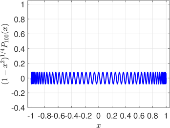
Figure 5.1. $P_{n}(x)$ and $(1-x^{2})^{\frac{1}{4}}P_{n}(x)$ with $x\in[-1,1]$ and $n=100.$

With these analysis tools at hand, we further examine $u(x)=|x|$ (as a motivative example in Trefethen [40]), for which Wang [42, 44] observed the order $O(N^{-1})$ numerically, but the order is $O(N^{-1/2})$ based on the error estimate of Legendre approximation in $L^{\infty}$-norm. From the pointwise error plots in Figure 5.2 (left), we see the largest error occurs at the singular point $x=0.$ Indeed, we have the following estimates (with the proof given in Appendix D), which are sharp as shown in Figure 5.2 (right).

Theorem 5.3.

Consider $u(x)=|x|$ for $x\in[-1,1].$ Then for $N>2,$ we have

$$\begin{split}\big{|}(u-\pi_{N}^{L}u)(0)\big{|}\leq\frac{2}{\pi(N-1)}\,;\;\quad\big{|}(u-\pi_{N}^{L}u)(\pm 1)\big{|}&\leq\frac{1}{2\sqrt{\pi}}\frac{\Gamma(N/2-1)}{\Gamma(N/2+1/2)}.\end{split}$$ (5.44)

Figure 5.2. Left: $|(u-\pi_{N}^{L}u)(x)|$ with $u(x)=|x|$ and different $N.$ Right: Tightness of the bounds in Theorem 5.3.

Finally, we apply the main results to the example $u(x)=|x|^{\mu}$ with $\mu\in(k-1,k).$ As shown in [32, Thm. 4.3], $u,u^{\prime},\ldots,u^{(k-1)}\in{\rm AC}(\bar{\Omega}),$ ${}^{C}\!D_{0+}^{\mu}u\in{\rm BV}([0,1]),$ and ${}^{C}\!D_{0-}^{\mu}u\in{\rm BV}([-1,0]).$ Thus, we infer from (5.42) that the expected convergence orders are $O(N^{-\mu+1/2})$ in $L^{\infty}$-norm and $O(N^{-\mu})$ in $L^{\infty}_{\varpi}$-norm with $\varpi=(1-x^{2})^{1/4}.$ Observe from the numerical results in Table 5.1 that the latter is optimal, but the former loses half order.

Table 5.1. Convergence order of Legendre expansion for $|x|^{\mu}$.

$N$	Errors in $L^{\infty}$-norm				Errors in $L^{\infty}_{\varpi}$-norm
	$\mu=1.7$	order	$\mu=2.6$	order	$\mu=1.7$	order	$\mu=2.6$	order
$2^{3}$	5.81e-03	–	2.35e-03	–	5.81e-03	–	2.22e-03	–
$2^{4}$	2.03e-03	1.52	4.38e-04	2.42	2.03e-03	1.52	4.38e-04	2.34
$2^{5}$	6.72e-04	1.60	8.01e-05	2.45	6.72e-04	1.60	8.01e-05	2.45
$2^{6}$	2.15e-04	1.65	1.40e-05	2.52	2.15e-04	1.65	1.40e-05	2.52
$2^{7}$	6.74e-05	1.67	2.37e-06	2.56	6.74e-05	1.67	2.37e-06	2.56
$2^{8}$	2.09e-05	1.69	3.97e-07	2.58	2.09e-05	1.69	3.97e-07	2.58

5.3. $L^{2}$-estimates

As pointed out in [38, Chap.​​ 3], the estimate of the $L^{2}$-orthogonal projection is the starting point to derive many other approximation results that provide fundamental tools for error analysis of spectral and $hp$ methods (see, e.g., [11, 16, 23, 26, 37, 38]). Most estimates therein are for functions in Sobolev or Besov spaces. Here, we consider functions with AC-BV regularity, thereby enriching the approximation theory.

We first highlight the fundamental importance of estimating $L^{2}$-orthogonal projection in (5.26). For $u\in H^{1}(\Omega),$ we define

$$(\pi_{N}^{1}u)(x)=u(-1)+\int^{x}_{-1}\pi_{N-1}^{L}u^{\prime}(t)\,{\rm d}t\in{\mathcal{P}}_{\!N},$$ (5.45)

where ${\mathcal{P}}_{\!N}$ denotes the set of polynomials of degree at most $N.$ Note that for $N\geq 2,$ we have from the orthogonality of Legendre polynomials that

$$(\pi_{N}^{1}u)(1)=u(-1)+\int^{1}_{-1}\pi_{N-1}^{L}u^{\prime}(t)\,{\rm d}t=u(-1)+\int^{1}_{-1}u^{\prime}(t)\,{\rm d}t=u(1).$$

Thus we have $(\pi_{N}^{1}u)(\pm 1)=u(\pm 1).$ Moreover, one verifies readily that

$$\int^{1}_{-1}\big{(}\pi_{N}^{1}u-u\big{)}^{\prime}(x)\,v^{\prime}(x)\,{\rm d}x=0,\;\;\;\forall v\in\mathcal{P}_{\!N}^{0}:=\{v\in{\mathcal{P}}_{\!N}:v(\pm 1)=0\}.$$

Therefore, (5.45) defines the $H^{1}_{0}$-orthogonal projection. Note that

$$\|(u-\pi_{N}^{1}u)^{\prime}\|_{L^{2}(\Omega)}^{2}=\|u^{\prime}-\pi_{N-1}^{L}u^{\prime}\|_{L^{2}({\Omega})}^{2},$$ (5.46)

so the $H^{1}$-estimate boils down to the estimate of the $L^{2}$-orthogonal projection. The high-order $H_{0}^{m}$-orthogonal projection is treated similarly in a recursive manner (see, e.g., [11]). On the other hand, the analysis of Gauss-type interpolation and quadrature errors is also based upon the Legendre expansion (see [38]).

With tools in Subsection 5.1, we can also derive the following optimal $L^{2}$-error bound under the AC-BV regularity of $u$, from which we can further establish many other approximation results indispensable for analysis of spectral and $hp$ methods for PDEs. Here, we omit such extensions.

Theorem 5.4.

Assume the conditions in Theorem 5.2 hold.

• For $\mu\in(k-1,k)$ and $-1/2<\mu<N,$

  $$\begin{split}\|u-\pi_{N}^{L}u\|_{L^{2}(\Omega)}\leq\sqrt{\frac{2}{(2\mu+1)\pi}\frac{\Gamma({N-\mu})}{\Gamma({N+\mu+1})}}\,U_{\theta}^{(\mu)}.\end{split}$$ (5.47)

• For $\mu=k,$ the estimates (5.47) hold, with the total variation $V_{\bar{\Omega}}[u^{(k)}]$ is in place of $U_{\theta}^{(\mu)}.$

Proof.

Similar to (5.34), we can use (A.3) to show that

$$\frac{\Gamma(({n-\mu})/2)}{\Gamma(({n+\mu+3})/2)}\leq\frac{\Gamma(({n-\mu-1})/2)}{\Gamma(({n+\mu})/2+1)}.$$

Then from (A.2), we derive

$$\begin{split}&\frac{(n/2+1/4)\Gamma^{2}(({n-\mu})/2)}{\Gamma^{2}(({n+\mu+3})/2)}\leq\frac{\Gamma^{2}(({n-\mu})/2)}{\Gamma(({n+\mu+3})/2)\Gamma(({n+\mu+1})/2)}\\ &\qquad\qquad\leq\frac{\Gamma(({n-\mu})/2)\Gamma(({n-\mu-1})/2)}{\Gamma(({n+\mu})/2+1)\Gamma(({n+\mu+1})/2)}=2^{2(\mu+1)}\frac{\Gamma({n-\mu-1})}{\Gamma({n+\mu+1})}\\ &\qquad\qquad=\frac{2^{2(\mu+1)}}{2\mu+1}\bigg{(}\frac{\Gamma({n-\mu-1})}{\Gamma({n+\mu})}-\frac{\Gamma({n-\mu})}{\Gamma({n+\mu+1})}\bigg{)}.\end{split}$$ (5.48)

Then, by the orthogonality of Legendre polynomials, we derive from (5.30) and (LABEL:FracL2-4) that for $\mu>-1/2$,

$$\begin{split}\big{\|}u-\pi_{N}^{L}u\big{\|}_{L^{2}(\Omega)}^{2}=&\sum_{n=N+1}^{\infty}\frac{2}{2n+1}\big{|}\hat{u}_{n}^{L}\big{|}^{2}\leq\frac{(U_{\theta}^{(\mu)})^{2}}{2^{2\mu+3}\pi}\sum_{n=N+1}^{\infty}\frac{(2n+1)\Gamma^{2}(({n-\mu})/2)}{\Gamma^{2}(({n+\mu+3})/2)}\\ \leq&\frac{2(U_{\theta}^{(\mu)})^{2}}{(2\mu+1)\pi}\frac{\Gamma({N-\mu})}{\Gamma({N+\mu+1})}.\end{split}$$ (5.49)

For $\mu=k,$ using the identity in Corollary 5.1 to derive the bound in (5.30), and then following the same lines, we can obtain the estimates in (ii). ∎

5.4. Some point-wise error estimates

In particular, the very recent work by Babuška and Hakula [10] provided some delicate point-wise estimates for the specific function (as in the seminal work [19]): $u(x)=(x-\theta)^{\beta}$ for $\theta<x\leq 1$ and $u(x)=0$ for $-1\leq x<\theta$ with $|\theta|<1$ and $\beta>0.$

Using Corollary LABEL:CorLinfL2 with $k=1$ and $V_{\bar{\Omega}}[u^{(k)}]=2$, we obtain from (LABEL:FracLinfAV2-1) and (LABEL:FracLinfBV2-1) the following estimates.

Corollary 5.2.

Consider $u(x)=|x|$ on $\bar{\Omega}.$ Then for $N\geq 1,$ we have

$$\begin{split}\big{\|}u-\pi_{N}^{L}u\big{\|}_{L^{\infty}(\Omega)}\leq\frac{4}{\sqrt{\pi}}\frac{\Gamma(N/2)}{\Gamma(N/2+1/2)},\end{split}$$ (5.50)

and

$$\begin{split}\big{\|}(1-x^{2})^{\frac{1}{4}}(u-\pi_{N}^{L}u)\big{\|}_{L^{\infty}(\Omega)}\leq\frac{4}{\pi N}.\end{split}$$ (5.51)

In fact, the estimate (5.50) is of order $O(N^{-1/2}),$ but the optimal order should be $O(N^{-1}).$ How to derive the optimal result appears open (cf. [42]). To this end, we unfold the mystery behind this.

Some important observations are in order.

• It is seen from (D) that $|P_{2m}(0)|=O(m^{-1/2}).$ However, it is overestimated in the proof of Theorem 5.2, which is bounded as $|P_{2m}(0)|\leq 1$ (see (5.33) and this type of estimates in e.g., [42, 46, 44]). This should be blamed for the loss of order at this point. Observe from Figure 5.2 (right) that the estimates are sharp.

• As shown in Figure 5.3 (left), the Legendre polynomial $P_{n}(x)$ attends its maximum/minimum at the endpoints $x=\pm 1,$ but $|P_{n}(x)|=O(n^{-1/2})$ for $x\in[-a,a]$ where $a=1-\delta$ for some small $\delta.$ In fact, we suppose to have the optimal point-wise error estimate as (5.44) for all $x\in[-a,a].$

• It is noteworthy that the (weighted) $L^{\infty}$-estimates including (5.28) in Theorem 5.2 and (LABEL:FracLinfBV2) in Corollary LABEL:CorLinfL2. As shown in Figure 5.3 (right), the extreme values of $(1-x^{2})^{\frac{1}{4}}P_{n}(x)$ behave like $O(n^{-1/2})$ as the global maximum as in (5.36). The situation is very similar to the Chebyshev polynomial. In fact, we can also see from the property (cf. [31, Thm. 2.1]): for $n>1/2$ and $\varphi\in(0,\pi),$

  $$\begin{split}(\sin\varphi)^{\frac{1}{2}}\,P_{n}(\cos\varphi)=\frac{2}{\sqrt{\pi(2n+1)}}{\cos((n+1/2)\varphi-\pi/4)}+{\mathcal{R}}_{n}(\varphi),\end{split}$$ (5.52)

  where

  $$|{\mathcal{R}}_{n}(\varphi)|\leq\frac{\sqrt{2}}{4\sqrt{\pi}(n-1/2)^{3/2}}\Big{\{}|\cot\varphi|+\frac{1}{n-1/2}\Big{\}},\quad\forall\,\varphi\in(0,\pi).$$ (5.53)

• In view of the above, we can obtain from (5.28) in Theorem 5.2 the following point-wise estimate:

  $$\begin{split}|(u-\pi_{N}^{L}u)(x)|&\leq(1-x^{2})^{-\frac{1}{4}}\|(1-x^{2})^{\frac{1}{4}}(u-\pi_{N}^{L}u\|_{L^{\infty}(\Omega)}\\ &\leq(1-x^{2})^{-\frac{1}{4}}\frac{U_{\theta}^{m,s}}{2^{\sigma-2}(\sigma-1)\pi}\frac{\Gamma(({N-\sigma})/2+1)}{\Gamma(({N+\sigma})/2)},\end{split}$$ (5.54)

  for $x\in(-1,1)$. As a result, we can derive optimal estimate for functions with interior singularities from (5.54).

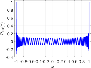
Figure 5.3. $P_{n}(x)$ and $(1-x^{2})^{\frac{1}{4}}P_{n}(x)$ with $x\in[-1,1]$ and $n=100.$

6. Legendre expansion of functions with endpoint singularities

The aforementioned AC-BV framework and main results can be extended to the study of the end-point singularities, which typically occur in underlying solutions of PDEs in various situations, for instance, irregular domains, singular coefficients and mismatch of boundary conditions among others. It is known that the Legendre expansion of a function with an endpoint singularity has a much higher convergence rate than that with an interior singularity of the same type. We illustrate this through an example which also motivates the seemingly complicated extension. To fix the idea, we focus on the left endpoint singularity but the results can be extended to the right endpoint setting straightforwardly.

6.1. An illustrative example

We consider $u(x)=(1+x)^{\mu}g(x)$ with $\mu\in(k-1,k),k\in\mathbb{N}$ and and a sufficiently smooth $g(x)$ on $\Omega.$ Then we can write

$$u(x)=(1+x)^{\mu}g(x)=\sum_{m=0}^{\infty}\frac{g^{(m)}(-1)}{m!}(1+x)^{\mu+m}.$$ (6.1)

Then by (4.8),

$$\begin{split}({}^{C}\!D_{-1+}^{\mu}u)(x)=\big{(}I_{-1+}^{k-\mu}u^{(k)}\big{)}(x)&=\sum_{m=0}^{\infty}\frac{\{\mu+m\}_{k}}{m!}g^{(m)}(-1)\,I_{-1+}^{k-\mu}\big{\{}(1+x)^{m+\mu-k}\big{\}}\\ &=\sum_{m=0}^{\infty}\frac{\{\mu+m\}_{k}\,\Gamma(m+\mu-k+1)}{(m!)^{2}}g^{(m)}(-1)\,(1+x)^{m},\end{split}$$ (6.2)

where $\{a\}_{k}=a(a-1)\cdots(a-k+1)$ stands for the falling factorial. This implies $({}^{C}\!D_{-1+}^{\mu}u)(x)$ is sufficiently smooth. In particular, if $g=1,$ then $({}^{C}\!D_{-1+}^{\mu}u)(x)$ is equal to a constant.

We deduce from Theorem 5.1 with $\theta\to-1^{+}$ that for $u,u^{\prime},\cdots,u^{(k-1)}\in{\rm AC}(\bar{\Omega}),$ and ${}^{C}\!D_{-1+}^{\mu}u\in{\rm BV}(\bar{\Omega})$ with $\mu\in(k-1,k],$ we have

$$\begin{split}\hat{u}_{n}^{L}=\frac{2n+1}{2}\Big{\{}({{}^{C}\!D_{-1+}^{\mu}u)(-1+)}(I_{1-}^{\mu+1}P_{n})(-1)+\int_{-1}^{1}(I_{1-}^{\mu+1}P_{n})(x)\,{\rm d}\big{\{}{}^{C}\!D_{-1+}^{\mu}u(x)\big{\}}\Big{\}}.\end{split}$$ (6.3)

In fact, we can show that $(I_{1-}^{\mu+1}P_{n})(-1)\sim n^{-2(\mu+1)},$ so the first term decays like $O(n^{-2\mu-1})$ (which gives the optimal convergence order for (6.1) (see Table 6.2), and doubles $O(n^{-\mu-1/2})$ for the interior singularity, e.g., of $|x|^{\mu}g(x)$).

Lemma 6.1.

For $n\geq\mu+1>0,$ we have

$$\begin{split}(I_{1-}^{\mu+1}P_{n})(-1)&=\frac{(-1)^{n}2^{\mu+1}\Gamma(\mu+1)\sin((\mu+1)\pi)}{\pi}\frac{\Gamma(n-\mu)}{\Gamma(n+\mu+2)}.\end{split}$$ (6.4)

Proof.

By (5.3), we have

$$\begin{split}&(I_{1-}^{\mu+1}P_{n})(-1)=\frac{2^{\mu+1}}{\Gamma(\mu+2)}\frac{P_{n}^{(\mu+1,-\mu-1)}(-1)}{P_{n}^{(\mu+1,-\mu-1)}(1)}=\frac{(-1)^{n}2^{\mu+1}}{\Gamma(\mu+2)}\frac{P_{n}^{(-\mu-1,\mu+1)}(1)}{P_{n}^{(\mu+1,-\mu-1)}(1)},\end{split}$$ (6.5)

where we used the parity $P_{n}^{(\alpha,\beta)}(-x)=(-1)^{n}P_{n}^{(\beta,\alpha)}(x)$ valid for all real parameters $\alpha,\beta$ (cf.​ Szegö [39, p.​ 64]). Then we derive (6.4) from (5.11) and (A.1) immediately. ∎

We find from Lemma 5.1 that the second term in (6.3) decays at a rate $O(n^{-\mu-1/2}),$ if one naively works this out with this formula. However, in view of (6.2), we can continue to carry out integration by parts upon (6.3) as many as times we want, until the first boundary term in (6.3) dominates the error. This produces the optimal order $O(n^{-2\mu-1})$ (see Table 6.2 for numerical illustrations).

Table 6.1. Decay rate of $|\hat{u}_{n}^{L}|$ with $u=(x+1)^{\mu}\sin x$.

$n$	$\mu=0.1$	order	$\mu=1.2$	order	$\mu=2.6$	order
$2^{3}$	1.26e-02	–	6.86e-04	–	1.42e-04	–
$2^{4}$	5.59e-03	1.17	6.59e-05	3.38	1.35e-06	6.72
$2^{5}$	2.47e-03	1.18	6.41e-06	3.36	1.86e-08	6.18
$2^{6}$	1.08e-03	1.19	6.20e-07	3.37	2.60e-10	6.16
$2^{7}$	4.73e-04	1.19	5.94e-08	3.38	3.49e-12	6.22

Indeed, we obtain from [32, (2.29)] that the GGF satisfies

$$\lim_{x\to-1^{+}}\big{\{}(1-x^{2})^{\sigma}\,{}^{r\!}G_{n-\sigma}^{(\sigma+1/2)}(x)\big{\}}=(-1)^{n}2^{2\sigma}\frac{\sin(\sigma\pi)}{\pi}\frac{\Gamma(\sigma)\Gamma(\sigma+1)\Gamma(n-\sigma+1)}{\Gamma(n+\sigma+1)},$$ (6.6)

where $\sigma=m+s=\alpha+1.$ Moreover, by (6.1) with $m=0,$ we have

$$\lim_{x\to-1^{+}}I_{-1+}^{1-s}\big{\{}u^{(m)}(x)\big{\}}=\Gamma(\alpha-m+1)g(-1).$$ (6.7)

Recall that (cf. [34, (5.11.13)]): for $a<b$,

$$\frac{\Gamma(z+a)}{\Gamma(z+b)}=z^{a-b}+\frac{1}{2}(a-b)(a+b-1)z^{a-b-1}+O(z^{a-b-2}),\quad z\gg 1.$$ (6.8)

Thus, the second boundary term in (6.3) for the function (LABEL:gxcase) decays like $O(n^{-2\sigma})=O(N^{-(1+2\alpha)}).$ We refer to Table 6.2 for the numerical illustration.

Table 6.2. Decay rate of $|\hat{u}_{n}^{L}|$ with $u=(x+1)^{\alpha}\sin x$.

$n$	$\alpha=0.1$	order	$\alpha=1.2$	order	$\alpha=2.6$	order
$2^{3}$	1.26e-02	–	6.86e-04	–	1.42e-04	–
$2^{4}$	5.59e-03	1.17	6.59e-05	3.38	1.35e-06	6.72
$2^{5}$	2.47e-03	1.18	6.41e-06	3.36	1.86e-08	6.18
$2^{6}$	1.08e-03	1.19	6.20e-07	3.37	2.60e-10	6.16
$2^{7}$	4.73e-04	1.19	5.94e-08	3.38	3.49e-12	6.22

Theorem 6.1 (Fractional Taylor formula).

Let $\mu\in(k-1,k]$ with $k\in\mathbb{N},$ and let $f(x)$ be a real function that is $(k-1)$times differentiable at the point $x=\theta$.

• If $f^{(k-1)}\in{\rm AC}([\theta,x]),$ let $v={}^{C}\!D_{\theta+}^{\mu}f,$ and $v,v^{\prime},\cdots,v^{(m-1)}\in{\rm AC}([\theta,x]),$ $v^{(m)}\in{\rm BV}([\theta,x])$ then we have the left-sided fractional Taylor formula

  $$\begin{split}f(x)=&\sum_{j=0}^{k-1}\frac{f^{(j)}(\theta)}{j!}(x-\theta)^{j}+(x-\theta)^{\mu}\sum_{i=0}^{m}\frac{v^{(i)}(\theta+)}{\Gamma(\mu+i+1)}{(x-\theta)^{i}}\\ &+\frac{1}{\Gamma(\mu+m+1)}\int_{\theta}^{x}(x-t)^{\mu+m}\,{\rm d}\,\{v^{(m)}(t)\}.\end{split}$$ (6.9)

• If $f^{(k-1)}\in{\rm AC}([x,\theta]),$ let $v={}^{C}\!D_{\theta-}^{\mu}f,$ and $v,v^{\prime},\cdots,v^{(m-1)}\in{\rm AC}([x,\theta]),$ $v^{(m)}\in{\rm BV}([x,\theta])$ then we have the right-sided fractional Taylor formula

  $$\begin{split}f(x)=&\sum_{j=0}^{k-1}\frac{f^{(j)}(\theta)}{j!}(x-\theta)^{j}+(\theta-x)^{\mu}\sum_{i=0}^{m}\frac{v^{(i)}(\theta-)}{\Gamma(\mu+i+1)}{(x-\theta)^{i}}\\ &-\frac{(-1)^{m}}{\Gamma(\mu+m+1)}\int^{\theta}_{x}(t-x)^{\mu+m}\,{\rm d}\,\{v^{(m)}(t)\}.\end{split}$$ (6.10)

Proof.

Using integration by parts for (4.11) and (4.12), we obtain (6.9) and (6.10), respectively. ∎

6.2. Approximation results for functions with endpoint singularities

With the above understanding, we are now ready to present the identity on the Legendre expansion coefficient from (6.3) and integration by parts. Given that the function has more regularity in this case, we make the following assumption.

Definition 6.1 (Regularity Assumption).

For $\mu\in(k-1,k]$ with $k\in\mathbb{N},$ assume $u,\cdots,u^{(k-1)}\in{\rm AC}(\bar{\Omega})$ and $v_{\mu}(x):={}^{C}\!D_{-1+}^{\mu}u\in{\rm BV}(\bar{\Omega}).$ We further assume that $v_{\mu},\cdots,v^{(m-1)}_{\mu}\in{\rm AC}(\bar{\Omega})$ and $v^{(m)}_{\mu}\in{\rm BV}(\bar{\Omega}).$ Accordingly, we denote

$$\begin{split}U^{(\mu,m)}_{-}:=V_{\bar{\Omega}}[v^{(m)}_{\mu}]+\,|\sin(\mu\pi)|\sum_{l=0}^{m}\big{|}v^{(l)}_{\mu}(-1+)\big{|}.\end{split}$$ (6.11)

For simplicity, we say $u$ is of AC-BV${}_{\!\!\mu,m}$-regularity. ∎

Note that for the example (6.1), $v_{\mu}$ is sufficiently smooth so we have $m=\infty.$ Under this assumption, we can update the formula (6.3) as follows.

Theorem 6.2.

Assume that $u$ is of AC-BV${}_{\!\!\mu,m}$-regularity. Then for $n\geq\mu+m+1,$ we have

$$\begin{split}\hat{u}_{n}^{L}&=\frac{2n+1}{2}\bigg{\{}\sum_{l=1}^{m}(I_{1-}^{\mu+l+1}P_{n})(-1)v^{(l)}_{\mu}(-1+)+\int_{-1}^{1}(I_{1-}^{\mu+m+1}P_{n})(x)\,{\rm d}\{v^{(m)}_{\mu}(x)\}\bigg{\}},\end{split}$$ (6.12)

where $(I_{1-}^{\mu+l+1}P_{n})(-1)$ has the explicit value given by (6.4).

Proof.

Since $v_{\mu},\cdots,v^{(m-1)}_{\mu}\in{\rm AC}(\bar{\Omega}),$ we can conduct integration by parts upon (6.3):

$$\begin{split}\frac{2\,\hat{u}_{n}^{L}}{2n+1}&=(I_{1-}^{\mu+1}P_{n})(-1)\,v_{\mu}(-1)+\int_{-1}^{1}(I_{1-}^{\mu+1}P_{n})(x)\,v_{\mu}^{\prime}(x)\,{\rm d}x\\ &=\cdots=\sum_{l=1}^{m-1}(I_{1-}^{\mu+l+1}P_{n})(-1)v^{(l)}_{\mu}(-1)+\int_{-1}^{1}(I_{1-}^{\mu+m}P_{n})(x)v^{(m)}_{\mu}(x)\,{\rm d}x\\ &=\sum_{l=1}^{m}(I_{1-}^{\mu+l+1}P_{n})(-1)v^{(l)}_{\mu}(-1+)+\int_{-1}^{1}(I_{1-}^{\mu+m+1}P_{n})(x)\,{\rm d}\{v^{(m)}_{\mu}(x)\},\end{split}$$

where the boundary values at $x=1$ vanish in view of (5.3), and in the last step, we used the factor $v^{(m)}_{\mu}\in{\rm BV}(\bar{\Omega})$ and (4.3). ∎

Comparing the formulas of $\hat{u}_{n}^{L}$ in Theorem 5.1 (with $\theta\to-1^{+}$, i.e., (6.3)) and Theorem 6.2, we find they largely differ from the regularity index. We can use Lemmas 5.1 and 6.1 to deal with the fractional integrals of the Legendre polynomial. Accordling, we can follow the same lines as in the proofs of Theorems 5.2 and 5.4 to derive the following estimates. To avoid the repetition, we skill the proof, though there is subtlety in some derivations.

Theorem 6.3.

Assume that $u$ is of AC-BV${}_{\!\!\mu,m}$-regularity. Then we have the following estimates.

• For $\mu>1/2$ and $N\geq\mu+m,$

  $$\begin{split}\|u-\pi_{N}^{L}u\|_{L^{\infty}(\Omega)}&\leq\bigg{\{}\frac{1}{2^{\mu+m-1}(\mu+m-1/2)\sqrt{\pi}}\frac{\Gamma(({N-\mu-m+1})/2)}{\Gamma(({N+\mu+m})/2)}\\ &\qquad+\sum_{j=0}^{m}\frac{2^{\mu+j}\Gamma(\mu+j+1)}{\pi(\mu+j-1)}\frac{\Gamma(N-\mu-j+1)}{\Gamma(N+\mu+j+1)}\bigg{\}}\,U^{(\mu,m)}_{-}.\end{split}$$ (6.13)

• For $\mu>-1/2$ and $N>\mu+m,$

  $$\begin{split}\|u-\pi_{N}^{L}u\|_{L^{2}(\Omega)}&\leq\bigg{\{}\frac{4}{(2\mu+2m+1)\pi}\frac{\Gamma({N-\mu-m})}{\Gamma({N+\mu+m+1})}\\ &\qquad+\frac{2^{6\mu+8}\Gamma^{2}(\mu+1)}{\pi^{2}(4\mu+2)}\frac{(N+1)^{2}\,\Gamma(2N-2\mu+1)}{(2N+1)^{2}\,\Gamma(2N+2\mu+3)}\bigg{\}}^{\frac{1}{2}}\,U^{(\mu,m)}_{-}.\end{split}$$ (6.14)

Proof.

(i) From Lemma 5.1 and (6.11)-(6.12), we obtain for $\mu\geq-1/2$ and $n\geq\mu+m+1,$

$$\begin{split}|\hat{u}_{n}^{L}|&\leq\bigg{\{}\frac{1}{2^{\mu+m+2}\sqrt{\pi}}\frac{(2n+1)\Gamma(({n-\mu-m})/2)}{\Gamma(({n+\mu+m+3})/2)}+\widehat{C}_{n,\mu}\sum_{j=0}^{k}\frac{\widehat{C}_{n,\mu+j}}{\widehat{C}_{n,\mu}}\bigg{\}}\,U^{(\mu,m)}_{-},\end{split}$$ (6.15)

where

$$\begin{split}\widehat{C}_{n,\mu}:&=2^{\mu}\Gamma(\mu+1)\pi^{-1}\frac{(2n+1)\Gamma(n-\mu)}{\Gamma(n+\mu+2)}.\end{split}$$ (6.16)

We now prove (6.13). By (6.15) with $|P_{n}(x)|\leq 1,$ we obtain

$$\begin{split}\big{|}(u-\pi_{N}^{L}u)(x)\big{|}&\leq\sum_{n=N+1}^{\infty}|\hat{u}_{n}^{L}|\leq\sum_{n=N+1}^{\infty}\bigg{\{}\frac{1}{2^{\mu+m+1}\sqrt{\pi}}\frac{(2n+1)\Gamma(({n-\mu-m}+1)/2)}{\Gamma(({n+\mu+m})/2+1)}\\ &\quad+\sum_{j=0}^{m}\widehat{C}_{n,\mu+j}\bigg{\}}\,U^{(\mu,m)}_{-}.\end{split}$$ (6.17)

Similar to (5.33)-(5.34), we have

$$\begin{split}\sum_{n=N+1}^{\infty}\frac{(2n+1)\Gamma(({n-\mu-m})/2)}{\Gamma(({n+\mu+m+3})/2)}\leq\frac{2}{(\mu+m-1/2)}\frac{\Gamma(({N-\mu-m+1})/2)}{\Gamma(({N+\mu+m})/2)}.\end{split}$$ (6.18)

Moreover, we can show that

$$\begin{split}\sum_{n=N+1}^{\infty}\widehat{C}_{n,\rho+1}&=\frac{2^{\rho+1}\Gamma(\rho+1)}{\pi}\sum_{n=N+1}^{\infty}\frac{(n+1/2)\Gamma(n-\rho)}{\Gamma(n+\rho+2)}\leq\frac{2^{\rho+1}\Gamma(\rho+1)}{\pi}\sum_{n=N+1}^{\infty}\frac{\Gamma(n-\rho)}{\Gamma(n+\rho+1)}\\ &=\frac{2^{\rho}\Gamma(\rho+1)}{\pi(\rho-1)}\sum_{n=N+1}^{\infty}\bigg{\{}(n+\rho)\frac{\Gamma(n-\rho)}{\Gamma(n+\rho+1)}-(n-\rho)\frac{\Gamma(n-\rho)}{\Gamma(n+\rho+1)}\bigg{\}}\\ &=\frac{2^{\rho}\Gamma(\rho+1)}{\pi(\rho-1)}\sum_{n=N+1}^{\infty}\bigg{\{}\frac{\Gamma(n-\rho)}{\Gamma(n+\rho)}-\frac{\Gamma(n-\rho+1)}{\Gamma(n+\rho+1)}\bigg{\}}=\frac{2^{\rho}\Gamma(\rho+1)}{\pi(\rho-1)}\frac{\Gamma(N-\rho+1)}{\Gamma(N+\rho+1)}.\end{split}$$ (6.19)

Thus the estimate (6.13) is a consequence of (6.17)-(6.18) and (6.19) with $\rho=\mu+j.$

(ii) We now turn to (6.14). By the orthogonality of Legendre polynomials, we find readily from (6.15) and the Cauchy-Schwarz inequality that

$$\begin{split}\big{\|}u-\pi_{N}^{L}u\big{\|}_{L^{2}(\Omega)}^{2}=&\sum_{n=N+1}^{\infty}\frac{2}{2n+1}\big{|}\hat{u}_{n}^{L}\big{|}^{2}\leq\bigg{\{}\sum_{n=N+1}^{\infty}\frac{(2n+1)\,\Gamma^{2}(({n-\mu-m})/2)}{2^{2(\mu+m+1)}\,\Gamma^{2}(({n+\mu+m}+3)/2)}\\ &\quad+\sum_{n=N+1}^{\infty}\frac{4\,\widehat{C}^{2}_{n,\mu}}{2n+1}\bigg{(}\sum_{j=0}^{m}\frac{\widehat{C}_{n,\mu+j}}{\widehat{C}_{n,\mu}}\bigg{)}^{2}\bigg{\}}\,(U^{(\mu,m)}_{-})^{2}.\end{split}$$ (6.20)

Following the derivations (LABEL:FracL2-4)-(5.49) with $\mu+m$ in place of $\mu$, we have

$$\begin{split}\sum_{n=N+1}^{\infty}\frac{(2n+1)\,\Gamma^{2}(({n-\mu-m})/2)}{\Gamma^{2}(({n+\mu+m+3})/2)}\leq\frac{2^{2\mu+2m+4}}{2\mu+2m+1}\frac{\Gamma({N-\mu-m})}{\Gamma({N+\mu+m+1})}.\end{split}$$ (6.21)

We next show that for $n\geq N+1,$

$$\begin{split}\sum_{j=0}^{m}\frac{\widehat{C}_{n,\mu+j}}{\widehat{C}_{n,\mu}}<\frac{2(N+1)}{2N+1}.\end{split}$$ (6.22)

Observe that for $1\leq i\leq j\leq m$ and $\mu+m+1\leq N+1\leq n,$

$$\begin{split}(n-\mu-i)(n+\mu+i+1)&\geq(n-\mu-j)(n+\mu+j+1)\geq(n-\mu-m)(n+\mu+m+1)\\ &\geq(n-N)(n+N+1)\geq 2(N+1).\end{split}$$

Using this inequality and (6.16), we obtain

$$\begin{split}\sum_{j=0}^{m}\frac{\widehat{C}_{n,\mu+j}}{\widehat{C}_{n,\mu}}&=\sum_{j=0}^{m}\frac{\Gamma(n-\mu-j)}{\Gamma(n-\mu)}\frac{\Gamma(n+\mu+2)}{\Gamma(n+\mu+j+2)}\\ &=1+\sum_{j=1}^{m}\bigg{(}\prod_{i=1}^{j}\frac{1}{(n-\mu-i)(n+\mu+i+1)}\bigg{)}\\ &=1+\sum_{j=1}^{m}\Big{(}\frac{1}{2(N+1)}\Big{)}^{j}<\sum_{j=0}^{\infty}\Big{(}\frac{1}{2(N+1)}\Big{)}^{j}=\frac{2(N+1)}{2N+1}.\end{split}$$ (6.23)

This yields (6.22).

Like (LABEL:FracL2-4), we can get

$$\begin{split}\frac{(n+1/2)\Gamma^{2}(n-\mu)}{\Gamma^{2}(n+\mu+2)}&\leq\frac{2^{4\mu+3}}{4\mu+2}\bigg{\{}\frac{\Gamma(2n-2\mu-1)}{\Gamma(2n+2\mu+1)}-\frac{\Gamma(2n-2\mu)}{\Gamma(2n+2\mu+2)}\bigg{\}}\\ &\leq\frac{2^{4\mu+3}}{4\mu+2}\bigg{\{}\frac{\Gamma(2n-2\mu-1)}{\Gamma(2n+2\mu+1)}-\frac{\Gamma(2n-2\mu+1)}{\Gamma(2n+2\mu+3)}\bigg{\}}.\end{split}$$

Then similar to (5.49), we have

$$\begin{split}\sum_{n=N+1}^{\infty}\frac{2}{2n+1}\widehat{C}^{2}_{n,\mu}&=\frac{2^{2\mu+2}\Gamma^{2}(\mu+1)}{\pi^{2}}\sum_{n=N+1}^{\infty}\!\!\frac{(n+1/2)\Gamma^{2}(n-\mu)}{\Gamma^{2}(n+\mu+2)}\\ &\leq\frac{2^{6\mu+5}\,\Gamma^{2}(\mu+1)}{\pi^{2}(4\mu+2)}\frac{\Gamma(2N-2\mu+1)}{\Gamma(2N+2\mu+3)}.\end{split}$$ (6.24)

Thus, we obtain (6.14) from (6.20)-(6.24). This completes the proof. ∎

In contrast to the interior singularity with a half-order loss, the $L^{\infty}$-estimate in this case is optimal. In fact, for the endpoint singularity, the largest error occurs near the boundary where $|P_{n}(x)|$ attend its maximum at $x=\pm 1$ (see Figure 5.3 (left)), so the direct summation in e.g., (5.33) will not overestimate. As an illustration, we consider $u(x)=(1+x)^{\mu}$ with $\mu\in(k-1,k),k\in\mathbb{N}$. From Theorem 6.3 and (A.5), we find $\|u-\pi_{N}^{L}u\|_{L^{\infty}(\Omega)}\leq CN^{-2\mu}$ and $\|u-\pi_{N}^{L}u\|_{L^{2}(\Omega)}\leq CN^{-2\mu-1}.$ We tabulate in Table 6.3 the errors and convergence order of Legendre approximations to $u(x)=(x+1)^{\mu}$ with various $\mu$, which indicate the optimal convergence order as predicted.

Table 6.3. Convergence of Legendre expansion of $(1+x)^{\mu}$.

$N$	Errors in $L^{\infty}$-norm				Errors in $L^{2}$-norm
	$\mu=0.1$	order	$\mu=1.2$	order	$\mu=0.1$	order	$\mu=1.2$	order
$2^{3}$	6.15e-01	–	2.27e-3	–	8.82e-3	–	2.32e-04	–
$2^{4}$	5.41e-01	0.18	4.87e-04	2.22	4.11e-03	1.10	2.64e-05	3.14
$2^{5}$	4.74e-01	0.19	9.87e-05	2.30	1.85e-03	1.15	2.75e-06	3.26
$2^{6}$	4.14e-01	0.20	1.94e-05	2.35	8.22e-04	1.17	2.74e-07	3.33
$2^{7}$	3.61e-01	0.20	3.74e-06	2.37	3.61e-04	1.19	2.67e-08	3.36
$2^{8}$	3.15e-01	0.20	7.15e-07	2.39	1.58e-04	1.19	2.56e-09	3.38

In the end of this section, we conduct the analysis similar to proof of Theorem 5.3, but for functions with endpoint singularities. We demonstrate that the estimate (6.13) in Theorem 6.3 is optimal for $u(x)=(1+x)^{\alpha},$ which is applicable to the typical singular function $u(x)=(1+x)^{\alpha}g(x)$ with smooth $g(x)$ and $g(-1)\not=0.$

Proposition 6.1.

Consider $u(x)=(x+1)^{\alpha}$ on $\bar{\Omega}$ with $\alpha>0.$ Then we have the following bounds.

• For $N>\alpha-1,$

  $$\begin{split}\big{|}(u-\pi_{N}^{L}u)(-1)\big{|}&\leq\frac{|\sin(\alpha\pi)|\,2^{\alpha}\,\Gamma(\alpha)\Gamma(\alpha+1)}{\pi}\frac{\Gamma(N-\alpha+1)}{\Gamma(N+\alpha+1)}.\end{split}$$ (6.25)

• For $N>\alpha,$

  $$\begin{split}\big{|}(u-\pi_{N}^{L}u)(1)\big{|}&\leq\frac{|\sin(\alpha\pi)|\,2^{\alpha}\,\Gamma^{2}(\alpha+1)}{\pi}\frac{\Gamma(N-\alpha)}{\Gamma(N+\alpha+1)}.\end{split}$$ (6.26)

• For $N>\alpha+3,$

  $$\begin{split}\big{|}(u-\pi_{N}^{L}u)(0)\big{|}\leq\frac{|\sin(\alpha\pi)|\,2^{\alpha+1/2}\,\Gamma^{2}(\alpha+1)}{\pi^{3/2}}\frac{\Gamma(N-\alpha-3)}{\Gamma(N+\alpha-3/2)}.\end{split}$$ (6.27)

Proof.

The proof given in Appendix LABEL:AppendixD. ∎

Figure 6.1. $|(u-\pi_{N}^{L}u)(x)|$ with $u(x)=(1+x)^{1.2}$ and different $N.$ Here, $\mathcal{B}_{1},$ $\mathcal{B}_{2},$ and $\mathcal{B}_{3}$ denote the upper bounds in (6.25)-(6.27), respectively.

Indeed, Figure 6.1 illustrates that the maximum point-wise error is attained at $x=-1,$ and the bounds in Proposition 6.1 and Theorem 6.3 agree well with the real decay of the errors. In fact, it is seen from (LABEL:unxEndSig-9) that $\hat{u}_{n}^{L}\,P_{n}(-1)$ has no sign change, so

$$|\hat{u}_{n}^{L}P_{n}(-1)|=|\hat{u}_{n}^{L}|\max\limits_{|x|\leq 1}\{|P_{n}(x)|\}=|\hat{u}_{n}^{L}|,$$

which is the key to the optimality of the estimate.

6.3. Concluding remarks

We presented a new fractional Taylor formula for singular functions whose integer-order derivatives up to $k-1$ are absolutely continuous and Caputo fractional derivative of order $\mu\in(k-1,k]$ is of bounded variation. It could be viewed as an “interpolation” between the usual Taylor formulas of two consecutive integer orders. We derived from this remarkable tool a similar fractional representation of the Legendre expansion of this type of functions, which became the cornerstone of the optimal error estimates for the Legendre orthogonal projection. The set of results under the fractional AC-BV framework greatly enriched the approximation theory for spectral and $hp$ methods. It set a good example to show how the fractional calculus could impact this classic field, and seamlessly bridge between the results valid only for integer cases. Here we merely discussed the approximation results, but this will pave the way for the analysis of and applications to singular problems, which will be a topic worthy of future deep investigation.

Appendix A Useful properties of Gamma function

Recall the Euler’s reflection formula (cf.​ [4, Ch.2]):

$$\Gamma(1-a)\Gamma(a)=\frac{\pi}{\sin(\pi a)},\quad a\not=\pm 1,\pm 2,\cdots,$$ (A.1)

and the Legendre duplication formula (cf.​ [34, (5.5.5)]):

$$\begin{split}\Gamma(2z)=\pi^{-1/2}2^{2z-1}\Gamma(z)\Gamma(z+1/2).\end{split}$$ (A.2)

From [2, (1.1) and Thm. 10], we have that for $0\leq a\leq b$, the ratio

$${\mathcal{R}}_{b}^{a}(z):=\frac{\Gamma(z+a)}{\Gamma(z+b)},\quad z\geq 0,$$ (A.3)

is decreasing with respect to $z.$ On the other hand, the ratio

$$\widehat{\mathcal{R}}_{c}(z):=\frac{1}{\sqrt{z+c}}\frac{\Gamma(z+1)}{\Gamma(z+1/2)},$$ (A.4)

is increasing (resp. decreasing) on $[-1/2,\infty)$ (resp. $(-c,\infty)$), if $c\geq 1/2$ (resp. $c\leq 1/4$), based on [14, Corollary 2].

In the error bounds, the ratio of two Gamma functions appears very often, so the following inequality is useful.

Lemma A.1.

Let $b\in(a+m,a+m+1)$ for some integer $m\geq 0,$ and set $b=a+m+\mu$ with $\mu\in(0,1).$ Then for $z+a>0$ and $z+b>1,$ we have

$$\frac{1}{(z+a)_{m}}\Big{(}z+b-\frac{3}{2}+\Big{(}\frac{5}{4}-\mu\Big{)}^{1/2}\Big{)}^{-\mu}<\frac{\Gamma(z+a)}{\Gamma(z+b)}<\frac{1}{(z+a)_{m}}\Big{(}z+b-\frac{\mu+1}{2}\Big{)}^{-\mu},$$ (A.5)

where the Pochhammer symbol: $(c)_{m}=c(c+1)\cdots(c+m-1).$

Proof.

In fact, (A.5) can be derived from the bounds in [27, (1.3)]:

$$\Big{(}x-\frac{1}{2}+\Big{(}\nu+\frac{1}{4}\Big{)}^{1/2}\Big{)}^{\nu-1}<\frac{\Gamma(x+\nu)}{\Gamma(x+1)}<\Big{(}x+\frac{\nu}{2}\Big{)}^{\nu-1},\quad x>0,\;\;\nu\in(0,1).$$ (A.6)

Indeed, using the property $\Gamma(z+1)=z\Gamma(z),$ we can write

$$\frac{\Gamma(z+a)}{\Gamma(z+b)}=\frac{1}{(z+a)_{m}}\frac{\Gamma(z+a+m)}{\Gamma(z+b)}=\frac{1}{(z+a)_{m}}\frac{\Gamma(z+b-\mu)}{\Gamma(z+b)}.$$

Then by (A.6) with $x=z+b-1$ and $\nu=1-\mu,$ we obtain (A.5) immediately. ∎

Appendix B Proof of Lemma 4.2

For $f\in L^{1}(\Omega)$ and $g\in{\rm AC}(\bar{\Omega})$, changing the order of integration by the Fubini’s Theorem, we derive from (4.16) that

$$\begin{split}&\int^{b}_{a}f(x)I_{a+}^{\rho}g^{\prime}(x)\,{\rm d}x=\frac{1}{\Gamma(\rho)}\int_{a}^{b}\bigg{\{}\int_{a}^{x}\frac{g^{\prime}(y)}{(x-y)^{1-\rho}}{\rm d}y\bigg{\}}f(x)\,{\rm d}x\\ &=\frac{1}{\Gamma(\rho)}\int_{a}^{b}\bigg{\{}\int_{y}^{b}\frac{f(x)}{(x-y)^{1-\rho}}{\rm d}x\bigg{\}}g^{\prime}(y)\,{\rm d}y=\frac{1}{\Gamma(\rho)}\int_{a}^{b}\bigg{\{}\int_{x}^{b}\frac{f(y)}{(y-x)^{1-\rho}}{\rm d}y\bigg{\}}g^{\prime}(x)\,{\rm d}x\\ &=\int^{b}_{a}g^{\prime}(x)\,I_{b-}^{\rho}f(x)\,{\rm d}x.\end{split}$$

If $I_{b-}^{\rho}f(x)\in{\rm BV}(\bar{\Omega}),$ we derive from (4.3) that

$$\begin{split}\int^{b}_{a}f(x)&\,I_{a+}^{\rho}g^{\prime}(x)\,{\rm d}x=\int^{b}_{a}g^{\prime}(x)\,I_{b-}^{\rho}f(x)\,{\rm d}x=\big{\{}g(x)\,I_{b-}^{\rho}f(x)\big{\}}\big{|}_{a^{+}}^{b^{-}}-\int^{b}_{a}g(x)\,{{\rm d}\big{\{}I_{b-}^{\rho}f(x)\big{\}}}.\end{split}$$

This yields (4.6).

We can derive (4.7) in a similar fashion.

Appendix C Proof of Proposition 4.1

Recall the first mean value theorem for the integral (cf. [47, p. 354]): Let $f,g$ be Riemman integrable on $[c,d]$, $m=\inf\limits_{x\in[c,d]}f(x),$ and $M=\sup\limits_{x\in[c,d]}f(x)$. If $g$ is nonnegative (or nonpositive) on $[c,d],$ then

$$\int_{c}^{d}f(x)g(x){\rm d}x=\kappa\int_{c}^{d}g(x){\rm d}x,\quad\kappa\in[m,M].$$ (C.1)

Recall that (cf. [36]): for $\alpha>-1$ and $\mu\in{\mathbb{R}}^{+},$

$$I_{a+}^{\mu}\,(x-a)^{\alpha}=\dfrac{\Gamma(\alpha+1)}{\Gamma(\alpha+\mu+1)}(x-a)^{\alpha+\mu}.$$ (C.2)

For any $x\in[a,a+\delta],$ we derive from (4.16), (C.1) and (C.2) that

$$\begin{split}I_{a+}^{\mu}\,u(x)&=\frac{1}{\Gamma(\mu)}\int_{a}^{x}\frac{u(y)}{(x-y)^{1-\mu}}{\rm d}y=\frac{\kappa(x)}{\Gamma(\mu)}\int_{a}^{x}\frac{(y-a)^{\alpha}}{(x-y)^{1-\mu}}{\rm d}y\\ &=\kappa(x){}_{a}I_{x}^{\mu}\,(x-a)^{\alpha}=\frac{\Gamma(\alpha+1)\kappa(x)(x-a)^{\mu+\alpha}}{\Gamma(\alpha+\mu+1)},\end{split}$$ (C.3)

where $\kappa(x)\in[m(x),M(x)]$, $m(x)=\inf\limits_{y\in[a,x]}v(y)$, $M(x)=\sup\limits_{y\in[a,x]}v(x)$. We know that

$$\lim\limits_{x\rightarrow a^{+}}m(x)=v(a),\quad\lim\limits_{x\rightarrow a^{+}}M(x)=v(a)\Rightarrow\lim\limits_{x\rightarrow a^{+}}\kappa(x)=v(a).$$ (C.4)

From (C.3) and (C.4), we obtain (4.9). This completes the proof.

Appendix D Proof of Theorem 5.3

We start with the exact formula for the Legendre expansion coefficients of $u(x)=|x|:$

$$\begin{split}\hat{u}_{2j}^{L}=\frac{(-1)^{j+1}(j+1/4)\Gamma(j-1/2)}{\sqrt{\pi}\,(j+1)!},\quad\hat{u}_{2j+1}^{L}=0,\quad j\geq 1,\end{split}$$ (D.1)

which can be derived from (5.16) with $k=1,$ i.e.,

$$\begin{split}\hat{u}_{n}^{L}&=\frac{2n+1}{2}\int^{1}_{-1}(I_{1-}^{2}P_{n})(x)\,{\rm d}\big{\{}u^{(1)}(x)\big{\}}=\frac{2n+1}{2^{2}}(I_{1-}^{2}P_{n})(0)\\ &=\frac{2n+1}{2^{5}}{}_{2}F_{1}\Big{(}\!\!-n+2,n+3;3;\frac{1}{2}\Big{)},\quad n\geq 2,\end{split}$$

and the value at $z=1/2$ (cf. [34, (15.4.28)]):

$${}_{2}F_{1}\Big{(}a,b;\frac{a+b+1}{2};\frac{1}{2}\Big{)}=\frac{\sqrt{\pi}\,\Gamma((a+b+1)/2)}{\Gamma((a+1)/2)\Gamma((b+1)/2)}.$$

Then we obtain from (D.1) that

$$\begin{split}(u-\pi_{N}^{L}u)(0)&=\sum_{j=\lceil\frac{N+1}{2}\rceil}^{\infty}\hat{u}_{2j}^{L}P_{2j}(0)=-\frac{1}{\pi}\sum_{j=\lceil\frac{N+1}{2}\rceil}^{\infty}\frac{(j+1/4)\Gamma(j-1/2)\Gamma(j+1/2)}{\Gamma(j+1)\Gamma(j+2)},\end{split}$$ (D.2)

where $\lceil\frac{N+1}{2}\rceil$ is the smallest integer $\geq\frac{N+1}{2},$ and we used the known value (cf. [39]):

$$P_{2j}(0)={}_{2}F_{1}\Big{(}\!\!-2j,2j+1;1;\frac{1}{2}\Big{)}=(-1)^{j}\frac{\Gamma(j+1/2)}{\sqrt{\pi}\,j!}.$$

From (A.3), we have

$$\frac{\Gamma(j+1/2)}{\Gamma(j+1)}\leq\frac{\Gamma(j)}{\Gamma(j+1/2)}.$$ (D.3)

Thus, using (D.3) and $\Gamma(z+1)=z\Gamma(z),$ we obtain

$$\begin{split}\frac{(j+1/4)\Gamma(j-1/2)\Gamma(j+1/2)}{\Gamma(j+1)\Gamma(j+2)}&=\frac{j+1/4}{j+1}\frac{\Gamma(j-1/2)}{\Gamma(j+1)}\frac{\Gamma(j+1/2)}{\Gamma(j+1)}\leq\frac{\Gamma(j-1/2)\Gamma(j)}{\Gamma(j+1/2)\Gamma(j+1)}\\ &=\frac{1}{(j-1/2)j}\leq\frac{1}{(j-1)j}=\frac{1}{j-1}-\frac{1}{j}.\end{split}$$

Then

$$\begin{split}&\sum_{j=\lceil\frac{N+1}{2}\rceil}^{\infty}\frac{(j+1/4)\Gamma(j-1/2)\Gamma(j+1/2)}{\Gamma(j+1)\Gamma(j+2)}\leq\sum_{j=\lceil\frac{N+1}{2}\rceil}^{\infty}\Big{(}\frac{1}{j-1}-\frac{1}{j}\Big{)}=\frac{1}{\lceil\frac{N+1}{2}\rceil-1}\leq\frac{2}{N-1}.\end{split}$$

From (D.2) and the above, we get the first result in (5.44).

We now prove the second estimate in (5.44). As $P_{n}(\pm 1)=(\pm 1)^{n},$ we derive from (D.1) that

$$\begin{split}(u-\pi_{N}^{L}u)(\pm 1)&=\sum_{j=\lceil\frac{N+1}{2}\rceil}^{\infty}\hat{u}_{2j}^{L}\,P_{2j}(\pm 1)=\sum_{j=\lceil\frac{N+1}{2}\rceil}^{\infty}\frac{(-1)^{j+1}}{\sqrt{\pi}}\frac{(j+1/4)\Gamma(j-1/2)}{\Gamma(j+2)}.\end{split}$$ (D.4)

Denoting

$$\begin{split}{\mathcal{S}}_{j}:=\frac{(-1)^{j+1}}{\sqrt{\pi}}\frac{(j+1/4)\Gamma(j-1/2)}{\Gamma(j+2)},\quad{\mathcal{T}}_{j}:=\frac{1}{2\sqrt{\pi}}\frac{\Gamma(j-3/2)}{\Gamma(j)},\end{split}$$

we have

$$\begin{split}{\mathcal{S}}_{j}+{\mathcal{S}}_{j+1}&=(-1)^{j+1}\frac{3}{2\sqrt{\pi}}\frac{(j+3/4)\Gamma(j-1/2)}{\Gamma(j+3)}\leq\frac{3}{2\sqrt{\pi}}\frac{\Gamma(j-1/2)}{\Gamma(j+2)}\\ &\leq\frac{3}{4\sqrt{\pi}}\Big{(}\frac{\Gamma(j-3/2)}{\Gamma(j+1)}+\frac{\Gamma(j-1/2)}{\Gamma(j+2)}\Big{)}=\big{(}{\mathcal{T}}_{j}-{\mathcal{T}}_{j+1}\big{)}+\big{(}{\mathcal{T}}_{j+1}-{\mathcal{T}}_{j+2}\big{)},\end{split}$$ (D.5)

where we noted

$$\begin{split}\frac{\Gamma(j-1/2)}{\Gamma(j+2)}\leq\frac{\Gamma(j-3/2)}{\Gamma(j+1)},\end{split}$$

and

$$\begin{split}\frac{3}{4\sqrt{\pi}}\frac{\Gamma(j-3/2)}{\Gamma(j+1)}=\frac{1}{2\sqrt{\pi}}\bigg{(}j\frac{\Gamma(j-3/2)}{\Gamma(j+1)}-(j-3/2)\frac{\Gamma(j-3/2)}{\Gamma(j+1)}\bigg{)}={\mathcal{T}}_{j}-{\mathcal{T}}_{j+1}.\end{split}$$

Thus from (A.3) and (D.4)-(D.5), we obtain

$$\begin{split}\big{|}(u-\pi_{N}^{L}u)(\pm 1)\big{|}&=\big{(}|{\mathcal{S}}_{\lceil\frac{N+1}{2}\rceil}+{\mathcal{S}}_{\lceil\frac{N+1}{2}\rceil+1}|\big{)}+\cdots+\big{(}|{\mathcal{S}}_{\lceil\frac{N+1}{2}\rceil+2i}+{\mathcal{S}}_{\lceil\frac{N+1}{2}\rceil+2i+1}|\big{)}+\cdots\\ &\leq\big{\{}\big{(}{\mathcal{T}}_{{\lceil\frac{N+1}{2}\rceil}}-{\mathcal{T}}_{{\lceil\frac{N+1}{2}\rceil}+1}\big{)}+\big{(}{\mathcal{T}}_{{\lceil\frac{N+1}{2}\rceil}+1}-{\mathcal{T}}_{{\lceil\frac{N+1}{2}\rceil}+2}\big{)}\big{\}}+\cdots\\ &\quad+\big{\{}\big{(}{\mathcal{T}}_{{\lceil\frac{N+1}{2}\rceil}+2i}-{\mathcal{T}}_{{\lceil\frac{N+1}{2}\rceil}+2i+1}\big{)}+\big{(}{\mathcal{T}}_{{\lceil\frac{N+1}{2}\rceil}+2i+1}-{\mathcal{T}}_{{\lceil\frac{N+1}{2}\rceil}+2i+2}\big{)}\big{\}}+\cdots\\ &=\sum_{j=\lceil\frac{N+1}{2}\rceil}^{\infty}\big{(}{\mathcal{T}}_{j}-{\mathcal{T}}_{j+1}\big{)}=\frac{1}{2\sqrt{\pi}}\frac{\Gamma(\lceil\frac{N+1}{2}\rceil-3/2)}{\Gamma(\lceil\frac{N+1}{2}\rceil)}\leq\frac{1}{2\sqrt{\pi}}\frac{\Gamma(N/2-1)}{\Gamma(N/2+1/2)}.\end{split}$$

This ends the proof.

References

- [1] R.A. Adams. Sobolev Spaces. Academic Press, New York, 1975.
- [2] H. Alzer. On some inequalities for the Gamma and Psi functions. Math. Comput., 66(217):373–389, 1997.
- [3] G.A. Anastassiou. On right fractional calculus. Chaos Solitons Fractals, 42(1):365–376, 2009.
- [4] G.E. Andrews, R. Askey, and R. Roy. Special Functions, Encyclopedia of Mathematics and its Applications, Vol. 71. Cambridge University Press, Cambridge, 1999.
- [5] V.A. Antonov and K.V. Holsevnikov. An estimate of the remainder in the expansion of the generating function for the Legendre polynomials (Generalization and improvement of Bernstein’s inequality). Vestn. Leningr. Univ. Math., 13:163–166, 1981.
- [6] J. Appell, J. Banaś, and N. Merentes. Bounded Variation and Around. Walter de Gruyter, Berlin, 2014.
- [7] I. Babuška and B.Q. Guo. Optimal estimates for lower and upper bounds of approximation errors in the -version of the finite element method in two dimensions. Numer. Math., 85(2):219–255, 2000.
- [8] I. Babuška and B.Q. Guo. Direct and inverse approximation theorems for the -version of the finite element method in the framework of weighted Besov spaces I: Approximability of functions in the weighted Besov spaces. SIAM J. Numer. Anal., 39(5):1512–1538, 2001.
- [9] I. Babuška and B.Q. Guo. Direct and inverse approximation theorems for the -version of the finite element method in the framework of weighted Besov spaces, Part II: Optimal rate of convergence of the -version finite element solutions. Math. Models Methods Appl. Sci., 12(5):689–719, 2002.
- [10] I. Babuška and H. Hakula. Pointwise error estimate of the Legendre expansion: the known and unknown features. Comput. Methods Appl. Mech. Engrg., 345:748–773, 2019.
- [11] C. Bernardi and Y. Maday. Spectral Methods. In P.G. Ciarlet and J.L. Lions, editors, Handbook of Numerical Analysis, pages 209–486. Elsevier, Amsterdam, 1997.
- [12] L. Bourdin and D. Idczak. A fractional fundamental lemma and a fractional integration by parts formula-applications to critical points of Bolza functionals and to linear boundary value problems. Adv. Differential Equations, 20(3–4):213–232, 2015.
- [13] H. Brezis. Functional Analysis, Sobolev Spaces and Partial Differential Equations. Springer, New York, 2011.
- [14] J. Bustoz and M.E.H. Ismail. On Gamma function inequalities. Math. Comput., 47(176):659–667, 1986.
- [15] G. Buttazzo, M. Giaquinta, and S. Hildebrandt. One-Dimensional Variational Problems: An Introduction. Oxford University Press, New York, 1998.
- [16] C. Canuto, M.Y. Hussaini, A. Quarteroni, and T.A. Zang. Spectral Methods: Fundamentals in Single Domains. Springer, Berlin, 2006.
- [17] M. Carter and B. van Brunt. The Lebesgue-Stieltjes Integral: A Practical Introduction. Springer, New York, 2000.
- [18] D. Funaro. Polynomial Approxiamtions of Differential Equations. Springer-Verlag, 1992.
- [19] W. Gui and I. Babuška. The and - versions of the finite element method in dimension. I. The error analysis of the -version. Numer. Math., 49(6):577–612, 1986.
- [20] W. Gui and I. Babuška. The and - versions of the finite element method in dimension. II. The error analysis of the - and - versions. Numer. Math., 49(6):613–657, 1986.
- [21] W. Gui and I. Babuška. The and - versions of the finite element method in dimension. III. The adaptive - version. Numer. Math., 49(6):659–683, 1986.
- [22] B.Q. Guo and I. Babuška. Direct and inverse approximation theorems for the -version of the finite element method in the framework of weighted Besov spaces, part III: Inverse approximation theorems. J. Approx. Theory, 173:122–157, 2013.
- [23] B.Y. Guo. Spectral Methods and Their Applications. World Scientific, Singapore, 1998.
- [24] B.Y. Guo, J. Shen, and L.-L. Wang. Optimal spectral-Galerkin methods using generalized Jacobi polynomials. J. Sci. Comput., 27:305–322, 2006.
- [25] B.Y. Guo and L.-L. Wang. Jacobi approximations in non-uniformly Jacobi-weighted Sobolev spaces. J. Approx. Theory, 128(1):1–41, 2004.
- [26] J. Hesthaven, S. Gottlieb, and D. Gottlieb. Spectral Methods for Time-Dependent Problems. Cambridge University Press, Cambridge, 2007.
- [27] D. Kershaw. Some extensions of W. Gautschi’s inequalities for the Gamma function. Math. Comp., 41(164):607–611, 1983.
- [28] F.C. Klebaner. Introduction to Stochastic Calculus with Applications, 3nd Ed. Imperial College Press, London, 2012.
- [29] K.M. Kolwankar and A.D. Gangal. Local fractional Fokker-Planck equation. Phys. Rev. Lett., 80(2):214–217, 1998.
- [30] S. Lang. Real and Functional Analysis, 3rd Ed. Springer, New York, 1993.
- [31] W.J. Liu and L.-L. Wang. Asymptotics of the generalized Gegenbauer functions of fractional degree. J. Approx. Theory, 253:105378, 2020.
- [32] W.J. Liu, L.-L. Wang, and H.Y. Li. Optimal error estimates for Chebyshev approximations of functions with limited regularity in fractional Sobolev-type spaces. Math. Comp., 88(320):2857–2895, 2019.
- [33] H. Majidian. On the decay rate of Chebyshev coefficients. Appl. Numer. Math., 113:44–53, 2017.
- [34] F.W.J. Olver, D.W. Lozier, R.F. Boisvert, and C.W. Clark. NIST Handbook of Mathematical Functions. Cambridge University Press, New York, 2010.
- [35] S. Ponnusamy. Foundations of Mathematical Analysis. Springer, New York, 2012.
- [36] S.G. Samko, A.A. Kilbas, and O.I. Marichev. Fractional Integrals and Derivatives, Theory and Applications. Gordan and Breach Science Publisher, New York, 1993.
- [37] C. Schwab. - and -FEM. Theory and Application to Solid and Fluid Mechanics. Oxford University Press, New York, 1998.
- [38] J. Shen, T. Tang, and L.-L. Wang. Spectral Methods: Algorithms, Analysis and Applications. Springer-Verlag, New York, 2011.
- [39] G. Szegö. Orthogonal Polynomials, 4th Ed. Amer. Math. Soc., Providence, RI, 1975.
- [40] L.N. Trefethen. Is Gauss quadrature better than Clenshaw-Curtis? SIAM Rev., 50(1):67–87, 2008.
- [41] L.N. Trefethen. Approximation Theory and Approximation Practice. SIAM, Philadelphia, 2013.
- [42] H.Y. Wang. A new and sharper bound for Legendre expansion of differentiable functions. Appl. Math. Lett., 85:95–102, 2018.
- [43] H.Y. Wang. On the convergence rate of Clenshaw-Curtis quadrature for integrals with algebraic endpoint singularities. J. Comput. Appl. Math., 333:87–98, 2018.
- [44] H.Y. Wang. How fast does the best polynomial approximation converge than Legendre projection? arXiv:2001.01985v2, 2020.
- [45] S.H. Xiang and F. Bornemann. On the convergence rates of Gauss and Clenshaw-Curtis quadrature for functions of limited regularity. SIAM J. Numer. Anal., 50(5):2581–2587, 2012.
- [46] S.H. Xiang and G.D. Liu. Optimal decay rates on the asymptotics of orthogonal polynomial expansions for functions of limited regularities. Numer. Math., 145:117–148, 2020.
- [47] V.A. Zorich. Mathematical Analysis I, 2nd Ed. Springer-Verlag, Berlin, 2016.