Submodular Bandit Problem Under Multiple Constraints

Abstract

The linear submodular bandit problem was proposed to simultaneously address diversified retrieval and online learning in a recommender system. If there is no uncertainty, this problem is equivalent to a submodular maximization problem under a cardinality constraint. However, in some situations, recommendation lists should satisfy additional constraints such as budget constraints, other than a cardinality constraint. Thus, motivated by diversified retrieval considering budget constraints, we introduce a submodular bandit problem under the intersection of $l$ knapsacks and a $k$-system constraint. Here $k$-system constraints form a very general class of constraints including cardinality constraints and the intersection of $k$ matroid constraints. To solve this problem, we propose a non-greedy algorithm that adaptively focuses on a standard or modified upper-confidence bound. We provide a high-probability upper bound of an approximation regret, where the approximation ratio matches that of a fast offline algorithm. Moreover, we perform experiments under various combinations of constraints using a synthetic and two real-world datasets and demonstrate that our proposed methods outperform the existing baselines.

1 INTRODUCTION

The multi-armed bandit (MAB) problem has been widely used for practical applications. Examples include interactive recommender systems, Internet advertising, portfolio selection, and clinical trials. In a typical MAB problem, the agent selects one arm in each round. However, in practice, it is more convenient to select more than one arm in each round. Such a problem is called a combinatorial bandit problem [Chen et al., 2013]. For example, in [Yue and Guestrin, 2011, Radlinski et al., 2008], they considered the problem where in each round, the agent proposes multiple news articles or web documents to a user.

When recommending multiple items to a user, agents should select well-diversified items to maximize coverage of the information the user finds interesting [Yue and Guestrin, 2011] or to reduce item similarity in the list [Ziegler et al., 2005]. Recommending redundant items leads to diminishing returns in terms of utility [Yu et al., 2016]. It is well-known that properties such as diversity or diminishing returns are well captured by submodular set functions [Krause and Golovin, 2014]. To simultaneously address diversified retrieval and online learning in a recommender system, Yue and Guestrin [2011] proposed a combinatorial bandit problem (or more specifically a semi-bandit problem), called the linear submodular bandit problem, where in each round a sequence rewards are generated by an unknown submodular function.

For a real-world application, recommendation lists should satisfy several constraints. We explain this by using a news article recommendation example. For a comfortable user experience while selecting news articles from a recommendation list, the length of the list should not be excessively long, which implies that the list should satisfy a cardinality constraint. Furthermore, a user may not wish to spend more than a certain amount of time by reading news articles. This can be modeled as a knapsack constraint. With only a knapsack constraint, a system can recommend a long list of short (or low cost) news articles. However, due to the space constraint of the web site, such a list cannot be displayed. Therefore, it is necessary to consider a submodular bandit problem under the intersection of the knapsack and cardinality constraints.

Yue and Guestrin [2011] introduced a submodular bandit problem under a cardinality constraint and proposed an algorithm called LSBGreedy. Later, Yu et al. [2016] considered a submodular bandit problem under a knapsack constraint and proposed two greedy algorithms called MCSGreedy and CGreedy. However, such existing algorithms fail to properly optimize the objective function under complex constraints. In fact, we theoretically and empirically show that such simple greedy algorithms can perform poorly.

Under a simple constraint such as a cardinality or a knapsack constraint, there is a simple rule to select elements. This rule is called the upper confidence bound (UCB) rule or the modified UCB rule if the constraint is a cardinality or a knapsack constraint, respectively [Yu et al., 2016]. For example, with the UCB rule, the algorithm selects the element with the largest UCB sequentially in each round. Considering that our problem is a generalization of both the problems, we should generalize both the rules.

In this study, we solve the problem under a more generalized constraint, i.e., the intersection of $l$ knapsacks and $k$-system constraints. Here, the $k$-system constraints form a very general class of constraints, including cardinality constraints and the intersection of $k$ matroid constraints. For example, when recommending news articles, we can restrict the number of news articles from each topic with a $k$-system constraint. To solve the problem, we propose a non-greedy algorithm that adaptively focuses on the UCB and modified UCB rules. Since the submodular maximization problem is NP-hard, we theoretically evaluate our method by an $\alpha$-approximation regret, where $\alpha\in(0,1)$ is an approximation ratio. In this study, we provide an upper bound of the $\alpha$-approximation regret in the case when $\alpha=\frac{1}{(1+\varepsilon)(k+2l+1)}$, where $\varepsilon$ is a parameter of the algorithm. We note that the approximation ratio matches that of an offline algorithm [Badanidiyuru and Vondrák, 2014]. To the best of our knowledge, no known offline algorithm achieves a better approximation ratio than $\alpha$ above and better computational complexity than the offline algorithm, simultaneously . More precisely, our contributions are stated as follows:

OUR CONTRIBUTIONS

1. We propose a submodular bandit problem with semi-bandit feedback under the intersection of $l$ knapsacks and $k$-system constraints (Section 4). This is the first attempt to solve the submodular bandit problem under such complex constraints. The problem is new even when the $k$-system constraint is a cardinality constraint.

2. We propose a novel algorithm called AFSM-UCB that Adaptively Focuses on a Standard or Modified Upper Confidence Bound (Section 5).

3. We provide a high-probability upper bound of an approximation regret for AFSM-UCB (Section 6). We prove that the $\alpha$-approximation regret $\mathrm{Reg}_{\alpha}\left(T\right)$ is given by $O(\sqrt{mT}\ln(mT/\delta))$ with probability in least $1-\delta$ and the computational complexity in each round is given as $O(m|\mathcal{N}|\ln|\mathcal{N}|/\ln(1+\varepsilon))$, where $\alpha=\frac{1}{(1+\varepsilon)(k+2l+1)}$, $\varepsilon$ is a parameter of the algorithm, $T$ is the time horizon, $m$ is the cardinality of a maximal feasible solution, and $\mathcal{N}$ is the ground set (e.g., the set of all news articles in the news recommendation example). We note that no known offline fast algorithm achieves a better approximation ratio than above.

4. We empirically prove the effectiveness of our proposed method by comprehensively evaluating it on a synthetic and two real-world datasets. We show that our proposed method outperforms the existing greedy baselines such as LSBGreedy and CGreedy.

2 RELATED WORK

2.1 SUBMODULAR MAXIMIZATION

Although submodular maximization has been studied over four decades, we introduce only recent results relevant to our work. Badanidiyuru and Vondrák [2014] provided a maximization algorithm for a non-negative, monotone submodular function with $l$ knapsack constraints and a $k$-system constraint that achieves $\frac{1}{(1+\varepsilon)(k+2l+1)}$-approximation solution. Based on this work and Gupta et al. [2010], Mirzasoleiman et al. [2016] proposed a maximization algorithm called FANTOM under the same constraint in the case when the objective function is not necessarily monotone. Our proposed method is inspired by these two offline algorithms. However, because of uncertainty due to semi-bandit feedback, we need a nontrivial modification. A key feature of our method and aforementioned two offline algorithms is that they filter out “bad” elements via a threshold. Such a threshold method is also used for other problem settings such as streaming submodular maximization under a cardinality constraint [Badanidiyuru et al., 2014]. Some algorithms [Sarpatwar et al., 2019, Chekuri et al., 2010, 2014] achieves better approximation ratios than that of [Badanidiyuru and Vondrák, 2014] under narrower classes of constraints (e.g., a matroid + $l$ knapsacks). However, these algorithms are not “fast” because their computational complexity is $O(\mathrm{poly}(|\mathcal{N}|))$ with a polynomial of high degree, while that of [Badanidiyuru and Vondrák, 2014] is $O(\frac{|\mathcal{N}|}{\varepsilon^{2}}\ln^{2}\frac{|\mathcal{N}|}{\varepsilon})$. For example, the computational complexity of the algorithm provided in [Sarpatwar et al., 2019] is $\widetilde{O}(|\mathcal{N}|^{6})$ when $k=1$. We refer to [Sarpatwar et al., 2019, Mirzasoleiman et al., 2016] for further comparison with respect to an approximation ratio and computational complexity.

2.2 SUBMODULAR BANDIT PROBLEMS

Yue and Guestrin [2011] introduced the linear submodular bandit problem to solve a diversification problem in a retrieval system and proposed a greedy algorithm called LSBGreedy. Later, Yu et al. [2016] considered a variant of the problem, that is, the linear submodular bandit problem with a knapsack constraint and proposed two greedy algorithms called MCSGreedy and CGreedy. Chen et al. [2017] generalized the linear submodular bandit problem to an infinite dimensional case, i.e., in the case where the marginal gain of the score function belongs to a reproducing kernel Hilbert space (RKHS) and has a bounded norm in the space. Then, they proposed a greedy algorithm called SM-UCB. Recently, Hiranandani et al. [2019] studied a model combining linear submodular bandits with a cascading model [Craswell et al., 2008]. Strictly speaking, their objective function is not a submodular function. Table 1 shows a comparison with other submodular bandit problems with respect to constraints.

Table 1: Comparison of other submodular bandit algorithms with respect to constraints.

Methods	Cardinality	Knapsack	$k$-system
LSBGreedy	✓
CGreedy		✓
SM-UCB	✓
Our method	✓	✓	✓

3 DEFINITION

In this section, we provide definitions of terminology used in this paper. Throughout this paper, we fix a finite set $\mathcal{N}$ called a ground set that represents the set of the entire news articles in the news article recommendation example.

3.1 SUBMODULAR FUNCTION

In this subsection, we define submodular functions. We refer to [Krause and Golovin, 2014] for an introduction to this subject.

We denote by $2^{\mathcal{N}}$ the set of subsets of $\mathcal{N}$. For $e\in\mathcal{N}$ and $S\subseteq\mathcal{N}$, we write $S+e=S\cup\left\{e\right\}$. Let $f:2^{\mathcal{N}}\rightarrow\mathbb{R}$ be a set function. We call $f$ a submodular function if $f$ satisfies $\Delta f(e|A)\geq\Delta f(e|B)$ for any $A,B\in 2^{\mathcal{N}}$ with $A\subseteq B$ and for any $e\in\mathcal{N}\setminus B$. Here, $\Delta f(e|A)$ is the marginal gain when $e$ is added to $A$ and defined as $f(A+e)-f(A)$. We note that a linear combination of submodular functions with non-negative coefficients is also submodular. A submodular function $f$ on $2^{\mathcal{N}}$ is called monotone if $f(B)\geq f(A)$ for any $A,B\in 2^{\mathcal{N}}$ with $A\subseteq B$. A set function $f$ on $2^{\mathcal{N}}$ is called non-negative if $f(S)\geq 0$ for any $S\subseteq\mathcal{N}$. Although non-monotone submodular functions have important applications [Mirzasoleiman et al., 2016], we consider only non-negative, monotone submodular functions in this study as in the preceding work [Yue and Guestrin, 2011, Yu et al., 2016, Chen et al., 2017].

Many useful and interesting functions satisfy submodularity. Examples include coverage functions, probabilistic coverage functions [El-Arini et al., 2009], entropy and mutual information [Krause and Guestrin, 2005] under an assumption and ROUGE [Lin and Bilmes, 2011].

3.2 MATROID, $k$-SYSTEM, AND KNAPSACK CONSTRAINTS

For succinctness, we omit formal definitions of the matroid and $k$-system. Instead, we introduce examples of matroids and remark that the intersection of $k$ matroids is a $k$-system. For definitions of these notions, we refer to [Calinescu et al., 2011].

First, we provide an important example of a matroid. Let $\mathcal{N}_{i}\subseteq\mathcal{N}$ ($i=1,\dots,n$) be a partition of $\mathcal{N}$, that is $\mathcal{N}$ is the disjoint union of these subsets. For $1\leq i\leq n$, we fix a non-negative integer $d_{i}$ and let $\mathcal{P}=\left\{S\in 2^{\mathcal{N}}\mid|S\cap\mathcal{N}_{i}|\leq d_{i},\ \forall i\right\}$. Then, the pair $(\mathcal{N},\mathcal{P})$ is an example of a matroid and called a partition matroid. Let $d$ be a non-negative integer and put $\mathcal{U}=\left\{S\in 2^{\mathcal{N}}\mid|S|\leq d\right\}$. Then $(\mathcal{N},\mathcal{U})$ is a special case of partition matroids and called a uniform matroid. Let $(\mathcal{N},\mathcal{M}_{i})$ for $1\leq i\leq k$ be $k$ matroids, where $\mathcal{M}_{i}\subseteq 2^{\mathcal{N}}$. The intersection of matroids $(\mathcal{N},\cap_{i=1}^{k}\mathcal{M}_{i})$ is not necessarily a matroid but a $k$-system (or more specifically it is a $k$-extendible system) [Calinescu et al., 2011, Mestre, 2006, 2015]. In particular, any matroid is a $1$-system. For a $k$-system $(\mathcal{N},\mathcal{I})$ with $\mathcal{I}\subseteq 2^{\mathcal{N}}$ and a subset $S\subseteq\mathcal{N}$, we say that $S$ satisfies the $k$-system constraint if and only if $S\in\mathcal{I}$. Trivially, a uniform matroid constraint is equivalent to a cardinality constraint.

Next, we provide a definition of knapsack constraint. Let $c:\mathcal{N}\rightarrow\mathbb{R}_{>0}$ be a function. For $e\in\mathcal{N}$, we suppose $c(e)$ represents the cost of $e$. Let $b\in\mathbb{R}_{>0}$ be a budget and $S\subseteq\mathcal{N}$ a subset. We say that $S$ satisfies the knapsack constraint with the budget $b$ if $c(S):=\sum_{e\in S}c(e)\leq b$. Without loss of generality, it is sufficient to consider the unit budget case, i.e., $b=1$.

4 PROBLEM FORMULATION

Throughout this paper, we consider the following intersection of $l$ knapsacks and $k$-system constraints:

$$c_{j}(S)\leq 1\ (1\leq\forall j\leq l)\quad\text{ and }S\in\mathcal{I}$$ (1)

Here for $1\leq j\leq l$, $c_{j}:\mathcal{N}\rightarrow\mathbb{R}_{>0}$ is a cost and $(\mathcal{N},\mathcal{I})$ is a $k$-system.

In this study, we consider the following sequential decision-making process for times steps $t=1,\dots,T$.

(i) The algorithm selects a list $S_{t}=\left\{e^{(1)}_{t},\allowbreak\dots,\allowbreak e^{(m_{t})}_{t}\right\}\subseteq\mathcal{N}$ satisfying the constraints (1).

(ii) The algorithm receives noisy rewards $y_{t}^{(1)},\dots,y_{t}^{(m_{t})}$ as follows:

$$y_{t}^{(i)}=\Delta f\left(e_{t}^{(i)}\mid S_{t}^{(1:i-1)}\right)+\varepsilon_{t}^{(i)},\text{ for }i=1,\dots,m_{t},$$

Here $f$ is a submodular function unknown to the algorithm, $S_{t}^{(1:i-1)}=\left\{e_{t}^{(1)},\allowbreak\dots,\allowbreak e_{t}^{(i-1)}\right\}$ and $\varepsilon_{t}^{(i)}$ is a noise. We regard $S_{t}^{(1:i-1)}$, $e_{t}^{(i-1)}$ and $\varepsilon_{t}^{(i)}$ as random variables. The objective of the algorithm is to maximize the sum of rewards $\sum_{t=1}^{T}f(S_{t})$.

Following [Yue and Guestrin, 2011], we explain this problem by using the news article recommendation example. In each round, the user scans the list of the recommended items $S_{t}=\left\{e_{t}^{(1)},\dots,e_{t}^{(m_{t})}\right\}$ one-by-one in top-down fashion, where $m_{t}$ is the cardinality of $S_{t}$ at round $t$. We assume that the marginal gain $\Delta f(e_{t}^{(i)}\mid S_{t}^{(1:i-1)})$ represents the new information covered by $e_{t}^{(i)}$ and not covered by $S_{t}^{(1:i-1)}$. The noisy rewards $y_{t}^{(1)},\dots,y_{t}^{(m_{t})}$ are binary random variables and the user likes $e_{t}^{(i)}$ with probability $\Delta f(e_{t}^{(i)}\mid S_{t}^{(1:i-1)})$.

4.1 ASSUMPTIONS ON THE SCORE FUNCTION $f$

Following [Yue and Guestrin, 2011], we assume that there exist $d$ known submodular functions $f_{1},\dots,f_{d}$ on $2^{\mathcal{N}}$ that are linearly independent and the objective submodular function $f$ can be written as a linear combination $f=\sum_{i=1}^{d}w_{i}f_{i}$, where the coefficients $w_{1},\dots,w_{d}$ are non-negative and unknown to the algorithm. We fix a parameter $B>0$ and assume that $\sqrt{\sum_{i=1}^{d}w_{i}^{2}}\leq B$. We also assume that for some $A>0$, the $L^{2}$-norm of vector $[\Delta f_{i}(e\mid S)]_{i=1}^{d}$ is bounded above by $\sqrt{A}$ for any $e\in\mathcal{N}$ and $S\in 2^{\mathcal{N}}$.

We note that this can be generalized to an infinite dimensional case as in [Chen et al., 2017]. We discuss this setting more in detail in the supplemental material and provide a theoretical result in this setting.

4.2 ASSUMPTIONS ON NOISE STOCHASTIC PROCESS

We assume that there exists $m\in\mathbb{Z}_{>0}$ such that $m_{t}\leq m$ for all $t$ and consider the lexicographic order on the set $\left\{(t,i)\mid t=1,\allowbreak\dots,\allowbreak\ 1\leq i\leq m\right\}$, i.e., $(t,i)\leq(t^{\prime},i^{\prime})$ if and only if either $t<t^{\prime}$ or $t=t^{\prime}$ and $i\leq i^{\prime}$. Then, we can identify the set with the set of natural numbers (as ordered sets) and can regard $\{\varepsilon_{t}^{(i)}\}_{t,i}$ as a sequence. We assume that the stochastic process $\left\{\varepsilon_{t}^{(i)}\right\}_{t,i}$ is conditionally $R$-sub-Gaussian for a fixed constant $R\geq 0$, i.e., $\mathbf{E}\left[\exp\left(\xi\varepsilon_{t}^{(i)}\right)\mid\mathcal{F}_{t,i}\right]\leq\exp\left(\frac{\xi^{2}R^{2}}{2}\right),$ for any $(t,i)$ and any $\xi\in\mathbb{R}$. Here, $\mathcal{F}_{t,i}$ is the $\sigma$-algebra generated by $\left\{S_{u}^{(1:j)}\mid(u,j)<(t,i)\right\}$ and $\left\{\varepsilon_{u}^{(j)}\mid(u,j)<(t,i)\right\}$. This is a standard assumption on the noise sequence [Chowdhury and Gopalan, 2017, Abbasi-Yadkori et al., 2011]. For example, if $\{\varepsilon_{t}^{(i)}\}$ is a martingale difference sequence and $|\varepsilon_{t}^{(i)}|\leq R$ or $\{\varepsilon_{t}^{(i)}\}$ is conditionally Gaussian with zero mean and variance $R^{2}$, then the condition is satisfied [Lattimore and Szepesvári, 2019].

4.3 APPROXIMATION REGRET

As usual in the combinatorial bandit problem, we evaluate bandit algorithms by a regret called $\alpha$-approximation regret (or $\alpha$-regret in short), where $\alpha\in(0,1)$. The approximation regret is necessary for meaningful evaluation. Even if the submodular function $f$ is completely known, it has been proved that no algorithm can achieve the optimal solution by evaluating $f$ in polynomial time [Nemhauser and Wolsey, 1978].

We denote by $OPT$ the optimal solution, i.e., $OPT=\operatorname{argmax}_{S}f(S),$ where $S$ runs over $2^{\mathcal{N}}$ satisfying the constraint (1). We define the $\alpha$-regret as follows:

$$\mathrm{Reg}_{\alpha}\left(T\right)=\sum_{t=1}^{T}\left\{\alpha f(OPT)-f(S_{t})\right\}.$$

This definition is slightly different from that given in [Yue and Guestrin, 2011] because our definition does not include noise as in [Chowdhury and Gopalan, 2017]. In either case, one can prove a similar upper bound. For the proof in the cardinality constraint case, we refer to Lemma 4 in the supplemental material of [Yue and Guestrin, 2011].

In this study, we take the same approximation ratio $\alpha=\frac{1}{(1+\varepsilon)(k+2l+1)}$ as that of a fast algorithm in the offline setting [Badanidiyuru and Vondrák, 2014, Theorem 6.1]. As mentioned in Section 2, there exist offline algorithms that achieve better approximation ratios than above, but they have high computational complexity. Later, we remark that our proposed method is also “fast”.

5 ALGORITHM

In this section, following [Yue and Guestrin, 2011, Yu et al., 2016], we first define a UCB score of the marginal gain $\Delta f(e\mid S)$ and introduce a modified UCB score. With a UCB score, one can balance the exploitation and exploration tradeoff with bandit feedback. Then, we propose a non-greedy algorithm (Algorithm 2) that adaptively focuses on the UCB score and modified UCB score.

5.1 UCB SCORES

For $e\in\mathcal{N}$ and $S\in 2^{\mathcal{N}}$, we define a column vector $x(e\mid S)$ by $\left(\Delta f_{i}(e\mid S)\right)_{i=1}^{d}\in\mathbb{R}^{d}$ and put $x_{t}^{(i)}=x\left(e^{(i)}_{t}\mid S_{t}^{(1:i-1)}\right)$. Here, we use the same notation as in Section 4. We define $b_{t},w_{t}\in\mathbb{R}^{d}$ and $M_{t}\in\mathbb{R}^{d\times d}$ as follows:

$$b_{t} :=\sum_{s=1}^{t}\sum_{i=1}^{m_{s}}y_{s}^{(i)}x_{s}^{(i)},$$

$$M_{t} :=\lambda I+\sum_{s=1}^{t}\sum_{i=1}^{m_{s}}x_{s}^{(i)}\otimes x_{s}^{(i)}, w_{t}:=M_{t}^{-1}b_{t},$$

Here, $\lambda>0$ is a parameter of the model and for a column vector $x\in\mathbb{R}^{d}$, we denote by $x\otimes x\in\mathbb{R}^{d\times d}$ the Kronecker product of $x$ and $x$.

For $e\in\mathcal{N}$ and $S\in 2^{\mathcal{N}}$, we define $\mu(e\mid S):=w_{t}\cdot x(e\mid S)$ and $\sigma(e\mid S):=\sqrt{x(e|S)^{\mathrm{T}}\hskip 2.0ptM_{t}^{-1}\hskip 2.0ptx(e|S)}.$ Then, we define a UCB score of the marginal gain by

$$\mathrm{ucb}_{t}(e\mid S)=\mu_{t-1}(e\mid S)+\beta_{t-1}\sigma_{t-1}(e\mid S),$$

and a modified UCB score by $\mathrm{ucb}_{t}(e\mid S)/c(e)$. Here,

$$\beta_{t}:=B+R\sqrt{\ln\det\left(\lambda^{-1}M_{t}\right)+2+2\ln(1/\delta)},$$

and $c(e):=\sum_{j=1}^{l}c_{j}(e)$. It is well-known that $\mathrm{ucb}_{t}(e\mid\phi,S)$ is an upper confidence bound for $\Delta f_{\phi}(e\mid S)$. More precisely, we have the following result.

Proposition 1.

We assume there exists $m\in\mathbb{Z}_{\geq 1}$ such that $m_{t}\leq m$ for all $1\ \leq t\leq T$. We also assume that $\lambda\geq L$. Then, with probability at least $1-\delta$, the following inequality holds:

$$\left|\mu_{t-1}(e\mid S)-\Delta f(e\mid S)\right|\leq\beta_{t-1}\sigma_{t-1}(e\mid S),$$

for any $t,S,$ and $e$.

Proposition 1 follows from the proof of [Chowdhury and Gopalan, 2017, Theorem 2]. We note that this theorem is a more generalized result than the statement above (they do not assume that the objective function is linear but belongs to an RKHS). In the linear kernel case, an equivalent result to Proposition 1 was proved in [Abbasi-Yadkori et al., 2011].

We also define the UCB score for a list $S\allowbreak=\left\{e^{(1)},\dots,e^{(m)}\right\}$ by $\mathrm{ucb}_{t}(S)\allowbreak=\mu_{t-1}(S)+3\beta_{t-1}\sigma_{t-1}(S).$ Here $\mu_{t}(S)$ and $\sigma_{t}(S)$ are defined as $\sum_{i=1}^{m}\mu_{t}(e^{(i)}\mid S^{(1:i-1)})$ and $\sum_{i=1}^{m}\sigma_{t}(e^{(i)}\mid S^{(1:i-1)}),$ respectively. The factor $3$ in the definition of $\mathrm{ucb}_{t}(S)$ is due to a technical reason as clarified by the proof of Lemma $1$ in the supplemental material.

5.2 AFSM-UCB

Input : Threshold $\rho$, round $t$

Output : A list $S$ satisfying the constraints (1)

Set $S=\emptyset$, $i=1$

while $\mathrm{True}$ do

       $\mathcal{N}_{S}=\left\{e\in\mathcal{N}\mid S+e\text{ satisfies the constraint \eqref{eq:the-constraints}}\right\}$.

       $\mathcal{N}_{S,\geq\rho}=\left\{e\in\mathcal{N}_{S}\mid\begin{subarray}{l}\mathrm{ucb}_{t}(e\mid S)/c(e)\geq\rho\text{ and}\\ \mathrm{ucb}_{t}(e\mid\emptyset)/c(e)\geq\rho\end{subarray}\right\}$.

       if $\mathcal{N}_{S,\geq\rho}=\emptyset$ then

             break;

       $e_{i}=\operatorname{argmax}_{e\in\mathcal{N}_{S,\geq\rho}}\mathrm{ucb}_{t}(e\mid S)$.

       Add $e_{i}$ to $S$. Set $i\leftarrow i+1$

      

end while

Return $S$

Algorithm 1 GM-UCB (Sub-algorithm)

Input : Parameters $B,R,\lambda,\delta,\nu,\nu^{\prime},\varepsilon$

Output : A list $S$ satisfying the constraints (1)

for $t=1,\dots,T$ do

       $U=\emptyset$, $r=\frac{2}{k+2l+1}$, $\rho=r(1+\varepsilon)^{-1}\nu$

       while $\rho\leq r\nu^{\prime}|\mathcal{N}|$ do

             $S=\mathrm{Algorithm1}(\rho,t)$

             Add $S$ to $U$

             Set $\rho\leftarrow(1+\epsilon)\rho$

            

       end while

      Select $S_{t}=\operatorname{argmax}_{S\in U}\mathrm{ucb}_{t}(S)$

       Receive rewards $y_{t}^{(1)},\dots,y_{t}^{(m_{t})}$

      

end for

Algorithm 2 AFSM-UCB (Main Algorithm)

In this subsection, we propose a UCB-type algorithm for our problem. We call our proposed method AFSM-UCB and its pseudo code is outlined in Algorithm 2. Algorithm 2 calls a sub-algorithm called GM-UCB (an algorithm that Greedily selects elements with Modified UCB scores larger than a threshold, outlined in Algorithm 1). Algorithm 1 takes a threshold $\rho$ as a parameter and returns a list of elements satisfying the constraint 1. Algorithm 1 selects elements greedily from the elements whose modified UCB scores $\mathrm{ucb}_{t}(e\mid S)/c(e)$ and $\mathrm{ucb}_{t}(e\mid\emptyset)/c(e)$ are larger or equal to the threshold $\rho$. If the threshold $\rho$ is small, then this algorithm is almost the same as a greedy algorithm, such as LSBGreedy [Yue and Guestrin, 2011]. If the threshold $\rho$ is large, then the elements with large modified UCB scores will be selected. Thus, the threshold $\rho$ controls the importance of the standard and modified scores. The main algorithm 2 calls Algorithm 1 repeatedly by changing the threshold $\rho$ and returns a list with the largest UCB score. We prove that there exists a good list among these candidates lists.

As remarked before, Algorithm 2 is inspired by submodular maximization algorithms in the the offline setting [Badanidiyuru and Vondrák, 2014, Mirzasoleiman et al., 2016]. However, we need a nontrivial modification since the diminishing return property does not hold for $\mathrm{ucb}_{t}(e\mid S)$ unlike the marginal gain $\Delta f(e\mid S)$. We note that $\mathrm{ucb}_{t}(e\mid S)$ can be large not only when the estimated value of $\Delta f(e\mid S)$ is large but also if the uncertainty in adding $e$ to $S$ is high. Therefore, we need additional filter conditions to ensure that $e$ is a “good” element. Natural candidates for the condition are that $\mathrm{ucb}_{t}(e\mid S^{(1:i)})/c(e)\geq\rho$ for some indices $i$. In Algorithm 2, we require $\mathrm{ucb}_{t}(e\mid\emptyset)/c(e)\geq\rho$ in addition to $\mathrm{ucb}_{t}(e\mid S)/c(e)\geq\rho$.

In the algorithm, we introduce parameters $\nu$ and $\nu^{\prime}$. The parameter $\nu$ (resp. $\nu^{\prime}$) is used for defining the initial (resp. terminal) value of the threshold $\rho$. In the next section, for a theoretical guarantee, we assume that $\nu\leq\max_{e\in\mathcal{N}}f(\left\{e\right\})\leq\nu^{\prime}.$ If the upper bound of the reward is known, then we can take $\nu^{\prime}$ as the known upper bound. In practice, it is plausible that most users are interested in at least one item in the entire item set $\mathcal{N}$, which implies $\max_{e\in\mathcal{N}}f(\left\{e\right\})$ is not very small. In addition, the number of iterations in the while loop in Algorithm 2 is given by $O(\ln\left(\nu^{\prime}|\mathcal{N}|/\nu\right))$. Therefore, taking a very small $\nu$ does not increase the number of iterations as much.

5.3 COMPUTATIONAL COMPLEXITY

We discuss the computational complexity of Algorithm 2 and that of existing methods. We consider a greedy algorithm by applying LSBGreedy to our problem; i.e., we consider a greedy algorithm that selects the element with the largest UCB score until the constraint is satisfied. By abuse of terminology, we call this algorithm LSBGreedy. Similarly, when we apply CGreedy (resp. MCSGreedy) to our problem, we also call this algorithm CGreedy (resp. MCSGreedy). In each round, the expected number of times to compute $\mathrm{ucb}_{t}(e\mid S)$ in Algorithm 2 is given by $O(m|\mathcal{N}|\ln(\nu^{\prime}|\mathcal{N}|/\nu)/\ln(1+\epsilon))$, while that of LSBGreedy is given by $O(m|\mathcal{N}|)$. The computational complexity of MCSGreedy and CGreedy is given as $O(|\mathcal{N}|^{3})$ and $O(m|\mathcal{N}|)$ respectively. Therefore, ignoring unimportant parameters, our algorithms incur an additional factor $\ln|\mathcal{N}|/\ln(1+\varepsilon)$ compared to that of LSBGreedy and CGreedy.

6 MAIN RESULTS

The main challenge of this paper is to provide a strong theoretical result for AFSM-UCB. In this section, under the assumptions stated as in the previous section, we provide an upper bound for the approximation regret of AFSM-UCB and give a sketch of the proof. We also show that existing greedy methods incur linear approximation regret in the worst case for our problem.

6.1 STATEMENT OF THE MAIN RESULTS

Theorem 1.

Let the notation and assumptions be as previously mentioned. We also assume that $\lambda\geq m$. We let $\alpha=\frac{1}{(1+\varepsilon)\left(k+2l+1\right)}$. Then, with probability at least $1-\delta$, the proposed algorithm achieves the following $\alpha$-regret bound:

$$\mathrm{Reg}_{\alpha}\left(T\right)\leq 8A\beta_{T}\sqrt{2mT\ln\det\left(\lambda^{-1}M_{T}\right)}.$$

In particular, ignoring $A,B,R$, we have $\mathrm{Reg}_{\alpha}\left(T\right)=O(d\sqrt{mT}\ln\frac{mT}{\delta})$ with probability at least $1-\delta$.

Remark 1.

1. In the published version of UAI 2020, the assumption “$\lambda\geq m$” was missing. However, we need this assumption as in the previous work [Yue and Guestrin, 2011, Lemma 5].

2. There is a tradeoff between the approximation ratio and computational complexity. As discussed in Section 5.3, the computational complexity of the algorithm is given as $O(m|\mathcal{N}|\ln(|\mathcal{N}|)/\ln(1+\epsilon))$ in each round, while the approximation of the algorithm is given as $\frac{1}{(1+\varepsilon)\left(k+2l+1\right)}$.

3. We assume the score function $f$ is a linear combination of known submodular functions. We can relax the assumption to the case when the function $(e,S)\rightarrow\Delta f(e|S)$ belongs to an RKHS and has a bounded norm in the space as in [Chen et al., 2017]. We discuss this setting more in detail and provide a generalized result in the supplemental material.

In the setting of [Yue and Guestrin, 2011, Yu et al., 2016], greedy methods have good theoretical properties. However, we show that for any $\alpha>0$, these greedy methods incur linear $\alpha$-regret in the worst case for our problem. We denote by $\mathrm{Reg}_{\alpha,\mathrm{MCS}}(T)$ and $\mathrm{Reg}_{\alpha,\mathrm{LSB}}(T)$ the $\alpha$-regret of MCSGreedy and that of LSBGreedy, respectively. Then the following proposition holds.

Proposition 2.

For any $\alpha>0$, there exists cost $c_{1}$, $k$-system $\mathcal{I}$, a submodular function $f$, $T_{0}>0$ and a constant $C>0$ such that with probability at least $1-\delta$,

$$\mathrm{Reg}_{\alpha,\mathrm{MCS}}(T)>CT,$$

for any $T>T_{0}$. Moreover, the same statement holds for $\mathrm{Reg}_{\alpha,\mathrm{LSB}}(T)$.

We provide the proof in the supplemental material.

6.2 SKETCH OF THE PROOF OF THEOREM 1

We provide a sketch of the proof of Theorem 1 and provide a detailed and generalized proof in the supplemental material. Throughout the proof, we fix the event $\mathcal{F}$ on which the inequality in Proposition 1 holds.

We evaluate the solution $S_{t}$ by AFSM-UCB in each round $t$. The following is a key result for our proof of Theorem 1.

Proposition 3.

Let $C\subseteq\mathcal{N}$ be any set satisfying the constraint (1). Let $S$ be a set returned by GM-UCB at time step $t$. Then, on the event $\mathcal{F}$, we have

$$f(S)+2\beta_{t-1}\sigma_{t-1}(S)\geq\min\left\{\frac{\rho}{2},\frac{1}{k+1}f(S\cup C)-\frac{l\rho}{k+1}\right\}.$$

sketch of proof.

This can be proved in a similar way to the proof of [Badanidiyuru and Vondrák, 2014, Theorem 6.1] or [Mirzasoleiman et al., 2016, Theorem 5.1]. However, because of uncertainty and lack of diminishing property of the UCB score, we need further analysis. We divide the proof into two cases.

Case One. This is the case when GM-UCB terminates because there exists an element $e$ such that $\mathrm{ucb}_{t}(e\mid S)\geq\rho c(e)$ and $\mathrm{ucb}_{t}(e\mid\emptyset)\geq\rho c(e)$, but any element $e$ satisfying $\mathrm{ucb}_{t}(e\mid S),\mathrm{ucb}_{t}(e\mid\emptyset)\geq\rho c(e)$ does not satisfy the knapsack constraints, i.e., $c_{j}(S+e)>1$ for some $1\leq j\leq l$. We fix an element $e^{\prime}$ satisfying $\mathrm{ucb}_{t}(e^{\prime}\mid S),\mathrm{ucb}_{t}(e^{\prime}\mid\emptyset)\geq\rho c(e^{\prime})$. Because any element of $S$ has enough modified UCB score, by Proposition 1, we have $f(S)+2\beta_{t-1}\sigma_{t-1}(S)\geq\rho c(S).$ By the definition of $e^{\prime}$, we also have $\mathrm{ucb}_{t}(e^{\prime}\mid\emptyset)\geq\rho c(e^{\prime})$. Because $f(S)+2\beta_{t-1}\sigma_{t-1}(S)\geq\mathrm{ucb}_{t}(e^{\prime}\mid\emptyset)\geq\rho c(e^{\prime})$ and $S+e^{\prime}$ does not satisfy the knapsack constraint, we have $f(S)+2\beta_{t-1}\sigma_{t-1}(S)\geq\frac{\rho}{2}c(S+e^{\prime})\geq\rho/2.$

Case Two. This is the case when GM-UCB terminates because for any element $e$ satisfying $\mathrm{ucb}_{t}(e\mid S),\mathrm{ucb}_{t}(e\mid\emptyset)\geq\rho c(e)$, $e$ satisfies the knapsack constraints but $S+e$ does not satisfy the $k$-system constraint. We note that this case includes the case when there does not exist an element $e$ satisfying $\mathrm{ucb}_{t}(e\mid S),\mathrm{ucb}_{t}(e\mid\emptyset)\geq\rho c(e)$.

We define a set $C_{<\rho}$ as

$$\left\{e\in C\mid\exists i\text{ such that }\mathrm{ucb}_{t}(e\mid S^{(1:i)})<\rho c(e)\right\},$$

and $C_{\geq\rho}=C\setminus C_{<\rho}$. Let $e\in C_{<\rho}$. Then on the event $\mathcal{F}$, by Proposition 1 and submodularity, we have

$$\Delta f(C_{<\rho}\mid S)\leq\sum_{e\in C_{<\rho}}\Delta f(e\mid S)\leq\sum_{e\in C_{<\rho}}\rho c(e)\leq l\rho.$$ (2)

Next, we consider $C_{\geq\rho}$. Running the greedy algorithm (with respect to the UCB score) on $S\cup C_{\geq\rho}$ under only the $k$-system constraint, we obtain $S$ by the assumption of this case. Then, it can be proved that $f(S)+2\beta_{t-1}\sigma_{t-1}(S)\geq\frac{1}{k+1}f(S\cup C_{\geq\rho}).$ We note that this is a variant of the result proved in [Calinescu et al., 2011, Appendix B]. By this inequality, inequality (2), and submodularity, we can derive the desired result. ∎

Using Proposition 3, we can bound the approximation regret above by the sum of uncertainty $\beta_{t-1}\sigma_{t-1}(S_{t})$. Because the algorithm selects $S_{t}$ and obtain feedbacks for $S_{t}$, the sum of uncertainty can be bounded above by a sub-linear function of $T$.

7 EXPERIMENTAL ANALYSIS

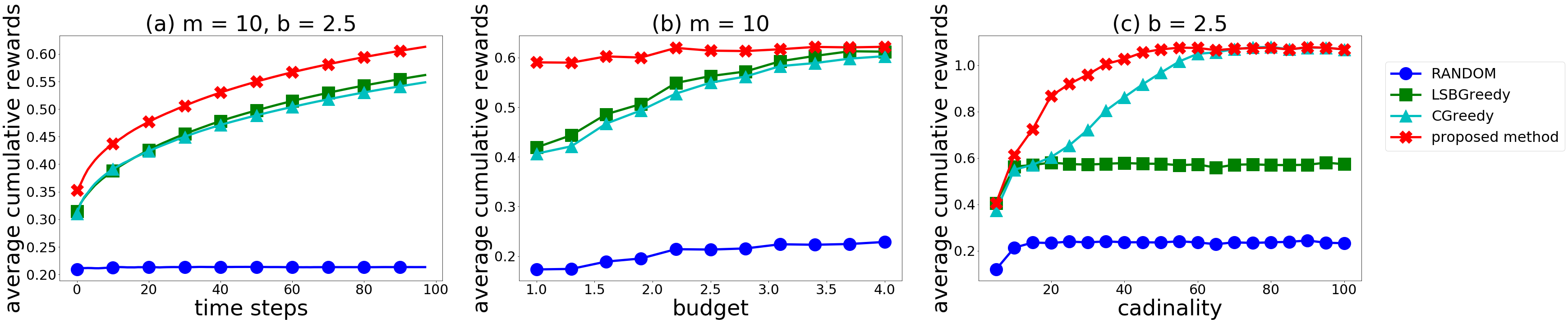
Figure 1: Cumulative average rewards on the synthetic news article recommendation dataset

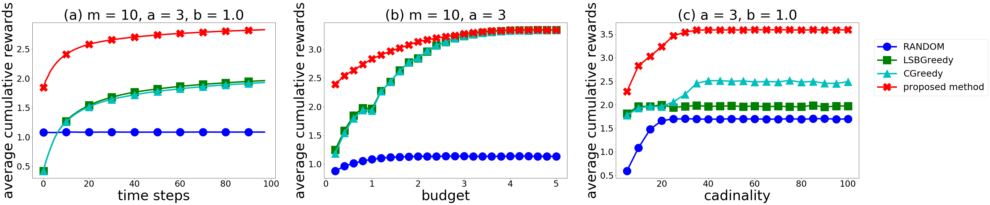
Figure 2: Cumulative average rewards on the MovieLens dataset

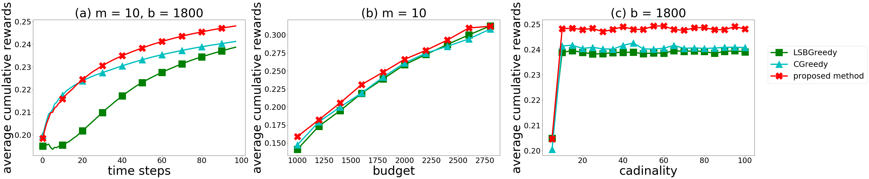
Figure 3: Cumulative average rewards on the Million Song Dataset

In this section, we empirically evaluate our methods by a synthetic dataset that simulates an environment for news article recommendation and two real-world datasets (MovieLens100K [Grouplens, 1998] and the Million Song Dataset [Bertin-Mahieux et al., 2011]).

We compare our proposed algorithm to the following baselines:

• RANDOM. In each round, this algorithm selects elements uniform randomly until no element satisfies the constraints.

• LSBGreedy. This was proposed in [Yue and Guestrin, 2011] to solve the submodular bandit problem under a cardinality constraint. In the linear kernel case, SM-UCB [Chen et al., 2017] is equivalent to LSBGreedy.

• CGreedy. This is an algorithm for a submodular bandit problem under a knapsack constraint and was proposed in [Yu et al., 2016]. They also proposed an algorithm called MCSGreedy. However because MCSGreedy is computationally expensive (in each round it calls functions $f_{1},\dots,f_{d}$ for $O(|\mathcal{N}|^{3})$ times) and their experimental results show that both algorithms have a similar empirical performance, we do not add MCSGreedy to the baselines.

In Proposition 2, we showed that these greedy algorithms incur linear approximation regret in the worst case. However, even without theoretical guarantee, it is empirically known that a greedy algorithm achieve a good experimental performance. In this section, we demonstrate that our algorithm outperforms these greedy algorithms under various combinations of constraints. As a special case, such constraints include the case when there is a sufficiently large budget for knapsack constraints and the case when the $k$-system constraint is sufficiently mild. The greedy algorithms are algorithms for such cases. We also show that our proposed method performs no worse than the baselines even in these cases.

As in the preceding work [Yue and Guestrin, 2011], we assume the score function $f$ is a linear combination of known probabilistic coverage functions. We assume there exists a set of topics (or genres) $\mathcal{G}$ with $|\mathcal{G}|=d$ and for each item $e\in\mathcal{N}$, there is a feature vector $x(e):=(P_{g}(e))_{g\in\mathcal{G}}\in\mathbb{R}^{d}$ that represents the information coverage on different genres. For each genre $g$, we define the probabilistic coverage function $f_{g}(S)$ by $1-\prod_{e\in S}(1-P_{g}(e))$ and we assume $f=\sum_{i}w_{i}f_{i}$ with unknown linear coefficients $w_{i}$. The vector $w:=[w_{1},\dots,w_{d}]$ represents user preference on genres. We assume that the noisy rewards $y_{t}^{(i)}$ are sampled by $y_{t}^{(i)}\sim\mathrm{Ber}\left(\Delta f(e_{t}^{(i)}\mid S_{t}^{(1:i-1)})\right)$. Below, we define these feature vectors $x(e)$, $w$, and constraints explicitly. We note that in the experiments, we use an un-normalized knapsack constraint $c(S)\leq b$. In the following experiments, using 100 users (100 vectors $w$), we compute cumulative average rewards for each algorithm. When taking the average, we repeated this experiment 10 times for each user.

7.1 NEWS ARTICLE RECOMMENDATION

In this synthetic dataset, we assume $d=15$ and $|\mathcal{N}|=1000$. We define $x(e)$ and costs for a knapsack constraint in a similar manner in [Yu et al., 2016]. We sample each entry of $x(e)$ from two types of uniform distributions. We assume that for each item $e$, the number of genres that have high information coverage is limited to two. More precisely, we randomly select two indices of $x(e)$ and sample entries from $U(0.5,0.8)$ and sample other entries from $U(0.0,0.01)$. We generate 100 user preference vectors $w$ in a similar way to $x(e)$. We also sample the costs of items uniform randomly from $U(0.0,1.0)$. In this dataset, we consider the intersection of a cardinality constraint and a knapsack constraint. The result is shown in Figure 1.

7.2 MOVIE RECOMMENDATION

We perform a similar experiment in [Mirzasoleiman et al., 2016] but with a semi-bandit feedback. In MovieLens100K, there are 943 users and 1682 movies. We take $\mathcal{N}$ as the set of 1682 movies in the dataset. There are $d=18$ genres in this dataset. First, we fill the ratings for all the user-item pairs using matrix factorization [Koren et al., 2009] and we normalized the ratings $r$ so that $r\in[0,1]$. For each movie $e\in\mathcal{N}$, we denote by $r_{e}\in[0,1]$ the mean of the ratings of the movie for all users. We define $P(g\mid e)=r_{e}/|\mathcal{G}_{e}|$ if $g\in\mathcal{G}_{e}$, otherwise we define $P(g\mid e)=0$. We normalize $P(g\mid e)$ as previously mentioned, because if $w_{i}=1$ for all $i$, then we have $P(\{e\})=r_{e}$.

We define a similar knapsack, cardinality, and matroid constraints to those of [Mirzasoleiman et al., 2016]. For $e\in\mathcal{N}$, the cost $c(e)$ is defined as $c(e)=F_{\mathrm{Beta}(10,2)}(r_{e})$, where $F_{\mathrm{Beta}(10,2)}$ is the cumulative distribution function of the $\mathrm{Beta}(10,2)$. For a budget $b\in\mathbb{R}_{>0}$, we consider a knapsack constraint $c(S)\leq b$. The beta distribution lets us differentiate the highly rated movies from those with lower ratings [Mirzasoleiman et al., 2016]. We generate 100 user preference vectors $w$ in a similar way to the news article recommendation example. In this dataset, we consider the following constraints on genres in addition to the knapsack $c(S)\leq b$ and cardinality $|S|\leq m$ constraints, There are $k$ genres in MovieLens100K, where $k=d=18$. For each genre $g$, we fix a non-negative integer $a$ and consider the constraint $|\left\{e\in S\mid e\text{ has genre }g\right\}|\leq a$ for $S\subseteq\mathcal{N}$. This can be regarded as a partition matroid constraint. Therefore, the intersection of the constraints for all genres is a $k$-system constraint. One can prove that the intersection of this $k$-system constraint and a cardinality constraint is also a $k$-system constraint. The results are displayed in Figure 2 in the case of the matroid limit $a=3$.

7.3 MUSIC RECOMMENDATION

From the Million Song Dataset, we select 1000 most popular songs and 30 most popular genres. Thus, we have $|\mathcal{N}|=1000$ and $d=30$. For active 100 users, we compute $P_{g}(e)$ and user preference vector $w$ in almost the same way as $\overline{w}(e,g)$ and $\theta^{*}$ in [Hiranandani et al., 2019] respectively. They assume that a user likes a song $e$ if the user listened to the song at least five times, however, we assume that a user likes the song if the user listened to the song at least two times. We consider the intersection of a cardinality and a knapsack constraint $c(S)\leq b$. We define a cost $c$ for the knapsack constraint by the length (in seconds) of the song in the dataset. The costs represent the length of time spent by users before they decide to listen to the song and we assume that it is proportional to the length of the song . The results are displayed in Figure 3. We do not show the performance of RANDOM in the figure since it achieves only very low rewards.

7.4 RESULTS

In Figures 1a, 2a, 3a, we plot the cumulative average rewards for each algorithm up to time step $T=100$. In Figures 1b, 2b, and, 3b (resp. 1c, 2c, and, 3c), we show the cumulative average rewards at the final round by changing the budget $b$ (resp. by changing the cardinality limit $m$) and fixing the cardinality limit $m$ (resp. fixing the budget $b$). These results shows that overall our proposed method outperforms the baselines. We note that Figure 3 shows different tendency as compared to other datasets since popular items in the Million Song Dataset have high information coverage for multiple genres and about 47 $\%$ of the items have low information coverage (less than 0.01) for all genres. Figures 1b, 2b, and 3b also show the results for the case when the budget is sufficiently large. This is the case when LSBGreedy performs well and our experimental results show that even in this case, our method have comparable performance to greedy algorithms. Moreover, Figures 1c, 2c, and 3c also show the results in the case when the cardinality constraints are sufficiently mild. In this case, CGreedy performs well since the constraints are almost same as a knapsack constraint. The experimental results show that our method tends to have better performance than that of CGreedy even in this case.

8 CONCLUSIONS

In this study, motivated by diversified retrieval considering cost of items, we introduced the submodular bandit problem under the intersection of a $k$-system and knapsack constraints. Then, we proposed a non-greedy algorithm to solve the problem and provide a strong theoretical guarantee. We demonstrated our proposed method outperforms the greedy baselines using synthetic and two real-world datasets.

A possible generalization of this work is a generalization to the full bandit setting. In this setting, a leaner observes only a value $f(S_{t})+\epsilon$ in each round. Since it needs much work to derive a theoretical guarantee, we leave this setting for future work.

APPENDIX

In this appendix, we generalize the reward model considered in the main article to the kernelized setting as in [Chen et al., 2017]. We also provide parameters used in the experiments.

9 PROBLEM FORMULATION UNDER A GENERALIZED REWARD MODEL

In this appendix, we consider the same reward model as in [Chen et al., 2017], but subject to the intersection of knapsacks and $k$-system constraint as in the main article. SM-UCB [Chen et al., 2017] is based on CGP-UCB [Krause and Ong, 2011] or GP-UCB [Srinivas et al., 2010]. However, recently, [Chowdhury and Gopalan, 2017] improved the assumption and the regret analysis of GP-UCB [Srinivas et al., 2010]. We follow setting of [Chowdhury and Gopalan, 2017].

Let $\Phi$ be a compact subset of some Euclidean space, which represents the space of contexts. We consider the following sequential decision making process for times steps $t=1,\dots,T$.

1. The algorithm observes context $\phi_{t}\in\Phi$ and selects a list $S_{t}=\left\{e^{(1)}_{t},\dots,e^{(m_{t})}_{t}\right\}\subseteq\mathcal{N}$ satisfying the constraints.

2. The algorithm receives noisy rewards $y_{t}^{(1)},\dots,y_{t}^{(m_{t})}$ as follows:

   $$y_{t}^{(i)}=\Delta f_{\phi_{t}}\left(e_{t}^{(i)}\mid S_{t}^{(1:i-1)}\right)+\varepsilon_{t}^{(i)},$$

   for $i=1,\dots,m_{t}$. Here $f_{\phi_{t}}$ is a non-negative, monotone submodular function unknown to the algorithm, $S_{t}^{(1:i-1)}=\left\{e_{t}^{(1)},\dots,e_{t}^{(i-1)}\right\}$ and $\varepsilon_{t}^{(i)}$ is a noise.

Here, we regard $\phi_{t},S_{t}^{(1:i-1)}$, $e_{t}^{(i-1)}$ and $\varepsilon_{t}^{(i)}$ as random variables.

9.1 ASSUMPTIONS REGARDING THE SCORE FUNCTION $f_{\phi}$

The linear model considered in the main article can be generalized to an infinite dimensional case [Chen et al., 2017]. We let $D:=\Phi\times 2^{\mathcal{N}}\times\mathcal{N}$ and define $\chi:D\rightarrow\mathbb{R}$ by $\chi((\phi,S,e))=\Delta f_{\phi}(e\mid S)$. We assume that there exists an RKHS (reproducing kernel Hilbert space) $\mathcal{H}$ on $D$ with a positive definite (or linear) kernel $\kappa$ and $\chi$ belongs to $\mathcal{H}$ and the norm $|\chi|_{\mathcal{H}}$ is bounded by $B>0$. We assume that $\kappa$ is continuos on $D\times D$. We also assume that $\kappa(x,x)\leq 1$ for any $x\in D$. If $\kappa(x,x)\leq c$, then our $\alpha$-regret would increase by a factor of $\sqrt{c}$.

9.2 ASSUMPTIONS REGARDING NOISE STOCHASTIC PROCESS

As for noises, we consider the same assumption as in the main article.

10 DEFINITION OF UCB SCORES

In this section, following [Chen et al., 2017, Chowdhury and Gopalan, 2017], we generalize UCB scores defined in the main article.

We let $x_{t}^{(i)}=(\phi_{t},\allowbreak S_{t}^{(1:i-1)},\allowbreak e_{t}^{(i)})\in D$ and $\mathbf{x}_{(1:t)}=(x_{1}^{(1)},\allowbreak\dots,\allowbreak x_{1}^{(m_{1})},\allowbreak\dots,\allowbreak x_{t}^{(1)},\allowbreak\dots x_{t}^{(m_{t})})\in D^{M}$, where $M=\sum_{s=1}^{t}m_{s}$. We also define $\mathbf{y}_{(1:t)}\in\mathbb{R}^{M}$ as $(y_{1}^{(1)},\allowbreak\dots,\allowbreak y_{1}^{(m_{1})},\allowbreak\dots,\allowbreak y_{t}^{(1)},\allowbreak\dots y_{t}^{(m_{t})})$. For a sequence $\xi=(\xi_{1},\dots,\xi_{s})\in D^{s}$, we define $K(\xi)=\left(\kappa(\xi_{i},\xi_{j})\right)_{1\leq i,j\leq s}\in\mathbb{R}^{s\times s}$ and $\kappa(\xi,x)=[\kappa(\xi_{1},x),\dots,\kappa(\xi_{s},x)]^{\mathrm{T}}\in\mathbb{R}^{s}$. We also let $\kappa_{t}(x)=\kappa(\mathbf{x}_{(1:t)},x)\in\mathbb{R}^{M}$ and $K_{t}=K(\mathbf{x}_{(1:t)})\in\mathbb{R}^{M\times M}$. Then, we define $\mu_{t}(x)\in\mathbb{R}$ and $\sigma_{t}^{2}(x)\in\mathbb{R}_{>0}$ as follows:

$$\mu_{t}(x) =\kappa_{t}(x)^{\mathrm{T}}\left(K_{t}+\lambda I\right)^{-1}\mathbf{y}_{1:t},$$

$$\kappa_{t}(x,x^{\prime}) =\kappa(x,x^{\prime})-\kappa_{t}(x)^{\mathrm{T}}\left(K_{t}+\lambda I\right)^{-1}\kappa_{t}(x^{\prime}),$$

$$\sigma_{t}^{2}(x) =\kappa_{t}(x,x).$$

Here, $\lambda\in\mathbb{R}_{>0}$ is a parameter of the model. If $x=(\phi,S,e)$, we also write $\mu_{t}(e\mid\phi,S)=\mu_{t}(x)$ and $\sigma_{t}(e\mid\phi,S)=\sigma_{t}(x)$.

We define a UCB score of the marginal gain by

$$\mathrm{ucb}_{t}(e\mid\phi,S)=\mu_{t-1}(e\mid\phi,S)+\beta_{t-1}\sigma_{t-1}(e\mid\phi,S),$$

and a modified UCB score by $\mathrm{ucb}_{t}(e\mid\phi,S)/c(e)$. Here, $\beta_{t}$ is defined as $B+R\sqrt{2\left(\gamma_{M_{t}}+1+\ln(1/\delta)\right)}$ and $M_{t}=\sum_{s=1}^{t}m_{s}$. Here $\gamma_{s}$ is the maximum information gain [Srinivas et al., 2010, Chowdhury and Gopalan, 2017] after observing $s$ rewards. We refer to [Chowdhury and Gopalan, 2017] for the definition.

The following proposition is a generalization of Proposition 1 and is a direct consequence of (the proof of) [Chowdhury and Gopalan, 2017, Theorem 2].

Proposition 4.

We assume there exists $m\in\mathbb{Z}_{\geq 1}$ such that $m_{t}\leq m$ for all $1\ \leq t\leq T$. Then, with probability at least $1-\delta$, the following inequality holds:

$$\left|\mu_{t-1}(e\mid\phi,S)-\Delta f_{\phi}(e\mid S)\right|\leq\beta_{t-1}\sigma_{t-1}(e\mid\phi,S),$$

for any $t,\phi,S,$ and $e$.

11 STATEMENT OF THE MAIN THEOREM

With generalized UCB scores, we consider the same algorithm in the main article. Then, we provide a statement for the generalized version of Theorem 1.

Theorem 2.

Let the notation and assumptions be as previously mentioned. We also assume that $\lambda\geq m$. We let $\alpha=\frac{1}{(1+\varepsilon)\left(k+2l+1\right)}$, and define $\alpha$-regret as

$$\mathrm{Reg}_{\alpha}\left(T\right)=\sum_{t=1}^{T}\alpha f_{\phi_{t}}(OPT_{t})-f_{\phi_{t}}(S_{t}),$$

where $OPT_{t}$ is a feasible optimal solution at round $t$. Then, with probability at least $1-\delta$, the proposed algorithm achieves the following $\alpha$-regret bound:

$$\mathrm{Reg}_{\alpha}\left(T\right)\leq 8\beta_{T}\sqrt{mT\gamma_{mT}}.$$

In particular, with at least probability $1-\delta$, the $\alpha$-regret $\mathrm{Reg}_{\alpha}\left(T\right)$ is given as

$$O\left(B\sqrt{T^{\prime}\gamma_{T^{\prime}}}+R\sqrt{T^{\prime}\gamma_{T^{\prime}}\left(\gamma_{T^{\prime}}+1+\ln(1/\delta)\right)}\right),$$

where $T^{\prime}=mT$.

Remark 2.

1. The maximum information gain $\gamma_{T}$ is $O(d\ln T)$ and $O((\ln T)^{d+1})$ if the kernel is a $d$-dimensional linear and Squared Exponential kernel, respectively [Srinivas et al., 2010]. They also showed that a similar result for the Matèrn kernel. Thus, if the kernel is a $d$-dimensional kernel, up to a polylogarithmic factor, we obtain Theorem 1 in the main article as a corollary.

2. In the main article, we assume that the norm of vector $[\Delta f_{i}(e\mid S)]_{i=1}^{d}$ is bounded above by $A$. Moreover, the factor $A$ appears in the regret bound in Theorem 1. However, since we normalize the kernel so that $\kappa(x,x)\leq 1$, a factor corresponding to $A$ does not appear in Theorem 2.

12 PROOF OF THE MAIN THEOREM

Throughout the proof, we assume that assumptions of Proposition 4 hold and fix the event $\mathcal{F}$ on which the inequality in Proposition 4 holds.

12.1 GREEDY ALGORITHM UNDER A $k$-SYSTEM CONSTRAINT

In this subsection, we fix time step $t$ and context $\phi$ and consider the greedy algorithm under only $k$-system constraint as shown in Algorithm 3. Here, we drop $\phi$ from notation. We denote by $(\mathcal{N},\mathcal{I})$ the $k$-system.

$S=\emptyset$

while True do

       $\mathcal{N}^{\prime}=\left\{e\in\mathcal{N}\mid S+e\in\mathcal{I}\right\}$

       if $\mathcal{N}^{\prime}\neq\emptyset$ then

             $e=\operatorname{argmax}_{e\in\mathcal{N}^{\prime}}\mathrm{ucb}_{t}(e\mid\phi,S)$

             Add $e$ to $S$

            

      else

             break

            

       end if

      

end while

Return $S$

Algorithm 3 GREEDY UCB

Proposition 5.

Let $S$ be a set returned by Algorithm 3. Then for any feasible set $C$, on the event $\mathcal{F}$, the following inequality holds:

$$f(S)+\frac{2k\beta_{t-1}}{k+1}\sigma_{t-1}(S)\geq\frac{1}{k+1}f(S\cup C).$$

Proof.

This can be proved in a similar way to the proof in [Calinescu et al., 2011, Appendix B]. We note the proof given in Appendix B works even if we replace the optimal solution $O$ by any feasible set $C$. We write $S=\left\{e_{1},\dots,e_{m}\right\}$, where $e_{1},\dots,e_{m}$ are added by Algorithm 3 with this order. We construct a partition $C_{1},\dots,C_{m}$ of $C$ in the same way to the construction of $O_{i}$ in [Calinescu et al., 2011]. Then $|C_{i}|\leq k$ for any $i$ and $S^{(1:i-1)}+e$ is feasible for any $e\in C_{i}$. By the choice of the greedy algorithm and Proposition 4, with probability at least $1-\delta$, we have

$$\Delta f(e\mid S^{(1:i-1)})$$

$$\leq\mu_{t-1}(e\mid S^{(1:i-1)})+\beta_{t-1}\sigma_{t-1}(e\mid S^{(1:i-1)})$$

$$\leq\mu_{t-1}(e_{i}\mid S^{(1:i-1)})+\beta_{t-1}\sigma_{t-1}(e_{i}\mid S^{(1:i-1)})$$

$$\leq\Delta f(e_{i}\mid S^{(1:i-1)})+2\beta_{t-1}\sigma_{t-1}(e_{i}\mid S^{(1:i-1)}),$$

for any $i$ and any $e\in C_{i}$. Here we use Proposition 4 in the first and third inequality. The second inequality follows from the choice of the greedy algorithm and the fact that $S^{(1:i-1)}+e$ is feasible. Noting that $|C_{i}|\leq k$ and taking the sum of both sides for $e\in C_{i}$, we have

$$k\left(\Delta f(e_{i}\mid S^{(1:i-1)})+2\beta_{t-1}\sigma_{t-1}(e_{i}\mid S^{(1:i-1)})\right)$$

$$\geq\sum_{e\in C_{i}}\Delta f(e\mid S^{(1:i-1)})$$

$$\geq\Delta f(C_{i}\mid S^{(1:i-1)})\geq\Delta f(C_{i}\mid S).$$

Here for subsets $A,B\in\mathcal{N}$, we define $\Delta f(A\mid B)=f(A\cup B)-f(B)$ and in the second and third inequality, we use the submodularity. By taking the sum of both sides, we have

$$k\left(f(S)-f(\emptyset)+2\beta_{t-1}\sum_{i=1}^{m}\sigma_{t-1}(e_{i}\mid S^{(1:i-1)})\right)$$

$$\geq\sum_{i=1}^{m}\Delta f(C_{i}\mid S)\geq\Delta f(C\mid S)=f(C\cup S)-f(S).$$

Here the second inequality follows from submodularity of $f$. Thus by non-negativity of $f$, we have our assertion. ∎

12.2 SOLUTIONS OF AFSM-UCB AT EACH ROUND

In this subsection, we assume that assumptions of Theorem 2 are satisfied. The objective in this subsection is to provide a lower bound of the score of the set returned by AFSM-UCB at each round. In this subsection, we also fix time step $t$.

In the next proposition, we consider sets returned by GM-UCB.

Proposition 6.

Let $C\subseteq\mathcal{N}$ be any set satisfying knapsack and $k$-system constraints. Let $S$ be a set returned by GM-UCB. Then with probability at least $1-\delta$, we have

$$f(S)+2\beta_{t-1}\sigma_{t-1}(S)\geq\min\left\{\frac{\rho}{2},\frac{1}{k+1}f(S\cup C)-\frac{l\rho}{k+1}\right\}.$$

Proof.

This can be proved in a similar way to the proof of [Badanidiyuru and Vondrák, 2014, Theorem 6.1] or [Mirzasoleiman et al., 2016, Theorem 5.1]. However, because of uncertainty, we need further analysis. We divide the proof into two cases.

Case One. This is the case when GM-UCB terminates because there exists an element $e$ such that $\mathrm{ucb}_{t}(e\mid S)\geq\rho c(e)$ and $\mathrm{ucb}_{t}(e\mid\emptyset)\geq\rho c(e)$, but any element $e$ satisfying $\mathrm{ucb}_{t}(e\mid S),\mathrm{ucb}_{t}(e\mid\emptyset)\geq\rho c(e)$ does not satisfy the knapsack constraints, i.e., $c_{j}(S+e)>1$ for some $1\leq j\leq l$. We fix an element $e^{\prime}$ satisfying $\mathrm{ucb}_{t}(e^{\prime}\mid S),\mathrm{ucb}_{t}(e^{\prime}\mid\emptyset)\geq\rho c(e^{\prime})$. We write $S=\left\{e_{1},\dots,e_{m}\right\}$. Then by assumption, for any $i$, we have $\mathrm{ucb}_{t}(e_{i}\mid S^{(1:i-1)})\geq\rho c(e_{i})$. By Proposition 4, on the event $\mathcal{F}$, we have $\Delta f(e_{i}\mid S^{(1:i-1)})+2\beta_{t-1}\sigma_{t-1}(e_{i}\mid S^{(1:i-1)})\geq\rho c(e_{i})$ for any $t,i$. By summing the both sides, we obtain

$$f(S)+2\beta_{t-1}\sigma_{t-1}(S)\geq\rho c(S).$$

On the event $\mathcal{F}$, we also have

$$f(S)+2\beta_{t-1}\sigma_{t-1}(S)\geq$$

$$\quad\mathrm{ucb}_{t}(e_{1}\mid\emptyset)\geq\mathrm{ucb}_{t}(e^{\prime}\mid\emptyset)\geq\rho c(e^{\prime}).$$

Therefore, we have

$$f(S)+2\beta_{t-1}\sigma_{t-1}(S)\geq\rho\max\left\{c(S),c(e^{\prime})\right\}\geq\frac{\rho}{2}\left(c(S)+c(e^{\prime})\right)$$

$$=\frac{\rho}{2}\sum_{j}\left(c_{j}(S)+c_{j}(e^{\prime})\right)\geq\frac{\rho}{2}.$$

Here the last inequality holds because $S+e^{\prime}$ does not satisfy the knapsack constraints.

Case Two. This is the case when GM-UCB terminates because for any element $e$ satisfying $\mathrm{ucb}_{t}(e\mid S),\mathrm{ucb}_{t}(e\mid\emptyset)\geq\rho c(e)$, $e$ satisfies knapsack constraints but $S+e$ does not satisfies the $k$-system constraint. We note that this case includes the case when there does not exist an element $e$ satisfying $\mathrm{ucb}_{t}(e\mid S),\mathrm{ucb}_{t}(e\mid\emptyset)\geq\rho c(e)$.

We divide $C$ into two sets $C_{<\rho}$ and $C_{\geq\rho}$, that is, we define

$$C_{<\rho} =\left\{e\in C\mid\exists i\text{ such that }\mathrm{ucb}_{t}(e\mid S^{(1:i)})<\rho c(e)\right\},$$

$$C_{\geq\rho} =C\setminus C_{<\rho}$$

$$=\left\{e\in C\mid\forall i\quad\mathrm{ucb}_{t}(e\mid S^{(1:i)})\geq\rho c(e)\right\}.$$

Let $e\in C_{<\rho}$. Then on the event $\mathcal{F}$, we have $\Delta f(e\mid S)\leq\Delta f(e\mid S^{(1:i)})\leq\mathrm{ucb}_{t}(e\mid S^{(1:i)})<\rho c(e)$ for some $i$. Here the first inequality follows from submodularity and the second inequality follows from Proposition 4. Therefore, the following inequality holds:

$$\Delta f(C_{<\rho}\mid S)\leq\sum_{e\in C_{<\rho}}\Delta f(e\mid S)\leq\sum_{e\in C_{<\rho}}\rho c(e)\leq l\rho.$$ (3)

Here the first inequality follows from the submodularity of $f$ and the second inequality follows from the fact that $C_{<\rho}$ is a feasible set.

Next, we consider $C_{\geq\rho}$. We run Algorithm 3 on $S\cup C_{\geq\rho}$. By assumption of this case, Algorithm 3 returns $S$. Proposition 5 implies that $f(S)+2\beta_{t-1}\sigma_{t-1}(S)\geq\frac{1}{k+1}f(S\cup C_{\geq\rho}).$ Rewriting, we have

$$\Delta f(C_{\geq\rho}\mid S)\leq kf(S)+2(k+1)\beta_{t-1}\sigma_{t-1}(S).$$

By this, equation (2), and submodularity of $f$, we have

$$\Delta f(C\mid S)\leq\Delta f(C_{<\rho}\mid S)+\Delta f(C_{\geq\rho}\mid S)$$

$$\leq l\rho+kf(S)+2(k+1)\beta_{t-1}\sigma_{t-1}(S).$$

Noting that $\Delta f(C\mid S)=f(C\cup S)-f(S)$, we have

$$f(S)+2\beta_{t-1}\sigma_{t-1}(S)\geq\frac{1}{k+1}f(S\cup C)-\frac{l\rho}{k+1}.$$

This completes the proof. ∎

The following is a key lemma for the proof of our main Theorem.

Lemma 1.

Let $\alpha=\frac{1}{(1+\varepsilon)\left(k+2l+1\right)}$. Let $S$ be the set returned by AFSM-UCB and $OPT$ the optimal feasible set. Then on the event $\mathcal{F}$, $S$ satisfies the following:

$$f(S)+4\beta_{t-1}\sigma_{t-1}(S)\geq\alpha f(OPT).$$

Proof.

By monotonicity and assumption, we have $\nu\leq\max_{e\in\mathcal{N}}f(\{e\})\leq f(OPT)$. Here, we note that by assumptions any singleton $\{e\}$ for $e\in\mathcal{N}$ is a feasible set. By submodularity of $f$ and the assumption of $\nu^{\prime}$, we have

$$f(OPT)\leq\sum_{e\in OPT}f(\{e\})\leq|OPT|\nu^{\prime}\leq|\mathcal{N}|\nu^{\prime}.$$

We put $r=\frac{2}{k+2l+1}$ and $r_{OPT}=rf(OPT)$. By bounds of $f(OPT)$ above, there exists $\rho$ in the while loop in AFSM-UCB such that $(1+\varepsilon)^{-1}r_{OPT}\leq\rho\leq r_{OPT}$. We denote such a $\rho$ by $\rho^{*}$. Moreover, if $\rho=r_{OPT}$, then we have $\rho/2=\frac{1}{k+1}f(OPT)-\frac{l\rho}{k+1}$. By Proposition 6, on the event $\mathcal{F}$, we have

$$\mu_{t-1}(S_{\rho^{*}})+3\beta_{t-1}\sigma_{t-1}(S_{\rho^{*}})\geq f(S_{\rho^{*}})+2\beta_{t-1}\sigma_{t-1}(S_{\rho^{*}})\geq\frac{r_{OPT}}{2(1+\varepsilon)}=\alpha f(OPT).$$

Here we denote by $S_{\rho}$ the returned set of GM-UCB with threshold $\rho$. Because AFSM-UCB returns a set with the largest UCB score in $\{S_{\rho}\}_{\rho}$, we have our assertion. ∎

Remark 3.

Suppose that the cardinality of any feasible solution is bounded by $m\in\mathbb{Z}_{>0}$. Then, by the proof of Lemma 1, we see that in AFSM-UCB, the condition in the while loop $\rho\leq r\nu^{\prime}|\mathcal{N}|$ can be replaced to $\rho\leq r\nu^{\prime}m$. We obtain the same theoretical guarantee for this modified algorithm. Following FANTOM [Mirzasoleiman et al., 2016], we use the condition $\rho\leq r\nu^{\prime}|\mathcal{N}|$.

12.3 PROOF OF THE MAIN THEOREM

In this subsection, first, we introduce a lemma similar to [Chowdhury and Gopalan, 2017, Lemma 4] and prove the main Theorem.

Lemma 2.

Let $S_{t}$ be the set selected by AFSM-UCB at time step $t$. We assume that $\lambda\geq m$. Then, we have

$$\sum_{t=1}^{T}\sigma_{t-1}(S_{t}\mid\phi_{t})\leq 2\sqrt{mT\gamma_{mT}}.$$

Proof.

First, suppose the kernel is a linear kernel. Then by [Yue and Guestrin, 2011, Lemma 5], the definition of $\gamma_{T}$, and monotonicity of $T\mapsto\gamma_{T}$ [Krause and Guestrin, 2005], we have $\sum_{t=1}^{T}\sigma_{t-1}^{2}(S_{t}\mid\phi_{t})\leq 4\gamma_{mT}.$ And the statement of the lemma follows from this inequality and the Cauchy-Schwartz inequality. Suppose that the kernel is a positive definite. Let $\{\psi_{i}\}_{i=1}^{\infty}$ be an orthonormal basis of the RKHS. Then for $x\in D$, we have $\kappa(x,\cdot)=\sum_{i=1}^{\infty}a_{i}(x)\psi_{i}$, where $a_{i}(x)\in\mathbb{R}$. Therefore, for each $x,y\in D$, we have $\kappa(x,y)=\sum_{i=1}^{\infty}a_{i}(x)a_{i}(y)$. Since for fixed $T$, only finitely many values of $\kappa$ are appeared in the both sides of the inequality of the lemma, the statement for positive definite kernels can be proved by taking the limit of the inequality in the linear kernel case (see the proof of [Chowdhury and Gopalan, 2017, Theorem 2]). ∎

Proof of the main Theorem.

Because $t\mapsto\beta_{t}$ is non-decreasing and by Lemma 1, we see that the $\alpha$-regret is bounded by $4\beta_{T}\sum_{t=1}^{T}\sigma(S_{t}\mid\phi)$ with probability at least $1-\delta$ . Then the assertion of the main result follows from Lemma 2. We also note that the second statement in the main article follows from the proof of [Srinivas et al., 2010, Theorem 8]. ∎

Remark 4.

We consider only stationary constraints for simplicity, i.e., the constraints (1) do not depend on time step $t$. However, it is clear from the proof that only $k$ and $l$ should be stationary and we can consider non-stationary constraints.

13 PROOF OF PROPOSITION 2

In this section, we prove that MCSGreedy [Yu et al., 2016] and LSBGreedy [Yue and Guestrin, 2011] perform arbitrary poorly in some situations. We denote by $\mathrm{Reg}_{\alpha,\mathrm{MCS}}(T)$ and $\mathrm{Reg}_{\alpha,\mathrm{LSB}}(T)$ the $\alpha$-regret of MCSGreedy and LSBGreedy respectively.

Proposition 7.

For any $\alpha>0$, there exists cost $c$, $k$-system $\mathcal{I}$, a submodular function $f$, $T_{0}>0$ and a constant $C>0$ such that with probability at least $1-\delta$,

$$\mathrm{Reg}_{\alpha,\mathrm{MCS}}(T)>CT,$$

for any $T>T_{0}$. Moreover, the same statement holds for $\mathrm{Reg}_{\alpha,\mathrm{LSB}}(T)$.

Proof.

We prove the statement only for MCSGreedy. We skip the proof for LSBGreedy because it is similar and simpler. We take a $k$-system constraint as the cardinality constraint $|S|\leq m$, where we choose $m$ later. We consider $\mathcal{N}$ as the disjoint union of $\mathcal{N}_{1}$ and $\mathcal{N}_{2}$, where $|\mathcal{N}_{1}|=|\mathcal{N}_{2}|=m$. We define cost $c:\mathcal{N}\rightarrow\mathbb{R}$ as

$$c(e)=\begin{cases}\frac{1}{m}&\text{if }e\in\mathcal{N}_{1},\\ \frac{1}{m^{2}}&\text{if }e\in\mathcal{N}_{2}.\end{cases}$$

For each $e\in\mathcal{N}$, we define $v_{e}$ as follows:

$$v(e)=\begin{cases}\frac{1}{m}&\text{if }e\in\mathcal{N}_{1},\\ \frac{1+\epsilon}{m^{2}}&\text{if }e\in\mathcal{N}_{2}.\end{cases}$$

Here $\epsilon$ is a small positive number. We assume that the objective function $f:2^{\mathcal{N}}\rightarrow\mathbb{R}$ is a modular function, i.e, $f(A)=\sum_{e\in A}v(e)$ for $A\subseteq\mathcal{N}$. For $e\in\mathcal{N}$, we define a function $\chi_{e}:2^{\mathcal{N}}\rightarrow\mathbb{R}$ as

$$\chi_{e}(A)=\begin{cases}1&\text{if }e\in A,\\ 0&\text{otherwise}\end{cases}$$

Then we have $f(A)=\sum_{e\in\mathcal{N}}v(e)\chi_{e}(A)$. Therefore, this is the linear kernel case. Moreover, because feature vectors $[\chi_{e}(e^{\prime}|A)]_{e\in\mathcal{N}}$, for $e^{\prime}\not\in A$ are orthogonal, this case can be reduced to the MAB setting. Therefore, we can use the UCB in Lemma 6 [Abbasi-Yadkori et al., 2011].

Denote by $S_{t}$ the set selected by MCSGreedy and by $OPT$ the optimal solution. Because $c(e)\leq 1/m$ for all $e\in\mathcal{N}$, we have $|S_{t}|=m$. It is easy to see that $OPT=\mathcal{N}_{1}$. Therefore we have $f(OPT)=1$.

We take sufficiently large $m$ so that

$$\frac{(m-3)(1+\epsilon)}{m^{2}}+\frac{3}{m}<\alpha.$$

For $e\in\mathcal{N}$ and $1\leq t\leq T$, we denote by $N_{e,t}$ the number of times $e$ is selected in time steps $\tau=1,\dots,t$. Then by Lemma 6 [Abbasi-Yadkori et al., 2011], UCB of $v(e)$ for $e\in\mathcal{N}$ is given as $\mu_{e,t}+\sigma_{e,t}$ where $\mu_{e,t}$ is the mean of feedbacks for $v(e)$ and $\sigma_{e,t}$ is given as follows:

$$\sigma_{e,t}=\sqrt{\frac{1+N_{e,t}}{N_{e,t}^{2}}\left(1+2\ln\left(d(1+N_{e,t})^{1/2}/\delta\right)\right)},$$

where $d=2m$. We note that at each round MCSGreedy selects elements with the largest modified UCB $(\mu_{e,t}+\sigma_{e,t})/c(e)$ except the first three elements. Suppose that the modified UCB of an element in $\mathcal{N}_{1}$ is greater than that of an element in $\mathcal{N}_{2}$, that is,

$$m(\mu_{e_{1},t}+\sigma_{e_{1},t})>m^{2}(\mu_{e_{2},t}+\sigma_{e_{2},t}).$$

By Lemma 6 [Abbasi-Yadkori et al., 2011], we have with probability at least $1-\delta$,

$$m(v(e_{1})+2\sigma_{e_{1},t})\geq m(\mu_{e_{1},t}+\sigma_{e_{1},t})>m^{2}(\mu_{e_{2},t}+\sigma_{e_{2},t})\geq m^{2}v(e_{2}).$$

Thus we have

$$2m\sigma_{e_{1},t}>\epsilon.$$

Therefore, there exists $N(\delta,\epsilon,m)\in\mathbb{Z}_{>0}$ such that

$$N_{e_{1},t}<N(\delta,\epsilon,m).$$

We assume that $T$ is sufficiently large compared to $N(\delta,\epsilon,m)$. We see that MCSGreedy selects at least $(m-3)T-mN(\delta,\epsilon,m)$ elements from $\mathcal{N}_{2}$. Thus with probability at least $1-\delta$, we have

$$\sum_{t=1}^{T}f(S_{t})\leq\left((m-3)T-mN(\delta,\epsilon,m)\right)\frac{1+\epsilon}{m^{2}}+\left(3T+mN(\delta,\epsilon,m)\right)\frac{1}{m}.$$

Because

$$\alpha\sum_{t=1}^{T}f(OPT)=\alpha T,$$

we have our assertion. ∎

14 PARAMETERS IN THE EXPERIMENTS

Because this is the linear kernel case, by Theorem 5 [Srinivas et al., 2010], we have $\gamma_{t}=O(k\ln t)$. Thus we modify the definition of $\beta_{t}$ as $\beta_{t}=B+R_{1}\sqrt{R_{2}k\ln m_{t}+1+\ln(1/\delta)},$ where $B,R_{1}$, and $R_{2}$ parameters. For all datasets, we take $\nu=0.01$ and $\nu^{\prime}=1.0$. We take $\varepsilon=0.3$, $\varepsilon=1.0$, and $\varepsilon=0.1$ for the news article recommendation dataset, MovieLens100k, and the Million Song Dataset respectively. We tune other parameters by using different users. Explicitly, we take $\beta=0.01,R_{1}=0.1,R_{2}=1.0,\lambda=0.1$ for the news article recommendation example, $\beta=0.01,R_{1}=0.1,R_{2}=1.0,\lambda=1.0$ for MovieLens100k, and $\beta=0.01,R_{1}=0.01,R_{2}=1.0,\lambda=3.0$ for the Million Song Dataset.

References

- Abbasi-Yadkori et al. [2011] Yasin Abbasi-Yadkori, Dávid Pál, and Csaba Szepesvári. Improved algorithms for linear stochastic bandits. In Advances in Neural Information Processing Systems, pages 2312–2320, 2011.
- Badanidiyuru and Vondrák [2014] Ashwinkumar Badanidiyuru and Jan Vondrák. Fast algorithms for maximizing submodular functions. In Proceedings of the twenty-fifth annual ACM-SIAM symposium on Discrete algorithms, pages 1497–1514. Society for Industrial and Applied Mathematics, 2014.
- Badanidiyuru et al. [2014] Ashwinkumar Badanidiyuru, Baharan Mirzasoleiman, Amin Karbasi, and Andreas Krause. Streaming submodular maximization: Massive data summarization on the fly. In Proceedings of the 20th ACM SIGKDD international conference on Knowledge discovery and data mining, pages 671–680, 2014.
- Bertin-Mahieux et al. [2011] Thierry Bertin-Mahieux, Daniel P.W. Ellis, Brian Whitman, and Paul Lamere. The million song dataset. In Proceedings of the 12th International Conference on Music Information Retrieval (ISMIR 2011), 2011.
- Calinescu et al. [2011] Gruia Calinescu, Chandra Chekuri, Martin Pál, and Jan Vondrák. Maximizing a monotone submodular function subject to a matroid constraint. SIAM Journal on Computing, 40(6):1740–1766, 2011.
- Chekuri et al. [2010] Chandra Chekuri, Jan Vondrak, and Rico Zenklusen. Dependent randomized rounding via exchange properties of combinatorial structures. In 2010 IEEE 51st Annual Symposium on Foundations of Computer Science, pages 575–584. IEEE, 2010.
- Chekuri et al. [2014] Chandra Chekuri, Jan Vondrák, and Rico Zenklusen. Submodular function maximization via the multilinear relaxation and contention resolution schemes. SIAM Journal on Computing, 43(6):1831–1879, 2014.
- Chen et al. [2017] Lin Chen, Andreas Krause, and Amin Karbasi. Interactive submodular bandit. In Advances in Neural Information Processing Systems, pages 141–152, 2017.
- Chen et al. [2013] Wei Chen, Yajun Wang, and Yang Yuan. Combinatorial multi-armed bandit: General framework and applications. In Proceedings of the 30th International Conference on Machine Learning, pages 151–159, 2013.
- Chowdhury and Gopalan [2017] Sayak Ray Chowdhury and Aditya Gopalan. On kernelized multi-armed bandits. In Proceedings of the 34th International Conference on Machine Learning, pages 844–853, 2017. supplementary material.
- Craswell et al. [2008] Nick Craswell, Onno Zoeter, Michael Taylor, and Bill Ramsey. An experimental comparison of click position-bias models. In Proceedings of the 2008 international conference on web search and data mining, pages 87–94. ACM, 2008.
- El-Arini et al. [2009] Khalid El-Arini, Gaurav Veda, Dafna Shahaf, and Carlos Guestrin. Turning down the noise in the blogosphere. In Proceedings of the 15th ACM SIGKDD international conference on Knowledge discovery and data mining, pages 289–298. ACM, 2009.
- Grouplens [1998] Grouplens. Movielens100k dataset. 1998. URL https://grouplens.org/datasets/movielens/100k/.
- Gupta et al. [2010] Anupam Gupta, Aaron Roth, Grant Schoenebeck, and Kunal Talwar. Constrained non-monotone submodular maximization: Offline and secretary algorithms. In International Workshop on Internet and Network Economics, pages 246–257. Springer, 2010.
- Hiranandani et al. [2019] Gaurush Hiranandani, Harvineet Singh, Prakhar Gupta, Iftikhar Ahamath Burhanuddin, Zheng Wen, and Branislav Kveton. Cascading linear submodular bandits: Accounting for position bias and diversity in online learning to rank. In Proceedings of Uncertainty in AI., 2019.
- Koren et al. [2009] Yehuda Koren, Robert Bell, and Chris Volinsky. Matrix factorization techniques for recommender systems. Computer, (8):30–37, 2009.
- Krause and Golovin [2014] Andreas Krause and Daniel Golovin. Submodular function maximization., 2014. In Tractability: Practical Approaches to Hard Problems, Cambridge University Press.
- Krause and Guestrin [2005] Andreas Krause and Carlos E Guestrin. Near-optimal nonmyopic value of information in graphical models. In Proceedings of Uncertainty in AI., 2005.
- Krause and Ong [2011] Andreas Krause and Cheng S Ong. Contextual gaussian process bandit optimization. In Advances in Neural Information Processing Systems, pages 2447–2455, 2011.
- Lattimore and Szepesvári [2019] Tor Lattimore and Csaba Szepesvári. Bandit Algorithm. Cambridge University Press, Forthcoming, 2019. https://tor-lattimore.com/downloads/book/book.pdf.
- Li and Shroff [2020] Wenxin Li and Ness Shroff, Efficient Algorithms and Lower Bound for Submodular Maximization. arXiv preprint, arXiv:1804.08178v3, 2020.
- Lin and Bilmes [2011] Hui Lin and Jeff Bilmes. A class of submodular functions for document summarization. In Proceedings of the 49th Annual Meeting of the Association for Computational Linguistics: Human Language Technologies-Volume 1, pages 510–520. Association for Computational Linguistics, 2011.
- Mestre [2006] Julián Mestre. Greedy in approximation algorithms. In European Symposium on Algorithms, pages 528–539. Springer, 2006.
- Mestre [2015] Julián Mestre. On the intersection of independence systems. Operations Research Letters, 43(1):7–9, 2015.
- Mirzasoleiman et al. [2016] Baharan Mirzasoleiman, Ashwinkumar Badanidiyuru, and Amin Karbasi. Fast constrained submodular maximization: Personalized data summarization. In Proceedings of The 33rd International Conference on Machine Learning, pages 1358–1367, 2016.
- Nemhauser and Wolsey [1978] George L Nemhauser and Laurence A Wolsey. Best algorithms for approximating the maximum of a submodular set function. Mathematics of operations research, 3(3):177–188, 1978.
- Radlinski et al. [2008] Filip Radlinski, Robert Kleinberg, and Thorsten Joachims. Learning diverse rankings with multi-armed bandits. In Proceedings of the 25th International Conference on Machine Learning, pages 784–791, 2008.
- Sarpatwar et al. [2019] Kanthi K Sarpatwar, Baruch Schieber, and Hadas Shachnai. Constrained submodular maximization via greedy local search. Operations Research Letters, 47(1):1–6, 2019.
- Srinivas et al. [2010] Niranjan Srinivas, Andreas Krause, Sham Kakade, and Matthias Seeger. Gaussian process optimization in the bandit setting: no regret and experimental design. In Proceedings of the 27th International Conference on Machine Learning, pages 1015–1022. Omnipress, 2010.
- Yu et al. [2016] Baosheng Yu, Meng Fang, and Dacheng Tao. Linear submodular bandits with a knapsack constraint. In Thirtieth AAAI Conference on Artificial Intelligence, 2016.
- Yue and Guestrin [2011] Yisong Yue and Carlos Guestrin. Linear submodular bandits and their application to diversified retrieval. In Advances in Neural Information Processing Systems, pages 2483–2491, 2011.
- Ziegler et al. [2005] Cai-Nicolas Ziegler, Sean M McNee, Joseph A Konstan, and Georg Lausen. Improving recommendation lists through topic diversification. In Proceedings of the 14th international conference on World Wide Web, pages 22–32. ACM, 2005.