A Unified Feature Representation for Lexical Connotations

Abstract

Ideological attitudes and stance are often expressed through subtle meanings of words and phrases. Understanding these connotations is critical to recognizing the cultural and emotional perspectives of the speaker. In this paper, we use distant labeling to create a new lexical resource representing connotation aspects for nouns and adjectives. Our analysis shows that it aligns well with human judgments. Additionally, we present a method for creating lexical representations that capture connotations within the embedding space and show that using the embeddings provides a statistically significant improvement on the task of stance detection when data is limited.

1 Introduction

Expressions of ideological attitudes are widespread in today’s online world, influencing how we perceive and react to events and people on a daily basis. These attitudes are often expressed through subtle expressions or associations (Somasundaran and Wiebe, 2010; Murakami and Putra, 2010). For example, the sentence “the people opposed gun control” conveys no information about the author’s opinion. However, by adding just one word, “the selfish people opposed gun control”, the author can convey their stance on both gun control (against) and the people who support it (not valuable and disliked). Discerning such subtle meaning is crucial for fully understanding and recognizing the hidden influences behind everyday content.

Recent studies in NLP have begun to examine these hidden influences through framing in social media and news (Asur and Huberman, 2010; Hartmann et al., 2019; Klenner, 2017) and style detection in hyperpartisan news (Potthast et al., 2018). Lexical connotations provide a method to study these influences, including stance, in more detail.

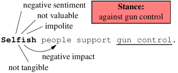
Figure 1: Connotations of the word “selfish” and the resulting implied stance on the topic “gun control”.

Connotations are implied cultural and emotional associations for words that augment their literal meanings  (Carpuat, 2015; Feng et al., 2011). Connotation values are associated with a phrase (e.g., fear is associated with “cancer”) (Feng et al., 2011) and capture a range of nuances, such as whether a phrase is an insult or implies value (see Figure 1).

In this paper, we define six new fine-grained connotation aspects for nouns and adjectives, filling a gap in the literature on connotation lexica, which has focused on verbs  (Sap et al., 2017; Rashkin et al., 2016, 2017), and coarse-grained polarity  (Feng et al., 2011; Kang et al., 2014). We create a new distantly labeled English lexicon that maps nouns and adjectives to our six aspects and show that it aligns well with human judgments. In addition, we show that our lexicon confirms existing hypotheses about subtle semantic differences between synonyms.

We then learn a single connotation embedding space for words from all parts of speech, combining our lexicon with existing verb lexica and contributing to the literature on unifying lexica (Hoyle et al., 2019). Intrinsic evaluation shows that our embedding space captures clusters of connotatively-similar words. In addition, our embedding model can generate representations for new words without the numerous training examples required by standard word-embedding methods. Finally, we show that our connotation embeddings improve performance on stance detection, particularly in a low-resource setting.

Our contributions are as follows: (1) we create a new connotation lexicon and show that it aligns well with human judgments, (2) we train a connotation feature embedding for all parts of speech and show that it captures connotations within the embedding space, and (3) we show the connotation embeddings improve stance detection when data is limited. Our resources are available: https://github.com/emilyallaway/connotation-embedding.

2 Related Work

Studies of connotation build upon the literature examining subtle language nuances, including good and bad effects of verbs (Choi and Wiebe, 2014), evoked sentiments and emotions (Mohammad et al., 2013a; Mohammad and Turney, 2010; Mohammad, 2018b), multi-dimensional sentiment (Whissell, 2009; Mohammad, 2018a; Whissell, 1989), offensiveness (Klenner et al., 2018), and psycho-sociological properties of words (Stone and Hunt, 1963; Tausczik and Pennebaker, 2009). Work explicitly on connotations has focused primarily on detailed aspects for verbs (Rashkin et al., 2016, 2017; Sap et al., 2017; Klenner, 2017) or single polarities for many parts of speech Feng et al. (2011, 2013); Kang et al. (2014). One exception is the work of  Field et al. (2019), which extends limited detailed connotation dimensions from verbs to nouns within the context of certain verbs. Our work is unique in directly defining detailed aspects for nouns and adjectives.

Early work on stance detection applied topic-specific models to various genres, including online debate forums (Sridhar et al., 2015; Somasundaran and Wiebe, 2010; Murakami and Putra, 2010; Hasan and Ng, 2013, 2014) and student essays (Faulkner, 2014). More recent studies have used a single model for many topics to predict stance in Tweets (Mohammad et al., 2016; Augenstein et al., 2016; Xu et al., 2018) and as part of the fact extraction and verification pipeline (Conforti et al., 2018; Ghanem et al., 2018; Riedel et al., 2017; Hanselowski et al., 2018). Klenner et al. (2017) explore the relationship between connotations and stance through verb frames. In contrast, our work studies stance using connotation representations from a learned joint embedding space for words from all parts of speech. Recently, Webson et al. (2020) examine representations of political ideology as connotations and its use in information retrieval. Representation learning has been used for stance detection of online debates by Li et al. (2018), who develop a joint representation of the text and the authors. Our work, however, uses a representation of word connotations and does not use any author information (a strong feature in fully-supervised datasets but which may not be available in real-world settings).

3 Connotation Lexicon

We build a connotation lexicon for nouns and adjectives by defining six new aspects of connotation. We take inspiration from verb connotation frames and their extensions (Rashkin et al., 2016; Sap et al., 2017), which define aspects of connotation in terms of the agent and theme of transitive verbs. Rashkin et al. (2016) define six aspects of connotation for verbs (entities’, writer’s, and reader’s perspectives, effect, value, and mental state) in connotation frames (e.g., “suffer” $\leadsto$ negative effect on the agent) and Sap et al. (2017) extend these aspects to include power and agency.

We first define the six new aspects of connotation for nouns and adjectives (§3.1) in our work, then we describe our distant labeling procedure (§3.2) and human evaluation of the final lexicon (§3.3).

3.1 Definitions

We use $w$ to indicate a word and $w^{\prime}$ to indicate the person, thing or attribute signified by $w$.

For each $w$, we define (1) Social Value: whether $w^{\prime}$ is considered valuable by society, (2) Politeness (Polite): whether $w$ is a socially polite term, (3) Impact whether $w^{\prime}$ has an impact on society (or the thing modified by $w$ if $w$ is an adjective), (4) Factuality (Fact): whether $w^{\prime}$ is tangible, (5) Sentiment (Sent): the sentiment polarity of $w$, and (6) Emotional association (Emo): the emotions associated with $w^{\prime}$. We show examples in Table 1.

Aspect	Lexicon	Example Rules	Examples
Social Value	GI	Authoritative power $\rightarrow$ valuable Related to failure $\rightarrow$ not valuable	attorney $\leadsto$ valuable (+) aimless $\leadsto$ not valuable (-)
Politeness	GI	Gain of respect $\rightarrow$ polite Loss of affection $\rightarrow$ impolite	commendable $\leadsto$ polite (+) alienation $\leadsto$ impolite (-)
Impact	GI	Virtue $\rightarrow$ positive Loss of well-being $\rightarrow$ negative	adept $\leadsto$ positive impact (+) shock $\leadsto$ negative impact (-)
Factuality	DAL	Imagery($w$) $>\theta_{F}$ $\rightarrow$ factual Imagery($w$) $<-\theta_{F}$ $\rightarrow$ not factual	rocky $\leadsto$ factual (+) tradition $\leadsto$ not factual(-)
Sentiment	CWN	$v>\theta_{S}\rightarrow$ positive $v<-\theta_{S}\rightarrow$ negative	song $\leadsto$ positive (+) cancerous $\leadsto$ negative (-)
Emotional Association	NRC	emotions $E\subseteq\{$anger, joy, fear, trust, anticipation, sadness, disgust, surprise$\}$	snake $\leadsto$ $\{$disgust, fear$\}$ effective $\leadsto$ $\{$trust$\}$

Table 1: Example mappings from existing lexica to our connotation aspects. GI: Harvard General Inquirer, DAL: Dictionary of Affect in Language, CWN: Connotation WordNet, and NRC: NRC Emotion Lexicon. Scores for imagery, Imagery($w$), and sentiment, $v$, are real-valued.

(1) Social Value includes both the value of objects or concepts and the social status and power of people or people-referring nouns (e.g., occupations). “Sociocultural pragmatic reasoning” (Colston and Katz, 2005) about such factors is crucial for understanding language such as connotations.

Initial work on connotation polarity lexica recognized the important role of Social Value in overall connotation by defining a ‘positive’ connotation for objects and concepts that people value (Feng et al., 2011). Later work made this idea more explicit by defining ‘Value’ for transitive verb arguments in connotation frames. More recently ‘power’ and ‘agency’, components of Social Value, have been defined for verbs in connotation frames and for nouns in context (Field et al., 2019) and have been used to analyze bias and framing in a variety of texts, illustrating the applications and importance of Social Value in connotations.

(2) Politeness follows the definition of Lakoff Lakoff (1973) in noting words that make the addressee feel good but also includes notions of formality. These notions have been previously studied within the context of politeness as a set of behaviors and linguistic cues (Brown and Levinson, 1987; Danescu-Niculescu-Mizil et al., 2013; Aubakirova and Bansal, 2016). We focus on purely lexical distinctions because how one comprehends these distinctions affects one’s “attitude towards the speaker … or some issue” as well as whether one feels insulted by the exchange (Colston and Katz, 2005). This aspect of perspective is a component of verb connotation frames and we extend it to nouns and adjectives in our lexicon through Politeness.

(3) Impact and effect have been studied in verb connotation frames and other verb lexica (Choi and Wiebe, 2014), capturing notions of implicit benefit or harm on the arguments of the verb. We extend this idea to nouns and adjectives by observing that while they do not directly have arguments, nouns (e.g. “democracy”) often impact society and adjectives (e.g. “sick”) impact the nouns they modify. Thus, we define Impact in this way.

(4) Factuality captures whether words correspond to real-world objects or attributes, following the sense of Saurí and Pustejovsky (2009). Klenner and Clematide (2016) argue that the factuality of events is crucial for understanding sentiment inferences. Building upon this, Klenner et al. (2017) use factuality as a key component of German verb connotations and of applying those connotations to analyze stance and sides in German Facebook posts. Imagery, as an “indicator of abstraction” (Whissell, 2009), also models a similar attribute to event factuality for all parts of speech. Given its importance, we include a notion of Factuality for nouns and adjectives as aspect of connotations.

(5) Sentiment polarity has been used to convey overall connotations since the early work on connotation lexica (Feng et al., 2011, 2013; Kang et al., 2014). As such, we deem it important to include this polarity in our lexicon.

(6) Emotional Associations for words can be strong, persisting long after they are formed and improving the recall of memories triggered by those words (Rubin, 2006). Emotions are also impacted when people process non-literal meaning (Colston and Katz, 2005). To fully understand what a piece of text is trying to convey, it is important to understand what emotional associations exist in the text. For example, news headlines often aim to evoke strong emotions in their readers (Mohammad and Turney, 2013). To capture this, we include Emotional Association as an aspect of connotation.

3.2 Labeling Connotations

We use distant labeling to build our lexicon, since complete manual annotation of a lexical resource is a lengthy and costly process. Although crowdsourcing can lessen these burdens, the results are often unreliable with low inter-annotator agreement and, for this reason, many lexical resources are automatically created (Mohammad, 2012; Mohammad et al., 2013b; Kang et al., 2014). Following these researchers, we automatically generate our lexicon by combining several existing lexica.

To generate our lexicon, we map dimensions from existing lexica to connotation aspects (see Table 1). We use dimensions from the Harvard General Inquirer (Stone and Hunt, 1963) for Social Value, Politeness, and Impact. For Factuality we map the real-valued ‘Imagery’ dimension, Imagery($w$), from the revised Dictionary of Affect in Language (Whissell, 2009) into distinct classes. For Sentiment we directly use the polarity $v$ from Connotation WordNet (Kang et al., 2014) and for Emotional Association we use the eight Plutchik emotions Plutchik (2001) from the NRC Emotion Lexicon (Mohammad and Turney, 2013) (see appendix B for full rules).

The labels are word-sense-independent, following other automatically generated lexica, such as the Sentiment140 lexicon (Mohammad et al., 2013b), which do not treat word sense. In addition, sense-level annotations are not available for all lexica in our distant labeling method and therefore sense-level connotations would require both extensive manual annotation and automated word-sense disambiguation, introducing cost and additional noise. As a result, we use sense-level distinctions (e.g., in the Harvard General Inquirer) when available and combine the labels for an aspect across senses to obtain the final connotation aspect label. These aggregate aspect labels represent a word’s connotative potential, rather than exact value

	Social Val	Polite	Impact	Fact	Sent
$\bm{\%+}$	32.1	10.5	14.8	19.0	56.8
$\bm{\%-}$	15.5	1.0	13.3	67.2	33.1

Table 2: Class distributions of fully-labeled words in the connotation lexicon.

Our resulting lexicon has $7,578$ words fully-labeled for all aspects, with an additional ${\sim}93$k words labeled only for some aspects (e.g., only Sentiment), resulting in $100,176$ words total. For each non-emotion aspect, we have a label $l\in\{-1,0,1\}$. For Emotional Association, each of the eight emotions has label $l\in\{0,1\}$.

We find that many aspects exhibit uneven class distributions (e.g., $10.5\%$ of words are polite and only $1\%$ are impolite) (see Table 2). For emotions, we calculate the class distribution using the number of fully-labeled words with at least one associated emotion ($1,373$ words or $18\%$). For these $1,373$ words, the average number of associated emotions is ${\sim}2$. Our distributions are similar to previous work on verb connotations, where distributions range from $1.4\%$ to $20.2\%$ for the smallest class (Rashkin et al., 2016).

3.3 Evaluation of the Lexical Resource

Human Evaluation
We evaluate the quality of the lexicon by creating a gold-labeled set and comparing the labels created with distant supervision against the human labels. We ask nine NLP researchers to annotate 350 words (175 nouns, 175 adjectives) for Social Value, Politeness, Impact and Factuality. We do not annotate Sentiment or Emotional Association, since these labels come directly from existing lexica.

Annotators are given a word $w$, along with its definitions (for all senses) and related words, and annotate connotation independent of word sense. This setup mimics the input to the representation learning models in §4. The average Fleiss’ $\kappa$ across nouns and adjectives is $0.60$ (see Table 3), indicating substantial agreement. We select as the final annotator label, the majority vote.

Aspect	Avg $\kappa$	Avg % Agree	Lex % Agree	Lex % NC
Social Value	.699	88.9	68.6	92.6
Politeness	.381	56.6	59.4	95.1
Impact	.630	87.6	73.7	94.6
Factuality	.675	86.3	58.0	77.7
Average	.596	87.9	64.2	90.0

Table 3: Lexicon annotation results. Fleiss’ $\kappa$ and % agreement are averaged across nouns and adjectives. Lex % is agreement between annotators and the lexicon. NC indicates non-conflicting value agreement.

Aspect	Same Connotation	Different Connotation
Social Value	(=) hurry vs. rush (+) fantastic vs. wonderful	sentence (=) vs. condemnation (-) relentless (-) vs. persistent (+)
Politeness	(-) disgrace vs. shame (+) humble vs. modest	gentleman (+) vs. man (=) preposterous (=) vs. ridiculous (-)
Impact	(-) weariness vs. fatigue (+) rightful vs. lawful	fire (=) vs. burning (-) supporting (+) vs. suffering (-)
Factuality	(+) daytime vs. day (-) dire vs. terrible	post (+) vs. position (=) protection (-) vs. security (=)
Sentiment	(+) wonderous vs. marvelous (-) commotion vs. disturbance	giddy (=) vs. dizzy (+) moving (=) vs. striking (+)
Emotional Association	(trust) wise vs. smarter (sadness) flaw vs. disturbance	dire (fear, sadness) vs. terrible (fear,sadness,disgust)

Table 4: Synonym examples from the lexicon. = indicates neutral or neither.

We find that the distantly labeled lexicon agrees with human annotators the majority of the time (on average $64.2\%$ or Cohen’s $\kappa=0.368$ (Cohen, 1988)). If we consider non-conflicting value agreement (NC), the lexicon agreement with humans rises to $90\%$, where NC agreement is defined as: the pairs (+, neutral) and ($-$, neutral) agree but (+,$-$) does not. This shows that the lexicon and humans rarely select opposite values and instead disagree on neutral vs. non-neutral.

Looking closer at disagreements between neutral and non-neutral, we see that most result from human annotators selecting a non-neutral label. That is, the lexicon makes fewer distinctions between neutral and non-neutral than humans; humans select a non-neutral value $68\%$ of the time, compared to $56\%$ in the lexicon. Despite this tendency towards neutral, the lexicon aligns with human judgments, agreeing the majority of the time and rarely providing a value opposite to humans.

Synonym Analysis
We also evaluate the ability of our lexicon to capture subtle semantic differences between words using lexical paraphrases (synonyms). In the paraphrase literature, it has been argued that paraphrases actually differ in many ways, including in connotations (Bhagat and Hovy, 2013). In fact,  Clark (1992) proposes that absolute synonymy between linguistic forms does not exist. With this in mind, we hypothesize that our connotation lexicon should differentiate between lexical paraphrases.

To test this, we select synonym paraphrase pairs from lexical PPDB (Pavlick et al., 2015) where one element in the pair is in the Wordnet synset of the other . We find that out of the $2216$ resulting pairs where both words are in our lexicon, $74.3\%$ have connotations that differ in some aspect. Many words agree on Sentiment ($67.5\%$ the same), following the intuition that two synonyms likely have the same sentiment but differ in more fine-grained ways. Other pairs agree on Politeness ($76.1\%$ the same), resulting from the extreme class imbalance for this aspect ($88.5\%$ neutral). However, the lexicon does still capture differences along these dimensions, for example in terms of formality (e.g., “gentleman” vs. “man”).

Looking more closely, we find that many times agreements along a particular dimension accurately represent synonyms that differ along other dimensions. For example, “weariness” and “fatigue” both have a negative Impact, but “weariness” is associated with sadness and “fatigue” is not.

On the other hand, the majority of differences across almost all aspects ($79\%$ on average) are between neutral and non-neutral polarities within a synonym pair, for example, between “position” (possibly tangible) and “post” (tangible), from Factuality. This confirms the intuition that synonyms often do not have opposing connotation values, although examples do exist (e.g., the Social Value of “relentless” vs. “persistent”) (see Table 4). As a whole, our analysis confirms our hypothesis and the claims of Clark (1992) about synonymy.

4 Connotation Embedding

4.1 Methods

Using our connotation lexicon, we train a dense connotation feature representation for words from all parts of speech. We combine three lexica (our lexicon and two verb lexica) into a single vector space, making connotations easier to use as model input and providing a single representation method for the connotations of any word.

We design a novel multi-task learning model that jointly predicts all of the connotation labels for a word $w$, from a learned representation $v_{w}$. Each task is to predict the label for exactly one connotation aspect: the 6 aspects in §3.2 for nouns and adjectives and the 11 aspects in CFs+ (connotation frames and their extension to power and agency) for verbs (Rashkin et al., 2016; Sap et al., 2017).

To learn a representation for $w$ we encode dictionary definitions of the word $w$ and words related to $w$ (e.g., synonyms, hypernyms) in a single vector, which we then use to predict connotation labels. We use definitions and related words since linguists have argued that definitions and related words convey a word’s meaning Guralnik (1958).

Let $w$ be a word with part of speech $t$. The input to the connotation encoding model is then: (1) a set of dictionary definitions $D_{w^{t}}$ and (2) a set of words related to $w^{t}$, $R_{w^{t}}$. We use multiple definitions to capture multiple senses of $w^{t}$. To emphasize more prevalent senses of $w^{t}$, we use similar repeated definitions for the same sense, collected from multiple sources. From $D_{w^{t}}$ and $R_{w^{t}}$, the encoder produces a connotation feature embedding $v_{w^{t}}\in\mathbb{R}^{d}$ of dimension $d=300$. Then we use $v_{w^{t}}$ to predict the label $\ell_{a}$ for connotation aspect $a$ (see Figure 2).

4.1.1 Encoding Models

For a word $w^{t}$, the input to our encoder is $d_{w^{t}}=[d_{w^{t}}^{1};d_{w^{t}}^{2};...;d_{w^{t}}^{N}]\in\mathbb{R}^{Nd_{in}}$, the sequence of fixed pre-trained token embeddings for concatenated definitions in $D_{w^{t}}$. Then we take as our embedding the normalized final hidden state from a BiLSTM, a standard architecture for text encoding: $v_{w^{t}}=\frac{h_{w^{t}}}{\|h_{w^{t}}\|}$, where $h_{w^{t}}=\text{BiLSTM}(d_{w^{t}})$ and $h_{w^{t}}\in\mathbb{R}^{2H}$ is the concatenation of the last forward and backward hidden states (model CE).

As a variation of our model, we apply scaled dot-product attention Vaswani et al. (2017) over the related words $R_{w^{t}}$, using $h_{w^{t}}$ as the attention query, to obtain $v_{w^{t}}$. Then we add the result to $h_{w^{t}}$ before normalizing (model CE+R).

4.1.2 Label Classifier

For each connotation aspect, we train a separate linear layer plus softmax with the input $[v_{w^{t}};e_{w^{t}}]$, where $e_{w^{t}}$ is the pre-trained embedding for $w^{t}$. For the non-emotion aspects, the layer has three target classes $\{-1,0,1\}$ for most aspects (four classes for the ‘power’ and ‘agency’ verb aspects) and we predict the label with highest output probability. For emotions, we do multi-label classification by thresholding the output probabilities for each emotion dimension with a fixed $\theta\in\mathbb{R}$. We include $e_{w^{t}}$ in the predictor input to encourage $v_{w^{t}}$ to model connotation information that is complementary to the information present in pre-trained embeddings.

4.1.3 Learning

For each non-emotion connotation aspect $a$ (e.g., Impact) we calculate the weighted cross-entropy loss $\mathcal{L}^{a}$. For Emo we calculate the one-versus-all cross-entropy loss on each of the eight emotions, $\mathcal{L}_{i}^{Emo}$ for $1\leq i\leq 8$, and their sum is $\mathcal{L}^{Emo}$.

In our multi-task joint learning framework (J), we minimize the weighted sum of $\mathcal{L}^{a}$ across all connotation aspects. We also experiment with training a separate encoding model for each connotation aspect $a$ that minimizes $\mathcal{L}^{a}$ (S).

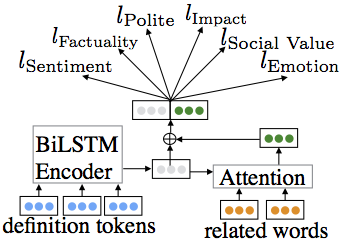
Figure 2: Connotation embedding modeling in §4.1.

4.1.4 Baselines and Models

For each baseline, we implement one classifier per connotation aspect, or, for Emo, one classifier for each emotion. Following Rashkin et al. Rashkin et al. (2016) we implement a Logistic Regression classifier trained on the 300-dimensional pre-trained word embedding for $w$ using the standard L-BFGS optimization algorithm and sample re-weighting (LR). We also implement a majority class baseline (Maj).

We present three variations of our model: (i) trained jointly for all parts of speech and all connotation aspects (CE(J)), (ii) trained on each aspect individually with related word attention (CE+R(S)), and (iii) trained jointly on all parts of speech and all connotation aspects with related word attention (CE+R(J)).

4.2 Connotation Prediction

4.2.1 Data and Parameters

For nouns and adjectives, we train using the aspects described in §3 (6 aspects). For verbs, we train on 9 aspects from Rashkin et al. Rashkin et al. (2016) as well as ‘power’ and ‘agency’ from Sap et al. Sap et al. (2017) (11 aspects total). We split our connotation lexicon (§3) into train (60%), development (20%) and test (20%). For the verb CFs+, we preserve the originally published data splits where possible. We move words only to ensure that all parts of speech for a word are in the same split (e.g., ‘evil’ both as a noun and adj is in the dev set).

We collect dictionary definitions and related words from all seven dictionaries available on the Wordnik API. These are extracted for each word and part-of-speech pair. We preprocess definitions by removing stopwords, punctuation, and the word itself. We use pre-trained Concept-Net numberbatch embeddings Speer et al. (2016).

	Maj	LR	CE+R (S)	CE (J)	CE+R (J)
N/Aj Avg	.304	.594	.589	.597	.597
Verb Avg	.222	.553	.489	.521	.520
All Avg	.251	.568	.524	.548	.547

Table 5: Macro-averaged F1 for connotation prediction on the test set, averaged across aspects. N/Aj indicates noun and adjective.

4.2.2 Results

Label Prediction
We present results on the connotation prediction task to check the quality of our representation learning system. Given dictionary definitions and related words, we predict the labels from our lexicon (§3) and CFs+ (see Table 5).

First, we observe that joint learning (models (J)) improves over training representations individually (CE+R(S)). We hypothesize that joint learning provides regularization across all aspects. Second, we compare joint learning with (CE+R(J)) and without (CE(J) related words to the strong LR baseline. We find that the model with related words (CE+R(J)) is statistically indistinguishable from the baseline (for $p\leq 0.05$). In contrast, our model without related words (CE(J)) is significantly worse than the LR baseline for one aspect (see Appendix D for aspect-level results). Thus we conclude that related words are beneficial for learning connotations.
Overall, our approach provides a single unified feature representation for the lexical connotations of all parts of speech, without any loss in label prediction performance. Specifically, our best representation learning model (CE+R(J)) has comparable label prediction performance to a strong baseline (LR), a baseline that does not learn any kind of representation. We use CE+R(J) to generate connotation embeddings that we use in all further evaluation.

Aspect	Word	Conn Only	Both	Word Only
Social Value	ability (+)	service, imagination, worth, practical	NONE	lack, inability, enough, difficult
Polite	slug (-)	bang, shove, murder, scum	NONE	quote, bug, exception, reference
Impact	merry (+)	glee, exhilaration, pretty, prosperous	cheery, genial, joyful, fun, merriment, jolly joy, delightful, cheerful	amiable, wonderful, crazy, wives

Table 6: Examples of nearest neighbors in the connotation embedding space (Conn Only), the pre-trained word embedding space (Word Only) and all top 50 nearest neighbors in both spaces (Both). NONE indicats no overlap.

Observations
Our connotation representation learning model presents several advantages. Since the model uses dictionary definitions, we can generate representations for slang words (e.g., “gucci” meaning “really good”), where knowledge-base entries (e.g., in Concept-Net) do not capture the slang meaning. For example, in our connotation embedding space, the nearest neighbors of “gucci” include words related to the slang connotations (e.g., “beneficial” – positive impact, not factual), whereas neighbors in a pre-trained word embedding space are specific to the fashion meaning and connotations (e.g., “buy”, “italy”, “textile”). Along with slang, our model can also generate representations for new or rare words (e.g., “merchantile”) that don’t have a pre-trained word representation.

5 Experiments

5.1 Intrinsic Evaluation

To evaluate the connotation embedding space, we look at the $50$ nearest neighbors, by Euclidean distance, of every word in our training and development sets. We find that neighbors in the connotation embedding space are more closely related based on the connotation label than in the pre-trained embedding space.

Looking at example nearest neighbors (Table 6) we see that nearest neighbors in the pre-trained embedding space include antonyms (e.g., “inability” is close to “ability”) and topically related words (e.g., “merry” is close to “wives”), while in the connotation space, neighbors often share connotation labels even though they may be topically or denotatively unrelated. For example, “slug” (noun) is close to many impolite but otherwise unrelated words (e.g., “shove”, “murder”, “scum”) in the connotation embedding space while in the pre-trained space “slug” is close to topically related (e.g., “bug”) but polite words. Therefore, we can see that words with similar connotations are placed closer together than in the pre-trained semantic space.

To quantify the semantic differences, we measure neighbor-cluster connotation label purity. Specifically, for each connotation aspect $a$ (e.g., Social Value) and each non-neutral label $c$ (e.g., valuable (+)), we calculate $r_{c}^{a(C)}$: the average ratio of words with label $c$ to label $-c$ in the set of nearest neighbors of all words with label $c$ for aspect $a$. We compare it against the same ratio for the nearest neighbors selected using the same pre-trained word embeddings as in §4.2, denoted $r_{c}^{a(P)}$.

	$\bm{c}$	Social Val	Polite	Impact
$\bm{r_{c}^{a(C)}}$	+	21.27	2640.14	47.49
	-	5.88	50.00	33.33
$\bm{r_{c}^{a(P)}}$	+	4.70	43.71	4.73
	-	2.38	0.54	8.33

Table 7: Select cluster connotation purity ratios.

We find that across connotation aspects, these ratios are higher for the learned connotation embeddings, compared to pre-trained embeddings. For example, $r_{+}^{\textit{Social Val}(C)}=21.27$ but $r_{+}^{\textit{Social Val}(P)}=4.70$ (see Table 7). This shows the connotation embeddings reshape the pre-trained semantic space.

5.2 Extrinsic Evaluation

We further evaluate our connotation embeddings using the stance detection task, hypothesizing they will lead to improvement. Given a text on a topic (e.g., “gun control”), the task is to predict the stance (pro/con/neutral) towards the topic (see Figure 1).

5.2.1 Methods and Experiments

Models
As a baseline architecture, we implement the bidirectional conditional encoding model Augenstein et al. (2016). This model encodes a text as $h_{T}$ with a BiLSTM, conditioned on a separate topic encoding $h_{P}$, and predicts stance from $h_{T}$ (BiC). We include connotation embeddings through scaled dot-product attention over the noun, adjective, and verb embeddings from the text, with $h_{P}$ as the query (see Figure 3). We experiment with three types of embeddings in the attention: pre-trained word embeddings (BiC+W), our connotation embeddings (BiC+C), and randomly initialized embeddings (BiC+R), as a baseline to measure the importance of attention. We also implement a Bag-of-Word-Vectors baseline (BoWV), encoding the text and topic as separate BoW vectors and passing their concatenation to a Logistic Regression classifier.

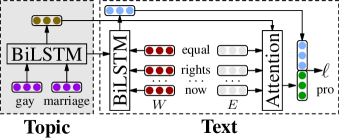
Figure 3: Stance models BiC+$E$; $E\in\{C,W,R\}$.

Data and Parameters
We use the Internet Argument Corpus Abbott et al. (2016): ${\sim}59k$ posts from online debate forums. Of the $16$ total topics, four are large (L, with $>7k$ ex each), five are medium (M, with ${\sim}2k$ ex each), and seven are small (S, with $30$-$300$ ex each).

Since not every text will take a position on every topic, we automatically generate ‘neutral’ examples for the data. To do this, we sample a pro/con example and then assign it a new (different) topic, randomly sampled from the original topic distribution. We split the data into train, development, and test such that no posts by one author are in multiple splits and preprocess the data by removing stopwords and punctuation and lowercasing.

Stance is topic-dependent and as a result, models require numerous training examples for each individual topic. However, many examples are not always available for every topic. Since there are hundreds of thousands of potential topics, the vast majority of which will have very few examples, our goal is to build models that exhibit strong performance across all topics, regardless of size. Therefore, we experiment with three data scenarios: (i) training and evaluating using all the data (All Data), (ii) truncating each topic in training to M size (at most $2k$ examples) and evaluating using all data (Trunc Train), and (iii) truncating each topic to M size in training and in evaluation (Trunc All), so that topics have the same frequency for both training and evaluation.

5.2.2 Results

	All Data	Trunc Train	Trunc All
BoWV	.3587	.3473	.3613
BiC	.5677	.5151	.5244
BiC+R	.5282	.5260	.5128
BiC+W	.5650	.5384	.5421
BiC+C	.5613	.5579∗	.5562∗

Table 8: Stance detection macro-averaged F1 on the test set. ^∗ indicates significance ($p<0.01$) between BiC+C and BiC+W.

We find that when using all of the training data, the pre-trained embeddings and our connotation embeddings perform comparably (significance level $p=0.3$). Note that both the connotation and pre-trained embeddings outperform the random embeddings in all scenarios, showing that the architecture difference is not the only reason for improvement when adding embeddings. We find that in both scenarios where data is limited per topic (Trunc Train and Trunc All), the connotation embeddings improve significantly over the pre-trained word embeddings. In fact, the same trend is visible across varying numbers of training examples (see Figure 4). Our results demonstrate that the connotation information is useful for detecting stance when data is limited.

We find further evidence that the connotation embeddings (BiC+C) make the model robust to loss of training data when we look at the results on the individual topic level. Namely, in setting Trunc Train, BiC+C has a significant improvement (with $p<0.05$) over BiC+W on six topics, including four of the M and truncated L topics. In fact, for the four M/L topics, the average per-topic decrease in F1 for BiC+C is $1/4$ that of BiC+W. These per-topic results further highlight the robustness of BiC+C when training data is restricted.
We conclude that connotation embeddings improve stance performance when training data is limited, suggesting they can be used in future work that generalizes stance models to topics with no training data (i.e. most topics).

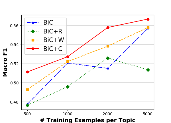
Figure 4: Stance F1 on the test set as number of training examples per topic varies.

6 Conclusion

We create a new lexicon with six new connotation aspects for nouns and adjectives that aligns well with human judgments. We also show that the lexicon confirms hypotheses about semantic divergences between synonyms. We then use our lexicon to train a unified connotation representation for words from all parts of speech, yielding an embedding space that captures more connotative information than pre-trained word embeddings.

We evaluate our connotation representations on stance detection. Since the stance detection tasks encountered in real life concern a very large number of topics, zero-shot and few-shot stance detection are important subtasks. We show that models using our connotation representations are well suited for few-shot stance detection and may also generalize well to zero-shot settings.

In future work, we plan to explore the relationships between connotations, context, and word sense, as well as adapting our methods to learn multi-lingual connotation representations that accurately capture cultural and linguistic variations.

Appendix A Overview

The data and software are provided as supplementary material her: https://github.com/connotationembeddingteam/connotation-embedding.

Aspect	General Inquirer Categories
Social Value	PowGain, PowLoss, PowEnds, PowCon, PowCoop, PowAuPt, PowPt, PowAuth, PowOth, RcEthic, RcRelig, RcGain, RcEnds, RcLoss, Virtue, Vice, WltPt WltTran, WltOth, Food, Object, Doctrin, Academ, Work, NatrObj, Vehicle, Econ@, Goal, EnlPt, EnlOth, EnlLoss, SklPt, SklAsth, SklOth, Exprsv, Legal, COLL, Means MeansLw, Fail, Solve, EndsLw, Try, WlbPhys, WlbGain, WlbPt, WlbLoss, WlbPsyc, Quality, SocRel
Politeness	RspGain, RspLoss, RspOth, AffGain, AffLoss, AffOth, WlbPt, SklPt, EnlPt, Relig, WltPt, Polit, HU, Milit, Legal, Academ, Doctrin
Impact	PosAff, Pleasur, Pain, NegAff, Anomie, NotLw, Vice, Virtue, RcGain, RcLoss, RspLoss, RcEthic, RspOth, WlbPysc, RcEnds, EnlOth, WlbGain, RspGain, EnlGain, EnlEnds, EnlPt, WlbLoss, WlbPt, EnlLoss, SklOth, WlbPhys, Try, Goal, Work
Factuality	$v=\begin{cases}-1&\mbox{if }x\leq-0.25\\ 1&\mbox{if }x\geq 0.25\\ 0&\mbox{otherwise}\\ \end{cases}$ where $x$ is the Imagery score normalized to $[-1,1]$.
Sentiment	$v=\begin{cases}-1&\mbox{if }x\leq-0.25\\ 1&\mbox{if }x\geq 0.25\\ 0&\mbox{otherwise}\\ \end{cases}$ where $x$ is the sentiment score normalized to $[-1,1]$.

Table 9: Categories from the Harvard General Inquirer used in distant labeling connotations.

Appendix B Connotation Labeling

We construct labels for our connotation lexicon (§3) using categories from the following existing resources: HGI – the Harvard General Inquirer (Stone and Hunt, 1963), DAL – the revised Dictionary of Affect in Language (Whissell, 2009), CWN – Connotation WordNet (Kang et al., 2014), and NRCEmoLex – the NRC Emotion Lexicon (Mohammad and Turney, 2013).

The HGI consists of $183$ psycho-sociological categories. Each lexical entry (${\sim}11k$ total) is tagged with a non-zero number of categories. Different senses (noted through brief definitions) and parts-of-speech for the same word have separate entries. The available categories include valence (i.e., positive and negative), words related to a particular entity or social structure (e.g., institutions, communication), and value judgements (e.g., concern with respect).

The DAL consists of ${\sim}8k$ words with scores for 3 categories: pleasantness, activation, and imagery. Word entries include inflection but do not explicitly mark part-of-speech. CWN is a lexicon of connotation polarity scores (ranging from $0$ to $1$) for ${\sim}180k$ words, explicitly marked for part of speech. Finally, NRCEmoLex consists of word entries marked for any number the eight Plutchik emotions (anticipation, joy, trust, fear, surprise, sadness, disgust, anger) as well as positive and negative sentiment. Two versions of the lexicon are available: with and without sense level distinctions. Neither version includes explicit information on part-of-speech, and so we infer part-of-speech using the words provided to distinguish different senses.

We provide the complete distant labeling rules for each of the connotation aspects in Table 9 (see http://www.wjh.harvard.edu/~inquirer/homecat.htm for complete information on abbreviations). Within each connotation aspect, we determine the connotation polarity using the additional categories: Positiv, Negativ, Strong, Weak, Hostile, Submit, Active and Power.

Appendix C Analysis of the Connotation Lexicon

In this section, we provide further analysis of the connotation lexicon as exemplification of its content and properties.

C.1 Human Evaluation

We show the instructions provided to annotators for the manual labeling of samples from the connotation lexicon in §3.3 (see Figures 5 and 6).

We include Cohen’s $kappa$ score for agreement between the lexicon and human annotators for individual connotation aspects in Table 10.

Aspect	Avg Cohen’s $\kappa$
Social Value	0.526
Politeness	0.186
Impact	0.595
Factuality	0.164
Average	0.368

Table 10: Cohen’s $\kappa$ for agreement between the connotation lexicon and human annotators.

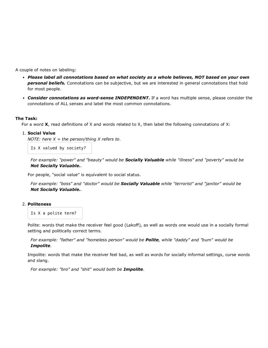
Figure 5: First part of annotator instructions for connotation labeling in §3.3.

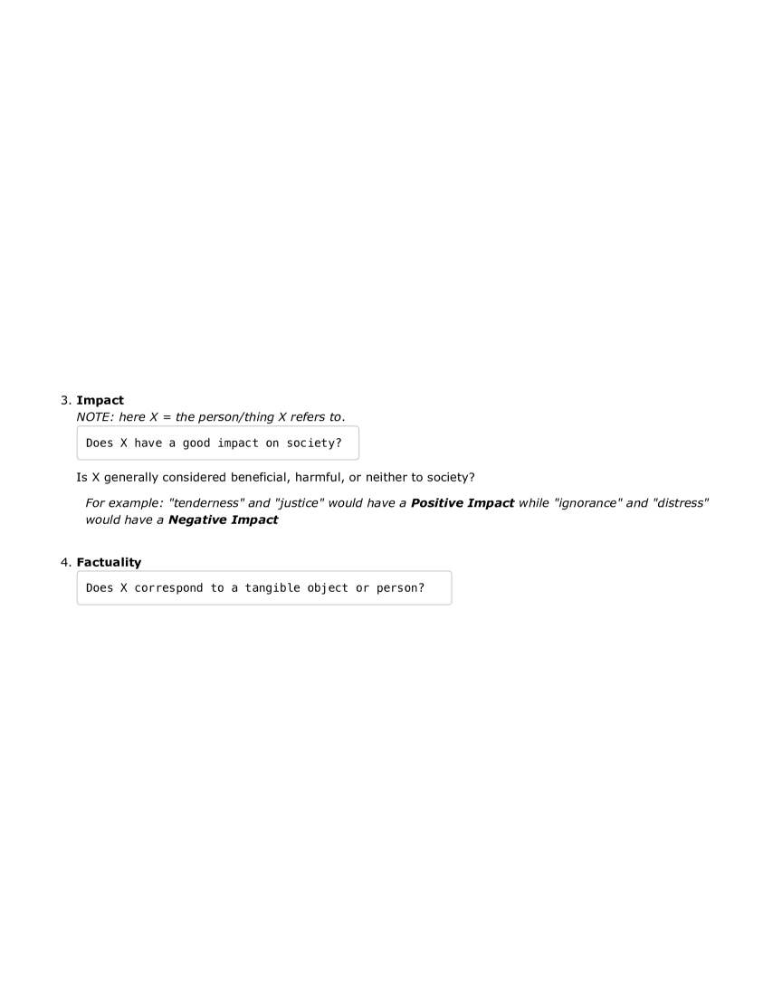
Figure 6: Second part of annotator instructions for connotation labeling in §3.3.

C.2 Gender Bias Analysis

Connotations have been used to study gender bias in movie scripts (Sap et al., 2017) and online media (Field et al., 2019). Here we use our connotation lexicon to analyze gender bias in two new domains: celebrity news (Celebrity) and student reviews of computer science professors (Professors).

We use existing datasets for these domains and the accompanying methodology of Chang and McKeown (2019) to infer word-level gender associations. Then, for the gender-associated words that are in our lexicon, for each connotation aspect and domain, we examine the percentage of positive and negative polarity words and find that these quantify known trends in gender-biased portrayals.

In the Celebrity domain, Factuality highlights the tendency of news media to focus on physical characteristics of female celebrities (Selby, 2014). More words with positive Factuality polarity (tangible concepts and attributes) are associated with women and more words with negative polarity (abstract concepts and attributes) are associated with men. For example, women are described as “beautiful” and “slim”, while men are described as “political” and “presidential”. In fact, even many of the not tangible female-associated words still align with physical attributes (e.g., “chic”), further emphasizing the biased portrayal.

We also find that in the Professors domain, patterns in Social Value and Impact agree with the observations of Chang and McKeown (2019) and with social science literature that finds male teachers are praised more than female teachers for being experts (both socially valuable and positively impacting society). For example, men are associated with positive Social Value (socially valuable) words such as “knowledge” and “experience”, while women are relatively less often associated with the same type of words.

Finally, in the Celebrity domain we find our lexicon reflects the coverage in the media of recent sexual harassment allegations against male celebrities. Namely, women are associated with more positive Social Value words and men are associated with many more negative Social Value words (see Table 11). Overall, our results quantitatively validate previous observations and known patterns of gender bias.

Aspect	Pol	F:M	Examples
Fact	+	54:27	F: beautiful, slim
			M: actor, film
	$-$	26:39	F: style, chic
			M: apology, political
Social Value	+	39:27	F: beauty, body, gold
			M: attempt, evidence
	$-$	3:24	F: blue, dancer, party
			M: abuse, allegation

Table 11: Gender bias examples in the Celebrity news domain. Pol is Polarity (tangible(+) vs. not tangible($-$) and valuable (+) vs. not valuable ($-$)). F:M shows percent of female-associated words to percent of male-associated.

Appendix D Connotation Modeling

D.1 Data

We use dictionary definitions extracted from all available dictionaries on the Wordnik API: American Heritage Dictionary, CMU Pronouncing Dictionary, Macmillan Dictionary, Wiktionary, Webster’s Dictionary, and WordNet. For labels, we use six aspects (see §3): Social Value, Politeness, Impact, Factuality, Sentiment, and Emotional Association. For verbs we use 11 aspects: perspective of the writer on the theme P(wt) and agent P(wa), perspective of the agent on the theme P(at), effect on the theme E(t) and agent E(a), value of the theme V(t) and agent V(a), mental state of the theme S(t) and agent S(a), power, and agency.

D.2 Hyperparameters

All models are trained with hidden size $H=150$, number of definition words $N=42$, number of related words $|R_{w^{t}}|=20$ and dropout of $0.5$ to prevent overfitting. For emotion prediction we set $\theta=0.5$. We use Concept-Net numberbatch embeddings  Speer et al. (2016) because we find empirically that these outperform other pre-trained embeddings (GloVe and dependency-based embeddings Levy and Goldberg (2014)) on the development set.

We tune our only hyperparameters on the development set: the weights $\lambda_{a}$ for the contribution of each loss term $\mathcal{L}^{a}$ to the total loss $\sum_{a}\lambda_{a}\mathcal{L}^{a}$ (see 4.1.3). We experiment with $10$ manually selected weight combinations, where each $\lambda_{a}\in(0,5)$. We find that the optimal weights are:

• $\lambda_{a}=0.3$ for $a\in\{SocialVal,Impact$, $V(t),V(a),power,agency\}$

• $\lambda_{a}=0.167$ for $a\in\{Fact,Sent\}$

• $\lambda_{a}=1.0$ for $a\in\{P(wt),P(wa),P(at)$, $E(t)$, $E(a)$, $S(t),S(a)\}$

• $\lambda_{a}=0.5$ for $a=Polite$

• $\lambda_{a}=3.0$ for $a=Emo$

Additionally, we compute expected validation performance (Dodge et al., 2019) on each connotation aspect individually (see Table 12).

	Best Dev	$\mathbb{E}[$Dev$]$
Social Val	0.681	0.700
Polite	0.540	0.554
Impact	0.704	0.711
Fact	0.546	0.565
Sent	0.612	0.631
Emo	0.574	0.584
Avg	0.610	0.610
P(wt)	0.525	0.583
P(wa)	0.580	0.577
P(at)	0.606	0.613
E(t)	0.668	0.686
E(a)	0.596	0.618
V(t)	0.376	0.469
V(a)	0.463	0.459
S(t)	0.600	0.642
S(a)	0.611	0.603
power	0.466	0.493
agency	0.426	0.487
Avg	0.538	0.542
Avg	0.563	0.563

Table 12: Best macro-averaged F1 on the development set and expected validation score Dodge et al. (2019) for our connotation representation learning model on all connotation aspects.

D.3 Training

We optimize using Adam Kingma and Ba (2014) with learning rate $0.001$ and minibatch-size of $64$ for $80$ epochs with early stopping. We optimize the parameters $W^{a}$, $b^{a}$ for each noun and adjective aspect $a$ separately from the parameters for each verb aspect $a$, allowing both to update the parameters of the definition encoder, and attention layer.

D.4 Detailed results

We present aspect-level results for the task of connotation label prediction (see Table13).

	Maj	LR	CE+R (S)	CE (J)	CE+R (J)
Social Val	.228	.664	.651	.632	.651
Polite	.311	.470	.467	.518	.464
Impact	.278	.669	.681	.687	.704
Fact	.271	.576	.531	.549	.560
Sent	.247	.585	.606	.615	.615
Emo	.487	.604	.599	.578	.587
Avg	.304	.594	.589	.597	.597
P(wt)	.246	.501	.437	.481	.439
P(wa)	.213	.564	.487	.544	.583
P(at)	.204	.649	.553	.623	.629
E(t)	.156	.721	.673	.655	.661
E(a)	.226	.573	.420	.557	.530
V(t)	.109	.369	.365	.391	.373
V(a)	.320	.449	.428	.375	.370
S(t)	.286	.640	.548	.586	.629
S(a)	.203	.551	.481	.543	.537
power	.294	.476	.467	.474	.480
agency	.182	.589	.515	.505	.490
Avg	.222	.553	.489	.521	.520
Avg	.251	.568	.524	.548	.547

Table 13: Macro-averaged F1 results for connotation prediction on the test set. The upper part shows noun/adjective aspect results, the bottom shows verb aspect results. Underline indicates the best performing model per row. Bold indicates the best performing joint learning model per row.

Appendix E Extrinsic Stance Evaluation

Topic	# Ex	# C	# P	# N
abortion	12453	3962	5236	3255
gay marriage	11037	2907	5082	3048
gun control	10119	4610	2681	2828
evolution	9896	2586	4480	2830
existence of God	7227	2588	2517	2122
death penalty	2834	995	951	888
humans are responsible	1608	560	538	510
marijuana legalization	1491	328	697	466
communism is better than capitalism	1279	618	277	384
illegal immigration	291	108	87	96
health care reform	201	76	51	74
legalize prostitution	199	57	88	54
Israel	100	29	38	33
vegetarian diet is best	79	29	29	21
women in combat	47	15	19	13
minimum wage	27	9	8	10
Overall	58888	19477	22779	16632

Table 14: Statistics for the stance detection dataset. C indicates ‘con’, P indicates ‘pro’, N indicates ’neutral’.

E.1 Dataset Details

We map the topic-stance annotations in the Internet Argument Corpus to individual topics and labels (e.g., ‘pro-life’ $\rightarrow$ topic ‘abortion’ with label ‘con’). We show dataset statistics in Table 14, where topics in the upper part are large sized, topics in the middle part are medium sized, and topics in the lower part are small sized.

E.2 Training Details

We split the data $60\%$ train, $20\%$ development, and $20\%$ test. We train our models using pre-trained 100-dimensional word embeddings from GloVe Pennington et al. (2014), as these are comparable to and more time-efficient than larger word embeddings. We use a hidden size of $60$, dropout of $0.5$, and train for $70$ epochs with early stopping on the development set. We optimize Adam with learning rate $0.001$ and minibatch-size of $64$ on the cross-entropy loss. Our hyperparameters are set following Augenstein et al. (2016).

When truncating to medium size in §5.2, we truncate train topics to at most $2000$ examples (Trunc Train and Trunc All) and development and test topics to at most $600$ examples (Trunc All).

E.3 Topic Stance Analysis

We present a detailed analysis of the results of the models BiC+W and BiC+C on the stance detection on individual topics. First, we find that when the models are trained with all of the data (All Data), there are statistically significant differences on only two topics, one of which is very small (see Table 15(a)). This is further evidence that the models are comparable in this setting.

We then find that when trained with truncated training data (see §5.2 for details) (Trunc Train), BiC+C improves over BiC+W on six topics, including four of the medium or truncated large topics (see Table 15(b)). When trained and evaluated with truncated data (Trunc All), BiC+W and BiC+C have statistically significant improvements over each other on the same number of topics (two each) but BiC+C is significantly better overall (see Table 15(c)). These results further show that connotations help to learn stance when data is limited.

Topic	BiC +W	BiC +C
abortion	.49	.49
gay marriage	.47	.48
gun control	.53	.55
evolution	.43	.44
existence of God	.52	.52
death penalty	.45	.50†
humans are responsible	.49	.54
marijuana legalization	.51	.50
communism is better than capitalism	.52	.54
illegal immigration	.34	.38
health care reform	.64	.91
legalize prostitution	.40	.53
Israel	.66	.42
vegetarian diet is best	.52†	.33
women in combat	.28	.30
minimum wage	.30	.22
Overall	.57	.57

(a) On All Data.

Topic	BiC +W	BiC +C
abortion	.46	.47
gay marriage	.48	.46
gun control	.50	.55∗
evolution	.41	.43∗†
existence of God	.48	.51∗
death penalty	.48	.50
humans are responsible	.45	.53∗†
marijuana legalization	.51	.50
communism is better than capitalism	.53	.54
illegal immigration	.45∗	.36
health care reform	.62	.64∗†
legalize prostitution	.49	.50
Israel	.54	.44
vegetarian diet is best	.10	.11∗
women in combat	.52	.36
minimum wage	.22	.33
Overall	.54	.56∗†

(b) On Trunc Train.

Topic	BiC +W	BiC +C
abortion	.49	.48
gay marriage	.49∗	.46
gun control	.51	.50
evolution	.43	.43
existence of God	.49	.47
death penalty	.48	.46
humans are responsible	.46	.55∗†
marijuana legalization	.50	.49
communism is better than capitalism	.55	.52
illegal immigration	.44	.44
health care textit reform	.54	.64∗†
legalize prostitution	.47	.51
Israel	.41	.56
vegetarian diet is best	.52∗†	.50
women in combat	.43	.47
minimum wage	.33	.35
Overall	.54	.56∗†

(c) On Trunc All.

Table 15: Macro F1 results on the test set for three different data scenarios. ^∗ indicates significance with $p<0.05$, ^† indicates significane with $p<0.01$.

References

- Abbott et al. (2016) Rob Abbott, Brian Ecker, Pranav Anand, and Marilyn A. Walker. 2016. Internet argument corpus 2.0: An sql schema for dialogic social media and the corpora to go with it. In Proceedings of the Tenth International Conference on Language Resources and Evaluation.
- Asur and Huberman (2010) Sitaram Asur and Bernardo A. Huberman. 2010. Predicting the future with social media. In Web Intelligence.
- Aubakirova and Bansal (2016) Malika Aubakirova and Mohit Bansal. 2016. Interpreting neural networks to improve politeness comprehension. In Proceedings of the 2016 Conference on Empirical Methods in Natural Language Processing, pages 2035–2041, Austin, Texas. Association for Computational Linguistics.
- Augenstein et al. (2016) Isabelle Augenstein, Tim Rocktäschel, Andreas Vlachos, and Kalina Bontcheva. 2016. Stance detection with bidirectional conditional encoding. In Proceedings of the 2016 Conference on Empirical Methods in Natural Language Processing.
- Bhagat and Hovy (2013) Rahul Bhagat and Eduard H. Hovy. 2013. What is a paraphrase? Computational Linguistics, 39:463–472.
- Brown and Levinson (1987) Penelope Brown and Stephen C. Levinson. 1987. Politeness: Some universals in language usage. Cambridge University Press.
- Carpuat (2015) Marine Carpuat. 2015. Connotation in translation. In Proceedings of 6th Workshop on Computational Approches to Subjectivity, Sentiment and Social Media Analysis.
- Chang and McKeown (2019) Serina Chang and Kathleen McKeown. 2019. Automatically inferring gender associations from language. In Proceedings of 9th International Joint Conference on Natural Language Processing.
- Choi and Wiebe (2014) Yoonjung Choi and Janyce Wiebe. 2014. +/-effectwordnet: Sense-level lexicon acquisition for opinion inference. In Proceedings of the 2014 Conference on Empirical Methods in Natural Language Processing.
- Clark (1992) E. V. Clark. 1992. Conventionality and contrasts: Pragmatic principles with lexical consequences. In Frame, Fields,and Contrasts: New Essays in Semantic Lexical Organization, pages 171–188. Lawrence Erlbaum Associates, Hillsdale, NJ.
- Cohen (1988) Robin Cohen. 1988. On the relationship between user models and discourse models. Computational Linguistics, 14(3).
- Colston and Katz (2005) Herbert L. Colston and Albert N. Katz, editors. 2005. Figurative Language Comprehension: Social and Culturla Influences. Lawrence Erlbaum Associates, Inc.
- Conforti et al. (2018) Costanza Conforti, Mohammad Taher Pilehvar, and Nigel Collier. 2018. Towards automatic fake news detection: Cross-level stance detection in news articles. In Proceedings of the First Workshop on Fact Extraction and VERification (FEVER).
- Danescu-Niculescu-Mizil et al. (2013) Cristian Danescu-Niculescu-Mizil, Moritz Sudhof, Dan Jurafsky, Jure Leskovec, and Christopher Potts. 2013. A computational approach to politeness with application to social factors. In Proceedings of the 51st Annual Meeting of the Association for Computational Linguistics (Volume 1: Long Papers), pages 250–259, Sofia, Bulgaria. Association for Computational Linguistics.
- Dodge et al. (2019) Jesse Dodge, Suchin Gururangan, Dallas Card, Roy Schwartz, and Noah A. Smith. 2019. Show your work: Improved reporting of experimental results. In EMNLP/IJCNLP.
- Faulkner (2014) Adam Faulkner. 2014. Automated classification of stance in student essays: An approach using stance target information and the wikipedia link-based measure. In Proceedings of the Twenty-Seventh International Florida Artificial Intelligence Research Society Conference.
- Feng et al. (2011) Song Feng, Ritwik Bose, and Yejin Choi. 2011. Learning general connotation of words using graph-based algorithms. In Proceedings of the 2011 Conference on Empirical Methods in Natural Language Processing.
- Feng et al. (2013) Song Feng, Jun Seok Kang, Polina Kuznetsova, and Yejin Choi. 2013. Connotation lexicon: A dash of sentiment beneath the surface meaning. In Proceedings of the 51st Annual Meeting of the Association for Computational Linguistics (Volume 1: Long Papers), pages 1774–1784, Sofia, Bulgaria. Association for Computational Linguistics.
- Field et al. (2019) Anjalie Field, Gayatri Bhat, and Yulia Tsvetkov. 2019. Contextual affective analysis: A case study of people portrayals in online #metoo stories. Proceeding of the 13th Internaltional AAAI Conference on Web and Social Media.
- Ghanem et al. (2018) Bilal Ghanem, Paolo Rosso, and Francisco Rangel. 2018. Stance detection in fake news a combined feature representation. In Proceedings of the First Workshop on Fact Extraction and VERification (FEVER).
- Guralnik (1958) David B. Guralnik. 1958. Connotation in dictionary definition. College Compoistion and Communication, 9:90–93.
- Hanselowski et al. (2018) Andreas Hanselowski, Avinesh PVS, Benjamin Schiller, Felix Caspelherr, Debanjan Chaudhuri, Christian M. Meyer, and Iryna Gurevych. 2018. A retrospective analysis of the fake news challenge stance-detection task. In Proceedings of the 27th International Conference on Computational Linguistics, pages 1859–1874, Santa Fe, New Mexico, USA. Association for Computational Linguistics.
- Hartmann et al. (2019) Mareike Hartmann, Tallulah Jansen, Isabelle Augenstein, and Anders Søgaard. 2019. Issue framing in online discussion fora. In Proceedings of 2019 Annual Conference of the North American Chapter of the Association for Computational Linguistics: Human Language Technologies.
- Hasan and Ng (2013) Kazi Saidul Hasan and Vincent Ng. 2013. Stance classification of ideological debates: Data, models, features, and constraints. In Proceedings of the Sixth International Joint Conference on Natural Language Processing, pages 1348–1356, Nagoya, Japan. Asian Federation of Natural Language Processing.
- Hasan and Ng (2014) Kazi Saidul Hasan and Vincent Ng. 2014. Why are you taking this stance? identifying and classifying reasons in ideological debates. In Proceedings of the 2014 Conference on Empirical Methods in Natural Language Processing.
- Hoyle et al. (2019) Alexander Hoyle, Lawrence Wolf-Sonkin, Hanna M. Wallach, Ryan Cotterell, and Isabelle Augenstein. 2019. Combining sentiment lexica with a multi-view variational autoencoder. In Proceedings of 2019 Annual Conference of the North American Chapter of the Association for Computational Linguistics: Human Language Technologies.
- Kang et al. (2014) Jun Seok Kang, Song Feng, Leman Akoglu, and Yejin Choi. 2014. ConnotationWordNet: Learning connotation over the Word+Sense network. In Proceedings of the 52nd Annual Meeting of the Association for Computational Linguistics (Volume 1: Long Papers), pages 1544–1554, Baltimore, Maryland. Association for Computational Linguistics.
- Kingma and Ba (2014) Diederik Kingma and Jimmy Ba. 2014. Adam: A method for stochastic optimization. In Proceedings of the 2nd International Conference on Representation Learning.
- Klenner (2017) Manfred Klenner. 2017. An object-oriented model of role framing and attitude prediction. In Proceedings of the 12th International Conference on Computational Semantics.
- Klenner and Clematide (2016) Manfred Klenner and Simon Clematide. 2016. How factuality determines sentiment inferences. In Proceedings of the Fifth Joint Conference on Lexical and Computational Semantics (*SEM@ACL.
- Klenner et al. (2018) Manfred Klenner, Josef Ruppenhofer, Michael Wiegand, and Melanie Siegel. 2018. Offensive language without offensive words (olwow). In Proceedings of KOVENS.
- Klenner et al. (2017) Manfred Klenner, Don Tuggener, and Simon Clematide. 2017. Stance detection in Facebook posts of a German right-wing party. In Proceedings of the 2nd Workshop on Linking Models of Lexical, Sentential and Discourse-level Semantics, pages 31–40, Valencia, Spain. Association for Computational Linguistics.
- Lakoff (1973) Robin Lakoff. 1973. The logic of politeness; or minding your p’s and q’s. In 9th Regional Meeting of the Chicago Linguistic Society, Chicago.
- Levy and Goldberg (2014) Omer Levy and Yoav Goldberg. 2014. Dependency-based word embeddings. In Proceedings of the 52nd Annual Meeting of the Association for Computational Linguistics (Volume 2: Short Papers), pages 302–308, Baltimore, Maryland. Association for Computational Linguistics.
- Li et al. (2018) Chang Li, Aldo Porco, and Dan Goldwasser. 2018. Structured representation learning for online debate stance prediction. In Proceedings of the 27th International Conference on Computational Linguistics, pages 3728–3739, Santa Fe, New Mexico, USA. Association for Computational Linguistics.
- Mohammad (2012) Saif Mohammad. 2012. #emotional tweets. In *SEM 2012: The First Joint Conference on Lexical and Computational Semantics – Volume 1: Proceedings of the main conference and the shared task, and Volume 2: Proceedings of the Sixth International Workshop on Semantic Evaluation (SemEval 2012), pages 246–255, Montréal, Canada. Association for Computational Linguistics.
- Mohammad et al. (2013a) Saif Mohammad, Svetlana Kiritchenko, and Xiaodan Zhu. 2013a. NRC-canada: Building the state-of-the-art in sentiment analysis of tweets. In Second Joint Conference on Lexical and Computational Semantics (*SEM), Volume 2: Proceedings of the Seventh International Workshop on Semantic Evaluation (SemEval 2013), pages 321–327, Atlanta, Georgia, USA. Association for Computational Linguistics.
- Mohammad et al. (2013b) Saif Mohammad, Svetlana Kiritchenko, and Xiaodan Zhu. 2013b. Nrc-canada: Building the state-of-the-art in sentiment analysis of tweets. In Proceedings of the seventh international workshop on Semantic Evaluation Exercises (SemEval-2013), Atlanta, Georgia, USA.
- Mohammad (2018a) Saif M. Mohammad. 2018a. Obtaining reliable human ratings of valence, arousal, and dominance for 20,000 english words. In Proceedings of The Annual Conference of the Association for Computational Linguistics, Melbourne, Australia.
- Mohammad (2018b) Saif M. Mohammad. 2018b. Word affect intensities. In Proceedings of the 11th Edition of the Language Resources and Evaluation Conference, Miyazaki, Japan.
- Mohammad et al. (2016) Saif M. Mohammad, Svetlana Kiritchenko, Parinaz Sobhani, Xiao-Dan Zhu, and Colin Cherry. 2016. Semeval-2016 task 6: Detecting stance in tweets. In Proceedings of the 10th International Workshop on Semantic Evaluation.
- Mohammad and Turney (2010) Saif M. Mohammad and Peter D. Turney. 2010. Emotions evoked by common words and phrases: Using mechanical turk to create an emotion lexicon. In Proceedings of 2010 Annual Conference of the North American Chapter of the Association for Computational Linguistics: Human Language Technologies.
- Mohammad and Turney (2013) Saif M. Mohammad and Peter D. Turney. 2013. Crowdsourcing a word-emotion association lexicon. Computational Intelligence, 29(3):436–465.
- Murakami and Putra (2010) Akiko Murakami and Raymond H. Putra. 2010. Support or oppose? classifying positions in online debates from reply activities and opinion expressions. In Proceedings of the 23rd International Conference on Computational Linguistics.
- Pavlick et al. (2015) Ellie Pavlick, Pushpendre Rastogi, Juri Ganitkevitch, Benjamin Van Durme, and Chris Callison-Burch. 2015. PPDB 2.0: Better paraphrase ranking, fine-grained entailment relations, word embeddings, and style classification. In Proceedings of the 53rd Annual Meeting of the Association for Computational Linguistics and the 7th International Joint Conference on Natural Language Processing (Volume 2: Short Papers), pages 425–430, Beijing, China. Association for Computational Linguistics.
- Pennington et al. (2014) Jeffrey Pennington, Richard Socher, and Christopher D. Manning. 2014. Glove: Global vectors for word representation. In Proceedings of the 2014 Conference on Empirical Methods in Natural Language Processing.
- Plutchik (2001) Robert Plutchik. 2001. The nature of emotions: Human emotions have deep evolutionary roots, a fact that may explain their complexity and provide tools for clinical practice. American Scientist, 89(4):344–350.
- Potthast et al. (2018) Martin Potthast, Johannes Kiesel, Kevin Reinartz, Janek Bevendorff, and Benno Stein. 2018. A stylometric inquiry into hyperpartisan and fake news. Proceedings of the 56th Annual Meeting of the Association for Computational Linguistics (Volume 1: Long Papers).
- Rashkin et al. (2017) Hannah Rashkin, Eric Bell, Yejin Choi, and Svitlana Volkova. 2017. Multilingual connotation frames: A case study on social media for targeted sentiment analysis and forecast. In Proceedings of the 55th Annual Meeting of the Association for Computational Linguistics (Volume 2: Short Papers), pages 459–464, Vancouver, Canada. Association for Computational Linguistics.
- Rashkin et al. (2016) Hannah Rashkin, Sameer Singh, and Yejin Choi. 2016. Connotation frames: A data-driven investigation. In Proceedings of the 54th Annual Meeting of the Association for Computational Linguistics (Volume 1: Long Papers), pages 311–321, Berlin, Germany. Association for Computational Linguistics.
- Riedel et al. (2017) Benjamin Riedel, Isabelle Augenstein, Georgios P. Spithourakis, and Sebastian Riedel. 2017. A simple but tough-to-beat baseline for the fake news challenge stance detection task. ArXiv, abs/1707.03264.
- Rubin (2006) David C. Rubin. 2006. The basic-systems model of episodic memory. Perspectives on psychological science : a journal of the Association for Psychological Science, 1 4:277–311.
- Sap et al. (2017) Maarten Sap, Marcella Cindy Prasettio, Ari Holtzman, Hannah Rashkin, and Yejin Choi. 2017. Connotation frames of power and agency in modern films. In Proceedings of the 2017 Conference on Empirical Methods in Natural Language Processing.
- Saurí and Pustejovsky (2009) Roser Saurí and James Pustejovsky. 2009. Factbank: a corpus annotated with event factuality. Language Resources and Evaluation, 43:227–268.
- Selby (2014) Jenn Selby. 2014. Cate blanchett calls out red carpet sexism: “do you do this to the guys?”. In Independent.
- Somasundaran and Wiebe (2010) Swapna Somasundaran and Janyce Wiebe. 2010. Recognizing stances in ideological on-line debates. In Proceedings of 2010 Annual Conference of the North American Chapter of the Association for Computational Linguistics: Human Language Technologies.
- Speer et al. (2016) Robyn Speer, Joshua Chin, and Catherine Havasi. 2016. Conceptnet 5.5: An open multilingual graph of general knowledge. In Proceedings of the Thirtieth Association for the Advancement of Artificial Intelligence Conference on Artificial Intelligence.
- Sridhar et al. (2015) Dhanya Sridhar, James Foulds, Bert Huang, Lise Getoor, and Marilyn Walker. 2015. Joint models of disagreement and stance in online debate. In Proceedings of the 53rd Annual Meeting of the Association for Computational Linguistics and the 7th International Joint Conference on Natural Language Processing (Volume 1: Long Papers), pages 116–125, Beijing, China. Association for Computational Linguistics.
- Stone and Hunt (1963) Philip J. Stone and E. B. Hunt. 1963. A computer approach to content analysis: studies using the general inquirer system. In AFIPS ’63 (Spring).
- Tausczik and Pennebaker (2009) Yla R. Tausczik and James W. Pennebaker. 2009. The psychological meaning of words: Liwc and computerized text analysis methods. In Journal of Language and Social Psychology.
- Vaswani et al. (2017) Ashish Vaswani, Noam Shazeer, Niki Parmar, Jakob Uszkoreit, Llion Jones, Aidan N. Gomez, Lukasz Kaiser, and Illia Polosukhin. 2017. Attention is all you need. In Proceedings of the Thirty-First Annual Conference on Neural Information Systems.
- Webson et al. (2020) Albert Webson, Zhizhong Chen, Carsten Eickhoff, and Ellie Pavlick. 2020. Are “undocumented workers” the same as “illegal aliens”? disentangling denotation and connotation in vector spaces. In Proceedings of the 2020 Conference on Empirical Methods in Natural Language Processing.
- Whissell (1989) Cynthia Whissell. 1989. The dictionary of affect in language. In The Measurement of Emotions, pages 113–131.
- Whissell (2009) Cynthia Whissell. 2009. Using the revised dictionary of affect in language to quantify the emotional undertones of samples of natural language. Psychological reports, 105 2:509–21.
- Xu et al. (2018) Chang Xu, Cécile Paris, Surya Nepal, and Ross Sparks. 2018. Cross-target stance classification with self-attention networks. In Proceedings of The Annual Conference of the Association for Computational Linguistics.