Modeling Personalized Item Frequency Information for Next-basket Recommendation

Abstract.

Next-basket recommendation (NBR) is prevalent in e-commerce and retail industry. In this scenario, a user purchases a set of items (a basket) at a time. NBR performs sequential modeling and recommendation based on a sequence of baskets. NBR is in general more complex than the widely studied sequential (session-based) recommendation which recommends the next item based on a sequence of items. Recurrent neural network (RNN) has proved to be very effective for sequential modeling, and thus been adapted for NBR. However, we argue that existing RNNs cannot directly capture item frequency information in the recommendation scenario.

Through careful analysis of real-world datasets, we find that personalized item frequency (PIF) information (which records the number of times that each item is purchased by a user) provides two critical signals for NBR. But, this has been largely ignored by existing methods. Even though existing methods such as RNN based methods have strong representation ability, our empirical results show that they fail to learn and capture PIF. As a result, existing methods cannot fully exploit the critical signals contained in PIF. Given this inherent limitation of RNNs, we propose a simple item frequency based k-nearest neighbors (kNN) method to directly utilize these critical signals. We evaluate our method on four public real-world datasets. Despite its relative simplicity, our method frequently outperforms the state-of-the-art NBR methods – including deep learning based methods using RNNs – when patterns associated with PIF play an important role in the data.

1. Introduction

Recommendation systems have been applied in many different applications (Aggarwal et al., 2016). NBR is a type of recommendation problem that aims to recommend a set of items to a user based on his/her historical purchased baskets (Rendle et al., 2010)(Ying et al., 2018)(Wang et al., 2015)(Yu et al., 2016), which is prevalent in E-commerce and retail industry. Unlike top-$n$ recommendation (whose historical record is a set of items) (Ning et al., 2015) and sequential recommendation (whose historical record is a sequence of items) (Ludewig et al., 2019), the historical record of the next-basket recommendation is a sequence of sets or sequential sets (whose element is a set). Considering the historical records, top-$n$ recommendation and sequential/session-based recommendation can be seen as special cases of NBR when the NBR only has one basket and has a sequence of baskets whose size are all of 1, respectively. But in recommendation step, top-$n$ recommendation only recommends new items that are not contained in the user’s historical records, whereas both sequential/session-based recommendation and NBR recommend new and old items. Even though sequential/session-based recommendation is similar to NBR, we cannot directly apply sequential/session-based recommendation method to do NBR without messing up the information existing in the sequential sets.

The challenging part in NBR is how to model the relation between the historical records and recommended items. Existing NBR methods use different ways to model the information in the historical records as the user profile and capture user-item interactions for predicting the next basket. RNNs have become one of the mainstream choices as it is easy to be tweaked for sequential modeling. However, we argue that existing RNNs cannot directly capture item frequency information in the recommendation scenario.

Recently, repeated behaviors are found to bring considerable performance improvement in both sequential/session-based recommendation (Wang et al., 2019b)(Ren et al., 2019) and NBR (Hu and He, 2019). It is based on the observation that repeated purchases widely exist in the users’ records. However, our analysis shows that PIF contains more information than repeated purchase pattern. We observe that similar users’ PIF also contains collaborative purchase pattern. This new pattern shows that if a user repeatedly purchases a item, similar users are likely to purchase the same item. Existing methods fail to fully utilize this useful information contained in PIF.

In this paper, we propose a simple k-nearest neighbors (kNN) based method which directly captures the two useful patterns associated with PIF. To demonstrate the effectiveness, we also observe and analyze the limitation of existing methods to capture the important patterns associated with PIF as they cannot learn the vector addition well. In summary, our contributions are as follows:

• We analyze two patterns associated with PIF and the target basket. The collaborative purchase pattern that PIF can contribute to the NBR in a collaborative way is discovered.

• We discover the difficulty of RNNs in learning vector addition in recommendation setting. To our best knowledge, we are the first to present and analyze this phenomenon.

• We propose a simple and effective kNN based method to directly capture the two useful patterns associated with PIF. The temporal dynamics is also considered in the proposed method.

• We perform experiments on four real-world data sets to demonstrate the effectiveness of the proposed method.

The rest of the paper is organized as follows: Section 2 presents the preliminaries. In section 3, we describe our proposed method. In section 4, we discuss the related work. In section 5, we evaluate our method. Section 6 provides some concluding remarks and future directions.

2. PRELIMINARIES

In this section, the NBR problem is first formally defined. Next, we analyze the patterns associated with PIF for NBR. Our analysis towards real-world data sets reveals that PIF contains two important signals for the next target basket. Finally, we summarize the existing methods, and discuss the their difficulty in learning PIF.

2.1. Problem Definition

Given the historical purchase records of a user $\small\{\mathbf{v}_{1},\mathbf{v}_{2},...,\mathbf{v}_{i},...,\mathbf{v}_{t}\}$, where a set of items (a basket) at the $i$-th time step is represented as a 0/1 vector $\small\mathbf{v}_{i}$ whose entry $c_{j}$ ($j\in[0,d]$) is set to 1 if the corresponding item appears in the basket, our goal is to predict the next set of items (next basket) $\small\mathbf{\hat{v}_{t+1}}$.

Following the literature (Rendle et al., 2010)(Yu et al., 2016), we consider a fixed-size set with $s$ items as the recommendation for the next basket.

2.2. Relation between PIF and Target Basket

In this section, we discuss two important patterns associated with PIF that can help predict the target next basket: repeated purchase pattern and collaborative purchase pattern.

Repeated purchase behavior in grocery shopping and online activities has been studied in the areas of economics and psychology theoretically and empirically (Anderson et al., 2014)(Benson et al., 2016)(Dawes et al., 2015)(Jacoby and Kyner, 1973). This pattern has been used in recent sequential/session-based recommendation method (Ren et al., 2019)(Wang et al., 2019b) and NBR method (Hu and He, 2019)(Wan et al., 2018), and is shown to get considerable performance gain. Specifically, a simple baseline which recommends the user-specific most frequent items can sometimes outperform many existing methods (Hu and He, 2019). The good performance of this baseline comes from the assumption that the next target basket often contains items that have appeared in the user’s historical records. And the higher PIF is associated with a higher probability of the corresponding item to appear in the target basket again. However, this assumption has a limitation that the PIF only helps the target user. It ignores the collaboration among different users. This is the core idea of collaborative filter (Konstan et al., 1997). A natural question is whether PIF can help in a collaborative manner. To verify this, we investigate the co-occurrence of the same item to simultaneously appear in the past baskets of the similar users and the next basket of the target user on four real-world data sets (the details of the data are in section 5.1.1). To compare with repeated purchase pattern, we also investigate the co-occurrence of the same item to simultaneously appear in the past baskets of the target user and the next basket of the target user. We simply use the PIF vector ($\small PIF_{vector}=\sum_{i=1}^{t}\mathbf{v}_{i}$) to represent each user. For each user, his/her top 300 nearest neighbors (the total number of users in all data sets is no less than 10,000) are found based on the PIF vector. Denote the set of all items in target user’s past baskets as $P$. Denote the set of all items in the neighbors’ past baskets as set $N$. The target basket is denoted as $T$. We calculate the following four ratios:

• $Recall_{P}$: The average recall of using $P$ to retrieve items in $T$. Formally, $\small Recall_{P}=\frac{|P\cap T|}{|T|}$. It represents the ratio of items captured by repeated purchase pattern.

• $Recall_{N}$: The average recall of using $N$ to retrieve items in $T$. Formally, $\small Recall_{N}=\frac{|N\cap T|}{|T|}$. It represents the ratio of items captured by collaborative purchase pattern.

• $Recall_{P\cap N}$: The average recall of using $P\cap N$ to retrieve items in $T$. Formally, $\small Recall_{N}=\frac{|P\cap N\cap T|}{|T|}$. It represents the ratio of items captured by both repeated purchase pattern and collaborative purchase pattern.

• $Recall_{\overline{P}\cap\overline{N}}$: The average recall of using $\overline{P}\cap\overline{N}$ to retrieve items in $T$. Formally, $\small Recall_{\overline{P}\cap\overline{N}}=\frac{|\overline{P}\cap\overline{N}\cap T|}{|T|}$. It represents the ratio of items not captured by repeated purchase pattern and collaborative purchase pattern.

Table 1. The importance of two patterns.

Data	$Recall_{P}$	$Recall_{N}$	$Recall_{P\cap N}$	$Recall_{\overline{P}\cap\overline{N}}$
ValuedShopper	0.6570	0.9808	0.6490	0.0111
Instacart	0.5711	0.8338	0.5056	0.1007
Dunnhumby	0.2777	0.5580	0.2432	0.4075
TaFeng	0.1378	0.8614	0.1256	0.1262

From Table  1, we can make several observations. First, $Recall_{P}$ indicates that the repeated purchase pattern plays a considerable role in four data sets but varies dramatically across different data sets. Second, $Recall_{N}$ indicates that the collaborative purchase pattern plays much more important role in all four data sets. It can help retrieve more than half items in the target basket. Surprisedly, this ratio can increase to more than 0.8 in three data sets. Note that, here we only use 300 nearest neighbors. It is expected that $Recall_{N}$ will increase if we increase the number of neighbors. Third, $Recall_{P\cap N}$ indicates that these two patterns have overlap. Based on $Recall_{N}-Recall_{P\cap N}$, we can also infer that the collaborative purchase pattern provides extra signal related to the target basket. Fourth, $Recall_{\overline{P}\cap\overline{N}}$ indicates that only a small part of items are not covered by the two patterns. It implies that the unseen patterns are only a small part in the next basket. Based on $1-Recall_{\overline{P}\cap\overline{N}}$, we find that combining both patterns can achieve better performance than any single pattern. Note that above analysis is based on complete $P$ and $N$ whose size is still large. In general, we only recommend a small number of items in NBR. Nonetheless this analysis demonstrates the potential incorporating PIF in NBR.

2.3. Existing NBR Methods

MC based methods: Rendle et al. (Rendle et al., 2010) propose the classical NBR method which is based on factorization and Markov chain. Their method models the personalized item-item transition matrix between any pair of consecutive baskets. Wang et al. (Wang et al., 2015) propose a similar Markov chain model. Instead of using tensor factorization, they propose to use pooling to aggregate the items in the recent basket as the recent basket representation and predict the next basket based on the aggregated representation. Ying et al. (Ying et al., 2018) enhance the structure in (Wang et al., 2015) and use attention mechanism to replace the pooling operation. The attention mechanism can focus on the most relevant items, which brings performance improvement. Also, they partition historical items into two sets. The items in the recent basket represent the short-term set and the items in the baskets before the recent one represent the long-term set. Separated attention mechanisms are applied on both sets to generate the hybrid user representation. The prediction is based on the hybrid user representation and the item embedding.
RNN based methods: The assumption behind MC based methods is that the next basket is mainly decided by the last (or few last) baskets. However, MC based methods miss to capture the high-order dependency from long time ago. In order to capture the whole historical baskets, RNNs are used to model the whole history (Yu et al., 2016)(Hu and He, 2019). Both of them use the same structure as  (Wang et al., 2015) at each time step. The item embedding is first aggregated to generate the basket representation and then a RNN is used to model the temporal relation across all the baskets. The hidden state of the last step of RNN is the user representation. And the next basket is predicted based on the generated user representation and target item embedding. Sets2Sets (Hu and He, 2019) also uses attention mechanism to focus on the most relevant baskets.

2.4. Difficulty in Learning Item Frequency

As PIF contains critical information for NBR, an immediate question is: can existing methods capture this information? We argue that whether existing methods cannot capture this information, it will be hard for them to exploit this critical information. Formally, we investigate if existing methods can learn the result of vector addition $\small\sum_{i=1}^{t}\mathbf{v}_{i}$ given the purchase recrods of a user. It is obvious that MC based methods cannot capture PIF, which is a type of high-order information, as MCs only record last or last few baskets. RNN based methods have strong representation ability as RNNs can approximate any computable function (Siegelmann and Sontag, 1992). If RNNs can aggregate the vectors in the same way that vector addition aggregates the vectors, the last hidden state of the RNNs should contain the PIF information. In this section, we investigate if RNN can learn PIF.

In the following, we demonstrate that it is hard for RNNs to learn PIF due to the difficulty in the optimization. Our demonstration is as follows: First, we analyze that the phenomenon is related to the difficulty of searching the global optimal solution for RNNs. As many elements can lead to this problem, we approach this by eliminating other possible causes. Second, we derive a closed-form solution for RNNs to learn the vector addition. Based on these two steps, we conclude that even though RNNs have the general ability to learn, the training process sticks into a local minimum in current recommendation setting. Finally, we discuss if we can overcome this difficulty.

2.4.1. Difficulty in Learning Vector Addition

We use a synthetic data set to illustrate this phenomenon. (1) We generate 2500 sequences of vectors as the training data set. The dimensionality of all the vectors is 100. Each vector is a one-hot vector. The reason we only generate one-hot vectors is that any $q$-hot vector can be converted into $q$ one-hot vectors. But if we generate $q$-hot vectors, we cannot simulate the case of addition for one-hot vectors. Thus, it is the simple but general case. Each sequence of vectors represents the vectors to be summed up. For simplicity, we fix the length of all the sequences as 10. Fixing the length to 10 can also avoid the difficulty of RNNs in handling long-term dependency (Pascanu et al., 2013). (2) To make sure we obtain vectors that have repeated items, we randomly select 2 out of the first 8 vectors as the last two vectors in each sequence of vectors.

Figure 1. Existing RNN based NBR Module.

Existing RNN based method (Hu and He, 2019)(Yu et al., 2016) use a common module to aggregate the historical baskets as a user representation in Figure 1. Each basket is first input into the set embedding layer and then transformed into set embedding. After that, a RNN is used to aggregate all the set embeddings at different time steps to generate the final user representation as a summarized vector. This is the only part that has the potential to learn PIF as it goes through all the past records and aggregates them into a user representation. So we apply this module to learn vector addition on the synthetic data set. As only one-hot vectors are generated in the data, the set embedding layer is reduced to an item embedding layer that is widely used existing deep learning based recommendation methods. Note that the item embedding, which is the input of the RNN, and hidden state of RNN unit are usually of much smaller dimensionality (usually is $2^{z}\in[8,128],z\in\mathbb{Z}$) compared to the original one-hot vector (whose dimensionality is of at least several thousands). This can help avoid the parameter exploding and resolve the sparsity in the original one-hot vector space. So we need to project user representation back to the original space to get the predicted sum vector for $\sum_{i=1}^{t}\mathbf{v}_{i}$. The training process is shown in Figure 2. The training loss converges to 4 which is far from the optimal error 0. To further show this is a large training error, we consider a very simple baseline that directly predicts all the sum vectors as zero vectors. This baseline can achieve an average MSE of $\frac{(1-0)^{2}*8+(2-0)^{2}*2)}{10}=1.6$. Usually, we may speculate that the embedding results in information loss. Thus, we remove the embedding layer and directly forward the one-hot vector as the input of the RNN unit. Now the module shown in the Figure 1 is simplified to a RNN. But this yields a similar training error. Considering that optimizer may also affect the results, we also check other two widely-used optimizers SGD (Bottou, 2010) and RMSprop. However, the training error does not change with different optimizers.

Figure 2. The training loss of using the component from Figure 1 to learn vector addition. The embedding size and RNN units are set to 64 (as our item space is 100, 64 is the max value we tried for compressed representation setting to handle the sparsity in the input data). Batch size is set to 64. The training loss is the average mean square error (MSE) between the output of the last step (the final predicted sum vector) and the ground truth (the real sum vector). GRU is used. Adam (Kingma and Ba, 2014) is used for optimization. The learning rate is set to 0.001. All the parameters of different layers are randomly initialized by the default setting of Pytorch.

A common concern for the failure of deep learning methods is that we do not have enough data for training. By increasing the training set size, the training loss is expected to decrease. To verify this, we double the data size. We generate 2500 additional sequences of vectors and merge them with the previous training data. However, the converged training error still remains the same.

Another common speculation for large training error is that the model’s capability is not enough. We should continue to increase the dimensionality. However, we argue small dimensionality is able to learn the optimal solution as we will present a closed-form solution that is not related to the dimensionality in the next subsection.

2.4.2. Closed-form Solution for Vector Addition with RNN

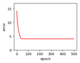
Figure 3. Without nonlinear activation functions.

There are many different variants of RNNs (Greff et al., 2016). Vanilla RNN (Mandic and Chambers, 2001), long short-term memory (LSTM) (Hochreiter and Schmidhuber, 1997) and gated recurrent unit (GRU) (Cho et al., 2014) are the most popular ones. LSTM and GRU are the extensions of vanilla RNN for handling long-term dependency problem. For simplicity, we focus on the vanilla RNN as other variants are built upon it. The extension to LSTM and GRU will be similar. The formalization of vanila RNN is as follows:

(1) $$\small\mathbf{h}_{t+1} =\tanh(W_{h}\mathbf{h}_{t}+W_{x}\mathbf{x}_{t+1}),$$

(2) $$\mathbf{y}_{t} =f(W_{o}\mathbf{h}_{t}),$$

where $W_{h}\in\mathbb{R}^{m\times m}$, $W_{x}\in\mathbb{R}^{m\times n}$, and $W_{o}\in\mathbb{R}^{l\times m}$ are the coefficient matrix. The activation function $f$ is chosen according to the task.

As the length of the historical records varies, the RNN that learns the vector addition should output the cumulative sum at each step. Thus, $\mathbf{y}_{t}$ should be the predicted sum of input $\mathbf{x}_{1},...,\mathbf{x}_{t}$. The corresponding ground truth is $\sum\limits_{i=1}^{t}\mathbf{x}_{i}$. As our goal is to learn a linear operation addition, the nonlinear layer is not necessary. Thus, we remove all the nonlinear layers and rewrite Formula 1 and 2 as follows:

(3) $$\small\mathbf{h}_{t+1} =W_{h}\mathbf{h}_{t}+W_{x}\mathbf{x}_{t+1},$$

(4) $$\mathbf{y}_{t} =W_{o}\mathbf{h}_{t},$$

If we recursively apply Equations 3 and 4, we obtain

(5) $$\small\mathbf{y}_{t} =\sum\limits_{i=1}^{t}W_{o}W_{h}^{t-i}W_{x}\mathbf{x}_{i},$$

where $\mathbf{h}_{0}$ is the initial state which is a zero vector. Thus, the closed-form solution is $W_{o}W_{x}=\mathbb{I}^{n\times n}=\mathbb{I}^{l\times l}$ and $W_{h}=\mathbb{I}^{m\times m}$. This closed-form solution indicates that the vanilla RNN can represent the vector addition without too many parameters if we can meet the constraints in the closed-form solution. A single layer RNN with hidden state of small dimensionality has enough representation ability. As the nonlinear activation function may affect the learning process, we also re-conduct the experiments to learn the vector addition with the simplified RNN version described by Equation 3 and  4. Other configurations are the same as before. The training process is shown in Figure 3. The training error still converges around 4. Thus, our results imply that the vanilla RNN has the ability to learn vector addition in theory, but in practice the optimizers cannot find this global minimal (or unable to do so in feasible time). To this end, we demonstrate the RNN based methods fail to capture PIF.

2.4.3. How to Overcome the Difficulty

The closed-form solution provides a direct solution to overcome this difficulty by initializing the parameters in the RNN with the optimal solution. However, the closed-form solution forces the weighted matrices to be correlated to each others, which violates the effect of random and orthogonal weight initializations. Recent literature shows that the neural networks trained by stochastic gradient descent (SGD) from random initialization almost never suffer from non-smoothness or non-convexity, and can avoid local minima (Goodfellow et al., 2014). And orthogonal weight initializations improve the convergence (Hu and Pennington, 2020). Even though our closed-form solution is easy for the RNNs to learn the vector addition, it brings difficulty in training the RNNs to learn other objectives, e.g. temporal dynamics which is also important in NBR. We believe the solution to overcome the difficulty in training RNNs from the optimization perspective is not trivial. So we think PIF should be carefully captured as it is hard to learn PIF with RNNs.

3. Proposed Method

Model-based methods have been considered as better solution for traditional collaborative filter recommendation problem than neighbor-based methods as model-based methods can better generalize to unseen patterns (Ning et al., 2015). However, our empirical results in section  2.2 show that the unseen patterns only account for a small part in the target basket. Thus, we propose to resort to the classical and direct neighbor-based methods. To our best knowledge, even though kNN methods have been developed in collaborative filter for top $n$ recommendation (Konstan et al., 1997)(Deshpande and Karypis, 2004) and sequential/session recommendation (Jannach and Ludewig, 2017), the kNN based method for NBR has not been explored. We will leave the model-based methods as our future work.

In the following, we introduce a simple and effective kNN based method called temporal-item-frequency-based user-KNN (TIFU-KNN). The proposed method directly utilizes the two important patterns associated with PIF. In addition, temporal dynamics is also considered to help select the items.

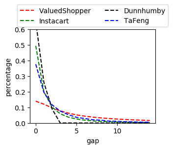
Figure 4. Gap distribution of repeated purchase.

3.1. Integrating Temporal Dynamics

Figure 5. User vector representation generation process.

PIF contains important information as we discuss in Section 2.2. However, there is a limitation: it cannot provide discriminative information for items with the same item frequency. Consequently, it is hard to distinguish items only with item frequency, which affects both neighbors searching and items selection in kNN-based method. To address this issue, we propose to consider the temporal dynamics of the repeated purchase. Figure 4 shows the gap distribution of repeated purchase on four data sets used in our experiments. The gap value means that after how many baskets, the next purchase for the same item occurs again. We can observe that the short gaps dominate the repeated purchase. However, the gap distribution varies dramatically across different data sets. For ValuedShopper data set, the percentage of different gaps decreases slowly while other three data sets decreases faster. Generally, we can observe that recent purchases have more impact to trigger a repeated purchase than the behavior long time ago. Thus, we propose to assign decayed weights to the same item appearing at different time steps. The earlier the item appears, the smaller weight the item contributes to the final frequency. We will describe the details in the next section.

3.2. Nearest Neighbors based Method

Our kNN method consists of two parts: the similarity calculation (between the target user and other users) and the prediction (based on the target user and his neighbors).
User Similarity Calculation: Considering each user’s historical records are sequential sets of variable length, we propose to aggregate the historical records into one vector which is easy for similarity calculation. The direct way to aggregate the historical records is to sum them up. But this way has a limitation that we have shown in the last section. Also, it ignores that the users’ preferences for products are drifting over time (Koren, 2009). This drifting suggests that recent records have more impact than the records long time ago. Thus, we make the items bought recently contribute more in the similarity calculation than the items bought long time ago. However, a single time decayed weight is not flexible to model another property of temporal dynamics that consecutive steps have small changes while steps far from each others have large changes. To capture both temporal dynamics, we propose to use hierarchical time decayed weights. Our user vector representation generation process is as follows (which is shown in the Figure 5):
(1) We partition the historical $t$ baskets (vectors) into $m$ groups equally. Denote the group size as $x=\frac{t}{m}$. The $j$-th vector (in temporal order) within each group is multiplied by a time-decayed weight $r_{b}^{x-j}$, where $r_{b}$ is the time-decayed ratio within group. Then, we calculate the average vector of the weighted vectors within each group as the corresponding group vector $\mathbf{v}_{group}$. If the vectors cannot be equally partitioned, the group size $x$ is calculated by $\lceil\frac{t}{m}\rceil$ except for the first group whose size is $t-x\cdot(m-1)$.
(2) The $i$-th group vector $\mathbf{v}_{group_{i}}$ is multiplied by a time-decayed weight $r_{g}^{m-i}$, where $r_{g}$ is the time-decayed ratio across the groups. Then, we calculate the average vector of the weighted group vectors as the user vector representation $\mathbf{u}$.

After we obtain the user vector representation, we can use different methods (Sarwar et al., 2001) to calculate the similarity. Here we use the Euclidean distance to help calculate the similarity between users. The small(large) distance means large(small) similarity. We will leave the exploration of other similarity functions as our future work. We search the $k$ nearest neighbors for each target user.
Prediction: Our prediction is a combination of following two parts:

• Repeated purchase component: Denote the user representation of the target user as $\mathbf{u_{t}}$. It is corresponding to repeated purchase pattern.

• Collaborative purchase component: Denote the set of target user’s nearest neighbors vector representations as $U_{neighbor}$. Denote the average vector of all vectors belong to $U_{neighbor}$ as $\mathbf{u_{n}}$. $\mathbf{u_{n}}$ is corresponding to collaborative purchase pattern.

The final prediction is:

$$\mathbf{P}=\alpha\cdot\mathbf{u_{t}}+(1-\alpha)\cdot\mathbf{u_{n}},$$

where the $\alpha$ is a hyper-parameter to balance two parts. The $s$ items corresponding to the largest $s$ entries in $\mathbf{P}$ are recommended.

4. Related Work

The related works include (1) Traditional collaborative recommendation methods that model user preferences without considering the temporal dynamics and have a set of items as the historical record; (2) Sequential recommendation methods that deal with a sequence of items or actions (each element is an item or action) as the user profile; and (3) NBR methods that deal with a sequence of baskets (each element is a set of items) as the user profile.
Traditional collaborative recommendation: Collaborative Filtering (CF) (Ricci et al., 2011) is the classical recommendation method. CF usually learns from user-item ratings matrix and predict only based on this matrix. Existing CF methods can be classified into two categories: neighborhood- and model-based methods. Neighborhood-based methods are widely studied in traditional collaborative recommendation (Ning et al., 2015). The neighborhood-based methods contain two ways: user-based or item-based recommendation. User-based method like GroupLens (Konstan et al., 1997) predicts the interest of a target user for an item using the ratings for this item by the most similar users. The item-based method like itemKNN (Deshpande and Karypis, 2004) predicts the user-item rating based on the ratings of the target user for similar items. Model-based approaches use these ratings to learn a predictive model (Koren, 2008)(Bell et al., 2007). Recently, neural networks-based methods are proposed to enhance the CF methods (He et al., 2017)(Liang et al., 2018)(He et al., 2020) as more nonlinear relations can be captured by neural networks.
Sequential recommendation: The goal of sequential recommendation is to recommend the next item or action based on the past sequence of items (He and McAuley, 2016)(Kang and McAuley, 2018)(He et al., 2018)(Yuan et al., 2020). Due to the sequence structure in the historical records, natural language processing methods, like RNNs, attention mechanism, and Markov chain, can be applied to model the data (He and McAuley, 2016)(Kang and McAuley, 2018)(Hidasi et al., 2015). Session-based Recommendation also belongs to this type as each session is a short sequence of behaviors or items (Ludewig and Jannach, 2018)(Jannach and Ludewig, 2017). A kNN-based method shows competitive performance when it is compared to RNN-based method GRU4rec (Jannach and Ludewig, 2017). Our kNN-based method is different from this method in both similarity calculation step and prediction step. Also, their method cannot be directly applied to NBR as discussed in the introduction.
Next-basket recommendation: NBR aims at predicting a set of items based on a sequence of past baskets (sets) (Rendle et al., 2010)(Wang et al., 2015)(Yu et al., 2016)(Ying et al., 2018)(Bai et al., 2018)(Hu and He, 2019). The summary can be found in section 2.3. Unlike traditional collaborative recommendation and sequential recommendation, the study towards kNN-based method on NBR is lacked. There is no clue if this type of methods can provide better performance. Our proposed kNN-based method fills this gap.
Difficulty in Training RNNs: The vanishing and the exploding gradient problems are the well-known difficulty in training RNNs  (Pascanu et al., 2013). We present another phenomenon that it is difficult for RNNs to learn a simple operation—vector addition. Even though we know training a deep neural network is np-complete in the worst case (Blum and Rivest, 1989), the phenomenon discovered in this paper is different as we provide a closed-form solution. There is a need for more theoretical analysis to understanding this kind of difficulty in training RNNs.

5. Experiments

In this section, we conduct extensive experiments to answer the following research questions:
RQ1: How is the effectiveness of the proposed methods? Can they outperform the state-of-the-art NBR methods?
RQ2: How is the effectiveness of the temporal dynamics?
RQ3: How is the effectiveness of each component to predict the target basket in the TIFU-KNN?
RQ4: How do the hyper parameters affect the performance? Does each factor in the TIFU-KNN bring benefits?

5.1. Experimental Settings

5.1.1. Data sets

We use four public data sets: Dunnhumby, ValuedShopper, Instacart, and TaFeng. These data sets contain the transactions about which items are bought by which customer at which time. All the items bought in the same order are treated as a basket. We remove all the customers who have baskets less than 3 to ensure that temporal patterns exist in the past records. In Dunnhumby, we use the 50k users sampled data. In ValuedShopper data set, we use the sampled transactions data. In Instacart and TaFeng data sets, we remove the least frequent items. The left items retain more than 95% item purchase of all the transactions. The statistics of the data sets after pre-processing is shown in the Table 2.

Table 2. Statistic information after pre-processing.

Data	#items	#users	average basket size	average #baskets /user
ValuedShopper	7,907	10,000	8.71	56.85
Instacart	8,000	19,935	8.97	7.97
Dunnhumby	4,997	36,241	7.33	7.99
TaFeng	12,062	13,949	6.27	5.69

5.1.2. Evaluation Protocol

We use recall and NDCG to evaluate our methods. Recall is a wildly-used measurement in the NBR (Ying et al., 2018). NDCG is a ranking based measure which takes into account the order of elements in a list (He et al., 2015). We calculate the NDCG for each basket based on the top $s$ sorted elements list. All the measurements are calculated across all predicted next set of items.

We use the past baskets of a given customer to predict his/her last basket. All the data sets are partitioned across users. The data is randomly partitioned into 5 folds across users. And 4 folds is used for training and 1 fold is used for test. We reserve the data of 10% users in the training set as the validation set for hyper parameters searching in all the methods.

5.1.3. Compared Methods

Simple baselines:

• Top-$n$ frequent (TopFreq): It uses the most frequent $s$ items that appear in all the baskets of the training data as the predicted next baskets for all persons.

• Personalized Top-$n$ frequent (PersonTopFreq): It uses the most frequent $s$ items that appear in the past baskets of a given person as the prediction for the next basket. It directly use the PIF.

Tweaked methods:

• userKNN: It is classical collaborative filter based on kNN (Konstan et al., 1997). In order to apply this method, we merge all the items in the historical baskets as a set of items. We recommend the top $s$ items as the next basket. This baseline can show the difference between the proposed method and the existing user-based kNN method.

• RepeatNet: The latest RNN-based model for session-based recommendation which captures the repeated behaviors (Ren et al., 2019). To apply this method to solve our problem, we transfer each basket into a sequence based on the ID’s order. Then, we concatenate the sequences from different baskets in temporal order and get a sequence of items for each user.

Existing NBR methods:

• FPMC: The classical factorization based method for next basket recommendation. It use Markov chain and factorization method to represent the past baskets (Rendle et al., 2010). Both sequential behaviors and users’ personal tastes are taken into account for prediction.

• DREAM: A deep model based on embedding and RNN for next basket recommendation (Yu et al., 2016). It considers personal dynamic interests at different time and the global interactions of all baskets of the user over time.

• SHAN: A deep model based on hierarchical attention networks (Ying et al., 2018) . It partitions the historical baskets into long-term and short-term parts to learn the long-term preference and short-term preference based on the corresponding items attentively. It can be directly applied in NBR and sequential/session-based recommendation as it treats the historical records as two sets.

• Sets2Sets: The state-of-the-art end-to-end method for following multiple baskets prediction based on RNN (Hu and He, 2019). Repeated purchase pattern is also integrated into the method.

We focus on comparing with existing NBR methods. Other techniques used in top $n$ recommendation and sequential/session-based recommendation are not the focus of this paper.

Table 3. Parameters of our methods in different data sets.

Data	$k$	$m$	$r_{b}$	$r_{g}$	$\alpha$
ValuedShopper	300	7	1	0.6	0.7
Instacart	900	3	0.9	0.7	0.9
Dunnhumby	900	3	0.9	0.6	0.2
TaFeng	300	7	0.9	0.7	0.7

Table 4. Comparison with different methods. The bold is the maximum in (a)-(b). The underline is the maximum in (c)-(h).

Data	Metric	(a)	(b)	(c)	(d)	(e)	(f)	(g)	(h)	(i)	improvement vs.
		TopFreq	PersonTopFreq	userKNN	RepeatNet	FPMC	DREAM	SHAN	Sets2Sets	TIFU-KNN	(a)-(b)	(c)-(h)
ValuedShopper	recall@10	0.0982	0.2109	0.0988	0.1031	0.0951	0.0991	0.0847	0.1259	0.2162	2.5%	71.7%
	recall@20	0.0904	0.2969	0.1329	0.1485	0.1391	0.1448	0.1220	0.1774	0.3028	2.7%	70.6%
	NDCG@10	0.0779	0.2128	0.1415	0.1439	0.1188	0.1231	0.1032	0.1626	0.2171	2.1%	33.5%
	NDCG@20	0.0904	0.2544	0.1662	0.1693	0.1253	0.1287	0.1074	0.1884	0.2589	1.7%	37.4%
Instacart	recall@10	0.0724	0.3426	0.0720	0.2107	0.0763	0.0866	0.0902	0.3021	0.3952	15.3%	30.8%
	recall@20	0.1025	0.4652	0.1260	0.2637	0.1073	0.1128	0.1246	0.3654	0.4875	4.8%	33.4%
	NDCG@10	0.0641	0.3618	0.1020	0.2285	0.0946	0.1063	0.1152	0.3487	0.3825	5.7%	9.6%
	NDCG@20	0.0689	0.4155	0.1394	0.2513	0.0992	0.1157	0.1212	0.3626	0.4384	5.5%	20.9%
Dunnhumby	recall@10	0.0819	0.1853	0.1135	0.1324	0.0919	0.0915	0.1007	0.2068	0.2087	12.6%	0.9%
	recall@20	0.1077	0.2366	0.1648	0.1989	0.1186	0.1087	0.1201	0.2653	0.2692	13.7%	1.4%
	NDCG@10	0.0601	0.1771	0.1707	0.1545	0.1025	0.1009	0.1149	0.2134	0.1983	11.9%	-7.0%
	NDCG@20	0.0609	0.2016	0.2052	0.1732	0.1057	0.1022	0.1167	0.2385	0.2302	14.1%	-3.5%
TaFeng	recall@10	0.0773	0.0704	0.1089	0.0645	0.0868	0.0902	0.0878	0.1190	0.1301	33.7%	9.3%
	recall@20	0.1151	0.1203	0.1278	0.0919	0.1056	0.1149	0.1065	0.1767	0.1810	50.4%	2.4%
	NDCG@10	0.0519	0.0766	0.0832	0.0592	0.0667	0.0763	0.0813	0.0844	0.1011	31.9%	8.4%
	NDCG@20	0.0608	0.0896	0.1064	0.0679	0.0743	0.0841	0.0892	0.1071	0.1206	34.5%	12.6%

We tune the hyper parameters in all the compared methods with grid search to achieve their best performance. For userKNN, the number of nearest neighbors is searched from the set of values [100, 300,500, 700, 900, 1100, 1300]. For FPMC, the dimension of factor is searched from the set of values [16, 32, 64, 128]. For RepeatNet, DREAM, SHAN, and Sets2Sets, the embedding size is searched from the set of values [16, 32, 64, 128].

5.1.4. Configuration of the Proposed Method

We perform an extensive search over the parameter space to achieve the best performance on the validation set. The number of nearest neighbors $k$ is chosen from the set of values [100, 300, 500, 700, 900, 1100, 1300]. The the within-basket time-decayed ratio $r_{b}$ and the group time-decayed ratio $r_{g}$ are chosen from the set of values [0.1, 0.2, 0.3, 0.4, 0.5, 0.6, 0.7, 0.8, 0.9, 1]. The fusion weight $\alpha$ is searched from the set of values [0, 0.1, 0.2, 0.3, 0.4, 0.5, 0.6, 0.7, 0.8, 0.9, 1]. The number of groups $m$ is searched from the set of values [3, 7, 11, 15, 19, 23] in ValuedShopper data set and from the set of values [2, 3, 4, 5, 6, 7] in other data sets, respectively. The parameters associated with the results reported in the methods comparison are shown in the Table 3.

5.2. Performance Comparison (RQ1)

The comparisons with baselines and existing methods are shown in the Table 4. Several observations can be made. First, the simple top-$n$ frequent baseline achieves reasonable performance compared to other existing methods in recall. It indicates that some popular items are commonly purchased by different users. But this simple baseline almost produces the worst performance across different data sets. It implies that users also have their distinct items which cannot be obtained through this simple baseline.

Second, personalized top-$n$ frequent method achieves competitive performance across all data sets. This verifies that the impact of the repeated purchase pattern from the target users plays an important role in the prediction.

Third, the existing NBR methods (excluding Sets2Sets) is surpassed by the baseline personalized top-$n$ frequent method in ValuedShopper, Instacart, and Dunnhumby data sets by a large margin. The reason is that existing methods (excluding Sets2Sets) cannot capture PIF. Even though Sets2Sets captures PIF explicitly, it is still worse than the personalized top-$n$ frequent method in first two data sets. We believe the reason is that the learned coefficients cannot perfectly control Sets2Sets to rely on the PIF and RNN based module.

Fourth, the tweaked top-$n$ recommendation method userKNN and session-based recommnedation method RepeatNet are worse than the state-of-the-art method Sets2Sets. The reason is that they ignore the important information existing in the sequential sets. For userKNN, it discards the PIF. RepeatNet outperforms other method without repeated purchase pattern when the repeated purchase affects a lot in the data (excluding TaFeng data set). But it performs worse than other methods with repeated purchase pattern (personalized top-$n$ frequent baseline and Sets2Sets) as it also captures the non-existing order among the items within each basket.

Fifth, the proposed TIFU-KNN is better than other methods in ValuedShopper, Instacart and TaFeng data sets, which verifies the superiority of the proposed method. There is an exception in Dunnhumby data set that Sets2Sets achieves better NDCG while the proposed method achieves a little better recall. We believe the reason is that the embedding method used in Sets2Sets can help generalize to some unseen user-item patterns in the training set beyond the repeated purchase pattern and collaborative purchase pattern. It is consistent with our analysis in the section 2.2 that Dunnhumby has much more unseen patterns than other three data sets.

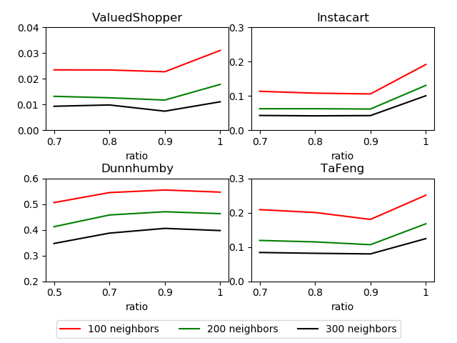
Figure 6. $Recall_{\overline{P}\cap\overline{N}}$ distribution on different data sets. The $r_{b}$ and $r_{g}$ are set to the same ratio. Different lines represent different numbers of neighbors.

5.3. Effectiveness of Temporal Dynamics (RQ2)

In this section, we investigate if the temporal dynamics brings positive effectiveness. For simplicity, we set the time decayed weights $r_{b}$ and $r_{g}$ to the same ratio. We denote the set of the nonzero entries in repeated purchase component and collaborative purchase component as $P$ and $N$, respectively. Then, we use the items in $\overline{P}\cap\overline{N}$ to retrieve items in the target basket and calculate the recall $Recall_{\overline{P}\cap\overline{N}}$. $Recall_{\overline{P}\cap\overline{N}}$ quantifies the amount of unseen patterns. The small value means large coverage by the repeated purchase pattern and collaborative purchase pattern. From Figure 6, we can observe that without the temporal dynamics, which is represented by $ratio=1$, the proposed method usually has the largest number of unseen patterns. It implies that the temporal dynamics can help reduce the unseen patterns as better neighbors are searched.

5.4. Effectiveness of Different Components (RQ3)

In this section, we investigate the contributions from two patterns associated with PIF. The comparison between our full TIFU-KNN and a single component as prediction is shown in the Table 5. Obviously, the combination achieves the best performance, which verifies the effectiveness of the combination of the target user’s PIF and the most similar users’ PIF. Also, we observe that target user’s repeated purchase pattern dominates the prediction. The collaborative purchase pattern provides discriminative information to further improve the prediction.

Table 5. The effect of each component in the TIFU-KNN.

		recall@10			NDCG@10
Data	$\small\mathbf{u_{t}}$	$\small\mathbf{u_{n}}$	$\small\mathbf{u_{t}\&u_{n}}$	$\small\mathbf{u_{t}}$	$\small\mathbf{u_{n}}$	$\small\mathbf{u_{t}\&u_{n}}$
ValuedShopper	0.1801	0.1251	0.2161	0.1716	0.1287	0.2171
Instacart	0.3698	0.1290	0.3952	0.3686	0.1381	0.3825
Dunnhumby	0.2070	0.1344	0.2087	0.1968	0.1270	0.1983
TaFeng	0.0921	0.0904	0.1301	0.0891	0.0766	0.1011

5.5. Sensitivity of the Hyperparameters (RQ4)

In this section, we investigate how the hyper parameters affect the performance. When we investigate on one or two parameters, we set other parameters just as the value shown in Table 3. We report the recall on the test set in Instacart data set when the predicted basket size $s=20$. The results are shown in the Figure 7. As the decayed weights $r_{b}$ and $r_{g}$ may have some correlation, we investigate them together and the results are shown in the Table 6. We have several observations. First, all the hyperparameters should be chosen with a proper value in order to achieve the best performance. Second, the parameters selected with the validation set are close to the optimal configuration for the test set. Third, the two time decayed weights $r_{b}$ and $r_{g}$ should both be smaller than 1 in order to achieve the best performance. It verifies that our two-level decayed weight design is better than any single decayed weight.

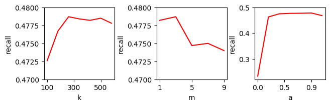
Figure 7. Sensitivity of hyperparameters: the number of nearest neighbors $k$, the number of groups $m$, and the combining weight $\alpha$ at Instacart data set.

Table 6. Sensitivity of hyperparameters: time-decayed ratio $r_{b}$ within each group and time-decayed ratio $r_{g}$ across the groups at Instacart data set.

recall			$\mathbf{r_{b}}$
$\mathbf{r_{g}}$	0.1	0.3	0.5	0.7	0.9	1
0.1	0.4504	0.4491	0.4474	0.4487	0.4497	0.4505
0.3	0.4754	0.4755	0.4751	0.4744	0.4694	0.4692
0.5	0.4786	0.4783	0.4783	0.4785	0.4782	0.4759
0.7	0.4837	0.4834	0.4832	0.4831	0.4841	0.4825
0.9	0.4869	0.4872	0.4874	0.4873	0.4878	0.4872
1	0.4780	0.4784	0.4778	0.4775	0.4772	0.4788

6. Conclusion

In this paper, we introduce a simple kNN-based method. Despite its simplicity, the proposed method generally outperforms the state-of-the art deep learning based methods. We study the reason why RNNs cannot approximate vector addition well, which provides the insight why our proposed method can outperform existing methods. Even though the deep learning model has strong representation power, there is no guarantee that we can find the solution which meets our expectation due to the complexity of non-convex optimization in RNNs. We believe this difficulty is different from the well-known vanishing and the exploding gradient problems  (Pascanu et al., 2013). More theoretical analysis is needed. A new optimizer that has the theoretical guarantee to find the global optimal like (Wang et al., 2019a) is also needed for RNNs.

Beyond this work, we believe that there are two directions that deserve to be explored. First, a direct extension is whether there are other commonly-used functions which are hard to be learned by existing widely-used deep models. This direction can help us better understand how to apply deep learning based methods in recommendation systems as we observe that recent publications (Ludewig et al., 2019) show a worry about the unclear progress in sequential/session-based recommendation. We believe different types of methods should have different advantages in different tasks and data sets. And a deep understanding about the boundary of the deep learning methods can bring benefits not only to recommendation systems but also to other machine learning areas. Second, another direct extension is to investigate if there are other patterns associated with PIF or other patterns that are associated with different types of item frequency, e.g., global item frequency, local item frequency (the item frequency associated with a small group of users or a small group of items), and inverse item frequency (Sharma and Karypis, 2019).
Acknowledgement: This research was supported part by NSF under grants CNS-1814322, CNS-1831140, CNS-1901103, US DoD DTRA DTRA grant HDTRA1-14-1-0040, and National Natural Science Foundation of China (61972372, U19A2079). Also, thanks to the constructive suggestions from the reviewers.

References

- (1)
- Aggarwal et al. (2016) Charu C Aggarwal et al. 2016. Recommender systems. Springer.
- Anderson et al. (2014) Ashton Anderson, Ravi Kumar, Andrew Tomkins, and Sergei Vassilvitskii. 2014. The dynamics of repeat consumption. In Proceedings of the 23rd international conference on World wide web. ACM, 419–430.
- Bai et al. (2018) Ting Bai, Jian-Yun Nie, Wayne Xin Zhao, Yutao Zhu, Pan Du, and Ji-Rong Wen. 2018. An attribute-aware neural attentive model for next basket recommendation. In The 41st International ACM SIGIR Conference on Research & Development in Information Retrieval. 1201–1204.
- Bell et al. (2007) Robert Bell, Yehuda Koren, and Chris Volinsky. 2007. Modeling relationships at multiple scales to improve accuracy of large recommender systems. In Proceedings of the 13th ACM SIGKDD international conference on Knowledge discovery and data mining. ACM, 95–104.
- Benson et al. (2016) Austin R Benson, Ravi Kumar, and Andrew Tomkins. 2016. Modeling user consumption sequences. In Proceedings of the 25th International Conference on World Wide Web. International World Wide Web Conferences Steering Committee, 519–529.
- Blum and Rivest (1989) Avrim Blum and Ronald L Rivest. 1989. Training a 3-node neural network is NP-complete. In Advances in neural information processing systems. 494–501.
- Bottou (2010) Léon Bottou. 2010. Large-scale machine learning with stochastic gradient descent. In Proceedings of COMPSTAT’2010. Springer, 177–186.
- Cho et al. (2014) Kyunghyun Cho, Bart Van Merriënboer, Dzmitry Bahdanau, and Yoshua Bengio. 2014. On the properties of neural machine translation: Encoder-decoder approaches. arXiv preprint arXiv:1409.1259 (2014).
- Dawes et al. (2015) John Dawes, Lars Meyer-Waarden, and Carl Driesener. 2015. Has brand loyalty declined? A longitudinal analysis of repeat purchase behavior in the UK and the USA. Journal of Business Research 68, 2 (2015), 425–432.
- Deshpande and Karypis (2004) Mukund Deshpande and George Karypis. 2004. Item-based top-n recommendation algorithms. ACM Transactions on Information Systems (TOIS) 22, 1 (2004), 143–177.
- Goodfellow et al. (2014) Ian J Goodfellow, Oriol Vinyals, and Andrew M Saxe. 2014. Qualitatively characterizing neural network optimization problems. arXiv preprint arXiv:1412.6544 (2014).
- Greff et al. (2016) Klaus Greff, Rupesh K Srivastava, Jan Koutník, Bas R Steunebrink, and Jürgen Schmidhuber. 2016. LSTM: A search space odyssey. IEEE transactions on neural networks and learning systems 28, 10 (2016), 2222–2232.
- He et al. (2018) Ruining He, Wang-Cheng Kang, and Julian McAuley. 2018. Translation-based Recommendation: A Scalable Method for Modeling Sequential Behavior.. In IJCAI. 5264–5268.
- He and McAuley (2016) Ruining He and Julian McAuley. 2016. Fusing similarity models with markov chains for sparse sequential recommendation. In 2016 IEEE 16th International Conference on Data Mining. IEEE, 191–200.
- He et al. (2015) Xiangnan He, Tao Chen, Min-Yen Kan, and Xiao Chen. 2015. Trirank: Review-aware explainable recommendation by modeling aspects. In Proceedings of the 24th ACM International on Conference on Information and Knowledge Management. ACM, 1661–1670.
- He et al. (2020) Xiangnan He, Kuan Deng, Xiang Wang, Yan Li, Yongdong Zhang, and Meng Wang. 2020. LightGCN: Simplifying and Powering Graph Convolution Network for Recommendation. In The 43st International ACM SIGIR Conference on Research & Development in Information Retrieval.
- He et al. (2017) Xiangnan He, Lizi Liao, Hanwang Zhang, Liqiang Nie, Xia Hu, and Tat-Seng Chua. 2017. Neural collaborative filtering. In Proceedings of the 26th International Conference on World Wide Web. International World Wide Web Conferences Steering Committee, 173–182.
- Hidasi et al. (2015) Balázs Hidasi, Alexandros Karatzoglou, Linas Baltrunas, and Domonkos Tikk. 2015. Session-based recommendations with recurrent neural networks. arXiv preprint arXiv:1511.06939 (2015).
- Hochreiter and Schmidhuber (1997) Sepp Hochreiter and Jürgen Schmidhuber. 1997. Long short-term memory. Neural computation 9, 8 (1997), 1735–1780.
- Hu and He (2019) Haoji Hu and Xiangnan He. 2019. Sets2Sets: Learning from Sequential Sets with Neural Networks. In Proceedings of the 25th ACM SIGKDD International Conference on Knowledge Discovery and Data Mining. ACM, 1491–1499.
- Hu and Pennington (2020) Wei Hu and Jeffrey Pennington. 2020. Provable Benefit of Orthogonal Initialization in Optimizing Deep Linear Networks. In International Conference on Learning Representations.
- Jacoby and Kyner (1973) Jacob Jacoby and David B Kyner. 1973. Brand loyalty vs. repeat purchasing behavior. Journal of Marketing research 10, 1 (1973), 1–9.
- Jannach and Ludewig (2017) Dietmar Jannach and Malte Ludewig. 2017. When recurrent neural networks meet the neighborhood for session-based recommendation. In Proceedings of the Eleventh ACM Conference on Recommender Systems. ACM, 306–310.
- Kang and McAuley (2018) Wang-Cheng Kang and Julian McAuley. 2018. Self-attentive sequential recommendation. In 2018 IEEE International Conference on Data Mining (ICDM). IEEE, 197–206.
- Kingma and Ba (2014) Diederik P Kingma and Jimmy Ba. 2014. Adam: A method for stochastic optimization. arXiv preprint arXiv:1412.6980 (2014).
- Konstan et al. (1997) Joseph A Konstan, Bradley N Miller, David Maltz, Jonathan L Herlocker, Lee R Gordon, and John Riedl. 1997. GroupLens: applying collaborative filtering to Usenet news. Commun. ACM 40, 3 (1997), 77–87.
- Koren (2008) Yehuda Koren. 2008. Factorization meets the neighborhood: a multifaceted collaborative filtering model. In Proceedings of the 14th ACM SIGKDD international conference on Knowledge discovery and data mining. ACM, 426–434.
- Koren (2009) Yehuda Koren. 2009. Collaborative filtering with temporal dynamics. In Proceedings of the 15th ACM SIGKDD international conference on Knowledge discovery and data mining. ACM, 447–456.
- Liang et al. (2018) Dawen Liang, Rahul G Krishnan, Matthew D Hoffman, and Tony Jebara. 2018. Variational autoencoders for collaborative filtering. In Proceedings of the 2018 World Wide Web Conference on World Wide Web. International World Wide Web Conferences Steering Committee, 689–698.
- Ludewig and Jannach (2018) Malte Ludewig and Dietmar Jannach. 2018. Evaluation of session-based recommendation algorithms. User Modeling and User-Adapted Interaction 28, 4-5 (2018), 331–390.
- Ludewig et al. (2019) Malte Ludewig, Noemi Mauro, Sara Latifi, and Dietmar Jannach. 2019. Performance comparison of neural and non-neural approaches to session-based recommendation. In Proceedings of the 13th ACM Conference on Recommender Systems. ACM, 462–466.
- Mandic and Chambers (2001) Danilo P Mandic and Jonathon Chambers. 2001. Recurrent neural networks for prediction: learning algorithms, architectures and stability. John Wiley & Sons, Inc.
- Ning et al. (2015) Xia Ning, Christian Desrosiers, and George Karypis. 2015. A comprehensive survey of neighborhood-based recommendation methods. In Recommender systems handbook. Springer, 37–76.
- Pascanu et al. (2013) Razvan Pascanu, Tomas Mikolov, and Yoshua Bengio. 2013. On the difficulty of training recurrent neural networks. In International conference on machine learning. 1310–1318.
- Ren et al. (2019) Pengjie Ren, Zhumin Chen, Jing Li, Zhaochun Ren, Jun Ma, and Maarten de Rijke. 2019. RepeatNet: A repeat aware neural recommendation machine for session-based recommendation. In Proceedings of the AAAI Conference on Artificial Intelligence, Vol. 33. 4806–4813.
- Rendle et al. (2010) Steffen Rendle, Christoph Freudenthaler, and Lars Schmidt-Thieme. 2010. Factorizing personalized markov chains for next-basket recommendation. In Proceedings of the 19th international conference on World wide web. ACM, 811–820.
- Ricci et al. (2011) Francesco Ricci, Lior Rokach, and Bracha Shapira. 2011. Introduction to recommender systems handbook. In Recommender systems handbook. Springer, 1–35.
- Sarwar et al. (2001) Badrul Sarwar, George Karypis, Joseph Konstan, and John Riedl. 2001. Item-based collaborative filtering recommendation algorithms. In Proceedings of the 10th international conference on World Wide Web. 285–295.
- Sharma and Karypis (2019) Mohit Sharma and George Karypis. 2019. Adaptive matrix completion for the users and the items in tail. In The World Wide Web Conference. ACM, 3223–3229.
- Siegelmann and Sontag (1992) Hava T Siegelmann and Eduardo D Sontag. 1992. On the computational power of neural nets. In Proceedings of the fifth annual workshop on Computational learning theory. ACM, 440–449.
- Wan et al. (2018) Mengting Wan, Di Wang, Jie Liu, Paul Bennett, and Julian McAuley. 2018. Representing and Recommending Shopping Baskets with Complementarity, Compatibility and Loyalty. In Proceedings of the 27th ACM International Conference on Information and Knowledge Management. ACM, 1133–1142.
- Wang et al. (2019b) Chenyang Wang, Min Zhang, Weizhi Ma, Yiqun Liu, and Shaoping Ma. 2019b. Modeling Item-Specific Temporal Dynamics of Repeat Consumption for Recommender Systems. In The World Wide Web Conference. 1977–1987.
- Wang et al. (2019a) Gang Wang, Georgios B Giannakis, and Jie Chen. 2019a. Learning ReLU networks on linearly separable data: Algorithm, optimality, and generalization. IEEE Transactions on Signal Processing 67, 9 (2019), 2357–2370.
- Wang et al. (2015) Pengfei Wang, Jiafeng Guo, Yanyan Lan, Jun Xu, Shengxian Wan, and Xueqi Cheng. 2015. Learning hierarchical representation model for next-basket recommendation. In Proceedings of the 38th International ACM SIGIR conference on Research and Development in Information Retrieval. ACM, 403–412.
- Ying et al. (2018) Haochao Ying, Fuzhen Zhuang, Fuzheng Zhang, Yanchi Liu, Guandong Xu, Xing Xie, Hui Xiong, and Jian Wu. 2018. Sequential recommender system based on hierarchical attention networks. In the 27th International Joint Conference on Artificial Intelligence.
- Yu et al. (2016) Feng Yu, Qiang Liu, Shu Wu, Liang Wang, and Tieniu Tan. 2016. A dynamic recurrent model for next basket recommendation. In Proceedings of the 39th International ACM SIGIR conference on Research and Development in Information Retrieval. ACM, 729–732.
- Yuan et al. (2020) Fajie Yuan, Xiangnan He, Haochuan Jiang, Guibing Guo, Jian Xiong, Zhezhao Xu, and Yilin Xiong. 2020. Future Data Helps Training: Modeling Future Contexts for Session-based Recommendation. In Proceedings of The Web Conference 2020. 303–313.