Adaptive quadrature schemes for Bayesian inference via active learning

Abstract

We propose novel adaptive quadrature schemes based on an active learning procedure. We consider an interpolative approach for building a surrogate posterior density, combining it with Monte Carlo sampling methods and other quadrature rules. The nodes of the quadrature are sequentially chosen by maximizing a suitable acquisition function, which takes into account the current approximation of the posterior and the positions of the nodes. This maximization does not require additional evaluations of the true posterior. We introduce two specific schemes based on Gaussian and Nearest Neighbors bases. For the Gaussian case, we also provide a novel procedure for fitting the bandwidth parameter, in order to build a suitable emulator of a density function. With both techniques, we always obtain a positive estimation of the marginal likelihood (a.k.a., Bayesian evidence). An equivalent importance sampling interpretation is also described, which allows the design of extended schemes. Several theoretical results are provided and discussed. Numerical results show the advantage of the proposed approach, including a challenging inference problem in an astronomic dynamical model, with the goal of revealing the number of planets orbiting a star.

Keywords: Numerical integration; emulation; Monte Carlo methods; Bayesian quadrature; experimental design; active learning.

1 Introduction and brief overview

In this work, we consider the approximation of intractable integrals of type

$$I=\int_{\mathcal{X}}f({\bf x})\bar{\pi}({\bf x})d{\bf x},$$

where $f({\bf x})$ is a generic integrable function and $\bar{\pi}({\bf x})$ is a probability density function (pdf). These integrals usually appear in Bayesian inference problems where $\bar{\pi}({\bf x})$ represents the posterior distribution of the variable of interest given the observed data. In the next subsections, we briefly review several approaches presented in the literature, which are related to the methodology presented this work.

1.1 Main families of quadrature methods

With the term numerical integration, we refer to a broad family of algorithms for calculating definite integrals, and by extension, the term is also used to describe the numerical solution of differential equations. Although exact analytical solutions to integrals are always desirable, such “unicorns” are rarely available, specially in real-world systems. Indeed, many applications in signal processing, statistics, and machine learning inevitably require the approximation of intractable integrals [1, 2, 3]. In particular, Bayesian methods need the computation of posterior expectations which, generally, are analytically intractable [2, 4]. The term numerical quadrature (or simply quadrature) is employed as a synonym for numerical integration [1]. More specifically, a quadrature formula is often stated as a weighted sum of integrand evaluations at specified points (a.k.a., nodes or knots) within the domain of integration.
Deterministic quadratures. A first family of numerical integration methods are the deterministic quadrature rules. A subclass within this family is the Newton-Cotes quadrature rules [1]. The Newton-Cotes formulas are based on evaluating the integrand at equally spaced nodes and are obtained by substituting the integrand function with a corresponding polynomial interpolation. Smaller approximation errors can often be obtained by using the Gaussian quadratures, where the nodes are optimally placed [1, 5, 6]. However, their applicability is restricted to certain particular cases.
Monte Carlo (MC) methods. A second family is formed by stochastic quadrature rules based on MC sampling methods [2, 4], such as Markov chain Monte Carlo (MCMC) and importance sampling algorithms. In this framework, the nodes of the quadrature rules are randomly chosen. However, the resulting estimators often have a high variance, specially when the dimension of the problem grows.
Variance Reduction. A third family, formed by the variance reduction techniques [7, 2], combines elements of the first two classes. In order to reduce the variance of the corresponding Monte Carlo estimators, deterministic procedures are included within the sampling algorithms, e.g., conditioning, stratification, antithetic sampling, and control variates [7]. Other interesting examples are the Riemann-based approximations which are combinations of a Riemann quadrature and random sampling [2, Chapter 4.3]. The Quasi-Monte Carlo (QMC) algorithms can be also included in this family. In QMC, deterministic sequences of points are generated (based on the concept of low-discrepancy) and then used as nodes of the corresponding quadrature [3]. Several other combinations of the previous classes above, mixing determinism with random sampling schemes, can be found in the literature [8, 9, 10].
Bayesian quadrature (BQ). The BQ framework represents a fourth approach which employs Gaussian Process (GP) regression algorithms for approximating the integrand function (and, as a consequence, the resulting integral as well) [11, 12, 13]. In the last years, this approach has raised the interest of several authors. One problem with this approach is that, in some cases, a negative estimation of the marginal likelihood can be obtained. Some possible solutions have been proposed, although they are quite complex based on successive approximations [14, 15]. In this work, we provide two novel and much simpler alternatives for solving this issue. Moreover, unlike this work, most contributions in BQ literature focus on the GP approximation of the function $f({\bf x})$ [14, 15, 16], although other papers on BQ describe quite general frameworks where $f({\bf x})$ can contain the likelihood or $\pi({\bf x})$ [11, 12, 13]. A connection between classical quadratures and BQ can be found in [17]. Finally, theoretical guarantees for adaptive BQ schemes can be found in the insightful work of [18].

1.2 Emulation of complex models

Many Bayesian inference problems involve the evaluation of computationally intensive models, because of (i) the use of particularly complex systems or (ii) a large number of available data (or both). To overcome this issue, one possible strategy consists in replacing the true model by a surrogate model (a.k.a. an emulator), that could be also adaptively improved [19, 20, 21]. Then, Bayesian inference is carried out on this approximate, cheaper model.
Use of the emulator. The emulator can be applied mainly in three different ways. (a) One possibility is to apply MC sampling methods considering the surrogate model as the target pdf [22, 23]. This is used to speed up the MC algorithms. (b) In order to improve the efficiency of MC estimators, a second option is to use the emulator as a proposal density within an MC technique, as we discuss in Section 1.3 [24, 25, 26]. (c) A third possibility is to replace the true posterior with the emulator in the integrals of interest, and computing them [11, 12, 13]. Here, we mainly focus on the last approach, also combining it with MC methods (and other quadrature rules).
Construction of the emulator. In the literature, the surrogate model is often built by using a regression algorithm, like a GP model or similar techniques [27, 28]. This probabilistic approach provides also uncertainty quantification that is used for estimating the approximation error and adapting the emulator [29]. Sometimes, the approximation regards only some part of the model or is applied in a different domain (as the log-domain) [30, 31, 32, 33]. Other authors employ density estimation techniques for building the surrogate model, and then using it as a proposal density within MC algorithms [34, 35, 36] or for replacing the true posterior (again within MC methods) [37].

1.3 Interpolative proposal densities within Monte Carlo schemes

The first use of an interpolative procedure for building a proposal density is ascribable to the adaptive rejection sampling schemes [24, 38, 39, 40]. The proposal is formed by polynomial pieces (constant, linear, etc.). Several works have proposed the use of interpolative proposal densities within MCMC algorithms [25, 41, 42, 43]. For more details, see also [4, Chapters 4 and 7]. Their use within an importance sampling scheme is considered in [44]. The adaptation is carried out considering different statistical tests, by measuring the discrepancy between the emulator and the posterior [26].
The conditions needed for applying an emulator as an proposal density are discussed in [26]. For this purpose, we need to be able to: (a) update the construction of the emulator, (b) evaluate the emulator, (c) normalize the function defined by the emulator, and (d) draw samples from the emulator. It is not straightforward to find an interpolative construction which satisfies all those conditions jointly, for an arbitrary dimension of the problem. However, the resulting algorithms (when they can be applied) provide good performance, confirming that the interpolative approach deserves more attention.

1.4 Contributions

In this work, we leverage the advances in different fields of numerical integration and emulation, in order to design algorithms which build (a) better emulators and (b) more efficient quadrature rules. The novel algorithms are adaptive schemes which automatically select the nodes of the quadrature and of the resulting emulator. Namely, the set of nodes used by the emulator is sequentially updated by maximizing a suitable acquisition function. Below, we list the main contributions of the work.
$\bullet$ We propose a novel design of a suitable acquisition function defined as product of the posterior and a diversity term, taking into account the current positions of the nodes. Note that, unlike several works in the literature, e.g., [19, 45, 46, 20], we consider jointly both: the information regarding the posterior and the distances among the current nodes. For the selection of the nodes, some authors also consider the use of MCMC runs [22] or more sophisticated procedures combining sampling and deterministic quadrature schemes for selecting the nodes [47]. Unlike [22, 47], our adaptive approach is based on an active learning procedure. We also provide cheap versions of the acquisition function. The cheap acquisition functions do not require the evaluation of the posterior but only the evaluation of the emulator. The overall schemes are then parsimonious techniques which require the evaluation of the posterior density only at the nodes, sequentially selected by optimizing a cheap acquisition function. The proposed active learning strategy is also connected to the idea of obtaining a finite set of weighted representative points which can summarize, in some sense, a distribution. This topic has gained attention in the last years [48, 49, 50, 51].
$\bullet$ We consider an interpolative approximation of the posterior density $\bar{\pi}({\bf x})$, where the interpolant is expressed as a linear combination of generic kernel-basis functions. Unlike several BQ techniques in [14, 15, 16], we approximate $\bar{\pi}({\bf x})$ instead of the function $f({\bf x})$ in the integral $I$. For this purpose, we also propose the combination of the interpolant approach with MC and other quadrature schemes.
$\bullet$ With respect to other schemes in the literature [12, 13], our assumptions regarding the kernel-basis functions are less restrictive, e.g., they do not need to be symmetric. We could also employ different type of bases jointly, e.g., one different basis for each node. For instance, our framework allows the use of nearest neighbors (NN) basis functions, which presents several advantages: it does not require any matrix inversion and the coefficients of the linear combination (which defines the interpolator) are always positive [52], obtaining always a positive estimation of the marginal likelihood. These benefits are very appealing as shown in [14, 15, 53, 52].
$\bullet$ Section 5 presents an importance sampling (IS) interpretation of the proposed schemes, where the weights involve the interpolant instead of the true posterior density. This again shows that we can improve the Monte Carlo approximations without requiring additional evaluations of $\bar{\pi}({\bf x})$. Moreover, the alternative IS interpretation allows to design different techniques. One possible example is given in the final part of Section 5.
$\bullet$ We also introduce a novel procedure for fitting the bandwidth parameter of the Gaussian kernel in order to build an emulator of a density function. In this scenario, the proposed strategy performs better than the standard maximization of the marginal likelihood of the corresponding GP. Using this tuning procedure, we always obtain positive estimation of the marginal likelihood, even with Gaussian kernels (this is an important point; see [14, 15]).
We provide the theoretical support for the proposed methods in Section 7. Most of the convergence results are mainly known in the scattered data approximation literature [54, 55, 56]. The efficiency of the proposed schemes is also confirmed by several numerical experiments (in Section 8) with different target pdfs and dimensions of the problem. One of them is also a challenging astronomical application, where the goal is to detect the number of exoplanets orbiting a star, and infer their orbital parameters.

2 Interpolative quadratures for Bayesian inference

In many signal processing applications, the goal is to infer a variable of interest given a set of observations or measurements. Let us denote the variable of interest by ${\bf x}\in\mathcal{X}\subseteq\mathbb{R}^{d_{x}}$, and let ${\bf y}\in\mathbb{R}^{d_{y}}$ be the observed data. The posterior pdf is then

$$\bar{\pi}({\bf x})=p({\bf x}|{\bf y})=\frac{\ell({\bf y}|{\bf x})g({\bf x})}{Z({\bf y})},$$

where $\ell({\bf y}|{\bf x})$ is the likelihood function, $g({\bf x})$ is the prior pdf, and $Z({\bf y})$ is the model evidence (a.k.a. marginal likelihood). Generally, $Z({\bf y})$ is unknown, so we are able to evaluate the unnormalized target function,

$$\pi({\bf x})=\ell({\bf y}|{\bf x})g({\bf x}).$$

Usually, the analytical computation of the posterior density $\bar{\pi}({\bf x})\propto\pi({\bf x})$ is unfeasible, hence numerical approximations are required. Our goal is to approximate integrals of the form

$$I=\int_{\mathcal{X}}f({\bf x})\bar{\pi}({\bf x})d{\bf x}=\frac{1}{Z}\int_{\mathcal{X}}f({\bf x})\pi({\bf x})d{\bf x},$$ (1)

where $f({\bf x})$ is some integrable function, and

$$Z=\int_{\mathcal{X}}\pi({\bf x})d{\bf x}.$$ (2)

In the literature, random sampling or deterministic quadratures are often used [4, 57, 2]. In this work, we consider alternative quadrature rules based on an adaptive interpolative procedure. The adaptation is obtained by applying an active learning scheme.

2.1 Interpolative approach

Let us consider a set of distinct nodes ${\bf x}_{1},\dots,{\bf x}_{N}\in\mathcal{X}$ and some non-negative kernel or basis function, $k({\bf x},{\bf x}^{\prime}):\mathcal{X}\times\mathcal{X}\to\mathbb{R}^{+}\cup\{0\}$ (i.e., $k({\bf x},{\bf x}^{\prime})\geq 0$). From now on, we use the terms basis or kernel as synonyms. The interpolant of $\pi({\bf x})$ is as follows

$$\widehat{\pi}({\bf x})=\sum_{i=1}^{N}\beta_{i}k({\bf x},{\bf x}_{i}),$$ (3)

where the coefficients $\beta_{i}$ must be such that $\widehat{\pi}({\bf x})$ interpolates the points $\pi({\bf x}_{1}),\dots,\pi({\bf x}_{N})$, that is, $\widehat{\pi}({\bf x}_{i})=\pi({\bf x}_{i})$ for $i=1,\dots,N$. Hence, the $\beta_{i}$ are the solutions to the following linear system

$$\left\{\begin{split}&\beta_{1}k({\bf x}_{1},{\bf x}_{1})+....+\beta_{N}k({\bf x}_{1},{\bf x}_{N})=\pi({\bf x}_{1}),\\ &\beta_{1}k({\bf x}_{2},{\bf x}_{1})+....+\beta_{N}k({\bf x}_{2},{\bf x}_{N})=\pi({\bf x}_{2}),\\ &\qquad\vdots\\ &\beta_{1}k({\bf x}_{N},{\bf x}_{1})+....+\beta_{N}k({\bf x}_{N},{\bf x}_{N})=\pi({\bf x}_{N}).\end{split}\right.$$ (4)

Denoting $({\bf K})_{i,j}=k({\bf x}_{i},{\bf x}_{j})$ ($1\leq i,j\leq N$), $\bm{\beta}=[\beta_{1},\dots,\beta_{N}]^{\top}$ and ${\bf d}=[\pi({\bf x}_{1}),\dots,\pi({\bf x}_{N})]^{\top}$, Eq. (4) can be written in matrix form as ${\bf K}\bm{\beta}={\bf d}$. Thus, the coefficients are given by

$$\bm{\beta}={\bf K}^{-1}{\bf d}.$$ (5)

Note that, depending on the choice of kernel and its parameters, these coefficients can be negative.

Remark 1.

The only requirement regarding the functions $k({\bf x},{\bf x}^{\prime})$ is that the interpolation matrix ${\bf K}$ must be non-singular (i.e., invertible) for any set of distinct nodes. The symmetry of $k({\bf x},{\bf x}^{\prime})$ is not required. Different type of bases can be employed, for instance, one for each node ${\bf x}_{i}$, i.e., $k_{i}({\bf x},{\bf x}_{i})$.

Remark 2.

For simplicity, in this first part of the paper, we consider a fixed number of nodes $N$. However, a key point of the work is the adaptation procedure in Section 6, where new nodes are sequentially added.

A detailed theoretical analysis is provided in Section 7.

2.2 Interpolative quadrature schemes

We can approximate both $Z$ and $I$ by substituting the true $\pi({\bf x})$ with its interpolant $\widehat{\pi}({\bf x})$.
Approximation of $Z$. Let $\int_{\mathcal{X}}k({\bf x},{\bf x}_{i})d{\bf x}=C_{i}>0$ be the measure of the $i$-th kernel. An approximation of $Z$ can be obtained, by substituting Eq. (3) in (2),

$$\widehat{Z}=\int_{\mathcal{X}}\widehat{\pi}({\bf x})d{\bf x}=\sum_{i=1}^{N}\beta_{i}\int_{\mathcal{X}}k({\bf x},{\bf x}_{i})d{\bf x}=\sum_{i=1}^{N}\beta_{i}C_{i}.$$ (6)

If the kernels are normalized, i.e., $C_{i}=1$, note that $\widehat{Z}=\sum_{i=1}^{N}\beta_{i}$.

Remark 3.

Although $Z>0$, $\widehat{Z}$ can take negative values, since the coefficients $\beta_{i}$ can be negative. However, in this work, we suggest two schemes (with Gaussian bases and a suitable tuning procedure, and with NN bases) which ensure a positive estimation of $Z$.

Approximation of $I$. By substituting (3) and (6) in (1), we obtain an approximation of $I$ as

$$I\approx\widehat{I}=\frac{1}{\widehat{Z}}\int_{\mathcal{X}}f({\bf x})\widehat{\pi}({\bf x})d{\bf x}.$$ (7)

Note that, given $\widehat{\pi}({\bf x})=\sum_{i=1}^{N}\beta_{i}k({\bf x},{\bf x}_{i})$, the approximation of $I$ in (7) can be expressed as

$$\widehat{I}=\frac{1}{\widehat{Z}}\sum_{i=1}^{N}\beta_{i}\int_{\mathcal{X}}f({\bf x})k({\bf x},{\bf x}_{i})d{\bf x} =\frac{1}{\widehat{Z}}\sum_{i=1}^{N}\beta_{i}J_{i},$$ (8)

$$=\frac{1}{\widehat{Z}}\sum_{i=1}^{N}\nu_{i}\pi({\bf x}_{i}),$$

where $J_{i}=\int_{\mathcal{X}}f({\bf x})k({\bf x},{\bf x}_{i})d{\bf x}$, $\bm{\nu}=[\nu_{1},...,\nu_{N}]^{\top}={\bf K}^{-1}{\bm{\zeta}}$ with ${\bm{\zeta}}=[J_{1},\dots,J_{N}]^{\top}$ being the vector of integrals. Clearly, the performance of $\widehat{I}$ depends on the discrepancy between $\widehat{\pi}({\bf x})$ and $\pi({\bf x})$, as shown by Theorem 1. This discrepancy is reduced by properly adding new nodes, as suggested in Section 6.

2.3 Monte-Carlo based interpolative quadrature schemes

In this work, we assume that the evaluation of the target function $\pi({\bf x})$ is the main computational bottleneck [19, 21]. We consider that other operations, such as sampling and evaluating different proposal densities, are negligible with respect to the target evaluation. The techniques, presented in this section, do not require additional target evaluations with respect to Eq. (8). In some specific cases, we can compute the integrals $J_{i}$ and $C_{i}$ analytically (e.g., see next section). Otherwise, we need to approximate $J_{i}$, and in some cases, also $C_{i}$. Some general ideas are described below.
Normalized kernels ($C_{i}=1$). If the values $C_{i}=1$ are known, we can compute $\widehat{Z}=\frac{1}{N}\sum_{n=1}^{N}\beta_{i}$. Moreover, if we are able to draw samples from each $k({\bf x},{\bf x}_{i})$, we have

$$J_{i}=\int_{\mathcal{X}}f({\bf x})k({\bf x},{\bf x}_{i})d{\bf x}\approx\widehat{J}_{i}=\frac{1}{M}\sum_{m=1}^{M}f({\bf z}_{i,m}),$$ (9)

with ${\bf z}_{i,m}\sim k({\bf x},{\bf x}_{i})$, hence

$$\widehat{I}\approx\frac{1}{\widehat{Z}M}\sum_{i=1}^{N}\beta_{i}\sum_{m=1}^{M}f({\bf z}_{i,m}).$$ (10)

If we know $C_{i}$, another possible scenario is when we are not able to draw from $k({\bf x},{\bf x}_{i})$. In this case, we can employ the importance sampling (IS) procedure described below to approximate the integrals $J_{i}$.
Kernels with unknown $C_{i}$. In this case, we also have to approximate $\int_{\mathcal{X}}k({\bf x},{\bf x}_{i})d{\bf x}=C_{i}$. For this purpose, we can employ IS with proposal densities $q_{i}({\bf x})$, with $i=1,...,N$, obtaining

$$C_{i}\approx\widehat{C}_{i}=\frac{1}{M}\sum_{m=1}^{M}w_{i,m},$$ (11)

where the weights are $w_{i,m}=\frac{k({\bf z}_{i,m},{\bf x}_{i})}{q_{i}({\bf z}_{i,m})}$ and ${\bf z}_{i,m}\sim q_{i}({\bf x})$. Moreover, we also obtain

$$J_{i}\approx\widehat{J}_{i}=\frac{1}{M}\sum_{m=1}^{M}w_{i,m}f({\bf z}_{i,m}).$$ (12)

Replacing (11)-(12) into (8), the final estimator is given by

$$\widehat{I} \approx\frac{1}{\sum_{i=1}^{N}\beta_{i}\sum_{m=1}^{M}w_{i,m}}\sum_{i=1}^{N}\beta_{i}\sum_{m=1}^{M}w_{i,m}f({\bf z}_{i,m}),$$ (13)

$$=\sum_{m=1}^{M}\sum_{i=1}^{N}\bar{\rho}_{i,m}f({\bf z}_{i,m}),$$ (14)

where $\bar{\rho}_{i,m}=\frac{\beta_{i}w_{i,m}}{\sum_{j=1}^{N}\sum_{k=1}^{M}\beta_{j}w_{j,k}}$.

Remark 4.

Note that, in any of the scenarios above, we do not need to evaluate the target $\pi({\bf x})$ at the samples ${\bf z}_{i,m}$. Namely, we do not require additional target evaluations with respect to Section 2.2. Moreover, as $M\rightarrow\infty$, the estimators in Eqs. (10)-(14) converge to the expression (8), under standard MC arguments [2].

For further details, see the theoretical results in Section 7.2.2 and Theorems 6 and 7. So far we have considered Monte Carlo approaches to estimate $J_{i}$ and $C_{i}$. Other particular and more efficient approaches (such as deterministic quadratures) are possible if we consider specific kernel functions. In the next sections, we analyze two specific cases (with Gaussian and NN kernels).

3 Interpolation with Gaussian kernels

Let us consider the case of Gaussian kernels (with an unbounded support $\mathcal{X}=\mathbb{R}^{d_{x}}$),

$$k_{G}({\bf x},{\bf x}_{i})=$$

$$\frac{1}{(2\pi)^{\frac{d_{x}}{2}}|{\bf\Sigma}|^{\frac{1}{2}}}\exp\left(-\frac{1}{2}({\bf x}-{\bf x}_{i})^{\top}{\bf\Sigma}^{-1}({\bf x}-{\bf x}_{i})\right),$$ (15)

where ${\bf\Sigma}$ is a positive definite matrix. We take ${\bf\Sigma}=h^{2}{\bf I}$ where $h>0$ is the bandwidth hyperparameter that needs to be tuned (see Section 3.1). Alternatively, note that we can also use unnormalized Gaussian kernels $k_{G}({\bf x},{\bf x}_{i})=A\exp\left(-\frac{1}{2}({\bf x}-{\bf x}_{i})^{\top}{\bf\Sigma}^{-1}({\bf x}-{\bf x}_{i})\right)$, where $A$ is another parameter to possibly tune, and then consider $C_{i}=A(2\pi)^{\frac{d_{x}}{2}}|{\bf\Sigma}|^{\frac{1}{2}}$.
Polynomial functions $f({\bf x})$. The use of Gaussian kernel functions $k_{G}({\bf x},{\bf x}_{i})$ with $f({\bf x})$ being polynomial, ensures that the integrals in (8) are available in closed-form. Let ${\bf f}({\bf x})={\bf x}^{r}=[x_{1}^{r},\dots,x_{d_{x}}^{r}]^{\top}$ be componentwise powers of ${\bf x}\in\mathbb{R}^{d_{x}}$ ($r=1,2,\dots$). Then,

$$J_{i}=\int_{\mathbb{R}^{d_{x}}}{\bf f}({\bf x})k_{G}({\bf x},{\bf x}_{i})d{\bf x}=\int_{\mathbb{R}^{d_{x}}}{\bf x}^{r}k_{\text{G}}({\bf x},{\bf x}_{i})d{\bf x},$$

corresponds to the $r$-th marginal moments of a multivariate Gaussian centered at ${\bf x}_{i}$. Note that the marginal moments of a Gaussian density are well-known. Some instances are

$$\int_{\mathbb{R}^{d_{x}}}{\bf x}k_{\text{G}}({\bf x},{\bf x}_{i})d{\bf x}={\bf x}_{i}\qquad(r=1),$$

$$\int_{\mathbb{R}^{d_{x}}}{\bf x}^{2}k_{\text{G}}({\bf x},{\bf x}_{i})d{\bf x}={\bf x}_{i}^{2}+\text{diag}({\bf\Sigma}),\qquad(r=2),$$

where the power ${\bf x}_{i}^{2}$ is considered a componentwise operation. Then, in this case, we can directly replace the values of $J_{i}$ in Eq. (8).
Generic functions $f({\bf x})$. Each of the $N$ integrals on the right hand of (8) may be also approximated efficiently with a Gauss-Hermite quadrature (GH) [5, 6], i.e.,

$$\int_{\mathbb{R}^{d_{x}}}f({\bf x})k_{G}({\bf x},{\bf x}_{i})d{\bf x}\approx\widehat{J}_{i}=\sum_{m=1}^{M}\bar{w}^{\text{GH}}_{m}f({\bf z}_{i,m}),$$

where $\bar{w}^{\text{GH}}_{m}$ and ${\bf z}_{i,m}$ are the weights and nodes of the GH quadrature used for $i$-th integral. Note the quadrature weights are independent of $i$ and are normalized, i.e., $\sum_{m=1}^{M}\bar{w}^{\text{GH}}_{m}=1$. Moreover, we have ${\bf z}_{i,m}=\widetilde{{\bf z}}_{m}+{\bf x}_{i}$, that is, the only difference is a translation of a single set of GH nodes $\widetilde{{\bf z}}_{m}$ [6] (see also the Suppl. Material). Again, we do not need extra evaluations of the target $\pi({\bf x})$. Note that, with enough number of points ${\bf z}_{i,m}$, Gauss-Hermite quadrature is also exact when $f({\bf x})$ are polynomial functions [58]. Theoretical results, valid for positive definite radial basis functions, can be found in Section 7.2.

3.1 Probabilistic interpretation

If $k({\bf x},{\bf x}^{\prime})=k({\bf x}^{\prime},{\bf x})$ (i.e., it is symmetric) and $k({\bf x},{\bf x}^{\prime})$ is semi positive definite, as in the Gaussian case, we can interpret the construction of the interpolant $\widehat{\pi}({\bf x})$ as a Gaussian process (GP) [59]. In our setting, ${\bf d}=[\pi({\bf x}_{1}),\dots,\pi({\bf x}_{N})]^{\top}$ represents the observed vector. The process starts by placing a GP prior on $\pi({\bf x})$, $\pi({\bf x})\sim{\mathcal{GP}}({\bf 0},k({\bf x},{\bf x}^{\prime}))$, where the GP mean is ${\bf 0}$ and $k({\bf x},{\bf x}^{\prime})$ is the covariance function. Conditioning on d, it can be shown that the posterior of $\pi({\bf x})$ is given by

$$\pi({\bf x})|{\bf d}\sim\mathcal{GP}(\widehat{\pi}({\bf x}),C({\bf x},{\bf x}^{\prime})),$$

where the mean function is the interpolant $\widehat{\pi}({\bf x})$ given in (3), and the posterior covariance function is $C({\bf x},{\bf x}^{\prime})=k({\bf x},{\bf x}^{\prime})-{\bf k}({{\bf x}})^{\top}{\bf K}^{-1}{\bf k}({{\bf x}}^{\prime})$, with

$${\bf k}({{\bf x}})=[k({\bf x},{\bf x}_{1}),\dots,k({\bf x},{\bf x}_{N})]^{\top},$$

and $({\bf K})_{i,j}=k({\bf x}_{i},{\bf x}_{j})$. The variance at ${\bf x}$ is

$$V({\bf x})=C({\bf x},{\bf x})=k({\bf x},{\bf x})-{\bf k}({{\bf x}})^{\top}{\bf K}^{-1}{\bf k}({{\bf x}}).$$ (16)

Observe that $V({\bf x}_{i})=0$ for all $i=1,\dots,N$. If we assume that the vector of evaluations ${\bf d}$ is noisy, we can relax the exact fit requirement by introducing a regularization term, replacing ${\bf K}$ with the matrix ${\bf K}+\sigma^{2}{\bf I}$, where ${\bf I}$ is an $N\times N$ identity matrix. The noise term $\sigma^{2}$ also provides numerical stability. The probabilistic interpretation of the integrals involving $\pi$ is given in Appendix B.

3.2 Tuning of hyperparameters

Let us denote as $\bm{\theta}$ the vector as hyperparameters of the kernel functions $k({\bf x},{\bf x}^{\prime})$. A standard way of fitting the hyperparameters $\bm{\theta}$ is to maximize the marginal likelihood of the GP [59]. In this case, the evaluations of $\pi({\bf x})$ play the role of data. Given the evaluations ${\bf d}=[\pi({\bf x}_{1}),\dots,\pi({\bf x}_{N})]^{\top}$, the marginal likelihood is given by $p({\bf d}|\bm{\theta})=\mathcal{N}({\bf d}|{\bf 0},{\bf K})$, and its log-version is

$$\log p({\bf d}|\bm{\theta})=-\frac{1}{2}{\bf d}^{\top}{\bf K}^{-1}{\bf d}-\frac{1}{2}\log|{\bf K}|+c,$$

where $c$ is a constant. Note that ${\bf K}$ depends on $\bm{\theta}$. However, for fitting the bandwidth parameter $h$ of the Gaussian kernels, we propose an alternative procedure described in Appendix A, specifically designed for building an emulator of a density function. In this context, the proposed procedure performs better then the maximization of $p({\bf d}|\bm{\theta})$.

Remark 5.

Using the novel tuning procedure in Appendix A, the corresponding estimator $\widehat{Z}$ takes always positive values.

4 Constant kernels based on Nearest Neighbors

Given the set of nodes $\{{\bf x}_{i}\}_{i=1}^{N}$ in a bounded domain $\mathcal{X}$, consider now the use of constant kernels with finite support

$$k({\bf x},{\bf x}_{i})=\mathbb{I}_{\mathcal{R}_{i}}({\bf x}),$$ (17)

where $\mathbb{I}_{\mathcal{R}_{i}}({\bf x})$ is the indicator function in $\mathcal{R}_{i}$, i.e., $\mathbb{I}_{\mathcal{R}_{i}}({\bf x})=1$ for all $x\in\mathcal{R}_{i}$ and zero otherwise. Each $\mathcal{R}_{i}$ consists of the points ${\bf x}\in\mathcal{X}$ that are closest to ${\bf x}_{i}$, i.e.,

$$\mathcal{R}_{i}=\{{\bf x}\in\mathcal{X}:\left\lVert{\bf x}-{\bf x}_{i}\right\rVert_{p}\leq\min_{j\neq i}\left\lVert{\bf x}-{\bf x}_{j}\right\rVert_{p}\},$$

where $\left\lVert\cdot\right\rVert_{p}$ denotes the $p$-norm. That is, $\mathcal{X}=\cup_{i=1}^{N}\mathcal{R}_{i}$ is the Voronoi partition of $\mathcal{X}$ using $\{{\bf x}_{i}\}_{i=1}^{N}$ as support points. In this case, solving (5) for the coefficients $\bm{\beta}$ is straightforward since the matrix ${\bf K}$ is the identity matrix, and thus

$$\beta_{i}=\pi({\bf x}_{i})\enskip\text{for}\enskip i=1,\dots,N.$$

Note that all $\beta_{i}\geq 0$ with this kernel. Hence the interpolant is given by

$$\widehat{\pi}({\bf x})=\sum_{i=1}^{N}\pi({\bf x}_{i})\mathbb{I}_{\mathcal{R}_{i}}({\bf x}).$$ (18)

Note that to evaluate $\widehat{\pi}({\bf x})$ at any ${\bf x}$ we need to find just the closest node. We do not need to know the borders of regions $\{\mathcal{R}_{i}\}_{i=1}^{N}$ for this purpose. This choice of kernels has three clear advantages:

• no need to solve the linear system in (5) since ${\bf K}={\bf I}$ and hence $\bm{\beta}={\bf d}$,

• the coefficients $\bm{\beta}={\bf d}$ are always non-negative (this ensures that $\widehat{Z}\geq 0$),

• no need of tuning the bandwidth hyperparameter.

The difficulty, however, is determining the Voronoi partition, as well as the measures $C_{i}=\int_{\mathcal{X}}k({\bf x},{\bf x}_{i})d{\bf x}$. We show how to address these issues in Section 4.1. In this case,

$$C_{i}=\int_{\mathcal{X}}\mathbb{I}_{\mathcal{R}_{i}}({\bf x})d{\bf x}=|\mathcal{R}_{i}|,$$

where $|\mathcal{R}_{i}|$ denotes the measure of the $i$-th Voronoi region. The approximation of $Z$ is given by

$$\widehat{Z}=\sum_{i=1}^{N}\pi({\bf x}_{i})C_{i},$$ (19)

and Eq. (8) is expressed as

$$\widehat{I} =\frac{1}{\widehat{Z}}\sum_{i=1}^{N}\pi({\bf x}_{i})\int_{\mathcal{R}_{i}}f({\bf x})d{\bf x},$$

$$=\frac{1}{\sum_{k=1}^{N}\pi({\bf x}_{k})C_{k}}\sum_{i=1}^{N}\pi({\bf x}_{i})\int_{\mathcal{R}_{i}}f({\bf x})d{\bf x}.$$ (20)

The convergence of this scheme is guaranteed as $N$ grows, as shown by Theorems 8 and 9. Further theoretical analysis are provided in Section 7.3. Note that we need to estimate the measures $C_{i}$, as well as the integrals $\int_{\mathcal{R}_{i}}f({\bf x})d{\bf x}$ to compute $\widehat{Z}$ and $\widehat{I}$. The next section is devoted to this purpose.

4.1 Approximating Voronoi regions and resulting estimators

In order to approximate $C_{i}$, we can generate $M$ uniform vectors $\{{\bf z}_{m}\}_{m=1}^{M}$ in $\mathcal{X}$ via Monte Carlo sampling or Quasi-Monte Carlo sequences (e.g. a Sobol sequence) [57]. Define the set $\mathcal{U}_{i}$ as

$$\mathcal{U}_{i} =\{{\bf z}_{m}:\left\lVert{\bf z}_{m}-{\bf x}_{i}\right\rVert_{p}\leq\min_{j\neq i}\left\lVert{\bf z}_{m}-{\bf x}_{j}\right\rVert_{p}\}$$

$$=\{{\bf z}_{\ell_{i}}\}_{\ell_{i}=1}^{|\mathcal{U}_{i}|},$$

i.e., the $|\mathcal{U}_{i}|$ vectors closest to ${\bf x}_{i}$ in $p$-norm, which form a discrete approximation of $\mathcal{R}_{i}$. Note that $\sum_{i=1}^{N}|\mathcal{U}_{i}|=M$. Hence, the measure $C_{i}$ can be approximated by noting that $\frac{C_{i}}{|\mathcal{X}|}\approx\frac{|\mathcal{U}_{i}|}{M}$, hence

$$C_{i}\approx\frac{|\mathcal{U}_{i}|}{M}|\mathcal{X}|,$$ (21)

where $|\mathcal{X}|$ is the measure of $\mathcal{X}$. Thus, the estimator in Eq. (19) can be rewritten as

$$\widehat{Z} \approx\frac{|\mathcal{X}|}{M}\sum_{i=1}^{N}\pi({\bf x}_{i})|\mathcal{U}_{i}|.$$ (22)

We can also obtain an approximation of the integral $J_{i}=\int_{\mathcal{R}_{i}}f({\bf x})d{\bf x}$ by leveraging a QMC or MC approximation of the Voronoi regions. Specifically, the uniform vectors ${\bf z}_{\ell_{i}}$ in $\mathcal{U}_{i}$ can be used to approximate the integral in (4) as follows

$$J_{i}=\int_{\mathcal{R}_{i}}f({\bf x})d{\bf x} \approx\frac{C_{i}}{|\mathcal{U}_{i}|}\sum_{\ell_{i}=1}^{|\mathcal{U}_{i}|}f({\bf z}_{\ell_{i}})\approx\frac{|\mathcal{X}|}{M}\sum_{\ell_{i}=1}^{|\mathcal{U}_{i}|}f({\bf z}_{\ell_{i}}),$$ (23)

where we used (21) again in (23). The procedure above can be seen as an accept-reject method, and the estimators are also unbiased [4, Chapter 3 and Section 6.6]. Note that a simpler possible approximation with one point is $J_{i}=\int_{\mathcal{R}_{i}}f({\bf x})d{\bf x}\approx f({\bf x}_{i})C_{i}$. Thus, replacing the expressions (22)-(23) in (4), the final estimator becomes

$$\widehat{I} \approx\frac{1}{\sum_{k=1}^{N}\pi({\bf x}_{k})|\mathcal{U}_{k}|}\sum_{i=1}^{N}\pi({\bf x}_{i})\sum_{\ell_{i}=1}^{|\mathcal{U}_{i}|}f({\bf z}_{\ell_{i}}).$$ (24)

Connection with Section 2.3. The estimators above can be interpreted as the application of an importance sampling (IS) scheme as described in Section 2.3, for kernel functions with unknown $C_{i}$. However, unlike in Section 2.3, here we consider a unique and uniform proposal density

$$q_{i}({\bf x})=q({\bf x})=\frac{1}{|\mathcal{X}|}\mathbb{I}_{\mathcal{X}}({\bf x}),\qquad\forall i=1,...,N.$$

Then, we can also remove the subindex $i$ in the sample ${\bf z}_{i,m}\sim q({\bf x})$, i.e., we have only $M$ samples ${\bf z}_{m}\sim q({\bf x})$. Hence, following Eqs. (11)-(12), we have

$$C_{i} \approx\frac{1}{M}\sum_{m=1}^{M}w_{i,m},$$ (25)

$$J_{i}=\int_{\mathcal{R}_{i}}f({\bf x})d{\bf x} \approx\frac{1}{M}\sum_{m=1}^{M}w_{i,m}f({\bf z}_{m}),$$ (26)

where ${\bf z}_{m}\sim q({\bf x})=\frac{1}{|\mathcal{X}|}\mathbb{I}_{\mathcal{X}}({\bf x})$, and the weights are

$$w_{i,m}=\frac{k({\bf z}_{m},{\bf x}_{i})}{q({\bf z}_{m})}=\left\{\begin{split}&|\mathcal{X}|\quad\mbox{ if }\quad{\bf z}_{m}\in\mathcal{R}_{i},\\ &0\qquad\mbox{ if }\quad{\bf z}_{m}\notin\mathcal{R}_{i}.\\ \end{split}\right.$$ (27)

Replacing the expression of the weights $w_{i,m}$ into the formulas above, we recover the estimators in (22) and (24).

5 An alternative IS interpretation

In this section, we discuss a special case of the IS scheme given in Section 2.3, when a unique proposal $q_{i}({\bf x})=q({\bf x})$ is employed and only $M$ samples ${\bf z}_{m}\sim q({\bf x})$ are drawn (as already considered in the previous section). In this scenario, the IS procedure in Section 2.3 has another relevant interpretation, which allows us to design other different schemes. Considering a generic kernel $k({\bf x},{\bf x}_{i})$ and Eq. (25), we can rearrange $\widehat{Z}$ as

$$\widehat{Z}=\sum_{i=1}^{N}\beta_{i}C_{i} \approx\sum_{i=1}^{N}\beta_{i}\frac{1}{M}\sum_{m=1}^{M}w_{i,m}$$

$$=\sum_{i=1}^{N}\beta_{i}\frac{1}{M}\sum_{m=1}^{M}\frac{k({\bf z}_{m},{\bf x}_{i})}{q({\bf z}_{m})}$$

$$=\frac{1}{M}\sum_{m=1}^{M}\frac{\sum_{i=1}^{N}\beta_{i}k({\bf z}_{m},{\bf x}_{i})}{q({\bf z}_{m})}.$$

Then, recalling that $\widehat{\pi}({\bf x})=\sum_{i=1}^{N}\beta_{i}k({\bf x},{\bf x}_{i})$ and replacing this expression above, we finally obtain

$$\widehat{Z} \approx\frac{1}{M}\sum_{m=1}^{M}\frac{\widehat{\pi}({\bf z}_{m})}{q({\bf z}_{m})}=\frac{1}{M}\sum_{m=1}^{M}\gamma_{m},$$ (28)

where $\gamma_{m}=\gamma({\bf z}_{m})=\frac{\widehat{\pi}({\bf z}_{m})}{q({\bf z}_{m})}$ for $m=1,...,M$. Moreover, with similar steps, we can obtain

$$\widehat{I}\approx\frac{1}{M\widehat{Z}}\sum_{m=1}^{M}\gamma_{m}f({\bf z}_{m}),$$ (29)

Remark 6.

The weights $\gamma_{m}$ have the form of the standard IS weights with the target function $\widehat{\pi}$ in the numerator, and the proposal density $q$ in the denominator. Hence, the entire sampling procedure can be interpreted as a standard IS scheme where the target function is $\widehat{\pi}$ instead of $\pi$. This shows again that we do not need extra target evaluations and, hence, we can employ an arbitrary large value of $M$.

Remark 7.

Note that this result is valid for any kernel $k({\bf x},{\bf x}_{i})$, and we use a unique proposal $q({\bf x})$ in the procedure described in Section 2.3.

Below, we consider the NN case with a uniform proposal $q({\bf x})$, deriving the same formulas in Section 4.1.
Uniform proposal density and NN interpolator. Let us consider $q({\bf x})=\frac{1}{|\mathcal{X}|}\mathbb{I}_{\mathcal{X}}({\bf x})$, i.e., a uniform density in $\mathcal{X}$, and the NN kernel function. For each sample ${\bf z}_{m}$, the corresponding weight $\gamma_{m}$ is

$$\gamma_{m}=\gamma({\bf z}_{m})=\frac{\widehat{\pi}({\bf z}_{m})}{\frac{1}{|\mathcal{X}|}}=\frac{\pi({\bf x}_{k_{m}})}{\frac{1}{|\mathcal{X}|}}=|\mathcal{X}|\pi({\bf x}_{k_{m}}),$$

where ${\bf x}_{k_{m}}$ is the closest node to sample ${\bf z}_{m}$, i.e., ${\bf x}_{k_{m}}=\arg\min_{j}\left\lVert{\bf z}_{m}-{\bf x}_{j}\right\rVert_{p}$. Then, the IS approximation of $\widehat{Z}$ is

$$\widehat{Z}\approx\frac{1}{M}\sum_{m=1}^{M}\gamma_{m}=\frac{|\mathcal{X}|}{M}\sum_{m=1}^{M}\pi({\bf x}_{k_{m}})=\frac{|\mathcal{X}|}{M}\sum_{k=1}^{N}\pi({\bf x}_{k})|\mathcal{U}_{k}|,$$

where $|\mathcal{U}_{k}|$ counts the number of ${\bf z}_{m}$ whose closest node is ${\bf x}_{k}$ ($k=1,\dots,N$). Note that this expression is the same as in (22). Similarly, the IS estimate of $\widehat{I}$ is given by

$$\widehat{I}\approx\frac{1}{M\widehat{Z}}\sum_{m=1}^{M}\gamma_{m}f({\bf z}_{m}) =\frac{|\mathcal{X}|}{M\widehat{Z}}\sum_{m=1}^{M}\pi({\bf x}_{k_{m}})f({\bf z}_{m})$$

$$=\frac{|\mathcal{X}|}{M\widehat{Z}}\sum_{k=1}^{N}\pi({\bf x}_{k})\sum_{\ell_{k}=1}^{|\mathcal{U}_{k}|}f({\bf z}_{\ell_{k}}),$$

which is the same expression as in (24). However, this alternative IS interpretation allows us to design different schemes using a different proposal density, as shown below.
Gaussian mixture proposal. We consider now an alternative to the uniform proposal in $\mathcal{X}$. More specifically, we propose drawing $\{{\bf z}_{\ell}\}_{m=1}^{M}$ from a Gaussian mixture proposal pdf built considering the set of nodes $\{{\bf x}_{i}\}_{i=1}^{N}$, i.e.,

$${\bf z}_{m}\sim q({\bf x})=\sum_{i=1}^{N}\xi_{i}\mathcal{N}({\bf x}|{\bf x}_{i},{\bf C}_{i}),$$

where the mixture weights $\xi_{i}$ are

$$\xi_{i}=\frac{\pi({\bf x}_{i})}{\sum_{n=1}^{N}\pi({\bf x}_{n})},\qquad i=1,...,N,$$

and the covariances ${\bf C}_{i}$ can be determined by the minimum distance of ${\bf x}_{i}$ to its closest node. In this case, the IS weights are given by

$$\gamma({\bf z}_{m})=\frac{\widehat{\pi}({\bf z}_{m})}{\sum_{i=1}^{N}\xi_{i}\mathcal{N}({\bf z}_{m}|{\bf x}_{i},{\bf C}_{i})}=\frac{\pi({\bf x}_{k_{m}})}{\sum_{i=1}^{N}\xi_{i}\mathcal{N}({\bf z}_{m}|{\bf x}_{i},{\bf C}_{i})},$$

where ${\bf x}_{k_{m}}$ is the closest node to ${\bf z}_{m}$, with $m=1,\dots,M$.

(a) True target pdf

(b) $E=50$

(c) $E=250$

(d) $E=10^{3}$

Figure 1: Example of application of NN-AQ. The cross-marks represent the starting nodes, while the points added adaptively by NN-AQ are shown with dots. (a) The banana-shaped target and the starting nodes. (b)-(c)-(d) The NN-AQ emulator with $E=50,250,10^{3}$ number of target evaluations.

6 Adaptive procedure

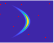
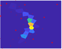
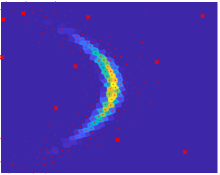
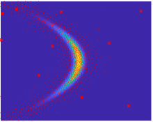
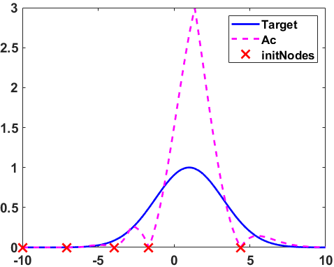
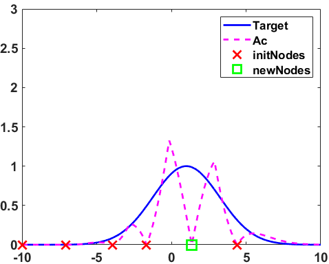
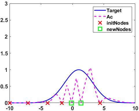
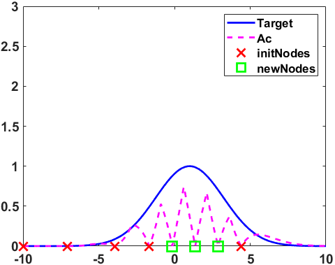
In this section, we present an adaptive mechanism to add new nodes to the interpolant. Our algorithm adds nodes sequentially with the aim to discover high-valued regions of $\pi({\bf x})$ while fostering the exploration of the state space. We employ an active learning procedure where a new point is obtained by maximizing a suitable acquisition function. The resulting adaptive algorithm is shown in Table 1. Note that the final number of nodes is $N_{T}=T+N_{0}$. The adaptive quadrature scheme based on the Gaussian kernels is denoted as GK-AQ, whereas the other scheme based on the Nearest Neighbors (NN) kernels is denoted as NN-AQ. Figure 1 depicts an example of application of the NN-AQ.

6.1 Building suitable acquisition functions

Let us denote as $t\in\mathbb{N}$ the $t$th iteration of the algorithm. In the update stage, we decide to add a new node where the acquisition function, $A_{t}:\mathcal{X}\to\{0\}\cup\mathbb{R}^{+}$, is maximum. The acquisition function takes into account the shape of ${\pi}({\bf x})$ and the spatial distribution of the current nodes. More specifically, it must fulfill

$$A_{t}({\bf x}_{i})=0\enskip\text{for all }t\mbox{ and }\enskip i=1,\dots,N_{t},$$

and grow as we move apart from the nodes. We consider acquisition functions $A_{t}({\bf x})$ of the form

$$A_{t}({\bf x})=\pi({\bf x})D_{t}({\bf x}),$$ (30)

where $D_{t}({\bf x})$ is a diversity term that penalizes the proximity to the current nodes. Note that the information of $f({\bf x})$ could be also included as $A_{t}({\bf x})=f({\bf x})\pi({\bf x})D_{t}({\bf x})$. In some settings, the function $A_{t}({\bf x})$ above could be directly used after choosing a diversity term $D_{t}({\bf x})$. However, in this work, we consider that evaluating $\pi({\bf x})$ is costly, so we propose cheaper versions of (30).

Table 1: Adaptive Quadrature algorithm.

Initialization: Set $N_{0}$ initial nodes and set ${\bf X}_{0}=\{{\bf x}_{1},\dots,{\bf x}_{N_{0}}\}$, ${\bf d}_{0}=[\pi({\bf x}_{1}),\dots,\pi({\bf x}_{N_{0}})]^{\top}$. For $t=0,\ldots,T$: 1. Build the interpolator. Use the set ${\bf X}_{t}=\{{\bf x}_{1},\dots,{\bf x}_{N_{t}}\}$ and corresponding evaluations ${\bf d}_{t}=[\pi({\bf x}_{1}),\dots,\pi({\bf x}_{N_{t}})]^{\top}$ to build $\widehat{\pi}_{t}({\bf x})$ using Gaussian kernels (see Section 3) or constant kernels (see Section 4). 2. Build the acquisition function. Use $\widehat{\pi}_{t}({\bf x})$ and the set of current nodes ${\bf X}_{t}$ to build the acquisition function $A_{t}({\bf x})$, e.g., Eqs. (33)-(34). 3. Update stage. Obtain new node ${\bf x}_{N_{t}+1}$ by $\displaystyle{\bf x}_{N_{t}+1}=\arg\max_{{\bf x}\in\mathcal{X}}A_{t}({\bf x}),$ (31) append ${\bf X}_{t+1}=\{{\bf X}_{t},{\bf x}_{N_{t}+1}\}$ and ${\bf d}_{t+1}=[{\bf d}_{t},\pi({\bf x}_{N_{t}+1})]^{\top}$. Outputs: Build the final interpolant $\widehat{\pi}_{T}({\bf x})$ and obtain the approximations $\widehat{I}$ and $\widehat{Z}$.

(a) Initial state

(b) Iteration 1

(c) Iteration 2

(d) Iteration 3

Figure 2: 1D example of application of $A_{t}({\bf x})=\pi({\bf x})D_{t}({\bf x})$ with the diversity term $D_{t}({\bf x})=\min\limits_{i=1,\dots,N_{t}}|x-x_{i}|$. At each iteration, the new node, shown with a green square, is added where $A_{t}(x)$ is maximum.

6.2 Cheap acquisition functions

We recall that the most costly step is the evaluation of the target function $\pi({\bf x})$. This is often due to the use of complex models and/or large amounts of data. For that reason, we propose a cheap type of $A_{t}({\bf x})$,

$$A_{t}({\bf x})=\widehat{\pi}_{t}({\bf x})D_{t}({\bf x}),$$ (32)

so that no evaluations of the true $\pi({\bf x})$ are required. In this case, in terms of posterior evaluations $E$, the cost of the overall algorithm in Table 1, is $E=N_{0}+T$.

Remark 8.

The particular case $A_{t}({\bf x})=D_{t}({\bf x})$ corresponds to the space-filling experimental designs (e.g., see [46, 56, 60] and Theorem 4). In the other particular case with $A_{t}({\bf x})=\widehat{\pi}_{t}({\bf x})$, the resulting schemes are similar to other approaches in literature which combine sampling and optimization (e.g., see [9]).

In the Gaussian kernel scenario, we may use the variance in (16) as diversity term

$$A_{t}({\bf x})=\widehat{\pi}_{t}({\bf x})V_{t}({\bf x}),$$ (33)

where we have set $D_{t}({\bf x})=V_{t}({\bf x})$, that fulfills $V_{t}({\bf x}_{i})=0$ for $i=1,\dots,N_{t}$. This choice is motivated by the fact that the approximation error is bounded by the maximum value of $V_{t}({\bf x})$ (e.g., see Theorem 3). Since the function $V_{t}({\bf x})$ is unfeasible with constant NN kernels, we suggest a diversity term of the form

$$A_{t}({\bf x})=\widehat{\pi}_{t}({\bf x})\min_{i=1,\dots,N_{t}}\left\lVert{\bf x}-{\bf x}_{i}\right\rVert_{p}.$$ (34)

Note that the term $D_{t}({\bf x})=\min\limits_{i=1,\dots,N_{t}}\left\lVert{\bf x}-{\bf x}_{i}\right\rVert_{p}$ is zero when evaluated at any current node: for each ${\bf x}_{j}\in{\bf X}_{t}$ the minimum distance is w.r.t. itself, which is zero. This choice is motivated by Theorem 4, since the approximation error is also bounded by the maximum value of $D_{t}({\bf x})$. Figure 2 depicts an example with this choice of $D_{t}({\bf x})$. Note that the choice $D_{t}({\bf x})=\min\limits_{i=1,\dots,N_{t}}\left\lVert{\bf x}-{\bf x}_{i}\right\rVert_{p}$ can be also employed in the Gaussian kernel scenario.

Another alternative is to consider tempering versions of the acquisition function,

$$A_{t}({\bf x})=\left[\widehat{\pi}_{t}({\bf x})\right]^{\alpha}\left[D_{t}({\bf x})\right]^{\beta},$$ (35)

where $\alpha\geq 0$ can be used to prioritize moving towards high-valued zones of $\widehat{\pi}_{t}({\bf x})$, while $\beta\geq 0$ to encourage exploration. The values $\alpha$ and $\beta$ can also vary with the iteration $t$. The maximization of $A_{t}({\bf x})$ can be performed by simulated annealing or other optimization techniques. The performance of different acquisition functions have been compared in Figure 4 (see Section 8.1). One can observe that maximizing the proposed acquisition functions provides much better results than adding uniformly random nodes.
Observations. For the GK-AQ algorithm, the most costly step corresponds to the inversion of the $N_{t}\times N_{t}$ matrix ${\bf K}_{t}$, needed to be done in order to build the acquisition function in Eq. (33). Note that the inverse ${\bf K}_{t}^{-1}$ is used for both evaluating the interpolant $\widehat{\pi}_{t}({\bf x})$ and computing the variance $V_{t}({\bf x})$. We can alleviate the cost of this step by building ${\bf K}_{t}^{-1}$ iteratively from ${\bf K}_{t-1}^{-1}$. The recursion formula is given in Appendix C. In the case of NN-AQ, evaluating the acquisition function in (34) requires only to calculate the distances with respect to each node. This computation can be used for both evaluating the interpolant and the diversity term $D_{t}({\bf x})=\min\left\lVert{\bf x}-{\bf x}_{i}\right\rVert_{p}$. Note that the cost of searching for the nearest neighbor has only a weak dependence on the dimension of the space.

7 Theoretical support

In this section, we provide some theoretical results supporting the proposed schemes. We consider $\bar{\pi}({\bf x})=\frac{1}{Z}\pi({\bf x})$ a bounded target pdf and a bounded domain $\mathcal{X}\subset\mathbb{R}^{d_{x}}$. Let also $f({\bf x}):\mathcal{X}\to\mathbb{R}$ be an integrable function. In this section, we consider $J=\int_{\mathcal{X}}f({\bf x})\pi({\bf x})d{\bf x}$ as the integral of interest. For a generic $f({\bf x})$, $J$ corresponds to the numerator of the integral $I$ in Eq. (1). For $f({\bf x})=1$, $J$ becomes the normalizing constant of $\pi({\bf x})$, i.e., $J=Z$, which is the denominator of $I$. Thus, working with $J$ is equivalent to working with $I$. Let also $\widetilde{J}=\int_{\mathcal{X}}f({\bf x})\widehat{\pi}({\bf x})d{\bf x}$, be the approximation of $J$ given by substituting the interpolant $\widehat{\pi}({\bf x})$. A first general result valid for any interpolation procedure is given below.

Theorem 1.

The error incurred by substituting $\pi({\bf x})$ with $\widehat{\pi}({\bf x})$ in $J$ is bounded,

$$|J-\widetilde{J}| \leq\left\lVert f(\pi-\widehat{\pi})\right\rVert_{1}$$

$$\leq\left\lVert f\right\rVert_{2}\left\lVert\pi-\widehat{\pi}\right\rVert_{2}$$

$$\leq|\mathcal{X}|\left\lVert f\right\rVert_{\infty}\left\lVert\pi-\widehat{\pi}\right\rVert_{\infty},$$

where $\left\lVert\cdot\right\rVert_{1}$, $\left\lVert\cdot\right\rVert_{2}$ and $\left\lVert\cdot\right\rVert_{\infty}$ denote the $L^{1}$, $L^{2}$ and $L^{\infty}$ norms respectively.

Proof.

See Appendix D.1. ∎

Therefore, if are able to build an interpolant $\widehat{\pi}$ in a way such $\left\lVert\pi-\widehat{\pi}\right\rVert_{\infty}$ vanishes to zero, then the approximation $\widetilde{J}$ will converge to $J$. Note that, in this section, we ensure the convergence of numerator $J$ and denominator $Z$ of $I=\frac{J}{Z}$, independently. A complete treatment (yet more complicated) should consider the convergence of the two quantities at the same time. For the rest of results, we need to distinguish between the case of Gaussian kernel and constant kernel interpolators. To establish convergence of both schemes we need to make some preliminary definitions and considerations.

7.1 Space-filling measures and related results

We introduce two well-known measures of dispersion widely employed in the function approximation literature. In this section, we always consider a bounded support $\mathcal{X}$.
Fill distance. Given the set of nodes $\{{\bf x}_{i}\}_{i=1}^{N}\subset\mathcal{X}$, let us define the following quantity

$$r=\max_{{\bf x}\in\mathcal{X}}\min_{1\leq i\leq N}\left\lVert{\bf x}-{\bf x}_{i}\right\rVert_{2},$$ (36)

which is the fill distance.
Separation distance. The separation distance is defined as

$$s=\min_{i\neq j}\left\lVert{\bf x}_{i}-{\bf x}_{j}\right\rVert_{2},$$ (37)

i.e., the minimal distance between two nodes. Note that $s\leq 2r$. Having a small $s$ increases the numerical instability and can have a detrimental effect in the error bounds. The adaptive procedure described in Sect. 6 produces a sequence of nodes that sequentially minimizes $r$.

Proposition 1.

Consider the acquisition function given in Eq. (35) with $\alpha=0$ and $\beta=1$, and the choice $A_{t}({\bf x})=\min\limits_{i=1,\dots,N_{t}}\left\lVert{\bf x}-{\bf x}_{i}\right\rVert_{2}$, where $\{{\bf x}_{i}\}_{i=1}^{N_{t}}$ are the current nodes of the interpolator. The maximum of this function is the fill distance $r_{t}$ in Eq. (36), at iteration $t$. Adding the point ${\bf x}_{N_{t}+1}$ corresponding to $r_{t}$ to the set of current nodes ensures that

$$r_{t+1}=\max\min_{i=1,\dots,N_{t+1}}\left\lVert{\bf x}-{\bf x}_{i}\right\rVert_{2}\leq r_{t},$$

and that $r_{t}\to 0$ when $t\to\infty$.

Proof.

See Sect. 4.1 in [56] and [45]. This procedure is related to the “coffee house design” in [60]. ∎

Proposition 2.

For isotropic kernels, the variance function $V({\bf x})$ given in Eq. (16) satisfies that $\max\limits_{{\bf x}\in\mathcal{X}}[V({\bf x})]^{\frac{1}{2}}\leq\Phi(r)$, where $\Phi(r)$ is an increasing function of $r$, depending on the kernel function. In the case of Gaussian kernels, $\Phi(r)$ is an exponential function.

Proof.

See Sect. 2.1 in [56] and Sect. 2 in [45]. ∎

Proposition 3.

Consider the acquisition function given in Eq. (35) with $\alpha=0$ and $\beta=1$, i.e., and the choice $A_{t}({\bf x})=V_{t}({\bf x})$. Let us set also $\varphi_{t}=\max\limits_{{\bf x}\in\mathcal{X}}V_{t}({\bf x})$. By adding new nodes according to the rule

$${\bf x}_{N_{t}+1}=\arg\max A_{t}({\bf x}),$$

we are minimizing $\varphi_{t}$ over the iterations $t$, i.e., $\varphi_{t}$ is a non-increasing function of $t$ and $\varphi_{t}\rightarrow 0$ as $t\rightarrow\infty$.

Proof.

This algorithm is known as $p$-greedy algorithm in [61]. See the behavior of the variance of a GP interpolant [59]. This acquisition function is commonly used in the kriging literature. For instance, see [62] and [46]. ∎

Proposition 4.

Consider the acquisition function given in Eq. (34) with $\alpha=0$ and $\beta=1$, and the choice $A_{t}({\bf x})=\min\limits_{i=1,\dots,N_{t}}\left\lVert{\bf x}-{\bf x}_{i}\right\rVert_{2}$, where $\{{\bf x}_{i}\}_{i=1}^{N_{t}}$ are the current nodes of the interpolator. The sequence of nodes obtained as ${\bf x}_{N_{t}+1}=\arg\max A_{t}({\bf x})$, for $t\in\mathbb{N}^{+}$, is a uniform low-discrepancy sequence in a bounded $\mathcal{X}$ [63].

Proof.

This procedure can be interpreted as deterministic and sequential version of the well-known latin hypercube sampling (LHS) [63]. ∎

Remark 9.

Note that the proposed schemes do not need that the space is covered uniformly. The only requirement, for decreasing the fill distance $r$, is to be able to reach any subset of the domain $\mathcal{X}$ with a non-null probability (strictly positive).

7.2 Results for interpolators based on radial basis functions (RBFs)

In this section, we consider that $k({\bf x},{\bf x}^{\prime})$ is the Gaussian kernel considered in Sect. 3. More generally, the results from this section are valid for any $k({\bf x},{\bf x}^{\prime})$ that is a (positive definite) radial basis function (RBF).

7.2.1 Exact computation of $J_{i}$

Recall $\widehat{\pi}({\bf x})=\sum_{i=1}^{N}\beta_{i}k({\bf x},{\bf x}_{i})$, where the weights are $\bm{\beta}=[\beta_{1},\dots,\beta_{N}]={\bf K}^{-1}{\bf d}$ using the interpolation matrix ${\bf K}$ and the vector of target evaluations ${\bf d}$. The approximation $\widetilde{J}$ can be written as

$$\widetilde{J} =\int_{\mathcal{X}}f({\bf x})\widehat{\pi}({\bf x})d{\bf x}=\sum_{i=1}^{N}\beta_{i}J_{i}=\sum_{i=1}^{N}\nu_{i}\pi({\bf x}_{i}),$$

where $J_{i}=\int_{\mathcal{X}}f({\bf x})k({\bf x},{\bf x}_{i})d{\bf x}$, and the weights $\bm{\nu}=[\nu_{1},\dots,\nu_{N}]^{\top}$ are given by $\bm{\nu}={\bf K}^{-1}{\bm{\zeta}}$ with ${\bm{\zeta}}$ being the vector of $J_{i}$’s. In this form, $\widetilde{J}$ is expressed as a combination of evaluations of $\pi({\bf x})$, i.e., a quadrature. The following theorem establishes that the weights $\bm{\nu}={\bf K}^{-1}{\bm{\zeta}}$ are optimal for a quadrature of this kind. Note that the Gaussian kernels are symmetric positive definite functions, and are special cases of radial basis functions (RBF).

Theorem 2.

Let us consider a symmetric kernel function $k({\bf x}_{i},{\bf x}_{j})=k({\bf x}_{j},{\bf x}_{i})$ which always defines a positive definite matrix ${\bf K}$. The native space related to $k({\bf x},{\bf x}^{\prime})$ is a reproducing kernel Hilbert space (RKHS) [64, 65]. Given the points $\{{\bf x}_{i}\}_{i=1}^{N}$ and $\bm{\nu}={\bf K}^{-1}\bm{\zeta}$, the quadrature $\widetilde{J}=\sum_{i=1}^{N}\nu_{i}\pi({\bf x}_{i})$ is optimal in the sense of Golomb-Weinberg [66], i.e., the weights $\nu_{i}$ minimizes the norm of the integration error functional in the dual space [64, 65].

Proof.

A sketch of the proof is in App. D.2. See also [67] and [16] and references therein. ∎

Theorem 3.

Suppose that $\pi({\bf x})$ belongs to the RKHS generated by the kernel function $k({\bf x},{\bf x}^{\prime})$. The interpolant $\widehat{\pi}({\bf x})=\sum_{i=1}^{N}\beta_{i}k({\bf x},{\bf x}_{i})$ satisfies $|\pi({\bf x})-\widehat{\pi}({\bf x})|\leq\left\lVert\pi\right\rVert_{\mathcal{H}}[V({\bf x})]^{\frac{1}{2}}$ for all ${\bf x}\in\mathcal{X}$ and hence $\left\lVert\pi-\widehat{\pi}\right\rVert_{\infty}\leq\left\lVert\pi\right\rVert_{\mathcal{H}}\max_{{\bf x}\in\mathcal{X}}[V({\bf x})]^{\frac{1}{2}},$ where $\left\lVert\cdot\right\rVert_{\mathcal{H}}$ denotes the norm in the RKHS, and $V({\bf x})$ is the variance function given in Eq. (16). Hence, from Theorem 1, we have

$$|J-\widetilde{J}|\leq|\mathcal{X}|\left\lVert f\right\rVert_{\infty}\left\lVert\pi\right\rVert_{\mathcal{H}}\max_{{\bf x}\in\mathcal{X}}[V({\bf x})]^{\frac{1}{2}}.$$

Proof.

See Sect. 2.1 in [56] and Sect. 2 in [45]. ∎

The theorem above, jointly with Proposition 3, justify the choice of the diversity term $D_{t}({\bf x})=V_{t}({\bf x})$ in Section 6.2. The next theorem, based on results from the literature on approximating functions with RBFs, establishes that the approximation error tends to zero when $r\to 0$, and that the rate of convergence can be exponentially fast in the case of infinitely smooth RBFs, such as the Gaussian kernels.

Theorem 4.

The error of the quadrature $\widetilde{J}$ is

$$|J-\widetilde{J}|\leq|\mathcal{X}|\left\lVert f\right\rVert_{\infty}\left\lVert\pi-\widehat{\pi}\right\rVert_{\infty}=\mathcal{O}(\lambda(r)),$$

where $\lambda(r)\to 0$ as $r\to 0$, with $r$ being the fill distance given in Eq. (36). The convergence rate depends on the regularity degree of $\pi({\bf x})$. For $\pi({\bf x})$ sufficiently regular (technically, belonging to the RKHS induced by the RBF kernel), and Gaussian RBF the bound $\lambda(r)$ decreases exponentially

$$\lambda(r)=e^{-c_{h}|\log r|/r},$$

with a certain constant $c_{h}>0$, which generally depends on the bandwidth $h$.

Proof.

See Sect. 11.3 and table in page 188 of [55]. ∎

Recall that the diversity term in (34) produces a monotonically decreasing sequence of fill distances that converges to zero in the limit of $t\to\infty$, as stated in Proposition 1. The next theorem states that the approximation error tends to zero as $N\to\infty$, and provides a quite pessimistic upper bound.

Theorem 5.

Given a sequence of nodes $\{{\bf x}_{i}\}_{i=1}^{N}$ generated as in Proposition 4, it can be shown that $r\leq C_{d_{x},\mathcal{X}}{N^{-1/d_{x}}}{\log N}$, where $C_{d_{x},\mathcal{X}}$ is a constant that probably depends on the dimension $d_{x}$ and the measure of $\mathcal{X}$. Then, the following (pessimistic) upper bound can be provided

$$|J-\widetilde{J}|=\mathcal{O}\left(e^{-c_{1}\frac{1}{N^{-1/d_{x}}\log N}-c_{2}\frac{\left|\log\left({N^{-1/d_{x}}}{\log N}\right)\right|}{{N^{-1/d_{x}}}{\log N}}}\right),$$

where $c_{1}>0$ and $c_{2}>0$ are constants depending on $h$, $d_{x}$ and the measure of $\mathcal{X}$.

Proof.

See Sect. 2.5.1 in [56] and [63]. ∎

7.2.2 Noisy computation of $J_{i}$

Theorem 4 above states that the convergence of $\widetilde{J}$ is achieved when the fill distance $r$ goes to zero. Recall that in $\widetilde{J}=\sum_{i=1}^{N}\beta_{i}J_{i}$ we consider the exact computation of $J_{i}=\int_{\mathcal{X}}f({\bf x})k({\bf x},{\bf x}_{i})d{\bf x}$. In this section, we consider of approximating $J_{i}$ by the estimator $\widehat{J}_{i}$, so that we finally have a noisy version of $\widetilde{J}$, i.e., $\widehat{J}=\sum_{i=1}^{N}\beta_{i}\widehat{J}_{i}$. Below, we show some results related to $\widehat{J}$, but we need some previous definitions.
Stability. The numerical stability of the solution depends on the inversion of the interpolation matrix ${\bf K}$ and it is connected to the separation distance $s$. Clearly, if two nodes are very close, then the corresponding two rows of the interpolation matrix are almost identical and the matrix becomes ill-conditioned [68, 55].
Reproduction quality. Roughly speaking, an interpolant built with more nodes (i.e., $N$ grows) filling the space, generally yields a better approximation. This concept is connected to the fill distance $r$ in Eq. (36). Recall that the fill distance is a measure of how well the data fills the space [55].
Uncertainty principle. A typical problem when reconstructing functions is the trade-off between reproduction quality and numerical stability. Let us consider RBF kernels with a fixed bandwidth, as $N$ grows. Generally, when one aims at a very good approximation of the function of interest, the numerical stability gets compromised, and conversely, if one aims to have good numerical stability, the approximation will be poor. This is known in the literature as uncertainty principle [68].

Let us denote as $h$ the parameter which controls the bandwidth of the RBFs, as ${\bm{\Sigma}}=h^{2}{\bf I}$ in the Gaussian kernel. The next theorem illustrates the case where the numerical instability combined with the error in computing the vector of integrals $\bm{\zeta}=[J_{1},\dots,J_{N}]^{\top}$ deteriorates the error bound of Theorem 4 (for a fixed $h$). Let us denote the vector of approximated integrals by $\widehat{\bm{\zeta}}=[\widehat{J}_{1},\dots,\widehat{J}_{N}]^{\top}$ and recall ${\bf d}=[\pi({\bf x}_{1}),\dots,\pi({\bf x}_{N})]^{\top}$ is the vector of evaluations of $\pi$.

Theorem 6.

(for a fixed bandwidth $h$) Let us consider a bounded support $\mathcal{X}$. If we take into account the error in the evaluation of the integrals $\bm{\zeta}=[J_{1},\dots,J_{N}]^{\top}$, denoted by $\widehat{\bm{\zeta}}=[\widehat{J}_{1},\dots,\widehat{J}_{N}]^{\top}$, the corresponding approximation $\widehat{J}=\sum_{i=1}^{N}\beta_{i}\widehat{J}_{i}$ has an error of

$$|J-\widehat{J}| \leq|\mathcal{X}|\left\lVert f\right\rVert_{\infty}\left\lVert\pi-\widehat{\pi}\right\rVert_{\infty}+||{\bf K}^{-1}||_{2}||{\bf d}||_{2}||\bm{\zeta}-\widehat{\bm{\zeta}}||_{2}$$

$$=\mathcal{O}(\lambda(r))+\mathcal{O}(\upsilon(s,h))||\bm{\zeta}-\widehat{\bm{\zeta}}||_{2},$$

where $\lambda(r)\to 0$ as $r\to 0$, $\upsilon(s,h)\to\infty$ as $s\to 0$, with $r$ and $s$ being, respectively, the fill distance and separation distance given in Eqs. (36) and (37). The parameter $h$, which determines the bandwidth of the radial kernel, is considered fixed. The function $\upsilon(s,h)$ is an upper bound for $\left\lVert{\bf K}^{-1}\right\rVert_{2}$, which is a measure of stability (note that $||{\bf K}^{-1}||_{2}$ corresponds to the inverse of the lowest eigenvalue of ${\bf K}$).

Proof.

See Appendix D.3. For the bound $\upsilon(s,h)$ see Corollary 12.4 in [55]. ∎

The bound in Theorem 6 expresses the uncertainty relation. Indeed, we see that making $s\to 0$ poses a problem if we use a fixed bandwidth $h$. Indeed, the interpolation matrix ${\bf K}$ becomes ill-conditioned as two nodes are too close, and the error $||\bm{\zeta}-\widehat{\bm{\zeta}}||_{2}$ is amplified. The growing rate of $\upsilon(s,h)$, as $\lambda(r)$, depends on the smoothness of the RBF. For Gaussian kernels, the rates of $\upsilon(s,h)$ and $\lambda(r)$ are both exponential. However, with a Monte Carlo approximation, we can always improve the approximation $\widehat{\bm{\zeta}}$ by increasing the number of samples $M$, so that $||\bm{\zeta}-\widehat{\bm{\zeta}}||_{2}\to 0$. Recall that the increase of the number of Monte Carlo samples $M$ does not require additional evaluations of the target $\pi$ in the proposed schemes. Furthermore, even with a fixed $M$, we can control the value $||{\bf K}^{-1}||_{2}$ by decreasing the bandwidth $h$ of the kernel function. The following results consider these two cases.

Theorem 7.

(for a fixed bandwidth $h$ and $M\to\infty$) Given a bounded support $\mathcal{X}$, consider the application of a Monte Carlo method to approximate $\bm{\zeta}$, then $||\bm{\zeta}-\widehat{\bm{\zeta}}||_{2}\to 0$ as $M\to\infty$, where $M$ is the number of samples. Hence, the approximation $\widehat{J}=\sum_{i=1}^{N}\beta_{i}\widehat{J}_{i}$ has an error

$$|J-\widehat{J}|=\mathcal{O}(\lambda(r)),$$

where $\lambda(r)\to 0$ as the fill distance $r\to 0$ and $M\to\infty$.

Proof.

The term $||\bm{\zeta}-\widetilde{\bm{\zeta}}||_{2}\to 0$ as the number of Monte Carlo samples $M\to\infty$ [2]. ∎

Conjecture 1.

(for a decreasing bandwidth $h$ and fixed $M$) Given a bounded support $\mathcal{X}$, consider a noisy approximation $\widehat{\bm{\zeta}}$ of ${\bm{\zeta}}$. Assume that we decrease $h$ as the number of nodes $N$ grows (in order to control the instability term, i.e., the magnitude of $\left\lVert{\bf K}^{-1}\right\rVert_{2}$). Hence, the approximation $\widehat{J}=\sum_{i=1}^{N}\beta_{i}\widehat{J}_{i}$ has an error

$$|J-\widehat{J}|=\mathcal{O}(\lambda(r))+b,$$

where $b$ is some constant bias, $\lambda(r)\to 0$ as $r\to 0$, and making $h\rightarrow 0$ when $N\rightarrow\infty$.

Note that, as $h$ approaches $0$, the interpolation matrix ${\bf K}$ becomes a diagonal matrix, with the maximum values of the kernels in the diagonal. Thus, controlling the maximum values of the kernel functions, we can control the minimum value of the eigenvalues, such that the interpolation matrix ${\bf K}$ be well-conditioned. Moreover, recall that we are using an interpolative approach and the probabilistic interpretation in Section 3.1 is not strictly required. Therefore, we have more flexibility in the choice and/or tuning of the kernel functions. Indeed, one could consider different bandwidths (one for each kernel function), bigger in regions with lower density of points, while smaller bandwidths in regions with a higher density of nodes. This would improve the numerical stability.

Remark 10.

The interplant based on NN kernels does not suffer the uncertainty problem, since they have compact non-overlapping supports. Namely, we can interpret that the bandwidths are automatically tuned.

7.3 Results for local interpolators

In a local interpolation method, the addition and/or a change of one node, only affects the solution in a subset of the support domain. This scenario corresponds to the use of the constant NN kernels. Recall that the interpolant based on constant kernels,

$$\widehat{\pi}({\bf x})=\sum_{i=1}^{N}\pi({\bf x}_{i})\mathbb{I}_{\mathcal{R}_{i}}({\bf x}),$$

where $\mathcal{R}_{i}$ denotes the Voronoi region associated with node ${\bf x}_{i}$. Let us first state a result for sufficiently smooth $\pi({\bf x})$. If $\pi({\bf x})$ is Lipschitz continuous, i.e., for all ${\bf x},{\bf z}\in\mathcal{X}$ we have $|\pi({\bf z})-\pi({\bf x})|\leq L_{0}||{\bf z}-{\bf x}||$ for some constant $L_{0}$, then we have the following result.

Theorem 8.

Given the NN interpolant $\widehat{\pi}({\bf x})$, if $\pi({\bf x})$ is Lipschitz continuous we have that $\left\lVert\pi-\widehat{\pi}\right\rVert_{\infty}\leq L_{0}r$, where $L_{0}$ is the Lipschitz constant and $r$ is the fill distance introduced in Eq. (36). Then, from Theorem 1, we have

$$|J-\widetilde{J}|\leq|\mathcal{X}|\left\lVert f\right\rVert_{\infty}L_{0}r.$$

Moreover, given a sequence of nodes $\{{\bf x}_{i}\}_{i=1}^{N}$ generated as in Proposition 4, and since $r\leq C_{d_{x},\mathcal{X}}{N^{-1/d_{x}}}{\log N}$, we have the following (pessimistic) bound

$$|J-\widetilde{J}|=\mathcal{O}\left(N^{1/d_{x}}\log N\right).$$

Proof.

See Appendix D.4. ∎

Now, recall the approximation of $\widetilde{J}$ given by

$$\widetilde{J} =\int_{\mathcal{X}}f({\bf x})\widehat{\pi}({\bf x})d{\bf x}\approx S_{N}=\sum_{i=1}^{N}\pi({\bf x}_{i})f({\bf x}_{i})C_{i},$$

where $S_{N}$ is the Riemann approximation, which has been also discussed in Sect. 4.1, and $C_{i}=\int_{\mathcal{R}_{i}}d{\bf x}$, i.e., the measure of $\mathcal{R}_{i}$. Here, we used the approximation $\int_{\mathcal{R}_{i}}f({\bf x})d{\bf x}\approx f({\bf x}_{i})C_{i}$. We will show that $S_{N}$ converges to $J=\int_{\mathcal{X}}f({\bf x})\pi({\bf x})d{\bf x}$ as we add more nodes according to one of the proposed acquisition functions, that is, as $t\to\infty$. As with Gaussian kernels, the convergence is related with how well the nodes fill space. Here, the role of fill distance is played by the maximum of the measures $C_{i}$. The theorem below states that, as we fill the space, the measures $C_{i}$ converges to zero. Recall that the Voronoi partition $\{\mathcal{R}_{i}\}_{i=1}^{N}$ generated from the set of nodes $\{{\bf x}_{i}\}_{i=1}^{N}$ corresponds to the subdivision of $\mathcal{X}$ in $N$ non-overlapping pieces.

Proposition 5.

Consider a sequence of points ${\bf x}_{1},\dots,{\bf x}_{N}$ covering the space $\mathcal{X}$, then for the associated Voronoi regions $\mathcal{R}_{i}$, we have that $\max_{i}C_{i}\to 0$ as $N\to\infty$.

Proof.

See the proofs of Theorems 1 and 4 in [69]. ∎

Theorem 9.

Let $\pi({\bf x})$ be a continuous and bounded target pdf (up to a normalizing constant) defined on a bounded support $\mathcal{X}\subset\mathbb{R}^{d_{x}}$. Let $f({\bf x}):\mathcal{X}\to\mathbb{R}$ bounded on $\mathcal{X}$. Consider the integral $J=\int_{\mathcal{X}}f({\bf x})\pi({\bf x})d{\bf x}$. Let us consider a Voronoi partition of $\mathcal{X}$, generated by the nodes $\{{\bf x}_{i}\}_{i=1}^{N}$, defined as $\mathcal{R}_{1},\dots,\mathcal{R}_{N}$ (recall that $C_{i}=|\mathcal{R}_{i}|$). Given the Riemann sum $S_{N}=\sum_{i=1}^{N}f({\bf x}_{i})\pi({\bf x}_{i})C_{i}$, the convergence of $S_{N}\to J$ is guaranteed as $\max_{i}C_{i}\rightarrow 0$ when $N\to\infty$.

Proof.

See Sect 8.3 in [70]. ∎

Above, we have assumed that $C_{i}$ are known. However, we can have very accurate Monte Carlo estimates without requiring additional evaluations of the target $\pi({\bf x})$ (but just of the interpolant $\widehat{\pi}({\bf x})$), i.e., only with a slight increase in the overall computation cost.

8 Numerical experiments

In this section, we provide several numerical tests in order to show the performance of the proposed adaptive quadrature schemes and compare them with benchmark approaches in the literature. The first example corresponds to a nonlinear banana-shaped density in dimension $d_{x}=$2, 3, 4 and 5. The second test is a multimodal scenario with dimension $d_{x}$=10. Finally, we test our schemes in a challenging astronomic inference problem of detecting the number of exoplanets orbiting a star.

8.1 Banana target

As a first example, we consider a banana-shaped target pdf,

$$\bar{\pi}({\bf x})\propto\exp\left\{-\frac{(\eta_{1}-Bx_{1}-x_{2}^{2})^{2}}{2\eta_{0}^{2}}-\sum_{i=1}^{d_{x}}\frac{x_{i}^{2}}{2\eta_{i}^{2}}\right\},$$ (38)

with ${\bf x}\in\mathcal{X}=[-10,10]^{d_{x}}$, $B=4$, $\eta_{0}=4$ and $\eta_{i}=3.5$ for $i=1,...,d_{x}$ . We consider $d_{x}=\{2,3,4,5\}$ (i.e., different dimensions) and compute in advance the true moments of the target (i.e., the groundtruth) by using a costly grid, in order to check the performance of the different techniques.

Figure 3: (a) Rel-MSE in log-scale for $Z$ as function of number of target evaluations $E$. (b) Rel-MSE in log-scale for $\bm{\mu}$ as function of number of target evaluations $E$. (c) Rel-MSE in log-scale for estimating $[\sigma_{1}^{2},\sigma_{2}^{2}]$ as function of number of target evaluations $E$.

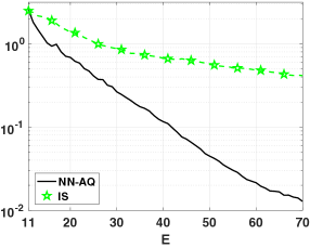
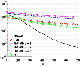
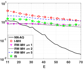
8.1.1 Experiment 1

We set $d_{x}=2$ and test the different algorithms in order to compute the vector mean $\bm{\mu}=[-0.4,0]$ and the diagonal of the covariance matrix $[\sigma_{1}^{2},\sigma_{2}^{2}]=[1.3813,8.9081]$. Moreover, our schemes are also able to estimate $Z$, whose ground-truth is $Z=7.9979$, thus we also measure the error in this estimation. We compare the performance in terms of Relative Mean Square Error (Rel-MSE), averaged over 500 independent runs, using different methodologies: (a) NN-AQ starting with $N_{0}=10$ nodes randomly chosen in $[-10,10]\times[-10,10]$ and $M=10^{5}$; (b) an independent MH algorithm (I-MH) with random initialization in $[-10,10]\times[-10,10]$; (c) random-walk MH algorithms (RW-MH) with different proposal variance, and random initialization in $[-10,10]\times[-10,10]$; (d) an IS algorithm. The proposal density for both I-MH and IS is a uniform in $[-10,10]\times[-10,10]$, whereas for the RW-MHs is a Gaussian density centered at the current state of the chain with covariance matrix $v^{2}{\bf I}$ where $v\in\{1,2,5\}$ (so we consider $3$ different RW-MHs).
For a fair comparison, we need that all methods have the same number $E$ of target evaluations (fixing $E=70$). Since NN-AQ, I-MH and RW-MH require one new target evaluation per iteration, we run $T=70$ iterations for I-MH and RW-MH ($E=T$), and $T-N_{0}=60$ iterations for NN-AQ. In this regard, the IS algorithm use 70 samples drawn from the uniform proposal. Hence, all methods need $T=70$ target evaluations. The results are given in Figures 3(a)-(b). Note that the estimation of $Z$ via MCMC techniques is not straightforward (e.g., see [71]).
Discussion 1. We can observe that NN-AQ outperforms the other methods in terms of Rel-MSE in estimation. Moreover, in Fig. 3(a)-(b) we can see that the decrease is much greater, as $E$ grows, than the other methods. Namely, NN-AQ has more benefits with new evaluations of $\pi({\bf x})$.

8.1.2 Experiment 2

In this case, we fix the number of target evaluations $E$, and vary $d_{x}=\{2,3,4,5\}$. The Rel-MSE in the estimation of $Z$ is given in Table 2 (with $E\in\{100,1000\}$).
Discussion 2. In this experiment, $E$ is fixed along different dimensions. The results given in Table 2, with fixed $E$, does not show all the potential of NN-AQ. However, NN-AQ outperforms IS in all the dimensions $d_{x}$ considered when $E=1000$.

Table 2: Relative MSE of $Z$ with $E\in\{100,1000\}$ for different $d_{x}$

methods	$E$	$d_{x}=2$	$d_{x}=3$	$d_{x}=4$	$d_{x}=5$
NN-AQ	100	0.0027	0.1127	0.3798	1.9730
	1000	4$\cdot 10^{-4}$	0.0023	0.0140	0.0374
IS	100	0.2645	0.4427	0.7627	1.1115
	1000	0.0226	0.0378	0.0641	0.1094

Figure 4: (a) Rel-MSE in log-scale for $Z$ as function of number of target evaluations $E$. (b) Rel-MSE in log-scale for $\bm{\mu}$ as function of number of target evaluations $E$. (b) Rel-MSE in log-scale for estimating $[\sigma_{1}^{2},\sigma_{2}^{2}]$ as function of number of target evaluations $E$.

Figure 5: (a) Example of application of GK-AQ with 10 starting points (red cross-marks) and T=60 iterations (red dots), i.e., $E=70$ target evaluations. (b) Rel-MSE in log-scale for $Z$ as function of number of target evaluations $E$. (c) Rel-MSE in log-scale for $\bm{\mu}$ as function of number of target evaluations $E$. (d) Rel-MSE in log-scale for estimating $[\sigma_{1}^{2},\sigma_{2}^{2}]$ as function of number of target evaluations $E$.

8.1.3 Experiment 3

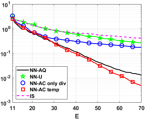
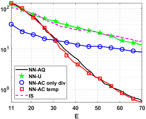
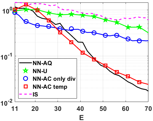
For $d_{x}=2$, we compare now IS, NN-AQ, and three variants of NN-AQ: (i) NN-U, where the optimization step in (31) is substituted with sampling uniformly the new node in $[-10,10]\times[-10,10]$ (i.e., without using an acquisition function), (ii) NN-AQ only diversity, which uses the acquisition in (35) with $\alpha=0$, $\beta=1$, i.e., with only the diversity term $D_{t}({\bf x})$, and (iii) NN-AQ tempered, which uses the acquisition in (35) with $\alpha=0$, $\beta_{t}=\frac{200}{t}$, i.e., $A_{t}({\bf x})=[D_{t}({\bf x})]^{\beta_{t}}$. Note that the adaptation in NN-AQ only diversity can be viewed as filling the space in a deterministic way. Note also that the adaptation in NN-AQ tempered will encourage more exploration than NN-AQ in the early iterations. Again, we compare the error in estimating $Z$, $\bm{\mu}$ and $[\sigma_{1}^{2},\sigma_{2}^{2}]$ as a function of target evaluations $E$ (up to $E=70$). The results are given in Figures 4(a)-(b).
Discussion 3. We can observe that NN-AQ and NN-AQ tempered outperform the others in terms of Rel-MSE in estimation. Moreover, in Fig. 4(a)-(b) we can see that for NN-AQ and NN-AQ tempered, the RMSE decreases at a faster rate as $E$ grows, than the NN-U and NN-AQ only diversity, highlighting the importance of taking into account the current interpolant to locate the new nodes. It can be seen that NN-AQ only diversity works much better than NN-U in the early iterations. We explain these results by the fact that NN-AQ only diversity tends to cover the space more efficiently in these early iterations since it avoids placing new nodes near the existing ones. However, as $E$ grows, the performance of NN-U and NN-AQ only diversity is similar since both end up filling uniformly the space. Interestingly, NN-U performs better than IS as $E$ increases, which demonstrate the power of the interpolative approach even when the new nodes are randomly chosen.

8.1.4 Experiment 4

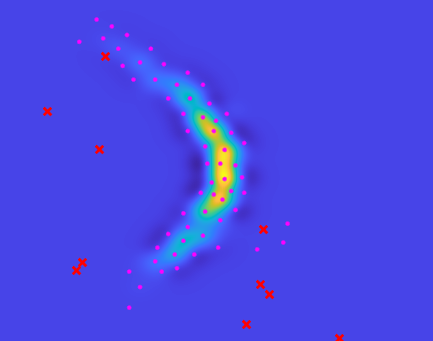
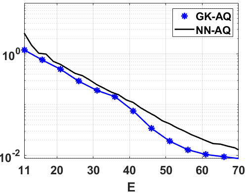
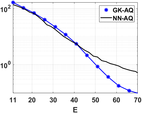
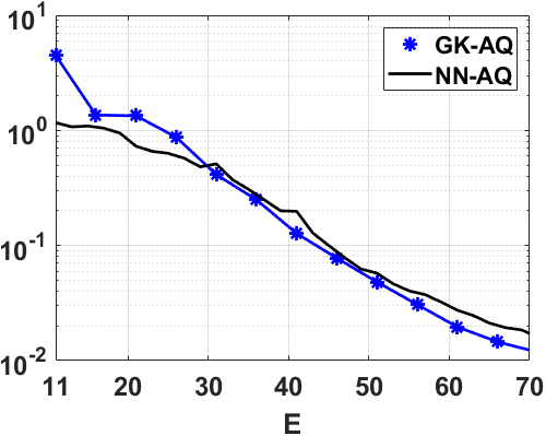
For $d_{x}=2$, we investigate the performance of GK-AQ in the estimation of $Z$, $\bm{\mu}$ and $[\sigma_{1}^{2},\sigma_{2}^{2}]$ as function of $E$. NN-GK employs the acquisition in (33). The kernel bandwidth $h$ is fitted using the procedure in Appendix A. As commented in Sect. 3.2, we consider a small noise of $\sigma=10^{-2}$ for numerical stability. We will compare the performance against NN-AQ. The results are given in Figures 5(a)-(d), along with an example of GK-AQ interpolant , with $E=70$, obtained in a specific run.

Discussion 4. The results are shown in Figures 5(b)-(d). GK-AQ outperforms NN-AQ in this particular experiment. However, it is important to remark that the results of GK-AQ may worsen considerably if $h$ is not selected adequately (we have used the procedure in App. A), in contrast to NN-AQ which is free of hyperparameter tuning and hence more robust.

8.2 Multimodal target

In this experiment, we consider a multimodal Gaussian target in $d_{x}=10$,

$$\bar{\pi}({\bf x})=\frac{1}{3}\mathcal{N}({\bf x}|\bm{\mu}_{1},{\bf\Sigma}_{1})+\frac{1}{3}\mathcal{N}({\bf x}|\bm{\mu}_{2},{\bf\Sigma}_{2})+\frac{1}{3}\mathcal{N}({\bf x}|\bm{\mu}_{3},{\bf\Sigma}_{3}),$$

with $\bm{\mu}_{1}=[5,0,\dots,0]$, $\bm{\mu}_{2}=[-7,0,\dots,0]$, $\bm{\mu}_{3}=[1,\dots,1]$ and ${\bf\Sigma}_{1}={\bf\Sigma}_{2}={\bf\Sigma}_{3}=4^{2}{\bf I}_{10}$. We want to test the performance of the different methods in estimating the normalizing constant $Z=1$. We consider an application of GK-AQ with $N_{0}=500$ initial nodes, random in $[-15,15]^{10}$, and $T=1000-N_{0}$, hence fixing the number of evaluations to $E=1000$. We compare it against three sophisticated AIS schemes, namely PMC, LAIS and AMIS [72]. For PMC, we choose Gaussian proposal pdfs and test different number of proposals $L\in\{10,100,200,500\}$, whose means are also initialized at random in $[-15,15]^{10}$. At each iteration one sample is drawn from each proposal, hence the algorithm is run for $T_{\text{PMC}}=\frac{1000}{L}$ iterations for a fair comparison. As a second alternative, we consider the deterministic mixture weighting approach for PMC, which is shown to have better overall performance, denoted DM-PMC. For LAIS, we also consider different number of proposals $L\in\{10,100,200,500\}$. More specifically, we consider two versions of LAIS: the one-chain version and an ideal version. In ideal LAIS, the means of the $L$ Gaussian proposals are drawn exactly from $\bar{\pi}({\bf x})$. The one-chain application of LAIS (OC-LAIS) requires to run a MCMC algorithm targeting $\bar{\pi}({\bf x})$ to obtain the $L$ proposal means, hence it requires $L$ evaluations of the target. At each iteration one sample is drawn from the mixture of the $L$ Gaussian proposals, hence we run the algorithm for $T_{\text{LAIS}}=1000-L$ iterations for a fair comparison. We used a Gaussian random walk Metropolis to obtain the $L$ means in the one-chain scenario. Finally, we consider AMIS with several combinations of number of iterations $T_{\text{AMIS}}$ and number of samples per iteration $R$. At each iteration, $R$ samples are drawn from a single Gaussian proposal, hence the total number of evaluations is $E=RT_{\text{AMIS}}$. In this case, we test $E\in\{1000,2000,3000,5000\}$, so the comparison is not fair except for $E=1000$. For PMC, LAIS and AMIS, as well as for the random walk proposal within the Metropolis algorithm, the covariance of the Gaussian proposals was fixed to $h^{2}{\bf I}_{10}$ (for $h=1,...,6$), where $h$ is the initial bandwidth parameter used in GK-AQ. All the methods are compared through the mean absolute error (MAE) in estimating $Z$, and the results are averaged over 500 independent simulations. The results are shown in Table 3 and Table 4. For each method, the best and worst MAE are boldfaced.
Discussion. We can observe that GK-AQ obtains the best range of MAE values $[0.078,0.4782]$ and the best results for $h=1$. For $h>1$, we can see in Tables 3-4 that the lowest MAE values are obtained by ideal LAIS with $L=500$ and $h=3$. We stress that ideal LAIS is not available in practice, since we usually cannot sample directly from $\bar{\pi}({\bf x})$. Regardless of the ideal LAIS scheme (not applicable in practice), GK-AQ provides the best results. Moreover, we see that GK-AQ with $h=3$ is the best performing method in this experiment, since it achieves a lower MAE than PMC, DM-PMC and OC-LAIS for every combination of $L$ and $h$. Table 4 shows that AMIS performs worse than GK-AQ for $E=1000$ (fair comparison), but even with much more AMIS evaluations $E\in\{2000,3000\}$ (unfair comparison in favor of AMIS). AMIS needs to reach a big enough value of $E$ ($E=5000$), to beat GK-AQ in terms of MAE.

Table 3: MAE of $Z$ with $E=1000$ (best and worst MAE of each method are boldfaced)

Methods		${\bf h=1}$	${\bf h=2}$	${\bf h=3}$	${\bf h=4}$	${\bf h=5}$	${\bf h=6}$
GK-AQ		0.4782	0.1741	0.0780	0.1362	0.1497	0.2322
PMC	$N=10$	0.9993	0.9526	0.8603	0.6743	0.6024	0.6155
	$N=100$	0.9998	0.9896	0.8853	0.6761	0.5192	0.4544
	$N=200$	1.0002	0.9893	0.8816	0.7099	0.6389	0.5384
	$N=500$	0.9995	0.9916	0.9741	0.8700	0.7421	0.6544
DM-PMC	$N=10$	0.9991	0.9478	0.8505	0.6009	0.5352	0.5814
	$N=100$	0.9997	0.8719	0.4490	0.2425	0.1901	0.2193
	$N=200$	0.9999	0.9321	0.5708	0.3257	0.2374	0.2524
	$N=500$	1.0000	0.9888	0.7969	0.5009	0.3684	0.3800
Ideal LAIS	$N=10$	0.9992	0.8114	0.2579	0.0863	0.0819	0.1091
	$N=100$	0.9918	0.3638	0.0547	0.0407	0.0598	0.1053
	$N=200$	0.9846	0.2486	0.0352	0.0411	0.0680	0.1093
	$N=500$	0.9687	0.1852	0.0335	0.0473	0.0891	0.1353
OC-LAIS	$N=10$	1.0000	1.0000	0.9992	0.9883	0.9468	0.9079
	$N=100$	0.9999	0.8731	0.4434	0.2785	0.2392	0.2870
	$N=200$	0.9982	0.7028	0.2418	0.1243	0.1406	0.2070
	$N=500$	0.9937	0.4949	0.1221	0.0857	0.1195	0.1786

Table 4: MAE of $Z$ of AMIS with $E\in\{1000,2000,3000,5000\}$

Methods		${\bf h=1}$	${\bf h=2}$	${\bf h=3}$	${\bf h=4}$	${\bf h=5}$	${\bf h=6}$
GK-AQ (E=1000)		0.4782	0.1741	0.0780	0.1362	0.1497	0.2322
AMIS	$M=10$	0.9998	0.9997	0.9997	0.9996	0.9996	0.9995
$E=1000$	$M=100$	1.0000	1.0000	1.0000	0.9999	0.9997	0.9990
	$M=200$	1.0000	1.0000	1.0000	1.0000	0.9998	0.9994
	$M=500$	1.0000	1.0000	1.0000	1.0000	0.9998	0.9989
AMIS	$M=10$	0.9155	0.9117	0.8981	0.8987	0.8891	0.8878
$E=2000$	$M=100$	0.9998	0.9986	0.9934	0.9784	0.9559	0.9072
	$M=200$	1.0000	1.0000	0.9998	0.9981	0.9888	0.9712
	$M=500$	1.0000	1.0000	1.0000	0.9998	0.9984	0.9953
AMIS	$M=10$	0.3293	0.3402	0.3051	0.3381	0.3540	0.3443
$E=3000$	$M=100$	0.9725	0.9040	0.7963	0.6384	0.4964	0.3816
	$M=200$	0.9998	0.9977	0.9884	0.9527	0.8308	0.7119
	$M=500$	1.0000	1.0000	0.9998	0.9988	0.9859	0.9566
AMIS	$M=10$	0.0766	0.0768	0.0695	0.0722	0.0699	0.0725
$E=5000$	$M=100$	0.1626	0.1176	0.0957	0.0810	0.0737	0.0656
	$M=200$	0.8771	0.6040	0.2824	0.1473	0.1163	0.0899
	$M=500$	1.0000	0.9982	0.9904	0.9449	0.7944	0.4532

8.3 Applications to exoplanet detection

In recent years, the problem of revealing objects orbiting other stars has acquired large attention. Different techniques have been proposed to discover exo-objects but, nowadays, the radial velocity technique is still the most used [73, 74, 75, 76]. The problem consists in fitting a dynamical model to data acquired at different moments spanning during long time periods (up to years). The model is highly non-linear and, for certain sets of parameters, its evaluation is quite costly in terms of computation time. This is due to the fact that its evaluation involves numerically integrating a differential equation, or using an iterative procedure for solving a non-linear equation (until a certain condition is satisfied). This loop can be very long for some sets of parameters.

Table 5: Description of parameters in Eq. (39).

Parameter	Description	Units
For each planet
$K_{i}$	amplitude of the curve	m s-1
${u}_{i,t}$	true anomaly	rad
$\omega_{i}$	longitude of periastron	rad
$e_{i}$	orbit’s eccentricity	…
$P_{i}$	orbital period	s
$\tau_{i}$	time of periastron passage	s
Below: not depending on the number of objects/satellite
$V_{0}$	mean radial velocity	m s-1

8.3.1 Likelihood function

When analyzing radial velocity data of an exoplanetary system, it is commonly accepted that the wobbling of the star around the center of mass is caused by the sum of the gravitational force of each planet independently and that they do not interact with each other. Each planet follows a Keplerian orbit and the radial velocity of the host star is given by

$${y}_{t}=V_{0}+\sum\limits_{i=1}^{S}K_{i}\left[\cos\left({u}_{i,t}+\omega_{i}\right)+e_{i}\cos\left(\omega_{i}\right)\right]+\xi_{t},$$ (39)

with $t=1,\ldots,T$. The number of objects in the system is $S$. Both ${y}_{t}$, ${u}_{i,t}$ depend on time $t$, and $\xi_{t}$ is a Gaussian noise perturbation with variance $\sigma_{e}^{2}$. We consider the noise variance $\sigma_{e}^{2}$ an unknown parameter as well. The meaning of each parameter in Eq. (39) is given in Table 5. The likelihood function is jointly defined by (39) and some indicator variables described below. The angle ${u}_{i,t}$ is the true anomaly of the planet $i$ and it can be determined from

$$\frac{d{u}_{i,t}}{dt}=\frac{2\pi}{P_{i}}\frac{\left(1+e_{i}\cos{u_{i,t}}\right)^{2}}{\left(1-e_{i}\right)^{\frac{3}{2}}}$$

This equation has an analytical solution. As a result, the true anomaly $u_{i,t}$ can be determined from the mean anomaly $M_{i,t}$. However, the analytical solution contains a non-linear term that needs to be determined by iterating. First, we define the mean anomaly $M_{i,t}$ as

$$M_{i,t}=\frac{2\pi}{P_{i}}\left(t-\tau_{i}\right),$$

where $\tau_{i}$ is the time of periastron passage of the planet $i$ and $P_{i}$ is the period of its orbit (see Table 5). Then, through the Kepler’s equation,

$$M_{i,t}=E_{i,t}-e_{i}\sin E_{i,t},$$ (40)

where $E_{i,t}$ is the eccentric anomaly. Equation (40) has no analytic solution and it must be solved by an iterative procedure. A Newton-Raphson method is typically used to find the roots of this equation [77]. For certain sets of parameters, this iterative procedure can be particularly slow and the computation of the likelihood becomes quite costly. We also have

$$\tan\frac{u_{i,t}}{2}=\sqrt{\frac{1+e_{i}}{1-e_{i}}}\,\tan\frac{E_{i,t}}{2},$$ (41)

Therefore, the variable of interest $\mathbf{x}$ is the vector of dimension $d_{X}=1+5S$ (where $S$ is the number of planets),

$$\mathbf{x}=[V_{0},K_{1},\omega_{1},e_{1},P_{1},\tau_{1},\ldots,K_{S},\omega_{S},e_{S},P_{S},\tau_{S}],$$

For a single object (e.g., a planet or a natural satellite), the dimension of $\mathbf{x}$ is $d_{X}=5+1=6$, with two objects the dimension of $\mathbf{x}$ is $d_{X}=11$, etc. All the Eqs. from (39) to (41) induce a likelihood function $\ell({\bf y}|\mathbf{x},\sigma_{e})=\prod_{t=1}^{T}\ell(y_{t}|\mathbf{x},\sigma_{e})$, where ${\bf y}=\{y_{1},\ldots,y_{T}\}$.

8.3.2 Prior and posterior densities

The prior $g({\bf x})$ is defined as multiplication of indicator variables $V_{0}\in[-20,20]$, $K_{i}\in[0,\max y_{i,t}-\min y_{i,t}]$, $e_{i}\in[0,1]$, $P_{i}\in[0,365]$, $\omega_{i,t}\in[0,2\pi]$, $\tau_{i}\in[0,30]$, (i.e., the prior is zero outside these intervals), for all $i=1,\ldots,S$. This means that the prior density is zero when the particles fall out of these intervals. Note that the interval of $\tau_{i}$ is conditioned to the value $P_{i}$. This parameter is the time of periastron passage, i.e. the time passed since the object crossed the closest point in its orbit. It has the same units of $P_{i}$ and can take values from 0 to $P_{i}$. The complete posterior is

$$p(\mathbf{x}|{\bf y},\sigma_{e})=\frac{1}{p({\bf y}|\sigma_{e})}\ell({\bf y}|\mathbf{x},\sigma_{e})g({\bf x}).$$

We are interested in inferring the parameters ${\bf x}$ and, more specifically, computing the marginal likelihood

$$Z=p({\bf y}|\sigma_{e})=\int_{\mathcal{X}}\ell({\bf y}|\mathbf{x},\sigma_{e})g({\bf x})d{\bf x},$$

obtained integrating out ${\bf x}$, in order to infer the number of planets. The noise variance $\sigma_{e}^{2}$ is also inferred after the sampling, by maximizing $Z=p({\bf y}|\sigma_{e})$, i.e., $\widehat{\sigma}_{e}^{2}=\arg\max\limits_{\sigma_{e}}p({\bf y}|\sigma_{e})$.

8.3.3 Experiments

Given a set of data ${\bf y}$ generated according to the model (see the initial parameter values below), our goal is to infer the number $S$ of planets in the system. For this purpose, we have to approximate the model evidence $Z=p({\bf y}|\sigma_{e})$ of each model. In all experiments, we consider $60$ total number of observations. We consider three different experiments: (E1) $S=0$, i.e., no object, (E2) $S=1$ (one object) and (E2) the case of two objects $S=2$. We set $V=2$, in all cases. For the first object in E1 and E2, we set $K_{1}=25$, $\omega_{1}=0.61$, $e_{1}=0.1$, $P_{1}=15$, $\tau_{1}=3$. For E2, we also consider a second object with $K_{2}=5$, $\omega_{2}=0.17$, $e_{2}=0.3$, $P_{2}=115$, $\tau_{2}=25$ (in that case $S=2$). All the data are generated with $\sigma_{e}^{2}=2$. The rest of trajectories are generated according to the transition model (and the corresponding measurements $y_{t}$ according to the observation model).

8.3.4 Methods

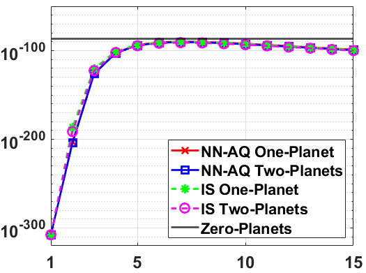
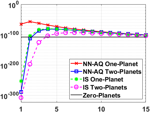
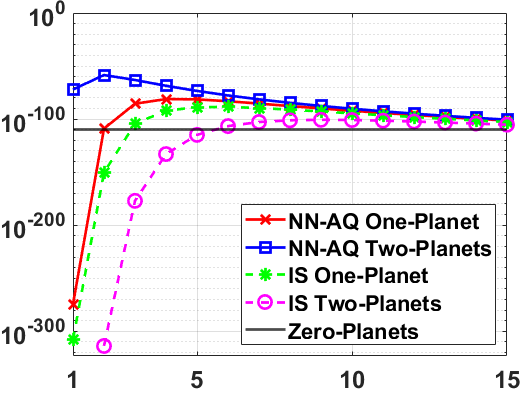
For each experiment, three models (i.e. three different target pdfs) are considered: a model with $S=0$ (Zero-Planets), a model with $S=1$ (One-Planet) and a model with $S=2$ (Two-Planets). The goal is to estimate the marginal likelihood of these models and then correctly detect the number of planets, i.e., $S=0$ for (E1), $S=1$ for (E2) and $S=2$ for (E3). The marginal likelihoods corresponding to the Zero-planets models are available in closed form and need not be estimated (the model is simply Gaussian in that case). For this purpose, we apply NN-AQ (with $M=10^{7}$) and and an IS procedure. We allocate a budget of $4\cdot 10^{6}$ evaluations of the target. In IS, this budget is used to draw $4\cdot 10^{6}$ samples from the priors. While NN-AQ uses first $4\cdot 10^{6}-5000$ of these samples to look for a good initialization, more specifically, the sample with the highest target evaluation is kept, along with 9 more samples taken at random, to use them as initial nodes. Then, NN-AQ is run for $5000$ iterations. Both One-Planet and Two-Planets models are estimated for different values of $\sigma_{e}=1,2,\dots,15$. Note that we do not need to evaluate the target again when considering different $\sigma_{e}$, i.e., a single target evaluation can be reused for all values of $\sigma_{e}$. The results are shown in Figure 6.

(a) Zero planets

(b) One planet

(c) Two planets

Figure 6: Plot of marginal likelihood estimates of Model 1 (one-planet) and Model 2 (two-planets) versus $\sigma$ for the three data sets. The straight lines represent the known marginal likelihoods of Model 0 (zero planets) for each data set. (a) data set with zero planets, (b) data set with one planet, (c) data set with two planets.

8.3.5 Results

For each experiment (E1)-(E3), Figure 6(a)-(c) depicts the estimations of $Z$ of the different models provided by NN-AQ and IS, versus $\sigma_{e}$. The horizontal lines correspond to the known marginal likelihoods of Zero-Planets models. Overall, NN-AQ outperforms IS and predicts correctly the number of planets as well as the true value of $\sigma_{e}$ (indeed, the curves corresponding to NN-AQ reach a maximum at $\sigma_{e}=2$). Figure 6(a) shows that the estimations provided by NN-AQ and IS correctly rank the Zero-planets model ($S=0$) as the most probable one. Figure 6(b) shows both NN-AQ and IS predict correctly the One-Planet model ($S=1$) to be the correct one. However, for $\sigma_{e}=2$, IS barely differentiates between the Zero-Planet and One-Planets models. Further, for $\sigma_{e}=1$, it wrongly predicts Zero-Planets as the best one. Conversely, NN-AQ is able to predict the correct model for every value of $\sigma_{e}$, and besides, also predicts the true value $\sigma_{e}=2$. In Figure 6(c), the difference in performance of NN-AQ and IS is more acute. While NN-AQ is able to correctly predict the Two-Planets model ($S=2$) as the most probable for all values of $\sigma_{e}$, IS is unable to detect that second planet and, therefore, considers the One-Planet model more probable. As in the previous case, IS fails at detecting any planet for small values of $\sigma_{e}$. Again, NN-AQ predict the correct value of $\sigma_{e}$.

9 Conclusions

In this work, we have described a general framework for adaptive interpolative quadrature schemes, leveraging an in-depth study of different fields and related techniques in the literature, such as Bayesian quadrature algorithms, scattered data approximations, emulation, experimental design and active learning schemes. The nodes of the quadrature are adaptively chosen by maximizing a suitable acquisition function, which depends on the current interpolant and the positions of the nodes. This maximization does not require extra evaluations of the true posterior. The proposed methods supply also a surrogate model (emulator) which approximates the true posterior density, that can be also employed in further statistical analyses. Two specific schemes, based on Gaussian and NN bases, have been described. In both cases, a non-negative estimation $\widehat{Z}$ of the marginal likelihood $Z$ is ensured.
In the proposed framework, we also relax the assumptions regarding the kernel-basis functions with respect to other approaches in the literature, e.g., the bases could be non-symmetric. For instance, the NN bases are non-symmetric functions and their use has different important benefits: (a) they ensure obtaining non-negative interpolation coefficients and estimators $\widehat{Z}$, (b) the linear system is directly solved without the need of inverting any matrix (the interpolation matrix is always diagonal), and (c) the bandwidth of the bases are automatically selected. Our scheme also allows selecting different kernel functions for each node point. Therefore, the quadrature rules in Bayesian quadrature are a special case of our proposed scheme. Indeed, Bayesian quadrature considers a single symmetric and semi positive definite kernel function. An importance sampling interpretation has been also provided. It is important to remark that the true posterior is only evaluated at the nodes selected sequentially by the algorithm, and the rest of other computations does not query the true model. The convergence of the proposed quadrature rules has been discussed, jointly with other theoretical results. The new algorithms are powerful techniques as also shown by several numerical experiments.

Figure 7: (a) GK based interpolant with $N_{T}=70$ nodes and $h=2.7$, fitted by maximizing the marginal likelihood. (b) Plot of $\widehat{Z}$ as function of $h$. The value of $h$ at which $\widehat{Z}$ attains the local maximum is used to build the interpolant in our procedure. (d) GK based interpolant with $N_{T}=70$ nodes and $h=0.51$ fitted with the heuristic.

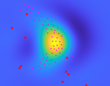
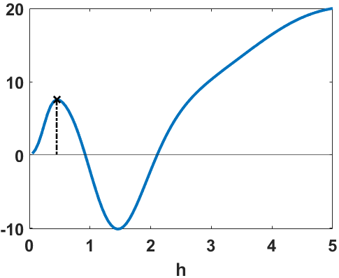
Appendix A Procedure for tuning the Gaussian kernel bandwidth

In this Appendix, we propose a procedure for fitting the bandwidth parameter $h$ of the Gaussian kernel (GK),

$$k_{G}({\bf x},{\bf x}_{i})=\frac{1}{(2\pi)^{\frac{d_{x}}{2}}h^{d_{x}}}\exp\left(-\frac{1}{2h^{2}}({\bf x}-{\bf x}_{i})^{\top}({\bf x}-{\bf x}_{i})\right),$$ (42)

when building the GK based interpolant of Sect. 3 for a given number of nodes. Assume we have run the GK-AQ algorithm (with some fixed $h_{0}$), so we have a total of $N_{T}$ nodes. Now, for any $h$, we may solve the linear system (Eq. (5)), obtain the coefficients $\{\beta_{i}\}_{i=1}^{N_{T}}$ and calculate

$$\widehat{Z}=\sum_{i=1}^{N_{T}}\beta_{i}.$$ (43)

Note that, although not explicit, the $\beta_{i}$’s, and hence $\widehat{Z}$, depend on $h$. The proposed procedure consists of taking $h$ as the value where $\widehat{Z}$ attains its first local maximum. Starting from a small value $h$ close to zero and increasing it, the estimation $\widehat{Z}$ is growing reaching a maximum. Then, $h$ is starting to become “too big”, producing too much overlapping among the kernel areas. The values of the elements out the diagonal of ${\bf K}$ grow, and some of the coefficients $\beta_{i}$ are negative, and the estimation $\widehat{Z}$ decreases. As $h$ becomes greater and greater, the matrix ${\bf K}$ tends to become ill-conditioned, and the absolute values of $\beta_{i}$’s grows. Figure 7 compares the GK based interpolant of the target from Sect 8.1 with two different choices of $h$ and $N_{T}=70$ nodes. Figure 7(a) plots the interpolant taking $h$ as the value which minimizes the marginal likelihood (see Sect. 3.2). Note that this value of $h$ is too big given the dispersion of the nodes. While Figure 7(c) plots the interpolant taking $h$ as the value where the curve of $\widehat{Z}$ (Figure 7(b)) attains its local maximum. This choice of $h$ seems to fit better the existing nodes. Note also that, for some values of $h$, $\widehat{Z}$ may be negative.

Appendix B Probabilistic interpretation of $J$

Let us consider $J=\int_{\mathcal{X}}f({\bf x})\pi({\bf x})d{\bf x}$, which is the numerator of (1), our integral of interest $I$. In section 3.1, we have seen that, when $k({\bf x},{\bf x}_{i})=k({\bf x}_{i},{\bf x})$ (i.e., a symmetric basis function), the interpolant $\widehat{\pi}({\bf x})=\sum_{i=1}^{N}\beta_{i}k({\bf x},{\bf x}_{i})$ has the probabilistic interpretation of being the mean of the posterior distribution of (the “unknown”) $\pi({\bf x})$ after observing ${\bf d}=[\pi({\bf x}_{1}),\dots,\pi({\bf x}_{N})]^{\top}$, i.e., $\mathbb{E}[\pi({\bf x})|{\bf d}]=\widehat{\pi}({\bf x})$. The distribution on $\pi({\bf x})$ induces a posterior distribution on $J$, which is a Gaussian with mean

$$\mathbb{E}[J|{\bf d}]=\widetilde{J}=\int_{\mathcal{X}}f({\bf x})\widehat{\pi}({\bf x})d{\bf x},$$ (44)

and variance given by

$$\text{var}[J|{\bf d}]=\int\int k({\bf x},{\bf x}^{\prime})f({\bf x})f({\bf x}^{\prime})d{\bf x}d{\bf x}^{\prime}-\bm{\zeta}^{\top}{\bf K}^{-1}\bm{\zeta},$$ (45)

where $\bm{\zeta}=[J_{1},\dots,J_{N}]$ and $J_{i}=\int_{\mathcal{X}}f({\bf x})k({\bf x},{\bf x}_{i})d{\bf x}$. This interpretation corresponds to the so-called Bayesian quadrature, which uses Eq. (44) as approximation of $J$. Note that Eq. (44) is the quadrature obtained by substituting the true $\pi({\bf x})$ with its interpolant $\widehat{\pi}({\bf x})$, which coincides with the numerator of $\widehat{I}$ in Eq. (7).

Appendix C Recursive inversion of a bordered matrix

The most costly step when calculating $\bm{\beta}$ in (5) consists in inverting the $N\times N$ matrix $({\bf K})_{i,j}=k({\bf x}_{i},{\bf x}_{j})$ ($i,j\in\{1,\dots,N\}$). Moreover, every time a new node is added, the $\beta_{i}$ must be recomputed, so the step of computing the inverse has to be done again. This time the matrix is bigger due to adding a new node, that is, it has an additional row and column. We show that knowing ${\bf K}^{-1}$ help us to compute the inverse of augmented matrices (called “bordered matrix”, i.e., adding a “border” of new row and column to an existing matrix).
Let us denote with ${\bf K}_{N}$ the matrix built using $N$ nodes, and let ${\bf K}_{N+1}$ be the matrix with $N+1$ nodes. Of course we have

$${\bf K}_{N+1}=\begin{pmatrix}{\bf K}_{N}&{\bf k}_{N}\\ {\bf k}^{T}_{N}&k\end{pmatrix}$$ (46)

where ${\bf k}_{N}=(k({\bf x}_{1},{\bf x}_{N+1}),k({\bf x}_{2},{\bf x}_{N+1}),\dots,k({\bf x}_{N},{\bf x}_{N+1}))^{T}$ and $k=k({\bf x}_{N+1},{\bf x}_{N+1})$. The $(N+1)\times(N+1)$ inverse of ${\bf K}_{N+1}$ can be expressed in terms of ${\bf K}^{-1}_{N}$ as follows

$${\bf K}_{N+1}^{-1}=\begin{pmatrix}{\bf A}&{\bf b}\\ {\bf c}&s\end{pmatrix},$$ (47)

where

$${\bf A} ={\bf K}^{-1}_{N}+{\bf K}_{N}^{-1}{\bf k}_{N}\left(k-{\bf k}_{N}^{T}{\bf K}_{N}^{-1}{\bf k}_{N}\right)^{-1}{\bf k}_{N}^{T}{\bf K}_{N}^{-1}\in\mathbb{R}^{N\times N},$$

$${\bf b} =-{\bf K}^{-1}_{N}{\bf k}_{N}\left(k-{\bf k}^{T}_{N}{\bf K}^{-1}_{N}{\bf k}_{N}\right)^{-1}\in\mathbb{R}^{N\times 1},$$

$${\bf c} =-\left(k-{\bf k}^{T}_{N}{\bf K}^{-1}_{N}{\bf k}_{N}\right)^{-1}{\bf k}^{T}_{N}{\bf K}^{-1}_{N}\in\mathbb{R}^{1\times N},$$

$$s =\left(k-{\bf k}_{N}^{T}{\bf K}_{N}^{-1}{\bf k}_{N}\right)^{-1}\in\mathbb{R}.$$

Note that computing $s=\left(k-{\bf k}_{N}^{T}{\bf K}_{N}^{-1}{\bf k}_{N}\right)^{-1}$ is not costly since it is an scalar value.

Appendix D Proofs

D.1 Proof to theorem 1

We have that

$$|J-\widehat{J}| =\left|\int_{\mathcal{X}}f({\bf x})\pi({\bf x})d{\bf x}-\int_{\mathcal{X}}f({\bf x})\widehat{\pi}({\bf x})d{\bf x}\right|$$

$$=\left|\int_{\mathcal{X}}f({\bf x})\left(\pi({\bf x})-\widehat{\pi}({\bf x})\right)d{\bf x}\right|.$$

It is easy to see that, for any $g({\bf x})$ we have $-|g({\bf x})|\leq g({\bf x})\leq|g({\bf x})|$ for all ${\bf x}$, and that $-\int|g({\bf x})|d{\bf x}\leq\int g({\bf x})d{\bf x}\leq\int|g({\bf x})|d{\bf x}$, so we have $\left|\int g({\bf x})d{\bf x}\right|\leq\int|g({\bf x})|d{\bf x}$. Using this result we can state the first inequality

$$|J-\widehat{J}| =\left|\int_{\mathcal{X}}f({\bf x})\left(\pi({\bf x})-\widehat{\pi}({\bf x})\right)d{\bf x}\right|$$

$$\leq\int_{\mathcal{X}}\left|f({\bf x})\right|\left|\pi({\bf x})-\widehat{\pi}({\bf x})\right|d{\bf x}$$

$$=\left\lVert f(\pi-\widehat{\pi})\right\rVert_{1}.$$

The second inequality of the theorem follows from Holder’s inequality

$$\left\lVert f(\pi-\widehat{\pi})\right\rVert_{1}\leq\left\lVert f\right\rVert_{2}\left\lVert\pi-\widehat{\pi}\right\rVert_{2}.$$

Finally, the last inequality of the theorem is obtained after manipulating the $\left\lVert f\right\rVert_{2}$ and $\left\lVert\pi-\widehat{\pi}\right\rVert_{2}$,

$$\left\lVert f\right\rVert_{2}\left\lVert\pi-\widehat{\pi}\right\rVert_{2} =\left(\int_{\mathcal{X}}|f({\bf x})|^{2}d{\bf x}\right)^{\frac{1}{2}}\left(\int_{\mathcal{X}}|\pi({\bf x})-\widehat{\pi}({\bf x})|^{2}d{\bf x}\right)^{\frac{1}{2}}$$

$$\leq\left(|\mathcal{X}|\max|f({\bf x})|^{2}\right)^{\frac{1}{2}}\left(|\mathcal{X}|\max|\pi({\bf x})-\widehat{\pi}({\bf x})|^{2}\right)^{\frac{1}{2}}$$

$$=|\mathcal{X}|\max|f({\bf x})|\max|\pi({\bf x})-\widehat{\pi}({\bf x})|$$

$$=|\mathcal{X}|\left\lVert f\right\rVert_{\infty}\left\lVert\pi-\widehat{\pi}\right\rVert_{\infty}.$$

D.2 Proof to theorem 2

We provide the main concepts and elements of the proof. For more details, see [67, 16]. Let $J=\int_{\mathcal{X}}f({\bf x})\pi({\bf x})d{\bf x}$ and $\widetilde{J}=\sum_{i=1}^{N}\nu_{i}\pi({\bf x}_{i})$ be the integral of interest and the quadrature using points $\{{\bf x}_{i}\}_{i=1}^{N}$, respectively. Recall that we also denote $\bm{\nu}=[\nu_{1},\dots,\nu_{N}]^{\top}$.
Consider that $\pi$ is a function belonging to the reproducing kernel Hilbert space of functions $\mathcal{H}$ originated from the symmetric and positive definite kernel function $k({\bf x},{\bf x}^{\prime})$. Hence, $J$ and $\widetilde{J}$ are functionals over that RKHS

$$J[\pi] =\int_{\mathcal{X}}f({\bf x})\pi({\bf x})d{\bf x},$$

$$\widetilde{J}[\pi] =\sum_{i=1}^{N}\nu_{i}\pi({\bf x}_{i}),\enskip\pi\in\mathcal{H}.$$

where we write explicitly $J[\cdot]$ is the functional that integrates w.r.t. $f({\bf x})$, while $\widetilde{J}[\cdot]$ is the functional that integrates w.r.t. the weighted sum $\sum_{i=1}^{N}\nu_{i}\delta_{{\bf x}_{i}}$, where $\delta_{{\bf x}_{i}}$ denotes the point evaluation in ${\bf x}_{i}$. The integration error associated with $\widetilde{J}$ is characterized by the norm, in the dual space $\mathcal{H}^{*}$, of the error functional

$$\left\lVert J-\widetilde{J}\right\rVert_{\mathcal{H}^{*}}=\sup_{\left\lVert\pi\right\rVert_{\mathcal{H}}\leq 1}\left|\widetilde{J}[\pi]-J[\pi]\right|,$$ (48)

where $\left\lVert\cdot\right\rVert_{\mathcal{H}}$ and $\left\lVert\cdot\right\rVert_{\mathcal{H}^{*}}$ denote the norm in $\mathcal{H}$ and $\mathcal{H}^{*}$ respectively. Eq. (48) is also called worst-case error (WCE). Define the functions

$$k_{f}({\bf x})=\int_{\mathcal{X}}f({\bf x}^{\prime})k({\bf x},{\bf x}^{\prime})d{\bf x}^{\prime},$$ (49)

and

$$k_{\widetilde{f}}({\bf x})=\sum_{i=1}^{N}\nu_{i}k({\bf x},{\bf x}_{i}),$$ (50)

where $k_{f}$, $k_{\widetilde{f}}\in\mathcal{H}$. These functions exist as consequence of $\int_{\mathcal{X}}k({\bf x},{\bf x})f({\bf x})d{\bf x}<\infty$. It can be shown that $\left\lVert J-\widetilde{J}\right\rVert_{\mathcal{H}^{*}}=\left\lVert k_{f}-k_{\widetilde{f}}\right\rVert_{\mathcal{H}}$, and

$$\left\lVert J-\widetilde{J}\right\rVert^{2}_{\mathcal{H}^{*}} =\bm{\nu}^{\top}{\bf K}\bm{\nu}-2\bm{\nu}^{\top}\bm{\zeta}+\int_{\mathcal{X}}\int_{\mathcal{X}}f({\bf x})f({\bf x}^{\prime})k({\bf x},{\bf x}^{\prime})d{\bf x}d{\bf x}^{\prime},$$ (51)

for a vector of weights $\bm{\nu}\in\mathbb{R}^{N}$, the matrix $({\bf K})_{1\leq i,j\leq N}=k({\bf x}_{i},{\bf x}_{j})$, and the vector of integrals $\bm{\zeta}=[k_{f}({\bf x}_{1}),\dots,k_{f}({\bf x}_{N})]^{\top}$. Conditional on the fixed states $\{{\bf x}_{i}\}_{i=1}^{N}$, the weights $\bm{\nu}$ that minimizes the above expression are given by $\bm{\nu}={\bf K}^{-1}\bm{\zeta}$. These are the weights that arises if we build the interpolant $\widehat{\pi}$ of $\pi$ at points $\{{\bf x}_{i}\}_{i=1}^{N}$, using $k({\bf x},{\bf x}^{\prime})$ as the basis function, and substitute it in $J$ to obtain the quadrature.

D.3 Proof to theorem 6

Let $J$ be the integral of interest, and let $\tilde{J}=\sum_{i=1}^{N}\beta_{i}J_{i}$ and $\widehat{J}=\sum_{i=1}^{N}\beta_{i}\widehat{J}_{i}$ be the approximations using, respectively, the exact $J_{i}$ and the noisy estimation $\widehat{J}_{i}$ . Recall that the coefficients $\beta_{i}$ are written in matrix form as $\bm{\beta}={\bf K}^{-1}{\bf d}$ where ${\bf K}$ is the interpolation matrix and ${\bf d}$ is the vector of evaluations of $\pi$. Let us denote $\bm{\zeta}=[J_{1},\dots,J_{N}]^{\top}$ and $\widehat{\bm{\zeta}}=[\widehat{J}_{1},\dots,\widehat{J}_{N}]^{\top}$. Denoting the dot product in $\mathbb{R}^{N}$ as $\langle\cdot,\cdot\rangle$, we can express $\widetilde{J}=\langle\bm{\zeta},\bm{\beta}\rangle$ and $\widehat{J}=\langle\widehat{\bm{\zeta}},\bm{\beta}\rangle$. Thus

$$|J-\widehat{J}| =|J-\langle\widehat{\bm{\zeta}},\bm{\beta}\rangle|$$

$$=|J-\langle\bm{\zeta}-\bm{\zeta}+\widehat{\bm{\zeta}},\bm{\beta}\rangle|$$

$$=|J-\langle\bm{\zeta},\bm{\beta}\rangle+\langle\bm{\zeta},\bm{\beta}\rangle-\langle\widehat{\bm{\zeta}},\bm{\beta}\rangle|$$

$$\leq|J-\widetilde{J}|+|\langle\bm{\zeta}-\widehat{\bm{\zeta}},\bm{\beta}\rangle|$$

$$=|J-\widetilde{J}|+|\langle{\bf K}^{-1}(\bm{\zeta}-\widehat{\bm{\zeta}}),\bm{d}\rangle|$$

$$\leq||f(\pi-\widehat{\pi})||_{1}+||{\bf K}^{-1}(\bm{\zeta}-\widetilde{\bm{\zeta}})||_{2}\left\lVert{\bf d}\right\rVert_{2}$$

$$\leq|\mathcal{X}|\left||f|\right|_{\infty}||\pi-\widehat{\pi}||_{\infty}+||{\bf K}^{-1}||_{2}||\bm{\zeta}-\widehat{\bm{\zeta}}||_{2}\left||{\bf d}|\right|_{2}$$

where the norm $||{\bf K}^{-1}||_{2}$ represents the largest singular value of ${\bf K}^{-1}$. The bounds $\left\lVert\pi-\widehat{\pi}\right\rVert_{\infty}=\lambda(r)$ and $||{\bf K}^{-1}||_{2}=\mathcal{O}(\upsilon(s,h))$ for different RBF can be found respectively in Chapters 11.3 and 12.2 of [55]. For further details, see Proposition 1 in [67].

D.4 Proof to theorem 8

Let us consider the target $\pi({\bf x})$ and the interpolant $\widehat{\pi}({\bf x})$ based on NN constant kernels. Note that for all ${\bf x}\in\mathcal{X}$ we have $\widehat{\pi}({\bf x})=\pi({\bf x}^{*})$, where ${\bf x}^{*}=\arg\min_{i}\left\lVert{\bf x}-{\bf x}_{i}\right\rVert$, i.e., the node that is closest to ${\bf x}$. Lipschitz continuity implies that $|\pi({\bf z})-\pi({\bf x})|\leq L_{0}\left\lVert{\bf z}-{\bf x}\right\rVert$ for all ${\bf z},{\bf x}\in\mathcal{X}$. Hence,

$$\left\lVert\pi-\widehat{\pi}\right\rVert_{\infty} =\max_{{\bf x}\in\mathcal{X}}|\pi({\bf x})-\widehat{\pi}({\bf x})|$$

$$=\max_{{\bf x}\in\mathcal{X}}|\pi({\bf x})-\pi({\bf x}^{*})|$$

$$\leq L_{0}\max_{{\bf x}\in\mathcal{X}}\left\lVert{\bf x}-{\bf x}^{*}\right\rVert$$

$$=L_{0}\max_{{\bf x}\in\mathcal{X}}\min_{i}\left\lVert{\bf x}-{\bf x}_{i}\right\rVert$$

$$=L_{0}r,$$

where we used the definition of fill distance $r$, i.e.,

$$r=\max_{{\bf x}\in\mathcal{X}}\min_{i}\left\lVert{\bf x}-{\bf x}_{i}\right\rVert.$$

For further details, see [27, 56].

References

- Burden and Faires [2000] R. L. Burden and J. D. Faires, Numerical Analysis. Brooks Cole, 2000.
- Robert and Casella [2004] C. P. Robert and G. Casella, Monte Carlo Statistical Methods. Springer, 2004.
- Niederreiter [1992a] H. Niederreiter, Random Number Generation and Quasi-Monte Carlo Methods. Society for Industrial Mathematics, 1992.
- Martino et al. [2018a] L. Martino, D. Luengo, and J. Míguez, “Independent random sampling methods,” Springer, 2018.
- Liu and Pierce [1994] Q. Liu and D. A. Pierce, “A note on Gauss–Hermite quadrature,” Biometrika, vol. 81, no. 3, pp. 624–629, 1994.
- Jäckel [2005] P. Jäckel, “A note on multivariate Gauss–Hermite quadrature,” London: ABN-Amro. Re, 2005.
- Owen [2013] A. Owen, Monte Carlo theory, methods and examples, 2013.
- Elvira et al. [2020a] V. Elvira, L. Martino, and P. Closas, “Importance Gaussian quadrature,” arXiv:2001.03090, pp. 1–13, 2020.
- Akyildiz and Míguez [2020] O. D. Akyildiz and J. Míguez, “Nudging the particle filter,” Statistics and Computing, vol. 30, pp. 305–330, 2020.
- Liu and Lee [2017] Q. Liu and J. D. Lee, “Black-box importance sampling,” in Artificial Intelligence and Statistics (AISTATS), 2017.
- O’Hagan [1991] A. O’Hagan, “Bayes–Hermite quadrature,” Journal of statistical planning and inference, vol. 29, no. 3, pp. 245–260, 1991.
- Kennedy [1998] M. Kennedy, “Bayesian quadrature with non-normal approximating functions,” Statistics and Computing, vol. 8, no. 4, pp. 365–375, 1998.
- Rasmussen and Ghahramani [2003] C. E. Rasmussen and Z. Ghahramani, “Bayesian Monte Carlo,” Advances in neural information processing systems, pp. 505–512, 2003.
- Osborne et al. [2012] M. Osborne, R. Garnett, Z. Ghahramani, D. K. Duvenaud, S. J. Roberts, and C. E. Rasmussen, “Active learning of model evidence using Bayesian quadrature,” in Advances in neural information processing systems, 2012, pp. 46–54.
- Gunter et al. [2014] T. Gunter, M. A. Osborne, R. Garnett, P. Hennig, and S. J. Roberts, “Sampling for inference in probabilistic models with fast Bayesian quadrature,” in Advances in neural information processing systems, 2014, pp. 2789–2797.
- Briol et al. [2019] F.-X. Briol, C. J. Oates, M. Girolami, M. A. Osborne, and D. Sejdinovic, “Probabilistic integration: A role in statistical computation?” Statistical Science, vol. 34, no. 1, pp. 1–22, 2019.
- Karvonen and Särkkä [2017] T. Karvonen and S. Särkkä, “Classical quadrature rules via Gaussian processes,” in 2017 IEEE 27th International Workshop on Machine Learning for Signal Processing (MLSP). IEEE, 2017, pp. 1–6.
- Kanagawa and Hennig [2019] M. Kanagawa and P. Hennig, “Convergence Guarantees for Adaptive Bayesian Quadrature Methods,” in Advances in Neural Information Processing Systems, 2019, pp. 6234–6245.
- Busby [2009] D. Busby, “Hierarchical adaptive experimental design for Gaussian process emulators,” Reliability Engineering & System Safety, vol. 94, no. 7, pp. 1183–1193, 2009.
- Pratola et al. [2018] M. T. Pratola, C. D. Lin, and P. F. Craigmile, “Optimal design emulators: A point process approach,” arXiv preprint arXiv:1804.02089, 2018.
- Svendsen et al. [2020] D. H. Svendsen, L. Martino, and G. Camps-Valls, “Active emulation of computer codes with gaussian processes - application to remote sensing,” Pattern Recognition, vol. 100, p. 107103, 2020.
- Ying et al. [2020] H. Ying, K. Mao, and K. Mosegaard, “Moving Target Monte Carlo,” arXiv preprint arXiv:2003.04873, 2020.
- Rasmussen et al. [2003] C. E. Rasmussen, J. Bernardo, M. Bayarri, J. Berger, A. Dawid, D. Heckerman, A. Smith, and M. West, “Gaussian processes to speed up hybrid Monte Carlo for expensive Bayesian integrals,” in Bayesian Statistics 7, 2003, pp. 651–659.
- Gilks and Wild [1992] W. R. Gilks and P. Wild, “Adaptive Rejection Sampling for Gibbs Sampling,” Applied Statistics, vol. 41, no. 2, pp. 337–348, 1992.
- Gilks et al. [1995] W. R. Gilks, N. G. Best, and K. K. C. Tan, “Adaptive Rejection Metropolis Sampling within Gibbs Sampling,” Applied Statistics, vol. 44, no. 4, pp. 455–472, 1995.
- Martino et al. [2018b] L. Martino, R. Casarin, F. Leisen, and D. Luengo, “Adaptive independent sticky MCMC algorithms,” EURASIP Journal on Advances in Signal Processing, vol. 2018, no. 1, p. 5, 2018.
- Butler et al. [2017] T. Butler, L. Graham, S. Mattis, and S. Walsh, “A measure-theoretic interpretation of sample based numerical integration with applications to inverse and prediction problems under uncertainty,” SIAM Journal on Scientific Computing, vol. 39, no. 5, pp. A2072–A2098, 2017.
- Wang and Li [2018] H. Wang and J. Li, “Adaptive Gaussian process approximation for Bayesian inference with expensive likelihood functions,” Neural computation, vol. 30, no. 11, pp. 3072–3094, 2018.
- Stuart and Teckentrup [2018] A. Stuart and A. Teckentrup, “Posterior consistency for Gaussian process approximations of Bayesian posterior distributions,” Mathematics of Computation, vol. 87, no. 310, pp. 721–753, 2018.
- Bliznyuk et al. [2008] N. Bliznyuk, D. Ruppert, C. Shoemaker, R. Regis, S. Wild, and P. Mugunthan, “Bayesian calibration and uncertainty analysis for computationally expensive models using optimization and radial basis function approximation,” Journal of Computational and Graphical Statistics, vol. 17, no. 2, pp. 270–294, 2008.
- Conrad et al. [2016] P. R. Conrad, Y. M. Marzouk, N. S. Pillai, and A. Smith, “Accelerating asymptotically exact MCMC for computationally intensive models via local approximations,” Journal of the American Statistical Association, vol. 111, no. 516, pp. 1591–1607, 2016.
- Kandasamy et al. [2017] K. Kandasamy, J. Schneider, and B. Póczos, “Query efficient posterior estimation in scientific experiments via Bayesian active learning,” Artificial Intelligence, vol. 243, pp. 45–56, 2017.
- Järvenpää et al. [2020] M. Järvenpää, M. U. Gutmann, A. Vehtari, P. Marttinen et al., “Parallel gaussian process surrogate bayesian inference with noisy likelihood evaluations,” Bayesian Analysis, 2020.
- Chauveau and Vandekerkhove [2002] D. Chauveau and P. Vandekerkhove, “Improving convergence of the Hastings–Metropolis algorithm with an adaptive proposal,” Scandinavian Journal of Statistics, vol. 29, no. 1, pp. 13–29, 2002.
- Hanson et al. [2011] T. E. Hanson, J. V. D. Monteiro, and A. Jara, “The Polya tree sampler: Toward efficient and automatic independent Metropolis–Hastings proposals,” Journal of Computational and Graphical Statistics, vol. 20, no. 1, pp. 41–62, 2011.
- Martino et al. [2017] L. Martino, V. Elvira, D. Luengo, and J. Corander, “Layered adaptive importance sampling,” Statistics and Computing, vol. 27, no. 3, pp. 599–623, 2017.
- Delyon et al. [2016] B. Delyon, F. Portier et al., “Integral approximation by kernel smoothing,” Bernoulli, vol. 22, no. 4, pp. 2177–2208, 2016.
- Hörmann [1995] W. Hörmann, “A rejection technique for sampling from T-concave distributions,” ACM Transactions on Mathematical Software, vol. 21, no. 2, pp. 182–193, 1995.
- Görür and Teh [2011] D. Görür and Y. W. Teh, “Concave convex adaptive rejection sampling,” Journal of Computational and Graphical Statistics, vol. 20, no. 3, pp. 670–691, 2011.
- Martino and Míguez [2011] L. Martino and J. Míguez, “A generalization of the adaptive rejection sampling algorithm,” Statistics and Computing, vol. 21, no. 4, pp. 633–647, July 2011.
- Meyer et al. [2008] R. Meyer, B. Cai, and F. Perron, “Adaptive rejection Metropolis sampling using Lagrange interpolation polynomials of degree 2,” Computational Statistics and Data Analysis, vol. 52, no. 7, pp. 3408–3423, March 2008.
- Martino et al. [2015] L. Martino, J. Read, and D. Luengo, “Independent doubly adaptive rejection metropolis sampling within gibbs sampling,” IEEE Transactions on Signal Processing, vol. 63, no. 12, pp. 3123–3138, 2015.
- Martino et al. [2015] L. Martino, H. Yang, D. Luengo, J. Kanniainen, and J. Corander, “A fast universal self-tuned sampler within Gibbs sampling,” Digital Signal Processing, vol. 47, pp. 68 – 83, 2015.
- Felip et al. [2019] J. Felip, N. Ahuja, and O. Tickoo, “Tree pyramidal adaptive importance sampling,” arXiv preprint arXiv:1912.08434, 2019.
- Auffray et al. [2012] Y. Auffray, P. Barbillon, and J.-M. Marin, “Maximin design on non hypercube domains and kernel interpolation,” Statistics and Computing, vol. 22, no. 3, pp. 703–712, 2012.
- Pronzato and Müller [2012] L. Pronzato and W. G. Müller, “Design of computer experiments: space filling and beyond,” Statistics and Computing, vol. 22, no. 3, pp. 681–701, 2012.
- van den Bos et al. [2020] L. van den Bos, B. Sanderse, and W. Bierbooms, “Adaptive sampling-based quadrature rules for efficient bayesian prediction,” Journal of Computational Physics, p. 109537, 2020.
- Chen et al. [2010] Y. Chen, M. Welling, and A. Smola, “Super-samples from kernel herding,” In Proceedings of the 26th Conference on Uncertainty in Artificial Intelligence, pp. 1–8, 2010.
- Lacoste-Julien et al. [2015] S. Lacoste-Julien, F. Lindsten, and F. Bach, “Sequential kernel herding: Frank-Wolfe optimization for particle filtering,” In Proc. of the 18th International Conference on Artificial Intelligence and Statistics, pp. 544–552, 2015.
- Mak and Joseph [2018] S. Mak and V. R. Joseph, “Support points,” (to appear) Annals of Statistics, arXiv:1609.01811, pp. 1–55, 2018.
- Martino and Elvira [2018] L. Martino and V. Elvira, “Compressed Monte Carlo for distributed Bayesian inference,” viXra: 1811.0505, 2018.
- Karvonen et al. [2019] T. Karvonen, M. Kanagawa, and S. Särkkä, “On the positivity and magnitudes of Bayesian quadrature weights,” Statistics and Computing, vol. 29, no. 6, pp. 1317–1333, 2019.
- Karvonen and Sarkka [2018] T. Karvonen and S. Sarkka, “Fully symmetric kernel quadrature,” SIAM Journal on Scientific Computing, vol. 40, no. 2, pp. A697–A720, 2018.
- Schaback [1997] R. Schaback, “Reconstruction of multivariate functions from scattered data,” Ph.D. dissertation, Citeseer, 1997.
- Wendland [2004] H. Wendland, Scattered data approximation. Cambridge university press, 2004, vol. 17.
- Pronzato [2017] L. Pronzato, “Minimax and maximin space-filling designs: some properties and methods for construction,” Journal de la Societe Française de Statistique, vol. 158, no. 1, pp. 7–36, 2017.
- Caflisch [1998] R. E. Caflisch, “Monte Carlo and Quasi–Monte Carlo methods,” Acta numerica, vol. 7, pp. 1–49, 1998.
- Elvira et al. [2020b] V. Elvira, L. Martino, and P. Closas, “Importance Gaussian Quadrature,” arXiv:2001.03090, 2020.
- Rasmussen and Williams [2006] C. E. Rasmussen and C. K. I. Williams, Gaussian processes for machine learning. MIT Press, 2006.
- Müller [2001] W. G. Müller, “Coffee-house designs,” in Optimum design 2000. Springer, 2001, pp. 241–248.
- Santin and Haasdonk [2017] G. Santin and B. Haasdonk, “Convergence rate of the data-independent P-greedy algorithm in kernel-based approximation,” Dolomites Research Notes on Approximation, vol. 10, no. Special_Issue, 2017.
- MacKay [1992] D. J. MacKay, “Information-based objective functions for active data selection,” Neural computation, vol. 4, no. 4, pp. 590–604, 1992.
- Niederreiter [1992b] H. Niederreiter, Random number generation and quasi-Monte Carlo methods. Siam, 1992, vol. 63.
- Aronszajn [1950] N. Aronszajn, “Theory of reproducing kernels,” Transactions of the American mathematical society, vol. 68, no. 3, pp. 337–404, 1950.
- Schaback [1999] R. Schaback, “Native Hilbert spaces for radial basis functions i,” in New Developments in Approximation Theory. Springer, 1999, pp. 255–282.
- Golomb and Weinberger [1958] M. Golomb and H. F. Weinberger, “Optimal approximations and error bounds,” Wisconsin Univ-Madison Mathematics Research Center, Tech. Rep., 1958.
- Sommariva and Vianello [2006] A. Sommariva and M. Vianello, “Numerical cubature on scattered data by radial basis functions,” Computing, vol. 76, no. 3-4, p. 295, 2006.
- Schaback [1995] R. Schaback, “Error estimates and condition numbers for radial basis function interpolation,” Advances in Computational Mathematics, vol. 3, no. 3, pp. 251–264, 1995.
- Devroye et al. [2017] L. Devroye, L. Györfi, G. Lugosi, and H. Walk, “On the measure of Voronoi cells,” Journal of Applied Probability, vol. 54, no. 2, pp. 394–408, 2017.
- Protter et al. [2012] M. H. Protter, B. Charles Jr et al., A first course in real analysis. Springer Science & Business Media, 2012.
- Llorente et al. [2019] F. Llorente, L. Martino, D. Delgado, and J. Lopez-Santiago, “Marginal likelihood computation for model selection and hypothesis testing: an extensive review,” viXra:2001.0052, 2019.
- Bugallo et al. [2017] M. F. Bugallo, V. Elvira, L. Martino, D. Luengo, J. Miguez, and P. M. Djuric, “Adaptive importance sampling: the past, the present, and the future,” IEEE Signal Processing Magazine, vol. 34, no. 4, pp. 60–79, 2017.
- Gregory [2011] P. C. Gregory, “Bayesian re-analysis of the Gliese 581 exoplanet system,” Monthly Notices of the Royal Astronomical Society, vol. 415, no. 3, pp. 2523–2545, Aug. 2011.
- Barros et al. [2016] S. C. C. Barros et al., “WASP-113b and WASP-114b, two inflated hot Jupiters with contrasting densities,” Astronomy and Aastrophysics, vol. 593, p. A113, 2016.
- Affer et al. [2019] L. Affer et al., “HADES RV program with HARPS-N at the TNG. IX. A super-Earth around the M dwarf Gl 686,” arXiv:1901.05338, vol. 622, p. A193, Feb. 2019.
- Trifonov et al. [2019] T. Trifonov, S. Stock, T. Henning, S. Reffert, M. Kürster, M. H. Lee, B. Bitsch, R. P. Butler, and S. S. Vogt, “Two Jovian Planets around the Giant Star HD 202696: A Growing Population of Packed Massive Planetary Pairs around Massive Stars?” The Astronomical Journal, vol. 157, no. 3, p. 93, Mar. 2019.
- Press et al. [2002] W. H. Press, S. A. Teukolsky, W. T. Vetterling, and B. P. Flannery, Numerical recipes in C++ : the art of scientific computing. Springer, 2002.