What limits the number of observations that can be effectively assimilated by EnKF?

Abstract

The ability of ensemble Kalman filter (EnKF) algorithms to extract information from observations is analyzed with the aid of the concept of the degrees of freedom for signal (DFS). A simple mathematical argument shows that DFS for EnKF is bounded from above by the ensemble size, which entails that assimilating much more observations than the ensemble size automatically leads to DFS underestimation. Since DFS is a trace of the posterior error covariance mapped onto the normalized observation space, underestimated DFS implies overconfidence (underdispersion) in the analysis spread, which, in a cycled context, requires covariance inflation to be applied. The theory is then extended to cases where covariance localization schemes (either B-localization or R-localization) are applied to show how they alleviate the DFS underestimation issue. These findings from mathematical argument are demonstrated with a simple one-dimensional covariance model. Finally, the DFS concept is used to form speculative arguments about how to interpret several puzzling features of LETKF previously reported in the literature such as why using less observations can lead to better performance, when optimal localization scales tend to occur, and why covariance inflation methods based on relaxation to prior information approach are particularly successful when observations are inhomogeneously distributed. A presumably first application of DFS diagnostics to a quasi-operational global EnKF system is presented in Appendix.

1 Introduction

The number of observations that are available for operational numerical weather prediction (NWP) systems has undergone dramatic increase over the last several decades. This increasing trend, largely driven by advances in remote-sensing technology, is envisaged to continue in the near future thanks to the incoming meteorological Big Data such as measurements of phased-array weather radars (Miyoshi et al., 2016) and satellite-based hyper-spectral soundings. A challenge in data assimilation (DA) development that is becoming increasingly relevant today is thus to effectively exploit the ever-increasing amount of observations that are becoming denser and more frequent. More specifically, we need to be able to extract as much information as possible from such observations. This is not an easy task, even for advanced DA algorithms such as ensemble Kalman filter (EnKF), partly because these algorithms are built upon the assumption that the number of observations to be assimilated is orders of magnitude smaller than the degrees of freedom of the state space — an assumption that was perfectly legitimate when these algorithms were devised several decades ago but may need to be revisited given the current explosive increase in the volume of observations.

In this context, it is important to quantify the amount of information that a DA system can extract from observations. Several criteria for quantifying the amount of information have been proposed in the past, and degrees of freedom for signal (DFS), or information content, is an example of such measures. The theory of DFS was developed in the statistics literature for general inverse problems (Wahba et al., 1995; Rodgers, 2000) and has been adapted to address many problems that arise in NWP (e.g. Purser and Huang, 1993; Rabier et al., 2002; Bocquet et al., 2011). DFS is defined for linear Gaussian least-square DA schemes as the trace of the “influence matrix” $(\mathbf{S}=(\mathbf{HK})^{T})$ where $\mathbf{H}$ and $\mathbf{K}$ denote, respectively, the Jacobian of the observation operator and the Kalman gain matrix (see Section 2 for details). For DA algorithms suitable for systems with large state-vector dimensions like 4Dvar or EnKF, the Kalman gain $\mathbf{K}$ is usually not explicitly constructed, so evaluation of DFS is not straightforward. Several ways to approximately compute DFS for variational DA systems at a feasible computational cost have been proposed (Cardinali, 2004; Fisher, 2003; Chapnik et al., 2006; Lupu et al., 2011) and DFS has now become a standard diagnostics for assessing the impact of different instruments or observing platforms for 4DVar-based operational DA systems.

In the case of EnKF, Liu et al. (2009) showed that DFS can be easily computed as long as the analysis perturbations projected onto observation space are available. However, in contrast to variational DA systems, to the authors’ best knowledge, DFS has not yet been applied to operational EnKF-based DA systems.

As we report in Appendix, we have applied DFS diagnostics to the quasi-operational version of Japan Meteorological Agency (JMA)’s global EnKF-based DA system to examine how much information our analysis extracts from each type of observations. The diagnostics revealed, intriguingly, that, whilst our EnKF system is extracting reasonable amount of information from relatively sparse observations such as conventional ground-based observations (SYNOP) and radiosondes (TEMP), showing per-obs DFS comparable to that from 4DVar, it retrieves far less information from dense observations such as the satellite radiances (hyper-spectral soundings from IASI and AIRS in particular), with DFS an order of magnitude smaller than in 4DVar. The theoretical arguments and their demonstrations using a simple covariance model presented in this manuscript grew out from our attempt to understand the reason behind this problem. As we will show later, an argument based on DFS allows us to clearly illustrate the relevance of the ensemble size (or the effective rank of the background error covariance matrix) in effectively extracting observational information in scenarios where a large volume of observations are available.

The purpose of this paper is to analyze the properties of Ensemble Transform Kalman filter (ETKF Bishop et al., 2001; Wang et al., 2004) and its local variant (LETKF Hunt et al., 2007) in light of the concept of DFS. We will show, without using anything beyond elementary linear algebra, that DFS can be used to quantitatively describe the well-known (but vaguely defined) “rank deficiency” issue that an EnKF system suffers when the ensemble size is not sufficient. The theory developed here not only has direct relevance to the important question of how many ensemble members we need to effectively assimilate a given set of observations, but also bares some interesting implication on covariance localization and inflation — the two crucial components of EnKF without which the algorithm do not work but are often subject to manual tuning due to our lack of understanding.

The rest of the paper is structured as follows: Section 2 reviews the theory of DFS and shows how it is related to the singular values of the “observability matrix” $\mathbf{R}^{-1/2}\mathbf{HB}^{1/2}$ (i.e., the square root of the background error covariance matrix measured in observation space normalized by the inverse square root of the observation errror covariance matrix). Section 3 then applies this theory to ETKF and proves that the DFS that ETKF can attain is limited from above by the ensemble size, which entails that the analysis becomes suboptimal whenever the ensemble size is smaller than the DFS that should be attained by an optimal analysis. Section 3 also discusses the implication of this DFS underestimation on covariance localization and inflation. Section 4 illustrates the findings given in the preceding section through a series of idealized experiments using a simple one-dimensional covariance model. Section 5 provides several speculative discussions as to how the logic developed in this paper can be used to interpret some puzzling (or counter-intuitive) results previously reported in the literature, followed by conclusions in Section 6.

2 Degrees of Freedom for Signal (DFS)

2.1 Brief review of DFS

DFS is a measure of how much information an analysis has retrieved from observations (e.g., Rodgers, 2000). For a linear Gaussian DA scheme, DFS is defined as the trace of the influence matrix $\mathbf{K}^{T}\mathbf{H}^{T}$:

$$\mbox{DFS}=\mathrm{tr}\ \mathbf{K}^{T}\mathbf{H}^{T}=\mathrm{tr}\ \mathbf{HK}$$ (1)

where $\mathrm{tr}\$ denotes the trace of a matrix, $\mathbf{H}$ denotes the linear observation operator and $\mathbf{K}$ denotes the Kalman gain matrix. Since the analysis projected onto the observation space is

$$\mathbf{y}^{a}=\mathbf{H}\mathbf{x}^{a}=\mathbf{H}\mathbf{x}^{b}+\mathbf{HK}\left(\mathbf{y}^{o}-\mathbf{H}\mathbf{x}^{b}\right)$$ (2)

where $\mathbf{x}^{b}$ denotes the background mean, DFS can also be expressed as

$$\mbox{DFS}=\mathrm{tr}\ \left(\frac{\partial\mathbf{y}^{a}}{\partial\mathbf{y}^{o}}\right)=\sum_{i=1}^{p}\frac{\partial y^{a}_{i}}{\partial y^{o}_{i}}$$ (3)

where $p$ denotes the number of the assimilated observations. Equation 3 allows us to interpret DFS as the sensitivity of analysis with respect to observations. Notably, the total DFS can be partitioned into contributions from each observation (indexed by $i$), and the contribution from each observation takes the form of “self-sensitivity.”

The nature of DFS is better understood if we work in the singular space of the observability matrix $\mathbf{R}^{-1/2}\mathbf{HB}^{1/2}$ (Johnson et al., 2005) where $\mathbf{R}$ and $\mathbf{B}$ denote, respectively, the observation and background error covariance matrices. In the canonical Kalman filter (KF), the analysis error covariance matrix $\mathbf{A}$ and the Kalman gain $\mathbf{K}$ are related by

$$\mathbf{K} =\mathbf{AH}^{T}\mathbf{R}^{-1}$$ (4)

so that

$$\mathbf{H^{\prime}AH^{\prime}}^{T}:=\mathbf{R}^{-1/2}\mathbf{HAH}^{T}\mathbf{R}^{-1/2}=\mathbf{R}^{-1/2}\mathbf{HK}\mathbf{R}^{1/2}$$ (5)

where we have introduced the normalized observation operator $\mathbf{H}^{\prime}:=\mathbf{R}^{-1/2}\mathbf{H}$ to avoid cluttered notation. Recalling that the Kalman gain $\mathbf{K}$ can be also expressed as

$$\mathbf{K}=\mathbf{BH}^{T}\left(\mathbf{HBH}^{T}+\mathbf{R}\right)^{-1},$$ (6)

Equation 5 can be expressed as

$$\mathbf{H^{\prime}AH^{\prime}}^{T}=\left(\mathbf{H^{\prime}BH^{\prime}}^{T}\right)\left\{\left(\mathbf{H^{\prime}BH^{\prime}}^{T}\right)+\mathbf{I}_{p}\right\}^{-1}$$ (7)

where $\mathbf{I}_{p}$ denotes the identity matrix of size $p\times p$. Now, introducing singular decomposition on the observability matrix $\mathbf{H^{\prime}B}^{1/2}$:

$$\mathbf{H^{\prime}B}^{1/2}=\mathbf{U}\bm{\Sigma}^{b}\mathbf{V}^{T}$$ (8)

the background error covariance matrix projected onto the normalized observation space $\mathbf{H^{\prime}BH^{\prime}}^{T}$ is eigendecomposed as

$$\mathbf{H^{\prime}BH^{\prime}}^{T}=\mathbf{U}\bm{\Lambda}^{b}\mathbf{U}^{T},$$ (9)

which, plugged-in to Equation 7, yields the eigen-decomposed expression of $\mathbf{H^{\prime}AH^{\prime}}^{T}$ as

$$\mathbf{H^{\prime}AH^{\prime}}^{T}=\mathbf{U}\bm{\Lambda}^{a}\mathbf{U}^{T}$$ (10)

where the diagonal matrix $\bm{\Lambda}^{a}$ is defined later (see Equation 12). Denoting the $i$-th diagonal element of the matrix $\bm{\Sigma}^{b}$ by $\sigma^{b}_{i}$, which are the singular values of the observability matrix, and assuming that they are sorted from the largest to the smallest, the $i$-th diagonal element of the diagonal matrix $\bm{\Lambda}^{b}=\bm{\Sigma}^{b}{\bm{\Sigma}^{b}}^{T}$ is

$$\lambda^{b}_{i}=\begin{cases}{\sigma^{b}_{i}}^{2}&\qquad(i\leq r)\\ 0&\qquad(i>r)\end{cases}$$ (11)

where $r$ is the rank of the observability matrix $\mathbf{H^{\prime}B}^{1/2}$. The eigenvalues $\lambda^{a}_{i}$ of $\mathbf{H^{\prime}AH^{\prime}}^{T}$ are then related to the eigenvalues $\lambda^{b}_{i}$ of $\mathbf{H^{\prime}BH^{\prime}}^{T}$ by

$$\lambda^{a}_{i}=\frac{\lambda^{b}_{i}}{\lambda^{b}_{i}+1}.$$ (12)

Equations 9–12 are very helpful in understanding why DFS is called as such. From Equation 9 we see that, in the space spanned by each column of $\mathbf{U}$, the state can vary statistically independently in each direction, and the background error has the variance of $\lambda^{b}_{i}$ in each direction. Each direction corresponds to one “degree of freedom” since it can vary independently of each other. Equation 10 means that, in this space, the error variance $\lambda^{b}_{i}$ in the $i$-th direction is reduced by a factor of $\lambda^{a}_{i}/\lambda^{b}_{i}$ by assimilating observations. From Equation 12, this factor can be expressed as $\lambda^{a}_{i}/\lambda^{b}_{i}=1/(\lambda^{b}_{i}+1)$. Now, if $\lambda^{b}_{i}$ is much greater than one ($\lambda^{b}_{i}\gg 1$), the error variance in the $i$-th direction is reduced by a large fraction ($\lambda^{a}_{i}/\lambda^{b}_{i}\ll 1$), meaning that the uncertainty in this direction is well constrained by the observations. Such a direction can be considered as representing one “degree of freedom for signal.” Conversely, if $\lambda^{b}_{i}$ is close to zero ($\lambda^{b}_{i}\ll 1$), the error variance in that direction is hardly reduced ($\lambda^{a}_{i}/\lambda^{b}_{i}\approx 1$), meaning that this direction is virtually not observed at all. Such a direction can be considered as representing one “degree of freedom for noise” (or equivalently, zero “degree of freedom for signal”). The eigenvalue of $\mathrm{H^{\prime}AH^{\prime}}^{T}$, $\lambda^{a}_{i}$, has an interesting property of approaching one if $\lambda^{b}_{i}$ is large ($\lambda^{a}_{i}\rightarrow 1$ as $\lambda^{b}_{i}\rightarrow\infty$; i.e., the $i$-th direction represents a degree of freedom for signal) and approaching zero if $\lambda^{b}_{i}$ is close to zero ($\lambda^{a}_{i}\rightarrow 0$ as $\lambda^{b}_{i}\rightarrow 0$; i.e., the $i$-th direction represents a degree of freedom for noise). It is then sensible to define the total “degrees of freedom for signal” (DFS) as the sum of all $\lambda^{a}_{i}$’s, and this in fact agrees with the exact definition of DFS. To see this, recall that the trace of a product of matrices is invariant under cyclic permutation, and use Equations 1, 5 and 10 to derive

$$\mbox{DFS}=\mathrm{tr}\ \mathbf{HK}=\mathrm{tr}\ \mathbf{R}^{-1/2}\mathbf{HK}\mathbf{R}^{1/2}=\mathrm{tr}\ \mathbf{H^{\prime}AH^{\prime}}^{T}=\mathrm{tr}\ \mathbf{U}\bm{\Lambda^{a}}\mathbf{U}^{T}=\mathrm{tr}\ \bm{\Lambda^{a}}=\sum_{i=1}^{r}\lambda^{a}_{i},$$ (13)

where, in the penultimate equality, we have used the fact that $\mathbf{U}^{T}\mathbf{U}$ is a unit matrix. A more detailed discussion along this line can be found in Fisher (2003).

2.2 Upper bounds of DFS

Equation 13 leads to obvious upper bounds of DFS. Recalling that $\lambda^{b}_{i}={\sigma^{b}_{i}}^{2}$ are all non-negative, it follows immediately from Equation 12 that

$$0\leq\lambda^{a}_{i}<1,$$ (14)

from which follows that

$$\mbox{DFS}=\sum_{i=1}^{r}\lambda^{a}_{i}<r=\mbox{rank\ }\mathbf{R}^{-1/2}\mathbf{HB}^{1/2}=\min\left\{\mbox{rank\ }\mathbf{R},\mbox{rank\ }\mathbf{H},\mbox{rank\ }\mathbf{B}\right\}$$ (15)

$$=\min\left\{\mbox{number of observations, dimension of state space}\right\}.$$ (16)

These upper bounds may seem self-evident as long as we deal with an optimal DA scheme where both the observation and background error covariance matrices, $\mathbf{R}$ and $\mathbf{B}$, are perfectly prescribed (i.e.identical to the true ones) and all the matrix operations are performed exactly. However, as we will show in the next section, these simple upper bounds become relevant and can provide meaningful insight when we analyze practical algorithms which compromise optimality for affordable computational complexity.

3 DFS applied to ETKF

In this section,

we apply the theory of DFS just outlined above to ETKF (Bishop et al., 2001; Wang et al., 2004), a determistic variant of EnKF, and show that the DFS that is attained with this scheme can never exceed the ensemble size. The same discussion also applies to each local analysis of LETKF (Hunt et al., 2007), a local variant of ETKF. This seemingly simple fact, the authors believe, has many important implications, as we discuss later. In this paper we focus on ETKF and their variants, but the results should be valid for other implementations of square-root filters like Ensemble Adjustment Kalman Filter (EAKF Anderson, 2001) and the serial ensemble square-root filter (EnSRF Whitaker and Hamill, 2002) since these algorithms, when performed without localization, have been shown to result in the same posterior mean and the same error space spanned by the posterior perturbations (Tippett et al., 2003).

3.1 Proof of DFS being less than the ensemble size

We consider the ETKF algorithm, or a local assimilation step of LEKTF, and for now ignore covariance localization. In ETKF or LETKF, as with any EnKF algorithms, the background error covariance matrix $\mathbf{B}$ is approximated using $K$ members of ensemble forecasts, $\mathbf{x}^{b}_{i},\ i=1,2,\cdots,K$, as

$$\mathbf{B}^{\mathrm{ens}}=\frac{1}{K-1}\mathbf{X}^{b}\mathbf{X}^{bT}$$ (17)

where $K$ is the ensemble size and the matrix $\mathbf{X}^{b}$ is the matrix of background perturbations defined as $\mathbf{X}^{b}=\left[\mathbf{\delta x}^{b}_{1},\mathbf{\delta x}^{b}_{2}\cdots,\mathbf{\delta x}^{b}_{K}\right]$ where $\mathbf{\delta x}^{b}_{i}=\mathbf{x}^{b}_{i}-\overline{\mathbf{x}}^{b},i=1,\cdots,K$ are the $N$-dimensional vectors of background perturbations where $N$ is the dimension of the state space, and $\overline{\mathbf{x}}^{b}=(1/K)\sum_{i=1}^{K}\mathbf{x}^{b}_{i}$ is the ensemble mean of the background state. The discussion given in section 2 remains valid for ETKF or each local analysis of LETKF (in fact, these algorithms rely on Equation 8 in computing $\mathbf{A}$ and $\mathbf{K}$), so that Equation 15 implies that the DFS for these algorithms (denoted $\mbox{DFS}^{\mathrm{ens}}$ hereafter) is bounded from above by $K-1$:

$$\mbox{DFS}^{\mathrm{ens}}<K-1$$ (18)

since $\mbox{rank\ }\mathbf{B}^{\mathrm{ens}}=\mbox{rank\ }\mathbf{X}^{b}\leq K-1$. If we define the optimal DFS (denoted $\mbox{DFS}^{\mathrm{opt}}$ hereafter) as the DFS that would be attained if the analysis is performed optimally with the canonical KF, the DFS for ETKF (or local analysis of LEKTF) is unavoidably underestimated provided that $\mbox{DFS}^{\mathrm{opt}}>K-1$.

In a practical NWP setup, the underestimation of DFS is quite likely; for example, in the global LETKF of JMA (see the Appendix), the ensemble size $K$ is only 50, while the number of observations that are assimilated locally is typically $O(10^{3})$ or even greater, so that $\mbox{DFS}^{\mathrm{opt}}$ locally should be $O(10^{2})$ or more which is much larger than $K$. The implications of this DFS underestimation are discussed in more detail below.

3.2 Implications of DFS underestimation

The underestimation of DFS (i.e., $\mbox{DFS}^{\mathrm{ens}}<\mbox{DFS}^{\mathrm{opt}}$) means, by definition, that the analysis is not fully extracting information from observations. More specifically, since the analysis increment projected onto the observation space is $\mathbf{HKd}$ where $\mathbf{d}$ is the O-B departure $\mathbf{y}^{o}-\mathbf{H}\overline{\mathbf{x}}^{b}$, an underestimated $\mbox{DFS}^{\mathrm{ens}}=\mathrm{tr}\ \mathbf{HK}^{\mathrm{ens}}$ (where $\mathbf{K}^{\mathrm{ens}}$ denotes the Kalman gain used in EnKF) suggests that the analysis increment (or the correction of the background by the observations) is likely smaller than what it should be under optimality.

A more important consequence of DFS underestimation is that the analysis becomes overconfident (or equivalently, the ensemble becomes underdispersive). This is becuase DFS coincides with (the square of) the analysis spread measured in the normalized observation space since $\mbox{DFS}=\mathrm{tr}\ \mathbf{H^{\prime}AH^{\prime}}^{T}\left(=\mathrm{tr}\ \mathbf{R}^{-1/2}\mathbf{HAH}^{T}\mathbf{R}^{-1/2}\right)$ (see Equation 13). Consider a situation where we assimilate $p$ independent observations, each of which is as accurate as their counterpart from the background, in which case the DFS that should be attained under optimality should be of comparable order of magnitude to the number of the assimilated observations: $\mbox{DFS}^{\mathrm{opt}}=c\times p$ with some positive $c\sim O(0.1)$ (see the footnote in section 3.1 for a rationale behind this rough estimate). Note here that the DFS attained under optimality, or the posterior error variance (measured in the normalized observation space) that the optimal analysis scheme assumes, is by definition identical to the statistical mean of its true value:

$$\mbox{DFS}^{\mathrm{opt}}=\mathrm{E}\left\|\mathbf{H^{\prime}}\left(\mathbf{x}^{\mathrm{a,opt}}-\mathbf{x}^{\mathrm{true}}\right)\right\|^{2}$$ (19)

where $\mathrm{E}(\cdot)$ denotes statistical expectation, $\mathbf{x}^{\mathrm{a,opt}}$ denotes the posterior state obtained by an optimal analysis, and $\mathbf{x}^{\mathrm{true}}$ denotes the true state. Now, if we assimilate such observations by an ETKF with the ensemble size $K$ that is orders of magnitude smaller than the number of observations $p$ (i.e., $K\ll c\times p=\mbox{DFS}^{\mathrm{opt}}$), it follows from Equation 18 that

$$\mathrm{tr}\ \mathbf{H^{\prime}A}^{\mathrm{ens}}\mathbf{H^{\prime}}^{T}=\mbox{DFS}^{\mathrm{ens}}\ll\mbox{DFS}^{\mathrm{opt}}=\mathrm{E}\left\|\mathbf{H^{\prime}}\left(\mathbf{x}^{\mathrm{a,opt}}-\mathbf{x}^{\mathrm{true}}\right)\right\|^{2}<\mathrm{E}\left\|\mathbf{H^{\prime}}\left(\overline{\mathbf{x}}^{\mathrm{a,ens}}-\mathbf{x}^{\mathrm{true}}\right)\right\|^{2}$$ (20)

where $\overline{\mathbf{x}}^{\mathrm{a,ens}}$ denotes the ensemble mean of the posterior state, and the rightmost inequality follows from an assumption that ETKF with a limited ensemble size should result in an analysis inferior to that of the optimal KF. Equation 20 means that the squared posterior spread, which is the estimated posterior error variance assumed by the ETKF, is much smaller than the true error variance of the posterior mean (or equivalently, the posterior ensemble is underdispersive).

The overconfidence of analysis (or the uderdispersion of the posterior ensemble) can accumulate over cycles and can eventually lead to filter divergence. Various covariance inflation techniques have been proposed and are employed to counteract against it. The discussion given in the paragraph above suggests that very strong covariance inflation is required if the ensemble size $K$ is much smaller than $\mbox{DFS}^{\mathrm{opt}}$, but covariance inflation that is too strong is undesirable because that would ruin the EnKF’s ability to represent the “errors of the day,” which is one of the most appealing aspects of EnKF algorithms.

We can also infer that a small ensemble size $K$ can be tolerated if $\mbox{DFS}^{\mathrm{opt}}$ is small. Such a situation can happen, for example, when

• observations are much less accurate than the background (so that all singular values of the true observability matrix ($\mathbf{H}^{\prime}{\mathbf{B}^{\mathrm{true}}}^{1/2}$) become much smaller than one), or

• the singular spectrum of the true observability matrix is dominated by a small number of large ones, which occurs if the dynamical system has a small number of growing modes so that the error space (locally) has low unstable dimensions.

Conversely, given an ensemble size $K$, we can avoid the underdispersion by limiting the number of observations to assimilate to $K$ times some factor of $O(1)$ by, say, some form of thinning or by choosing a tighter domain localization (in the case of LETKF) for areas that abound with observations. Such measures come at the price of discarding some pieces of information from observations, but are nevertheless shown by a number of previous studies to be very effective in practice, as we discuss in section 5.1.

3.3 Role of localization

In the previous subsections, we deliberately deferred discussing the impact of covariance localization on DFS; this subsection is devoted to exploring this issue.

In the context of EnKF, covariance localization has traditionally been explained as serving two different (but related) functions: one is to suppress spurious correlations that appear in covariance matrices because of sampling noises, and the other is to mitigate the so-called “rank issue” (or “rank deficiency issue”) that is roughly defined as any issues that arise from the ensemble-derived background covariance $\mathbf{B}^{\mathrm{ens}}$ not being full-rank (e.g. Houtekamer and Zhang, 2016). Arguments based on DFS concept helps us to quantitatively assess the latter (i.e., how localization mitigate the rank issue).

Covariance localization schemes generally applied in EnKF algorithms can be classified into two types depending on whether they operate on the observation error covariance matrix $\mathbf{R}$ or on the background error covariance matrix $\mathbf{B}$ (Greybush et al., 2011). The former (called “R-localization” hereafter) is typically used with LETKF. The latter (called B-localization hereafter) can be further split into “observation-space B-localization” that operates on $\mathbf{BH}^{T}$ and $\mathbf{HBH}^{T}$ in computing the gain $\mathbf{K}$, and “model-space B-localization” that operates directly on $\mathbf{B}$. In this paper we focus on the difference between R-localization and model-space B-localization.

R-localization implements localization by inflating the error variance for observations that are far from the analyzed grid point. This can be realized by replacing $\mathbf{R}$ with $\mathbf{R}_{\mathrm{loc}}=\mathbf{L}_{g}\mathbf{R}\mathbf{L}_{g}$ in each local analysis where $\mathbf{L}_{g}$ is a $p\times p$ diagonal matrix whose diagonal entries are the values of some increasing function (typically the inverse square-root of the Gaussian function) of the distance between the analyzed grid point and the location of the observation. Simply replacing $\mathbf{R}$ with $\mathbf{R}_{\mathrm{loc}}$ has no effect on the upper bound on $\mbox{DFS}^{\mathrm{ens}}$ given in Equation 18, suggesting that R-localization, while effective in suppressing spurious correlations, does not help in mitigating the rank issue. In section 4, we show that R-localization may even decrease DFS, which is also demonstrated in Huang et al. (2019). While R-localization (artificial inflation of the error variance for distant observations) in itself does not lend to mitigate the rank issue, domain localization (c.f., section 4.3.2) that is inherent in R-localization can mitigate the issue. We will discuss this issue further in section 4.3.2.

Model-space B-localization implements localization by tapering the $\mathbf{B}$ matrix through taking Schur product (element-wise multiplication) with a localization matrix $\bm{\rho}$ whose $(i,j)$-element is the value of some decreasing function of the distance between the locations of $i$-th and $j$-th elements of the state vector. Implementing this type of localization in an EnKF is not straightforward since $\mathbf{B}$ matrix is not explicitly constructed in EnKF, but the ensemble modulation approach, proposed in Bishop and Hodyss (2009b), allows us to perform model-space B-localization without explicitly constructing $\mathbf{B}$ in model-space. In this approach, the ensemble covariance localized with $\bm{\rho}$ is expressed as a sample covariance of a larger ensemble:

$$\bm{\rho}\circ\mathbf{B}^{\mathrm{ens}}=\frac{1}{K-1}\bm{\rho}\circ\left(\mathbf{X}^{b}{\mathbf{X}}^{T}\right)=\frac{1}{M-1}\mathrm{ZZ}^{T}$$ (21)

where $M=KL$, $L$ is the rank of $\bm{\rho}$, and the $N\times M$ “modulated ensemble” $\mathbf{Z}$ is defined, using the square-root matrix $\mathbf{L}=\left[\mathbf{l}_{1},\cdots,\mathbf{l}_{L}\right]$ of $\bm{\rho}$ that satisfies $\mathbf{LL}^{T}=\bm{\rho}$, as

$$\mathbf{Z}=\sqrt{\frac{M-1}{K-1}}\left[\left(\mathbf{l}_{1}\circ\mathbf{\delta x}^{b}_{1},\mathbf{l}_{2}\circ\mathbf{\delta x}^{b}_{1},\cdots,\mathbf{l}_{L}\circ\mathbf{\delta x}^{b}_{1}\right),\cdots,\left(\mathbf{l}_{1}\circ\mathbf{\delta x}^{b}_{K},\mathbf{l}_{2}\circ\mathbf{\delta x}^{b}_{K},\cdots,\mathbf{l}_{L}\circ\mathbf{\delta x}^{b}_{K}\right)\right].$$ (22)

From Equation 21 we can see that performing a regular EnKF algorithm using $\mathbf{Z}$ as the ensemble of background perturbations in place of $\mathbf{X}^{b}$ achieves model-space B-localization. We remark that choosing $\mathbf{L}$ as the exact square root of $\bm{\rho}$ results in $L$ being the rank of $\bm{\rho}$, which is unaffordably large, so in practice, $\mathbf{L}$ is approximated by retaining only the dominant eigen modes of $\bm{\rho}$. For ETKF, this model-space B-localization through ensemble modulation has difficulty in updating perturbations since it results in $M=KL$ posterior members produced given $K$ prior members, but we need $K$-member ensemble to initialize the next cycle. A method that resolves this difficulty have recently been devised independently by Bocquet (2016) and Bishop et al. (2017).

By model-space B-localization through ensemble modulation, the upper bound on DFS given in Equation 18 increases $L$-fold from $K-1$ to $KL-1$, suggesting that DFS underestimation (and hence underdispersion of posterior ensemble) can be potentially mitigated. In section 4, we demonstate, with a simple covariance model, that model-space B-localization does indeed significantly increase $\mbox{DFS}^{\mathrm{ens}}$.

3.4 Impact of covariance inflation on DFS

It is worth mentioning that several covariance inflation methods act to increase $\mbox{DFS}^{\mathrm{ens}}$ but their impact is limited since the upper bounds given in Equation 18 still applies even after the introduction of such methods. With the multiplicative inflation (Pham et al., 1998; Anderson and Anderson, 1999), each prior perturbation is inflated by a common factor $a>1$, resulting in each $\lambda^{b}_{i}$ uniformly inflated by the factor $a^{2}>1$; recalling that $\lambda^{a}_{i}$ as a function of $\lambda^{b}_{i}$ is monotinically increasing (see Equation 12), this means that each $\lambda^{a}_{i}(i=1,\cdots,r)$, and hence $\mbox{DFS}^{\mathrm{ens}}$ (which is their sum over all $i$’s), are also increased. Similarly, with the additive inflation (Mitchell and Houtekamer, 2000), a random independent draw from a certain predefined error distribution is added to each prior perturbation (each column the matrix $\mathbf{X}^{b}$) before performing analysis, leading to $\mathbf{B}^{\mathrm{ens}}$ in Equation 17 replaced by $\mathbf{B}^{\mathrm{ens}}$ plus some symmetric matrix $\mathbf{Q}^{\mathrm{ens}}$. Since this $\mathbf{Q}^{\mathrm{ens}}$ is a positive-semidefinite matrix of rank at most $K-1$, all $\lambda^{b}_{i}(i=1,\cdots,r\ll K-1)$ are added with some positive increment, resulting in $\mbox{DFS}^{\mathrm{ens}}$ increased accordingly. However, despite being increased by these inflation methods, $\mbox{DFS}^{\mathrm{ens}}$ is still subject to the upperbound (Equation 18) since the rank of $\mathbf{B}^{\mathrm{ens}}$ does not increase by these operations.

The inflation methods that operate on the posterior perturbations such as RTPP and RTPS (see section 5.3) are typically applied after computing the gain matrix $\mathbf{K}$. As such, while $\mbox{DFS}^{\mathrm{ens}}$ could be increased by these methods, the underestimation of the analysis increment $\mathbf{Kd}$ cannot be mitigated.

3.5 Comparison with previous literature

The most important messages from the examination of DFS given above are that, if the ensemble size $K$ is insufficient relative to $\mbox{DFS}^{\mathrm{opt}}$ (the true information content of the observations), posterior ensemble from EnKF algorithms like ETKF or LETKF will be automatically underdispersive, which hinders effective exploitation of observational information, and that this limitation can be mitigated by model-space B-localization that applies Schur product tapering on $\mathbf{B}$. We remark that Furrer and Bengtsson (2007) obtained a similar result for stochastic EnKF with perturbed observations: they showed, for special cases where $\mathbf{HH}^{T}=\mathbf{I}_{p}$ holds, that, the concavity of $\mathbf{HK}$ as a function of the background error covariance (in the observation space) $\mathbf{HBH}^{T}$ implies negatively-biased expectation of $\mathrm{tr}\ \mathbf{HK}$ via Jensen’s inequality, which, with our notation, can be summarized as

$$\mathrm{E}\left[\mbox{DFS}^{\mathrm{ens}}\right]\leq\mbox{DFS}^{\mathrm{opt}}.$$ (23)

Whitaker and Hamill (2002) also remarked this property for a univariate case by experimentation. Compared to their findings, our proposition in Equation 18 is stronger in being valid deterministically (not being valid only in expected sense), and in giving a more explicit upper bound.

Using the interpretation of DFS given in the last paragraph of section 2.1, $\mbox{DFS}^{\mathrm{ens}}<K$ can be expressed in plain language as “there are at most $K$ directions in which the background can be adjusted to fit the observations.” This is exactly what Lorenc (2003) pointed out in his section 3(b) through his informal (but insightful) contemplation. Lorenc (2003) also explained how localization on $\mathbf{B}$ should possibly alleviate this limitation, again consistent with our discussion given above, but did not explicitly discuss how this is linked to underdispersive (or overconfident) posterior covariance.

4 Exposition with a simple one-dimensional covariance model

The argument developed in the previous section using the concept of DFS gives us useful insights as to in what conditions analysis by (L)ETKF becomes suboptimal. In this section we provide illustrative examples in a conceivably simplest setup. We consider an idealistic situation where (1) the assimilations are not cycled, (2) the true error covariances $\mathbf{B}$ and $\mathbf{R}$ are known, and (3) the background perturbations $\mathbf{X}^{b}$ are generated perfectly (in the sense that $\frac{1}{K-1}\mathbf{X}^{b}{\mathbf{X}^{b}}^{T}$ converges to the true $\mathbf{B}$ as $K\rightarrow\infty$). The detailed set-up is given below, followed by descriptions of some illustrative results.

4.1 Experimental set-up

We consider a state space that results from discretizing a periodic one-dimensional domain into equi-spaced $N_{\mathrm{grid}}=360$ grid points, so that the state can be represented by a $N_{\mathrm{grid}}$-dimensional column vector $\mathbf{x}$.

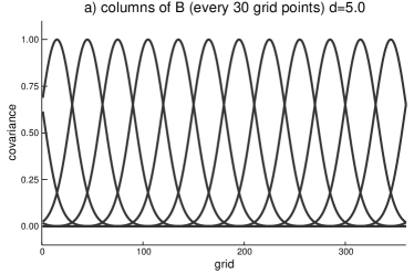
Figure 1: Structure of the true background error covariance matrix $\mathbf{B}$ for parameters (a) $d=5$ and (b) $d=20$. Each curve represents the column of $\mathbf{B}$ starting from the 15th column with a stride of 30. Larger values of $d$ correspond to narrower peaks.

As the background error covariance model, we follow the sinusoidal basis model given in the Appendix A.1 of Bishop and Hodyss (2009a). In this model, the covariance matrix is diagonalized in the space spanned by the sinusoids (sine and cosine curves) with wavenumbers at most $N_{\mathrm{grid}}/2$, and the eigenvalues are chosen such that each column (or raw) of the covariance matrix takes an identical Gaussian shape whose length scale is controlled by a parameter $d$. The variances at each grid point (the diagonal entries of the covariance matrix) are all set to one. Visual depiction is perhaps more helpful than the precise definition given with equations; instances of this covariance model, with parameter $d=5$ and 20, are shown in Figure 1. All the experiments shown below are performed with $d=20$ unless otherwise stated, but we have also repeated all the experiments with different choices of $d$ and confirmed that the results are qualitatively similar.

We assume that the state is observed at every 3 grid points including the first grid point indexed with 1, resulting in $p=120$ observations which can be represented by a $p$-dimensional column vector $\mathbf{y}^{o}$. We assume that the observation errors are uncorrelated and each observation share the same error variance ${\sigma^{o}}^{2}$, so that $\mathbf{R}={\sigma^{o}}^{2}\mathrm{I}_{p}$.

With this set-up, we conducted ETKF or LETKF assimilation experiments to investigate their properties in light of DFS argument. As a reference, we also conducted canonical KF analysis using the true error covariances. For each of the ETKF experiments, we stochastically generate the observations, the background mean and the background perturbations, respectively, by:

$$\mathbf{y}^{o} =\mathbf{H}\mathbf{x}^{\mathrm{true}}+\mathbf{R}^{1/2}\bm{\varepsilon}^{o}$$ (24)

$$\mathbf{x}^{b} =\mathbf{x}^{\mathrm{true}}+{\mathbf{B}^{\mathrm{true}}}^{1/2}\bm{\varepsilon}^{b}$$ (25)

$$\mathbf{X}^{b} ={\mathbf{B}^{\mathrm{true}}}^{1/2}\left[\bm{\varepsilon}_{1},\bm{\varepsilon}_{2},\cdots,\bm{\varepsilon}_{K}\right]$$ (26)

where $\mathbf{H}$ is the observation operator which picks up the values of the state vector $\mathbf{x}$ at every 3 grid points starting from the first (topmost) element of $\mathbf{x}$, $\mathbf{x}^{\mathrm{true}}$ is the hypothetical true state, ${\mathbf{B}^{\mathrm{true}}}^{1/2}$ is the symmetric square root of the true background error covariance matrix ${\mathbf{B}^{\mathrm{true}}}$ constructed as stated above, $K$ is the ensemble size, and the vectors $\bm{\varepsilon}^{o}\in\mathbb{R}^{p}$, $\bm{\varepsilon}^{b}\in\mathbb{R}^{N_{\mathrm{grid}}}$ and $\bm{\varepsilon}_{i}\in\mathbb{R}^{N_{\mathrm{grid}}}(i=1,\cdots,K)$ are random vectors, each entry of which is an independent draw from the standard normal distribution with mean zero and unit variance. The choice of the true state $\mathbf{x}^{\mathrm{true}}$ is irrelevant in this study, so we arbitrarily set it to a zero vector.

To highlight the relevance of DFS in terms of the ability of DA methods to extract observational information, we consider two different scenarios. In the first, “high DFS” scenario, we set $\sigma^{o}=1$. In this case, the observations are about as accurate as the background (recall that we chose $\mathbf{B}^{\mathrm{true}}$ so that each of its diagonal entries are one), meaning that observations should provide about the same amount of information as the background does. We have equally accurate sources of information from 360 background values and 120 observation, so that we can intuitively expect the optimal DFS to be close to $120/(120+360)$ times the number of observations (120), which is 30, and this is indeed not very different from the exact value of the optimal DFS which is 39.877. In the second, “low DFS” scenario, we set $\sigma^{o}=5$, so that observations are five times less accurate than the corresponding background. In this case, observations provide much less information compared to the background, so that the optimal DFS should be small. The exact value of the optimal DFS in this case is 4.386.

For each of the senario, we conduct ETKF experiments, with or without localization, using different ensemble sizes. In each experiment we conduct 1,000 trials changing the seed for the random number generator to ensure statistical robustness of the results.

In experiments that apply covariance localization, we use the 5th order piecewise rational function with finite support defined in Eq. (4.10) of Gaspari and Cohn (1999). This function becomes identically zero beyond a cut-off distance $d_{\mathrm{cut-off}}$, and hereafter we use this cut-off distance to specify the length scale of localization.

In the experiments discussed in section 4.3, we implemented B-localization as model-space B-localization through the ensemble modulation technique. We remark that, with our observation operator $\mathbf{H}$ that only picks up state variables at selected grid points, model-space and observation-space B-localization are equivalent.

4.2 Dependence on the ensemble size

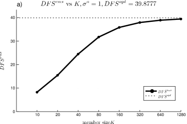
Figure 2: DFS attained by ETKF (or each local analysis of LETKF), $\mbox{DFS}^{\mathrm{ens}}$, plotted as a function of the ensemble size $K$, for (a) the “high DFS” and (b) “low DFS” scenarios. As a reference, the DFS that would be attained by an optimal canonical KF, $\mbox{DFS}^{\mathrm{opt}}$, is plotted in each panel as a horizontal dashed line.

We first examine cases without localization. The dependence of $\mbox{DFS}^{\mathrm{ens}}$ (averaged over 1,000 independent trials) on the ensemble size $K$ is depicted in Figure 2 together with $\mbox{DFS}^{\mathrm{opt}}$ that should be attained by the optimal canonical KF. In both “high DFS” (panel a) and “low DFS” (panel b) scenarios, $\mbox{DFS}^{\mathrm{ens}}$ monotonically increases as the ensemble size $K$ gets larger until it converges to $\mbox{DFS}^{\mathrm{opt}}$. In the “high DFS” scenario, approximately 200 members are required to achieve 90 % of $\mbox{DFS}^{\mathrm{opt}}$, whereas, in the “low DFS” scenario, the same level of saturation is achieved with only $\sim$50 members. This contrast is consistent with our expectation from the theory that a small ensemble size $K$ should be tolerated if $\mbox{DFS}^{\mathrm{opt}}$ is small (c.f., section 3.2).

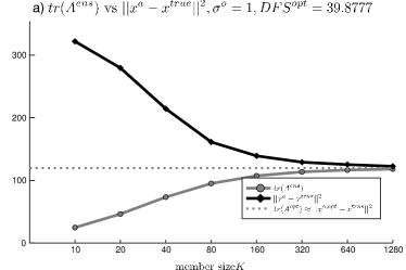
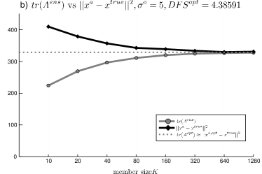
Figure 3: Trace of analysis error covariance $\mathrm{tr}\ \mathbf{A}^{\mathrm{ens}}$ (gray filled circle) and the analysis MSE (black filled square) for ETKF analysis (or each local analysis of LETKF) plotted as a function of the ensemble size $K$, for (a) the “high DFS” and (b) “low DFS” scenarios. As a reference, their counterpart obtained by an optimal canonical KF, is plotted in each panel as a horizontal dashed line.

The DFS diagnostics shown above is performed in the normalized observation space, but similar tendencies can also be observed in the model space. Figure 3 shows the trace of the analysis ensemble covariance, $\mathrm{tr}\ \mathbf{A}^{\mathrm{ens}}$, and the mean squared error (MSE) of the analysis mean, $\|\overline{\mathbf{x}}^{\mathrm{a,ens}}-\mathbf{x}^{\mathrm{true}}\|^{2}$, averaged over 1,000 trials, as a function of the ensemble size $K$. As a reference, their counterpart in an optimal canonical KF is also plotted with a dotted line. In both “high DFS” and “low DFS” scenarios, both $\mathrm{tr}\ \mathbf{A}^{\mathrm{ens}}$ and the analysis mean MSE converge to their optimal value as $K$ becomes large, but the former is consistently smaller than the latter. Recalling that $\mathrm{tr}\ \mathbf{A}^{\mathrm{ens}}$ is the estimate of the analysis mean MSE that is assumed by the assimilation algorithm, $\mathrm{tr}\ \mathbf{A}^{\mathrm{ens}}$ being smaller than the analysis MSE means that the analysis is overconfident. We can observe that, in both cases, the level of overconfidence diminishes as the ensemble size $K$ gets larger. Comparing the two scenarios, we can also observe that the overconfidence is much stronger in the “high DFS” scenario than in the “low DFS” scenario. These results corroborate our deduction from the theory that the ensemble size required to alleviate overconfidence in analysis should increase in proportion to $\mbox{DFS}^{\mathrm{opt}}$.

As discussed in section 3.2, underestimation of DFS is suggestive of underestimation of analysis increment. A plot (not shown) comparing the $l_{2}$-norm of analysis increment from ETKF, $\|\mathbf{K}^{\mathrm{ens}}\mathbf{d}\|$ as a function of the ensemble size $K$, with that of an optimal analysis, $\|\mathbf{K}^{\mathrm{opt}}\mathbf{d}\|$, exhibits a converging curve similar to the one shown in Figure 2, with the former consistently underestimating the latter, again corroborating the expectation from the theory.

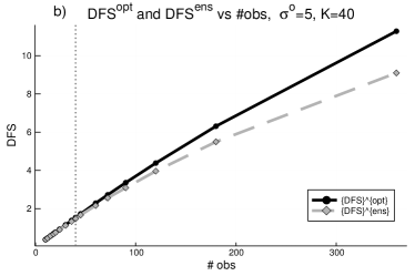
Figure 4: The DFS attained by ETKF with the ensemble size $K=40$ ($\mbox{DFS}^{\mathrm{ens}}$, gray dashed line) and the DFS attained by the optimal canonical KF ($\mbox{DFS}^{\mathrm{opt}}$, black solid line) plotted as a function of the number of observations, for (a) the “high DFS” and (b) “low DFS” scenarios. The vertical line in each panel shows the ensemble size $K=40$.

A plot similar to Figure 2 but with a fixed ensemble size ($K=40$) and varying the number of observations (Figure 4) is also illuminating. In the “high DFS” scenario, $\mbox{DFS}^{\mathrm{ens}}$ is close to $\mbox{DFS}^{\mathrm{opt}}$ when the number of observations $p$ is small, but as $p$ increase beyond the ensemble size $K=40$, the former begins to underestimate the latter. In contrast, in the “low DFS” scenario, $\mbox{DFS}^{\mathrm{ens}}$ stays close to $\mbox{DFS}^{\mathrm{opt}}$ even for very large values of $p$. This is because $\mbox{DFS}^{\mathrm{opt}}$ is well below the ensemble size ($K=40$) even for the fully observed case so that the $\mbox{DFS}^{\mathrm{ens}}$ being bounded by $K$ does not pose much limitation.

4.3 Role of localization

In section 3.3 we expounded on how the DFS underestimation that occurs if the ensemble size $K$ is much smaller than $\mbox{DFS}^{\mathrm{opt}}$ can be alleviated by localization. In this subsection we experimentally illustrate how the two localization methods differ in this respect.

4.3.1 B-localization

Recalling that DFS is the sum of all the eigenvalues $\lambda^{a}_{i}$ of the matrix $\mathbf{H^{\prime}AH^{\prime}}^{T}$, it is illuminating to examine how localization changes the eigenspectrum of this matrix.

The eigenvalues, sorted from the largest to the smallest, of the matrix $\mathbf{H^{\prime}A}^{\mathrm{opt}}\mathbf{H^{\prime}}^{T}$ computed using the true background covariance matrix with the canonical KF, are plotted in Figure 5 with the thick solid line. The true posterior eigenvalues smoothly decrease as the mode number gets higher and almost (but not exactly) vanishes at $\sim$ 100th and higher modes. Their ensemble equivalent, computed by raw ETKF without any localization using $\mathbf{B}^{\mathrm{ens}}$ constructed from 40 members (the thick dotted line), abruptly become zero at the 40th mode. This is an indication of DFS underestimation since the areas below these curves correspond to DFS.

Model space B-localization allows us to avoid this abrupt truncation of the eigenspectrum. The posterior eigenvalues, computed by ETKF using the modulated background ensemble (see section 3.3), are plotted with the thin solid line in Figure 5. Here, we manually tuned the localization scale to achieve minimal analysis mean MSE (giving $d_{\mathrm{cut-off}}=20\sqrt{10/3}\approx 36$), and the localization matrix $\bm{\rho}$ is approximated by retaining the leading $L=20$ eigen modes, which recovers 93.4% of the trace of the original matrix $\bm{\rho}$. We can observe that a well-tuned B-localization can almost perfectly recover the true posterior eigenspectrum, which means that DFS underestimation can be avoided.

The change in eigenspectrum caused by the use of B-localization can be better understood by noting the following (suggested by Dr. T. Tsuyuki; private communication): as we saw in section 3.3, the rank of $\mathbf{B}^{\mathrm{ens}}$, or eqivalently the number of non-zero eigenvalues $\lambda^{b}_{i}$ of $\mathbf{H}^{\prime}\mathbf{B}^{\mathrm{ens}}\mathbf{H}^{\prime T}$, increases from $K-1$ to $KL-1$ by applying B-localization. Now, recalling that model-space and observation-space B-localization are equivalent in this particular case where $\mathbf{H}$ only picks up state variables at selected grid points, the matrix $\mathbf{H}^{\prime}\left(\bm{\rho}\circ\mathbf{B}^{\mathrm{ens}}\right)\mathbf{H}^{\prime T}$ can be expressed as $\bm{\rho}_{\mathrm{obs}}\circ\left(\mathbf{H}^{\prime}\mathbf{B}^{\mathrm{ens}}\mathbf{H}^{\prime T}\right)$ by choosing an appropriate $p\times p$ correlation matrix $\bm{\rho}_{\mathrm{obs}}$. Since all the diagonal entries of $\bm{\rho}_{\mathrm{obs}}$ are one, it follows that $\sum_{i=1}^{K-1}\lambda^{b,\mathrm{raw}}_{i}=\mathrm{tr}\ \mathbf{H}^{\prime}\mathbf{B}^{\mathrm{ens}}\mathbf{H}^{\prime T}=\mathrm{tr}\ \bm{\rho}_{\mathbf{obs}}\circ\left(\mathbf{H}^{\prime}\mathbf{B}^{\mathrm{ens}}\mathbf{H}^{\prime T}\right)=\sum_{i=1}^{KL-1}\lambda^{b,\mathrm{loc}}_{i}$, where $\lambda^{b,\mathrm{raw}}_{i}$ and $\lambda^{b,\mathrm{loc}}_{i}$ denote, respectively, the eigenvalues of the prior error covariance matrix measured in the normalized observation space before and after application of B-localization. This means that the sum of all the eigenvalues of the prior error covariance is invariant under application of B-localization, while the number of its non-zero elements increases $L$-fold, which implies that B-localization reduces the larger eigenvalues while increasing the smaller eigenvalues including those that are null, leading to flattening of the prior eigenspectrum. Consequently, the posterior eigenspectrum is also flattened by B-localization since the posterior eigenvalue $\lambda^{a}_{i}$ as a function of the prior eigenvalue $\lambda^{b}_{i}$ is monotonically increasing (see Equation 12), which explains how the posterior eigenspectrum is deformed by B-localization from the gray thick dotted line to the thin black solid line shown in Figure 5.

4.3.2 R-localization

R-localization circumvents this DFS underestimation issue in a different manner. As we saw in section 3.3, with R-localization, $\mbox{DFS}^{\mathrm{ens}}$ is inevitably smaller than the ensemble size so DFS underestimation is unavoidable as long as $\mbox{DFS}^{\mathrm{opt}}$ is greater than the ensemble size. Instead of solving the full data assimilation problem using the full $\mathbf{B}$ matrix, localized EnKF algorithms like LETKF divide the domain into smaller pieces exploiting the localized structure of the background error covariance (i.e., the block diagonality of the $\mathbf{B}$ matrix) and solves smaller data assimilation problems using the diagonal submatrices of $\mathbf{B}$ (Evensen, 2004; Ott and Coauthors, 2004). The resultant smaller data assimilation problems are solved independently for each local domain. In our simple covariance model with the parameter $d=20$ (Figure 1b) , for example, the $\mathbf{B}$ matrix assumes localized structure with almost zero correlations beyond $\sim 15$ grid points apart, so that, when performing analysis for a particular grid point, limiting the domain to the neighboring grid points within some radius (called cut-off distance hereafter) greater than $\sim 15$ and then performing data assimilation, neglecting all background field and observations outside this local domain, should yield analysis close to what would be obtained with global analysis using full background field and observations. This is exactly how data assimilation is performed with LETKF. This way the number of locally assimilated observations can be reduced (Hunt et al., 2007), resulting in $\mbox{DFS}^{\mathrm{opt}}$ for the localized problem being smaller than the ensemble size if the cut-off distance is chosen small enough, thus allowing us to circumvent the DFS underestimation issue.

In the case we are considering (with parameter $d=20$ and the ensemble size $K=40$), the optimally-tuned cut-off distance for R-localization was $d_{\mathrm{cut-off}}=14\sqrt{10/3}\approx 26$, in which case the number of the locally assimilated observations is restricted to only $17(\approx(2\times 26+1)/3)$. The gray thick solid line plotted in Figure 6 shows the eigenvalues of the posterior error covariance matrix projected onto the normalized observation space $\mathbf{H^{\prime}}_{\mathrm{loc}}\mathbf{A}_{\mathrm{loc}}^{\mathrm{opt}}\mathbf{H^{\prime}}_{\mathrm{loc}}^{T}$ computed by the optimal canonical KF restricted to this localized domain (here the matrix $\mathbf{H^{\prime}}_{\mathrm{loc}}$ denotes a normalized observation operator similar to $\mathbf{H^{\prime}}$ but which selects only the observations whose distances from the analyzed grid point are below the cut-off distance). Here we arbitrarily show the result for the localized problem centered around the first grid point but the results are insensitive to the choice of the analyzed grid point because of the translational symmetry of our covariance model. Note that the eigenvalues are zero beyond the 18th mode since the rank of the matrix $\mathbf{H^{\prime}}_{\mathrm{loc}}\mathbf{A}_{\mathrm{loc}}^{\mathrm{opt}}\mathbf{H^{\prime}}_{\mathrm{loc}}^{T}$ is only 17 (the number of locally assimilated observations). Their ensemble equivalent computed with raw ensemble covariance but with the domain localization (gray thick dotted line) is close to the optimal one unlike in the case of full domain (compare with Figure 5). When R-localization is applied, the posterior eigenvalues become smaller than when only domain localization is applied (black thin dotted line), meaning that R-localization actually leads to smaller DFS than without. This is consistent with the finding of Huang et al. (2019) who also provided a mathematical explanation.

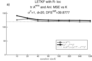
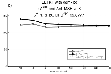
Figure 8: As in Figure 3a, but for LETKF with (a) R-localization together with domain localization, and (b) domain localization only. For each ensemble size $K$, the localization parameter $d_{\mathrm{cut-off}}$ is manually tuned to yield the smallest analysis MSE with respect to the truth.

By working with the localized domain, the DFS underestimation is mostly mitigated, and so is the overconfidence in the analysis spread. The panels (a) and (b) in Figure 8 show, respectively, a plot similar to Figure 3a but for optimally-tuned LETKF with R-localization (together with its inherent domain localization), and the same plot but with domain localization only. Comparing these with Figure 3a, it is evident that LETKF analyses suffer much less from overconfidence issue than the raw ETKF without any localization (Figure 3a), and that the analysis MSE close to that of the optimal KF is achieved with much smaller ensemble sizes, proving the effectiveness of domain localization. Interestingly, for this particular simple problem, the benefit of R-localization appears to be mostly attributable to the use of domain localization, as we can infer by comparing Figures 8a and 8b which show very similar performances. Note that we should not discredit the advantage of R-localization over domain localization simply based on these results. R-localization is known to have the advantage of ensuring spatially smoother (and thus better balanced) analysis than simple domain localization does. This advantage is particularly important in a cycled context (Greybush et al., 2011), but is totally dismissed in our problem setup.

In LETKF with R-localization or domain localization, the Kalman gain for the global analysis in full domain (denoted $\mathbf{K}^{\mathrm{LEKTF}}$ hereafter), or the analysis error covariance implied by $\mathbf{K}^{\mathrm{LEKTF}}$, are not explicitly available in algebraic matrix form, but it is possible to numerically compute them row-wise if we note that each row (say the $i$-th row) of the global Kalman gain $\mathbf{K}^{\mathrm{LEKTF}}$ is computed in the local analysis centered around the $i$-th grid point as the row of local Kalman gain that corresponds to the center of this local analysis. The row from the local Kalman gain is shorter than the corresponding row of the global Kalman gain, so the components of the latter that corresponds to the observations that are outside the truncated local domain have to be padded with zero. Once $\mathbf{K}^{\mathrm{LEKTF}}$ is thus computed, a counterpart of Figure 5 can be produced, albeit with several caveats to be kept in mind.

In the global analysis of LETKF, the optimality of the Kalman gain (in the sense of Equation 6 being strict), while being valid for each local domain, does not globally hold exactly, which means that Equation 4 and thus Equation 5 are not valid. Accordingly the equivalence of $\mathbf{H^{\prime}AH^{\prime}}^{T}$ and $\mathbf{R}^{-1/2}\mathbf{HK}\mathbf{R}^{1/2}$ does not hold for the global analysis, making it difficult to interpret the DFS (defined as the trace of $\mathbf{HK}$) as the posterior error variance represented by the assimilation scheme. Another difficulty that follows from Equation 6 being not exact is that $\mathbf{R}^{-1/2}\mathbf{HK}^{\mathrm{LETKF}}\mathbf{R}^{1/2}$ is not assured to be symmetric, resulting in their eigenvalues not necessarily real values. An easy remedy to this is to focus on its symmetric component

$$\mathbf{H^{\prime}K^{\prime}}^{\mathrm{LETKF},S}:=\frac{1}{2}\left\{\left(\mathbf{R}^{-1/2}\mathbf{HK}^{\mathrm{LETKF}}\mathbf{R}^{1/2}\right)+\left(\mathbf{R}^{-1/2}\mathbf{HK}^{\mathrm{LETKF}}\mathbf{R}^{1/2}\right)^{T}\right\}$$ (27)

and investigate its eigenspectrum (suggested by Dr. T. Tsuyuki; private communication). This remedy may seem ad hoc but is justified by the following two properties: Firstly, it conserves the trace and thus respects the identity

$$\mathrm{tr}\ \mathbf{H^{\prime}K^{\prime}}^{\mathrm{LETKF},S}=\mathrm{tr}\ \mathbf{R}^{-1/2}\mathbf{HK}^{\mathrm{LETKF}}\mathbf{R}^{1/2}=\mathrm{tr}\ \mathbf{HK}^{\mathrm{LETKF}}=\mbox{DFS}^{\mathrm{ens}}.$$ (28)

Secondly, by focusing on the symmetric component, the requirement that eigenvalues $\lambda^{a}_{i}$ of $\mathbf{H^{\prime}K^{\prime}}^{\mathrm{LETKF},S}$ should lie between 0 and 1 can be interpreted intuitively as requiring that the analysis should be an interpolation between the first guess and the observation. To see why the second point holds, recall that the observation-space inner product (scaled by $\mathbf{R}^{-1}$) between the innovation vector and the analysis increment can be expressed as

$$\left(\mathbf{y}^{o}-\mathbf{y}^{b}\right)^{T}\mathbf{R}^{-1}\left(\mathbf{y}^{a}-\mathbf{y}^{b}\right)=\mathbf{d}^{T}\mathbf{R}^{-1}\left(\mathbf{y}^{a}-\mathbf{y}^{b}\right)=\mathbf{d}^{T}\mathbf{R}^{-1}\mathbf{HK}^{\mathrm{LETKF}}\mathbf{d}=\mathbf{d^{\prime}}^{T}\mathbf{R}^{-1/2}\mathbf{HK}^{\mathrm{LETKF}}\mathbf{R}^{1/2}\mathbf{d^{\prime}}$$

$$=\frac{1}{2}\left\{\left(\mathbf{d^{\prime}}^{T}\mathbf{R}^{-1/2}\mathbf{HK}^{\mathrm{LETKF}}\mathbf{R}^{1/2}\mathbf{d^{\prime}}\right)+\left(\mathbf{d^{\prime}}^{T}\mathbf{R}^{-1/2}\mathbf{HK}^{\mathrm{LETKF}}\mathbf{R}^{1/2}\mathbf{d^{\prime}}\right)^{T}\right\}=\mathbf{d^{\prime}}^{T}\mathbf{H^{\prime}K^{\prime}}^{\mathrm{LETKF},S}\mathbf{d^{\prime}}$$ (29)

where $\mathbf{y}^{b}:=\mathbf{Hx}^{b}$ is the first guess in the observation space and $\mathbf{d^{\prime}}:=\mathbf{R}^{-1/2}\mathbf{d}$ is the normalized innovation vector. Since the eigenvalues $\lambda^{a}_{i}$ are the factors by which the vector $\mathbf{d^{\prime}}$ magnifies or shrinks in the corresponding eigen-directions when multiplied from left by $\mathbf{H^{\prime}K^{\prime}}^{\mathrm{LETKF},S}$, if $0<\lambda^{a}_{i}<1$ holds for all $i$, that implies that, taking $\mathbf{y}^{b}$ as the origin in the normalized observation space, in any direction, $\mathbf{y}^{a}$ never goes beyond $\mathbf{y}^{o}$ nor does it lie in the opposite side of $\mathbf{y}^{o}$ with respect to the origin $\mathbf{y}^{b}$, or stated differently, $\mathbf{y}^{a}$ is an interpolation between $\mathbf{y}^{b}$ and $\mathbf{y}^{o}$.

The eigenspectrum of $\mathbf{H^{\prime}K^{\prime}}^{\mathrm{LETKF},S}$, computed with the optimally-tuned R-localization or with the domain localization only, are plotted in Figure 7. Similarly to B-localization (see Figure 5), R-localization and domain localization successfully restore the true eigenspectrum (gray thick solid line), attesting the effectiveness of R-localization or domain localization in the context of global analysis. Interestingly again, the two curves (for R-localization and domain localization) exhibit very similar pattern, suggesting that much of the benefit of R-localization can be achieved by domain localization alone. Since the underestimation of $\mathrm{tr}\ \mathbf{HK}$ (the area below the curves) is alleviated, we can expect that R-localization or domain localization should alleviate the underestimation of the analysis increment ($\mathbf{HKd}$ or $\mathbf{Kd}$). We confirmed that this is indeed the case in our experiment: the ratio of the $l_{2}$-norm of analysis increment computed by ETKF (averaged over 1,000 trials) divided by the same quantity computed by the optimal canonocal KF increased from 0.7 to 0.9. We remark that, since the identity between $\mathbf{H^{\prime}K^{\prime}}^{\mathrm{LETKF},S}$ and $\mathbf{H^{\prime}AH^{\prime}}^{T}$ does not necessarily hold for global analysis of LETKF, the mitigation of DFS (the sum of all $\lambda^{a}_{i}$) cannot be immediately interpreted as mitigation of posterior underdispersion (although from Figure 8 it does seem quite likely to be mitigated).

5 Discussions: interpretation of results from the literature in light of DFS

In the literature of atmospheric data assimilation studies, especially those on operational implementation of LETKF, several interesting findings have been reported and some of them appear to be counter-intuitive. This section is devoted to discussing how DFS-based arguments developed in the preceding sections could help interpret such seemingly puzzling findings. The discussions given here are admittedly highly speculative, but the authors wish nonetheless to present them in hopes of stimulating further discussions by the community.

5.1 Using less is better

Among the many findings (or caveats) on operational or real-world implementations of LETKF, perhaps the most intriguing is the fact that assimilating less observations can lead to more accurate analysis or forecast. For example, Hamrud et al. (2015) developed quasi-operational implementation of both LETKF and serial ensemble square-root filter (EnSRF Whitaker and Hamill, 2002) coupled with the European Centre for Medium-range Weather Forecasts (ECMWF)’s operational forecast model (Integrated Forecast System; IFS) and found that, for LETKF, a very large forecast improvement is achieved by severely limiting the number of assimilated observations in the local analysis step for each analyzed grid point. They reported that, reducing the average number of locally assimilated observations $\sim 30$-fold from the original $\sim 40,000$ to only $\sim 1,200$ yields the best results and that the forecast performance is not very sensitive to the exact choice of the strength of number reduction. Curiously, they found this method (which they call “implicit covariance localization”) to be useful only for LETKF (with R-localization) and not for serial EnSRF (with observation-space B-localization).

The LETKF implementation for convective-scale data assimilation developed by Schraff and Coauthors (2016) takes a similar approach where, for each local analysis, the horizontal localization length-scale is adjusted so that the number of locally assimilated observations become constant (roughly double the ensemble size) at every analyzed grid point. Guo-Yuan Lien et al. (2017; private communication) applied a similar method to assimilation of phased array weather radar (PAWR) data by their LETKF (Lien et al., 2017) and confirmed that limiting the number of locally assimilated observations to a few times the ensemble size leads to significantly better forecast than assimilating all data or applying a traditional thinning method before assimilating them.

The fact that using less observations (i.e., discarding many of the available observations) leads to better forecast performance is, naively, not easily justifiable, but the theory of DFS applied to EnKF (see section 3) allows us a clear interpretation: $\mbox{DFS}^{\mathrm{ens}}$ is locally at most $K\textendash 1$ (where $K$ is the ensemble size), so that locally assimilating much more than $K$ observations results in overconfident analysis spread (requiring unreasonably large inflation) and smaller-than-optimal analysis increment. The above interpretation is not necessarily new, and we note that Schraff and Coauthors (2016) presents a similar heuristic argument as a rationale for their approach.

One may argue that the benefit of assimilating less observations should be attributable to the observations being sparser and thus less affected by the error correlation between different observations. However, such an interpretation seems not to apply here, because, in all of the three studies mentioned above, the observations that are spatially closest to the analyzed grid point are selected, so that the issue of correlated observation errors, if any, was not addressed by limiting the number of locally assimilated observations.

5.2 Relationship between the optimal localization scale and the ensemble size

The argument above suggests a convenient guidance on how to tune the localization scale in the context of LETKF with R-localization:
the localization scale should be as large as possible to keep the localized problem close to the original global problem, but subject to the condition that it is small enough so that the number of locally assimilated observations does not exceed several times the ensemble size (to ensure that locally $\mbox{DFS}^{\mathrm{opt}}<K$ holds).

This rule of thumb is again not new, and the insightful review paper by Tsyrulnikov (2010) developed a similar heuristic argument based in part on Lorenc (2003) to reach at a similar conclusion. Quoting from section 4.3 of Tsyrulnikov (2010), he reasoned that the optimal localization scale occurs when local analysis domain is small enough so that “ensemble size (is) commensurable with the number of observed degrees of freedom within an effective box.” In his discussion, the “observed degrees of freedom” has not been given a precise definition; we assert that DFS gives it a more precise definition. Tsyrulnikov (2010) further conducted meta-analysis of the published literature and found that the optimal localization scales that were experimentally determined in earlier studies do match this rule of thumb.

Covariance localization has traditionally been regarded as a means to alleviate the rank deficiency issue of the ensemble background error covariance matrix $\mathbf{B}^{\mathrm{ens}}$ (e.g., Houtekamer and Zhang, 2016) or a means to damp the sampling noises of $\mathbf{B}^{\mathrm{ens}}$(e.g., Ménétrier et al., 2015). From this perspective, it appears that determination of the optimal localization length scale is a problem intrinsic to the ensemble size $K$ and the structure of the true $\mathbf{B}$, independent of $\mathbf{H}$ or $\mathbf{R}$ (i.e., how the observations are distributed or how they are accurate). Interestingly, however, contrary to this traditional view, there have been ample evidence from the literature that suggests that the distribution and/or accuracy of observations are the key in determining the optimal localization scales in the context of LETKF with R-localization and domain localization. The theory based on DFS presented in this paper may help to reconcile this apparent contradiction.

5.3 Covariance inflation

Along with localization, covariance inflation is an indispensable component of practical EnKF implementation that is often performed in an ad hoc manner despite its importance. The concept of DFS is useful in explaining/justifying some of the inflation methods that were found effective in previous literature.

Wang et al. (2007) experimentally observed that the regular ETKF (as formulated in Bishop et al., 2001; Wang et al., 2004) systematically underestimates the posterior error variance if $K\ll r$ where $K$ is the ensemble size and $r$ is the rank of the true background error covariance $\mathbf{H^{\prime}}\mathbf{B}^{\mathrm{true}}\mathbf{H^{\prime}}^{T}$ projected onto the normalized observation space. Motivated by this observation, and guided by a series of insightful educated guesses (see their Appendix A), Wang et al. (2007) introduced an “improved ETKF” formulation which inflates the eigenvalues $\lambda^{b}_{i}$ of the sample prior error covariance projected onto the normalized observation space before computing the ensemble transform matrix. The inflation factor they derived has a rather complex expression but its key property is that it approaches $r/K$ (the rank of $\mathbf{H^{\prime}}\mathbf{B}^{\mathrm{true}}\mathbf{H^{\prime}}^{T}$ divided by the ensemble size) under some assumptions. The chain of logic behind their derivation is somewhat complicated, but the DFS argument given in section 3.2 of this manuscript allows us an intuitive (albeit heuristic) interpretation: when $K\ll r$, DFS (and thus the posterior error variance measured in the normalized observation space) should be underestimated ($\mbox{DFS}^{\mathrm{ens}}\ll\mbox{DFS}^{\mathrm{opt}}$) since $\mbox{DFS}^{\mathrm{ens}}<K-1\ll r$ and $r/\mbox{DFS}^{\mathrm{opt}}\sim O(1)$ if observations are accurate enough. We can recover the correct posterior variance by inflating $\mbox{DFS}^{\mathrm{ens}}$ by a factor $\mbox{DFS}^{\mathrm{opt}}/\mbox{DFS}^{\mathrm{ens}}$, and a simple way to do this is to inflate all the prior eigenvalues $\lambda^{b}_{i}$ by the same factor $\mbox{DFS}^{\mathrm{opt}}/\mbox{DFS}^{\mathrm{ens}}$. This factor is difficult to estimate since $\mbox{DFS}^{\mathrm{opt}}$ is usually unknown (in fact Wang et al. (2007) derived quite an elaborate expression to estimate this factor), but provided that $K\ll r$, it should be reasonable to assume that it is roughly proportional to $r/K$.

As we mentioned in section 3.3, Bishop et al. (2017) proposed the Gain-form ETKF (GETKF) that enables model-space B-localization in the ETKF framework. They observed that GETKF tend (though not always) to underestimate the posterior error variance in comparison to METKF (the ETKF that updates all the modulated ensemble members) and proposed to apply the “inherent GETKF inflation” which inflates each of the GETKF’s posterior perturbations by a constant factor $a$ that restores the model-space posterior variance of METKF. With experiments using a one-dimesional toy system repeated with various localization length scales, they found that:

• (a) the inherent inflation factor $a$ increases monotonically with the localization scale, and

• (b) interestingly, analysis becomes most accurate when the localization length scale is such that it neutralizes the inherent inflation factor (i.e., $a\approx 1$ holds).

The point (a) above is easier to understand if we note, from the DFS theory, that the larger the localization scale is, the more observations are assimilated, leading to severer DFS (and thus posterior variance) underestimation, requiring stronger covariance inflation. Bishop et al. (2017) acknowledges the potential significance of point (b) suggesting that it could be exploited to adaptively optimize localization scale if it is a generally applicable property. Bishop et al. (2017) were deliberate in stating that the validity of this hypothesis is left to future assessment, but the implication discussed in section 3.2 together with the similar evidence from literature summarized in Tsyrulnikov (2010), make it all the more likely.

Finally, among the many inflation methods, a family of “relaxation to prior” approaches have been found to be particularly effective. This family of inflation methods modify (inflate) the posterior ensemble after the analysis update has been made by relaxing the posterior perturbations themselves to the prior perturbations (Relaxation to Prior Perturbations; RTPP Zhang et al., 2004) or by relaxing the posterior spread to the prior spread (Whitaker and Hamill, 2012, Relaxation to Prior Spread; RTPS). While there can be many reasons why these relaxation approaches are effective, one important characteristic of them appears to be their ability to apply stronger inflation when and where the assimilated observations are distributed more densely, as pointed out by Whitaker and Hamill (2012). The DFS underestimation (or analysis overconfidence) that occurs when assimilating much more observations than the ensemble size, lends itself to justify the success of the relaxation approaches.

6 Summary and concluding remarks

Aiming at understanding how EnKF effectively extracts information from observations, in this paper we adapted the theory of DFS to EnKF algorithms with particular focus on the ETKF framework. Simple mathematical arguments based on elementary linear algebra revealed that, with EnKF algorithms, DFS is bounded from above by the ensemble size, which means that DFS is always underestimated when assimilating much more observations than the available ensemble size. This problem has long been recognized by the community and is referred to as the “rank deficiency issue” but it appears to have been rather vaguely defined. DFS argument allows us to describe this issue in a more quantitative manner.

The fact that DFS is underestimated when assimilating much more observations than the ensemble size has several important implications on the effectiveness of practical EnKF implementations, notably:

• Strong covariance inflation is necessary when assimilating much more observations than the ensemble size, which follows from the fact that DFS coincides with the analysis (posterior) variance measured in the normalized observation space, so that, if DFS is underestimated, the analysis spread becomes underdispersive (or equivalently, analysis becomes overconfident).

• DFS underestimation (or analysis overconfidence) can be avoided by imposing stronger localization when/where observations are denser. This comes at the expense of discarding some of the information from observations, but the merit of alleviating the overconfidence in analysis can outweigh such disadvantage.

These findings are not new, and similar arguments have been repeatedly made in the literature (e.g., Lorenc, 2003; Tsyrulnikov, 2010; Furrer and Bengtsson, 2007), but the authors believe that the DFS-based argument presented here helps us to understand the issue more clearly and more quantitatively.

The concept of DFS also allows us to understand how different localization schemes help to circumvent the DFS underestimation or analysis overconfidence. The implications from the DFS theory in this context have been explored and showcased using idealized experiments with a one-dimensional toy problem.

The examination on the role of localization based on the DFS concept highlights the advantage of B-localization over R-localization (i.e., being less susceptible to the problem of DFS underestimation or analysis overconfidence). In the previous studies, the benefit of using model-space B-localization, through the modulated ensemble approach in particular, have been emphasized in connection to its ability to correctly account for non-local observations like satellite radiances for which the position of the observation is ill-defined and thus R-localization cannot be clearly formulated (Bishop et al., 2017; Lei et al., 2018). The discussion given in this paper suggests the merit of B-localization beyond its intended advantage of correctly accounting for non-locality of observations.

Finally, several speculative arguments have been presented based on DFS theory about how some of the interesting results on (L)ETKF reported in the previous literature can be explained or justified in light of DFS concept. Intriguing questions such as why using less observations can be better, which localization length scales tend to be optimal, and why covariance inflation schemes based on “relaxation to prior” approaches are successful, all become easier to interpret by noting when DFS underestimation issue occurs. We remark that the theoretical argument and the discussions on the results from the idealized experiments presented in this paper only bring out the issues that (L)ETKF algorithms are subject to even when strong simplifying assumptions are satisfied, such as: the model and observation operator are both linear, the background and observation errors obey Gaussian distributions, the observation errors are uncorrelated, and $\mathbf{B}$ and $\mathbf{R}$ are perfectly known. Practical applications like real-world NWP bear many other complicating factors, so we need to be careful not to extrapolate too much from the simple theoretical arguments presented in this paper. The authors believe nevertheless that the findings shown here provide some useful insights.

Most DA methodologies studied in the atmospheric science or geophysics literature have assumed, implicitly or explicitly, that the system dimension is by far greater than the number of observations or the ensemble size (#ens $\sim$ #obs $\ll$ #grid) often emphasizing the underdetermined nature of DA problems. With the advent of meteorological Big Data, however, this assumption will no longer be justifiable. The situation that we should consider now is cases where there are about as many observations as the system dimension which by far exceed the affordable member size (i.e., #ens $\ll$ #obs $\sim$ #grid). The authors hope that the DFS concept will prove useful in developing DA methods suitable for this new emerging (or incoming) situation.

CONFLICT OF INTEREST

Authors declare no conflict of interest.

Appendix: DFS diagnostics applied to a quasi-operational global LETKF

Introduction

The Degrees of Freedom for Signal (DFS), or analysis sensitivity to observations, first introduced to NWP by Cardinali (2004) and Fisher (2003), is a convenient measure of how much of information content a particular data assimilation (DA) system can extract from different types of observations. Diagnostics of this quantity is useful in identifying issues or limitations of a data assimilation system, observation error specification, or of observations themselves. In this Appendix, we briefly show the results from DFS diagnostics applied to a quasi-operational version of global LETKF system developed at Japan Meteorological Agency (JMA).

DFS calculation

Following Liu et al. (2009), DFS is calculated from the analysis perturbations mapped onto the observation space, $\mathbf{Y}^{a}=\mathbf{HX}^{a}$, using

$$\mbox{DFS}^{\mathrm{ens}}=\mathrm{tr}\ \mathbf{HK}=\mathrm{tr}\ \mathbf{H}\mathbf{A}^{\mathrm{ens}}\mathbf{H}^{T}\mathbf{R}^{-1}=\left(\mathbf{R}^{-1/2}\mathbf{Y}^{a}\right)^{T}\left(\mathbf{R}^{-1/2}\mathbf{Y}^{a}\right)/(K-1).$$ (A1)

In our system, the prescribed observation error covariance matrix $\mathrm{R}$ is chosen to be diagonal, so the DFS as calculated above can be divided into contributions from each observation (which are just the sample analysis variance corresponding to each observation normalized by the corresponding observation error variance). Then, for each subset of observations grouped by each instrument or each observed type, we can define “DFS per observation” (which is also referred to as “self sensitivity”; see Cardinali (2004) for detail). Monitoring of the per-obs DFS thus defined for different observation types is a very useful diagnostics.

Experimental setup

The DA system analyzed here is a pre-operational version of JMA’s global LETKF that is operated to produce the initial perturbations used in the global ensemble prediction system (Yamaguchi et al., 2018). It is a 50-member LETKF system, each member of which is a lower-resolution run (TL319 in horizontal, $\sim 60$ km grid spacing, and 100 vertical levels reaching from the surface up to 0.01 hPa) of JMA’s Global Spectral Model (GSM). At the end of each analysis update, the analysis mean is recentered to the deterministic higher-resolution analysis produced by 4DVar. A detailed description of this LETKF system is given in section 3.3.3.1 of JMA (2019).

In this experiment, all the types of observations that are used operationally by 4DVar are assimilated by the LETKF. The assimilated observations are grouped into the following categories: SYNOP (surface pressure measurements from ground-based stations), SHIP (surface pressure measurements over the seas reported from vessels or moored buoys), BUOY (as in SHIP but from drifting buoys), RADIOSONDE (upper-level sounding observations of pressure, temperature, winds and humidity reported from radiosondes), PILOT (upper-level wind observations from rawin or pilot balloons), AIRCRAFT (aircraft observations reported via AIREP or AMDAR programme), TYBOGUS (typhoon bogus data), PROFILER (wind profiles measured from ground-based radars), GNSS-DELAY (zenith total delay observations from ground-based GNSS receivers), GNSS-RO (GNSS radio occultation observed by low earth orbit satellites), AMVGEO (upper-level winds inferred as atmospheric motion vectors from geostationary satellite imagery), AMVLEO (as in AMVGEO but from lower earth orbit satellites), AMSU-A (microwave radiance soundings from AMSU-A sensors), AIRS (hyper-spectral infrared sounding from AIRS sensor), MHS (microwave humidity sounding from MHS sensors), IASI (hyper-spectral infrared sounding from IASI sensor), SCATWIND (ocean surface wind vectors inferred from ASCAT scatterometers), TMI (microwave imagery from TMI sensor onboard TRMM satellite), AMSR2 (microwave imagery from AMSR2 sensor onboard GCOM-W satellite), SSMIS (microwave imagery from SSMIS sensors) and CSR (clear sky radiance imagery from water-vapor-sensitive channels of geostationary satellites). The details on these observations are documented in Section 2.2 of JMA (2013) or JMA (2019).

The results shown here are based on the statistics taken from the 5-day period from 06 UTC, 10 July 2013 to 00 UTC, 15 July 2013. Just five days may not be long enough for a reliable statistics, but we have confirmed that the DFS statistics are not too different for different periods from different seasons; to make the appendix concise, we only focus on this particular 5-day period.

Overview of the results

To gain insight as to which observation types are most informative in terms of information content, we first examine the relative (fractional) contributions from each observation type to the total DFS, defined as the sum of DFS for each observation within each group divided by the total DFS (the sum of DFS for all observations), which are plotted in Figure A1. The DFS is most contributed by AMSU-A and GNSS-RO observations which together account for more than half of the total DFS, followed by CSR, RADIOSONDE and AIRCRAFT. We highlight here that contributions from hyper-spectral soudings (AIRS and IASI) are relatively small despite that they dominate in terms of the data volume (the number of observations); this is in stark contrast to recent DFS results from variational analysis at ECMWF (Cardinali, 2013) and Météo France , for instance, where a large contribution from hyper-spectral sounders (notably IASI) is reported.

The mean per-obs DFS, defined as $\mathrm{tr}\ \mathbf{HK}/p$ where $p$ is the number of all the assimilated observations, is a measure of how much of information the analysis extracts from observations on average. In some literature (e.g. Cardinali, 2004; Lupu et al., 2011) this is called Observation Influence (OI). The mean per-obs DFS for our LETKF system was only 0.0157 (1.57%), meaning, to the authors’ surprise, that the LETKF analysis relies about 98% on the information from the background. This is very small compared to results from variational systems. For example, in a recent study from ECMWF’s 4DVar, the mean per-obs DFS was $\sim$ 11% (Cardinali, 2013); similarly, Lupu et al. (2011) reported that the mean per-obs DFS at Canadian operational 4DVar was about 10%. In an idealized Observing System Simulation Experiment (OSSE) using an intermediate global atmospheric model where rather sparse in-situ observations are assimilated by LETKF (Liu et al., 2009), the mean per-obs DFS was about 15%. As we show in the next paragraph, the smallness of the mean per-obs DFS can be attributed to the small per-obs DFS for hyper-spectral sounders (AIRS and IASI) that constitute more than 70% of the total observation count.

Figure A2 plots the per-obs DFS (or self sensitivity) calculated for different types of observations, using samples taken from (a) entire globe, (b) Tropics, (c) Northern Hemisphere extratropics (NH), and (d) Southern Hemisphere extratropics (SH). In any of the regions, conventional (non-radiance) observations tend to have higher per-obs DFS than satellite radiance observations (except for CSR which are assigned relatively small error variance and are relatively sparse compared to other radiance data due to the cloud-freeness constraint and the strong horizontal thinning that picks only one observation in a 200 km $\times$ 200 km box). Notably, isolated observations like BUOY and SHIP exhibit large per-obs DFS. It can be also observed that per-obs DFS for conventional observations (like SYNOP, SHIP, BUOY and RADIOSONDE) are larger in SH and Tropics than in NH. These features are consistent with Cardinali (2004) who showed that isolated observations tend to show larger DFS.

What is striking in Figure A2, in comparison to similar diagnostics from variational DA systems (e.g., Cardinali (2013) and the real-time monitoring at Météo France) is that per-obs DFS for hyper-spectral sounders (AIRS and IASI) are very small. We discuss this point in the next subsection.

Discussion

The formula for computing DFS applicable to any EnKF algorithm has been devised in Liu et al. (2009) but appears not to have been applied to an operational EnKF implementation. Here a DFS diagnostics is applied perhaps for the first time to a quasi-operational global LETKF implementation that assimilates all types of observations that are operationally assimilated by 4DVar.

The striking feature of the DFS diagnosed for LETKF, in comparison to those reported for variational DA systems in the literature, is that the mean per-obs DFS is very small. This feature is largely attributable to the smallness of per-obs DFS for AIRS and IASI that constitute more than 70% of the total data count. The important question then is to understand why DFS is so small for these types of observations.

From the classical theory of DFS (Cardinali, 2004; Fisher, 2003) (which assumes that the Kalman gain $\mathbf{K}$ is accurately computed from $\mathbf{B}$ and $\mathbf{R}$), in order for DFS to be small, the observation error variance has to be large in comparison to its counterpart from the background. In our LETKF, the observation error covariance $\mathbf{R}$ is identical to what is used in the operational 4DVar, while the background error variance (as inferred from the background ensemble spread) tends to be smaller than its counterpart prescribed in 4DVar by a factor of $\sim 2^{2}$ or $3^{2}$. This discrepancy in the magnitude of $\mathbf{B}$ is perhaps a factor contributing to the discrepancies in DFS between LETKF and 4DVar in general, but it alone cannot explain why per-obs DFS in LETKF are reasonably large for sparse observations like BUOY and SHIP but are disproportionately small for AIRS and IASI. It appears then that, to understand and explain the discrepancy in DFS for AIRS and IASI between LETKF and 4DVar, we need to examine how the Kalman gain $\mathbf{K}$ is computed in these two algorithms. This question motivated the study presented in the main part of this manuscript.

Figures

Figure 5: Eigenvalues of the matrix $\mathbf{H^{\prime}A}^{\mathrm{opt}}\mathbf{H^{\prime}}^{T}$ (gray thick solid line), $\mathbf{H^{\prime}A}^{\mathrm{ens}}\mathbf{H^{\prime}}^{T}$ (gray thick dotted line), and their counterpart for ETKF with model-space B-localization (black thin solid line) computed using the modulated ensemble. Shown by the lines are the mean over 1,000 trials. Their sampling variability, defined here as the upper and lower 5 percentiles, is represented by the shades.

Figure 6: As in Figure 5, but for a data assimilation problem for a smaller domain localized with a cut-off distance of 26. Shown are the eigenvalues of the matrix $\mathbf{H^{\prime}}_{\mathrm{loc}}\mathbf{A}^{\mathrm{opt}}\mathbf{H^{\prime}}^{T}_{\mathrm{loc}}$ (gray thick solid line), $\mathbf{H^{\prime}}_{\mathrm{loc}}\mathbf{A}^{\mathrm{ens}}\mathbf{H^{\prime}}^{T}_{\mathrm{loc}}$ (gray thick dotted line), and their counterpart for LETKF with R-localization (black thin dotted line). As in Figure 5, the shades represent the 5 to 95 percentile ranges.

Figure 7: As in Figure 5, but for the global analysis of LETKF with the optimally tuned R-localization (black thin dotted line) and LETKF with domain localization only (black thin dashed line). The latter uses the same cut-off distance $d_{\mathrm{cut-off}}=26$ as the former. For comparison, the posterior eigenspectra of the optimal KF (gray thick solid line) and the raw ETKF without localization (gray thick dotted line) are plotted here again. As in Figure 5, the shades represent the 5 to 95 percentile ranges.

Figure A1: Relative contributions to the total DFS from different types of observations.

Figure A2: DFS per observation (or self sensitivity) for different types of observations calculated using samples from different geographical areas. (a) the entire globe, (b) the Tropics (30°S–30°N), (c) Northern Hemisphere extratropics (30°N-90°N), and (d) Southern Hemisphere extratropics (90°S-30°S).

References

- Anderson (2001) Anderson, J. (2001) An ensemble adjustment Kalman filter for data assimilation. Monthly Weather Review, 129, 2884–2903.
- Anderson and Anderson (1999) Anderson, J. and Anderson, S. (1999) A Monte Carlo implementation of the nonlinear filtering problem to produce ensemble assimilations and forecasts. Monthly Weather Review, 127, 2741–2758.
- Bishop et al. (2001) Bishop, C. H., Etherton, B. J. and Majumdar, S. J. (2001) Adaptive sampling with the ensemble transform Kalman filter. Part I: Theoretical aspects. Monthly Weather Review, 129, 420–436.
- Bishop and Hodyss (2009a) Bishop, C. H. and Hodyss, D. (2009a) Ensemble covariances adaptively localized with ECO-RAP. Part 1: Tests on simple error models. Tellus, 61A, 84—96.
- Bishop and Hodyss (2009b) — (2009b) Ensemble covariances adaptively localized with ECO-RAP. Part 2: A strategy for the atmosphere. Tellus, 61A, 97–111.
- Bishop et al. (2017) Bishop, C. H., Whitaker, J. S. and Lei, L. (2017) Gain form of the Ensemble Transform Kalman Filter and its relevance to satellite data assimilation with model space ensemble covariance localization. Monthly Weather Review, 145, 4574–4592.
- Bocquet (2016) Bocquet, M. (2016) Localization and the iterative ensemble kalman smoother. Quartely Journal of the Royal Meteorological Society, 142, 1075–1089.
- Bocquet et al. (2011) Bocquet, M., Wu, L. and Chevallier, F. (2011) Bayesian design of control space for optimal assimilation of observations. I: Consistent multiscale formalism. Quartely Journal of the Royal Meteorological Society, 137, 1340–1356.
- Cardinali (2004) Cardinali, C. (2004) Monitoring the observation impact on the short-range forecast. Quartely Journal of the Royal Meteorological Society, 135, 239–250.
- Cardinali (2013) — (2013) Observation influence diagnostic of a data assimilation system. In Data Assimilation for Atmospheric, Oceanic and Hydrology Applications (ed. X. P. Park SK), vol. 2, chap. 4, 89–110. Berlin and Heidelberg, Germany: Springer-Verlag.
- Chapnik et al. (2006) Chapnik, B., Desroziers, G., Rabier, F. and Talagrand, O. (2006) Diagnosis and tuning of observational error in a quasi-operational data assimilation setting. Quartely Journal of the Royal Meteorological Society, 132, 543–565.
- Evensen (2004) Evensen, G. (2004) Sampling strategies and square root analysis schemes for the EnKF. Ocean Dynamics, 54, 539–560.
- Fisher (2003) Fisher, M. (2003) Estimation of entropy reduction and degrees of freedom for signal for large variational analysis systems. ECMWF Technical Memoranda, 397, 18pp.
- Furrer and Bengtsson (2007) Furrer, R. and Bengtsson, T. (2007) Estimation of high-dimensional prior and posterior covariance matrices in Kalman filter variants. Journal of Multivariate Analysis, 98, 227–255.
- Gaspari and Cohn (1999) Gaspari, G. and Cohn, E. (1999) Construction of correlation functions in two and three dimensions. Quartely Journal of the Royal Meteorological Society, 125, 723–757.
- Greybush et al. (2011) Greybush, S. J., Kalnay, E., Miyoshi, T., Ide, K. and Hunt, B. R. (2011) Balance and ensemble kalman filter localization techniques. Monthly Weather Review, 139, 511–522.
- Hamrud et al. (2015) Hamrud, M., Bonavita, M. and Isaksen, L. (2015) EnKF and hybrid gain ensemble data assimilation. Part i: EnKF implementation. Monthly Weather Review, 143, 4847–4864.
- Houtekamer and Zhang (2016) Houtekamer, P. L. and Zhang, F. (2016) Review of the Ensemble Kalman Filter for atmospheric data assimilation. Monthly Weather Review, 144, 4489–4532.
- Huang et al. (2019) Huang, B., Wang, X. and Bishop, C. H. (2019) The High-rank Ensemble Transform Kalman Filter. Monthly Weather Review, 147, 3025–3043.
- Hunt et al. (2007) Hunt, B., Kostelich, E. and Szunyogh, I. (2007) Efficient data assimilation for spatiotemporal chaos: A local ensemble transform Kalman filter. Physica D, 230, 112–126.
- JMA (2013) JMA (2013) Outline of the operational numerical weather prediction at the Japan Meteorological Agency (March 2013), Appendix to WMO Technical Progress Report on the Global Data-processing and Forecasting System (GDPFS) and Numerical Weather Prediction (NWP) Research. 188pp. URL: http://www.jma.go.jp/jma/jma-eng/jma-center/nwp/outline2013-nwp/index.htm.
- JMA (2019) — (2019) Outline of the operational numerical weather prediction at the Japan Meteorological Agency (March 2019), Appendix to WMO Technical Progress Report on the Global Data-processing and Forecasting System (GDPFS) and Numerical Weather Prediction (NWP) Research. 229pp. URL: http://www.jma.go.jp/jma/jma-eng/jma-center/nwp/outline2019-nwp/index.htm.
- Johnson et al. (2005) Johnson, C., Hoskins, B. J. and Nichols, N. K. (2005) A singular vector perspective of 4D-Var: Filtering and interpolation. Quartely Journal of the Royal Meteorological Society, 131, 1–19.
- Lei et al. (2018) Lei, L., Whitaker, J. S. and Bishop, C. (2018) Improving assimilation of radiance observations by implementing model space localization in an ensemble Kalman filter. Journal of Advances in Modeling Earth Systems, 10:12, 3221–3232.
- Lien et al. (2017) Lien, G.-Y., Miyoshi, T., Nishizawa, S., Yoshida, R., Yashiro, H., Adachi, S. A., Yamaura, T. and Tomita, H. (2017) The near-real-time SCALE-LETKF system: A case of the September 2015 Kanto-Tohoku heavy rainfall. Scientific Online Letters on the Atmosphere, 13, 1–6.
- Liu et al. (2009) Liu, J., Kalnay, E., Miyoshi, T. and Cardinali, C. (2009) Analysis sensitivity calculation in an ensemble kalman filter. Quartely Journal of the Royal Meteorological Society, 135, 1842–1851.
- Lorenc (2003) Lorenc, A. C. (2003) The potential of the ensemble Kalman filter for NWP — a comparison with 4D-Var. Quartely Journal of the Royal Meteorological Society, 129, 3183–3203.
- Lupu et al. (2011) Lupu, C., Gauthier, P. and Laroche, S. (2011) Evaluation of the impact of observations on analyses in 3d- and 4d-var based on information content. Monthly Weather Review, 139, 726–737.
- Ménétrier et al. (2015) Ménétrier, B., Montmerle, T., Michel, Y. and Berre, L. (2015) Linear filtering of sample covariances for ensemble-based data assimilation. Part I: Optimality criteria and applications to variance filtering and covariance localization. Monthly Weather Review, 143, 1622–1643.
- Mitchell and Houtekamer (2000) Mitchell, H. L. and Houtekamer, P. (2000) An adaptive ensemble Kalman filter. Monthly Weather Review, 128, 416–433.
- Miyoshi et al. (2016) Miyoshi, T., Kunii, M., Ruiz, J., Lien, G.-Y., Satoh, S., Ushio, T., Bessho, K., Seko, H., Tomita, H. and Ishikawa, Y. (2016) “big data assimilation” revolutionizing severe weather prediction. Bulletin of the American Meteorological Society, 97, 1347–1354.
- Ott and Coauthors (2004) Ott, E. and Coauthors (2004) A local ensemble Kalman filter for atmospheric data assimilation. Tellus, 56A, 415–428.
- Pham et al. (1998) Pham, D. T., Verron, J. and Roubaud, M. C. (1998) A singular evolutive extended Kalman filter for data assimilation in oceanography. Journal of Marine systems, 16, 323–340.
- Purser and Huang (1993) Purser, R. J. and Huang, H. L. (1993) Estimating effective data density in a satellite retrieval or an objective analysis. Journal of Applied Meteorology, 32, 1092–1107.
- Rabier et al. (2002) Rabier, F., Fourrié, N., Chafai, D. and Prunet, P. (2002) Channel selection methods for Infrared Atmospheric Sounding Interferometer radiances. Quartely Journal of the Royal Meteorological Society, 128, 1011–1027.
- Rodgers (2000) Rodgers, C. (2000) Inverse Methods for Atmospheric Sounding Theory and Practice. World Scientific Publising.
- Schraff and Coauthors (2016) Schraff, C. and Coauthors (2016) Kilometre-scale ensemble data assimilation for the COSMO model (KENDA). Quartely Journal of the Royal Meteorological Society, 142, 1453–1472.
- Tippett et al. (2003) Tippett, M., Anderson, J., Bishop, C., Hamill, T. and Whitaker, J. (2003) Ensemble square root filters. Monthly Weather Review, 131, 1485–1490.
- Tsyrulnikov (2010) Tsyrulnikov, M. (2010) Is the Local Ensemble Transform Kalman Filter suitable for operational data assimilation? COSMO Newsletter, 10, 22–36.
- Wahba et al. (1995) Wahba, G., Johnson, D., Gao, F. and Gong, J. (1995) Adaptive Tuning of Numerical Weather Prediction Models: Randomized GCV in Three- and Four-Dimensional Data Assimilation. Monthly Weather Review, 123, 3358–3369.
- Wang et al. (2004) Wang, X., Bishop, C. and Julier, S. (2004) Which is better, an ensemble of positive–negative pairs or a centered spherical simplex ensemble? Monthly Weather Review, 132, 1590–1605.
- Wang et al. (2007) Wang, X., Hamil, T. M., Whitaker, J. S. and Bishop, C. H. (2007) A comparison of hybrid ensemble transform Kalman Filter–Optimum Interpolation and ensemble square root filter analysis schemes. Monthly Weather Review, 135, 1055–1076.