Learning to Recognize Actionable
Static Code Warnings (is Intrinsically Easy)

Abstract

Static code warning tools often generate warnings that programmers ignore. Such tools can be made more useful via data mining algorithms that select the “actionable” warnings; i.e. the warnings that are usually not ignored. 
In this paper, we look for actionable warnings within a sample of 5,675 actionable warnings seen in 31,058 static code warnings from FindBugs. We find that data mining algorithms can find actionable warnings with remarkable ease. Specifically, a range of data mining methods (deep learners, random forests, decision tree learners, and support vector machines) all achieved very good results (recalls and AUC(TRN, TPR) measures usually over 95% and false alarms usually under 5%). 
Given that all these learners succeeded so easily, it is appropriate to ask if there is something about this task that is inherently easy. We report that while our data sets have up to 58 raw features, those features can be approximated by less than two underlying dimensions. For such intrinsically simple data, many different kinds of learners can generate useful models with similar performance. 
Based on the above, we conclude that learning to recognize actionable static code warnings is easy, using a wide range of learning algorithms, since the underlying data is intrinsically simple. If we had to pick one particular learner for this task, we would suggest linear SVMs (since, at least in our sample, that learner ran relatively quickly and achieved the best median performance) and we would not recommend deep learning (since this data is intrinsically very simple).

1 Introduction

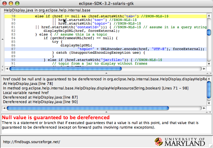
Figure 1: Static code analysis and FindBugs. From http://findbugs.sourceforge.net/.

Static code warnings comment on a range of potential defects such as common programming errors, code styling, in-line comments common programming anti-patterns, style violations, and questionable coding decisions ayewah2008using . Static code warning tools are quite popular. For example the FindBugs static code analysis tool (shown in Figure 1) has been downloaded over a million times.

One issue with static code warnings is that they generate a large number of false positives. Many programmers routinely ignore most of the static code warnings, finding them irrelevant or spurious wang2018there . Such warnings are considered as “unactionable” since programmers never take action on them. Between 35% and 91% of the warnings generated from static analysis tools are known to be unactionable heckman2011systematic . Hence it is prudent to learn to recognize what kinds of warnings programmers usually act upon. With such a classifier, static code warning tools can be made more useful by first pruning away the unactionable warnings.

As shown in this paper, data mining methods can be used to generate very accurate models for this task. This paper searches for 5,675 actionable warnings within a sample of 31,058 static code warnings generated by FindBugs on nine open-source Java projects wang2018there . After the experiment (where we trained on release $i$ then tested on release $i+1$), we built models (using linear SVM) that predicted for actionable warnings with recalls over 87%; false alarms under 7%; and AUC over 97%. These results are a new high watermark in this area of research since they outperform a prior state-of-the-art result (the so-called “golden set” approach reported at ESEM’18 by Wang et al. wang2018there ).

Given that all these learners succeeded so easily, it is appropriate to ask if there is something about this task that is inherently easy. We report that while our data sets have up to 58 raw features, those features can be approximated by less than two underlying dimensions. For such intrinsically simple data, many different kinds of learners can generate useful models with similar performance. Hence, at least for this task, complex methods like deep learners ran far slower and performed no better than much simpler methods. This was somewhat surprising since, to say the least, there are many advocates of deep learning for software analytics (e.g. lin2018sentiment ; guo2017semantically ; chen2019mining ; gu2016deep ; nguyen2017exploring ; choetkiertikul2018deep ; zhao2018deepsim ; white2016deep ).

The rest of this paper is structured as follows. The background to this work is introduced in Section 2. Our methodology is described in Section 3. In Section 3.3 and Section 4, we analyse experiment results. Threats to validity and future work are discussed in Section 5. Our conclusions, drawn in Section 6, will be three-fold:

1. It is possible and effective to augment static code warning tools with a post-processor that prunes away the warnings that programmers will ignore.

2. Before selecting a data mining algorithm, always check the intrinsic dimensionality of the data.

3. After checking the intrinsic dimensionality, match the complexity of the learner to the complexity of the problem.

To facilitate other researchers in this area, all our scripts and data are freely available on-line.

2 Background

2.1 Studying Static Code Warnings

Static code warning tools detect potential static code defects in source code or executable files at the stage of software product development. The distinguishing feature of these tools is that they make their comments without reference to a particular input. Nor do they use feedback from any execution of the code being studied. Examples of these tools include PMD, Checkstyle and the FindBugs tool featured in Figure 1.

As mentioned in the introduction, previous research work shows that 35% to 91% warnings reported as bugs by static warning analysis tools can be ignored by programmers heckman2011systematic . This high false alarm rate is one of the most significant barriers for developers to use these tools thung2015extent ; avgustinov2015tracking ; johnson2013don . Various approaches have been tried to reduce these false alarms including graph theory boogerd2008assessing ; bhattacharya2012graph , statistical models chen2005novel , and ranking schemes kremenek2004correlation . For example, Allier et al. allier2012framework proposed a framework to compare 6 warning ranking algorithms and identified the best algorithms to rank warnings. Similarly, Shen et al. shen2011efindbugs employed a ranking technique to sort true error reports before anything else. Some other works also prioritize warnings by dividing the results into different categories of impact factors liang2010automatic or by analyzing software history kim2007prioritizing .

Table 1: Categories of Wang et al. wang2018there ’s selected features. (8 categories are shown in the left column, and 95 features explored in Wang et al. are shown in the right column with 23 golden features in bold.)

Category	Features
Warning combination	size content for warning type; size context in method, file, package; warning context in method, file, package; warning context for warning type; fix, non-fix change removal rate; defect likelihood for warning pattern; variance of likelihood; defect likelihood for warning type; discretization of defect likelihood; average lifetime for warning type;
Code characteristics	method, file, package size; comment length; comment-code ratio; method, file depth; method callers, callees; methods in file, package; classes in file, package; indentation; complexity;
Warning characteristics	warning pattern, type, priority, rank; warnings in method, file, package;
File history	latest file, package modification; file, package staleness; file age; file creation; deletion revision; developers;
Code analysis	call name, class, parameter signature, return type; new type, new concrete type; operator; field access class, field; catch; field name, type, visibility, is static/final; method visibility, return type, is static/ final/ abstract/ protected; class visibility, is abstract / interfact / array class;
Code history	added, changed, deleted, growth, total, percentage of LOC in file in the past 3 months; added, changed, deleted, growth, total, percentage of LOC in file in the last 25 revisions; added, changed, deleted, growth, total, percentage of LOC in package in the past 3 months; added, changed, deleted, growth, total, percentage of LOC in package in the last 25 revisions;
Warning history	warning modifications; warning open revision; warning lifetime by revision, by time;
File characteristics	file type; file name; package name;

Another approach, and the one taken by this paper, utilizes machine learning algorithms to recognizing which static code warnings that programmers will act upon wang2016automatically ; shivaji2009reducing ; hanam2014finding . For example, when Heckaman et al. applied 15 learning algorithms to 51 features derived from static analysis tool, they achieved recalls of 83-99 % (average across 15 data sets) heckman2009model .

2.2 Wang et al.’s “Golden Set”

The data for this paper comes from a recent study by Wang et al. wang2018there . They conducted a systematic literature review to collect all public available static code features generated by widely-used static code warning tools (116 in total):

• All the values of these collected features were extracted from warning reports generated by FindBugs based on 60 revisions of 12 projects. These projects are selected due to their source code histories spanning for multiple years, sufficient project size and version control system to extract features from wang2018there .

• To ensure that the difference between prior and later revision intervals of a project are adequate to draw solid conclusions, Wang et al. wang2018there set revision intervals for different projects, e.g., 3 months for Lucene and 6 months for Mvn. Each project in this study has at least two-years commit history.

• Six machine learning classifiers were then employed to automatically identify actionable static warning (random forests, decision trees, a boosting algorithm, naive bayes, linear regression, and support vector machines).

• After applying a greedy backward selection algorithm to eliminate noneffective features to the results of those learners, they isolated 23 features as the most useful ones for identifying actionable warnings.

• They called these features the “golden set”; i.e. the features most important for recognizing actionable static code warnings.

To the best of our knowledge, this is the most exhaustive research about static warning characteristics yet published. Therefore, we encourage other researchers in the SE community to continue exploring this data as a standard basis due to the exhaustive feature construction process and the long-spinning code history.

Table 2: Summary of data distribution.

		training set		test set
Dataset	Features	instance counts	actionable ratio(%)	instance counts	actionable ratio(%)
commons	39	725	7	786	5
phoenix	44	2235	18	2389	14
mvn (maven)	47	813	8	818	3
jmeter	49	604	25	613	24
cass (cassandra)	55	2584	15	2601	14
ant	56	1229	19	1115	5
lucence	57	3259	37	3425	34
derby	58	2479	9	2507	5
tomcat	60	1435	28	1441	23

As shown in Table 1, the “golden set” features fall into eight categories. These features are the independent variables used in this study.

To assign dependent labels, we applied the methods of Liang et al. liang2010automatic . They defined a specific warning as actionable if it is closed after the later revision interval. Otherwise, it is labeled as unactionable. Also, after Liang et al., anything labeled a “minor alert” is deleted and ignored.

By analyzing FindBugs output from two consecutive releases of nine software projects, collecting the features of Table 1, and then applying the Liang et al. definitions, we created the data of Table 2. In this table, the “training set” refers to release $i-1$ and the “test set” refers to release $i$. In this study, we only employ two latest releases.

Note that, for any particular data set, the 23 categories of Table 1, can grow to more than 23 features. For example, consider the “return type” feature in the “code analysis” category. This can include numerous return types extracted from a given project, which could be void, int, URL, boolean, string, printStream, file, and date (or a list of any of these periods). Hence, as shown in Table 2, the number of features in our data varied from 39 to 60.

Note also that one way to summarize the results of this paper is that the golden set is an inaccurate, verbose description of the attributes required to detect static code warnings. As shown below, hiding within the 23 feature categories of Table 1, there exist two synthetic dimensions, which can be found via a linear SVM.

2.3 Evaluation Metrics

Wang et al. reported their results in terms of AUC and running time:

• AUC (Area Under the ROC Curve) measures the two-dimensional area under the Receiver Operator Characteristic (ROC) curve witten2016data ; heckman2011systematic . It provides an aggregate and overall evaluation of performance across all possible classification thresholds to overall report the discrimination of a classifier wang2018there . This is a widely adopted measurement in the area of software engineering, especially for imbalanced data liang2010automatic .

• Running time measures the efficiency of the execution of one algorithm. In this paper, we use the running time of one run from the start to the terminal of algorithm execution to compare the efficiency of different models.

Table 3 shows the AUC results achieved by Wang et al. wang2018there . In summary, Wang et al. reported Random Forest as the best learner to identify actionable static warnings.

In the software analytics literature, it is also common to assess learners via recall and false alarms:

• Recall represents the ability of one algorithm to identify instances of positive class or actionable one from the given data set. It denotes the ratio of detected actionable defects in comparison to the total number of actionable defects in the data set generated by static warning tools, like FindBugs.

• False Alarms (pf) measures the instances or warnings generated from static warning tools falsely classified by an algorithm as positive or actionable which are actually negative or unactionable ones. This is an important index used to measure the efficiency of a defect prediction model.

In the following, we will report results for all of these four evaluation measures.

Table 3: %AUC results reported in prior state-of-the-art wang2018there using proposed golden feature set.

Project	Random Forest	Decision Tree	SVM RBF
derby	43	44	50
mvn	45	45	50
lucence	98	98	50
phoenix	71	70	62
cass	70	69	67
jmeter	86	82	50
tomcat	80	64	50
ant	44	44	50
commons	57	56	50
median	70	64	50

2.4 Learning to Recognize Actionable Static Code Warnings

Recall from the above that our data has two classes: actionable and non-actionable. Technically speaking, our task is a binary classification problem. A recent survey by Ghotra et al. ghotra2015revisiting found that for software analytics, the performance of dozens of binary classifications clusters into a handful of groups. Hence, by taking one classifier from each group, it is possible for just a few classifiers to act as representatives for a wide range of commonly used classifiers.

Decision trees quinlan1987generating seek splits to feature ranges that most minimize the diversity of classes within each split. Once the best “splitter” is found, decision tree algorithms recurse on each split.

Random forests breiman1999random take the idea of decision trees one step further. Instead of building one tree, random forests build multiple trees (each time using a small random sample of the rows and columns from the original data). The final conclusion is then computed by a majority vote across all trees in the forest.

Support vector machines cortes1995support take another approach. With a kernel function, the data is mapped into a higher-dimensional space. Then, using a quadratic programming, the algorithm finds the “support vectors” which are the instances closest to the boundary between to distinguish different classes.

2.5 Deep Learning

Since the Ghortra et al. survey ghotra2015revisiting was published in 2015, there has been much recent interest in the application of deep learning (DL) in software engineering. Applications of DL include bug localization huo2019deep , sentiment analysis lin2018sentiment ; guo2017semantically , API mining chen2019mining ; gu2016deep ; nguyen2017exploring , effort estimation for agile development choetkiertikul2018deep , code similarity detection zhao2018deepsim , code clone detection white2016deep , etc.

Deep neural networks are layers of connected units called neurons. A brief mechanism of fully connected DNN model is shown in Figure 2. For this paper, SE artifacts are transferred into vectors and fed into the neural networks as inputs in the input layer. Each neuron in hidden and output layers functions by multiplying its input with the weight of this neuron. Then the product is summed and then passed through a nonlinear transfer function called activation function to yield a variable. It either continuously serves as input to the next layer or final output of the network goh1995back .

Figure 2 illustrates a layered architecture of neurons where inputs at layer $i$ are organized and synthesized as inputs at layer $i+1$ by non-linear transformations mentioned above. It’s known as an automatic feature engineering model which efficiently extracts the non-linear and sophisticated patterns generally observed in the real world, like speech, video, audio. For instance, technology-intensive companies like Google and Facebook are utilizing massive volumes of raw data for commercial data analysis  najafabadi2015deep . Within that layered architecture, only the most important signal from the inputs of layer $i$ will make it through to layer $i+1$. In this way, DL automates “feature engineering” which is the synthesis of important new features using some part or combination of other features. This, in turn, means that predictors can be learned from very complex input signals with multiple features, without requiring manual pre-processing. For example, Lin et al. Lin2017StructuralDD replaced their mostly manual analysis of $10^{4}$ features extracted from a wavelet package with a deep learner that automatically synthesized significant features.

DL trains its networks by running its data repeatedly through networks shown in Figure 2 in multiple “epochs”. Each epoch pushes all the data by batch over the network and the resulting error on the output layer is computed. This repeats until the training error or loss function on the validation set is minimized. Error minimization is done via back propagation (BP). Parameters in DL (including neuron weights), are initialized randomly, and then these parameters of neurons are updated in each epoch of training using error back propagation. Hornik et al. hornik1991approximation have shown that with sufficient hidden neurons, a single hidden layer back-propagation neural network can accurately approximate any continuous function.

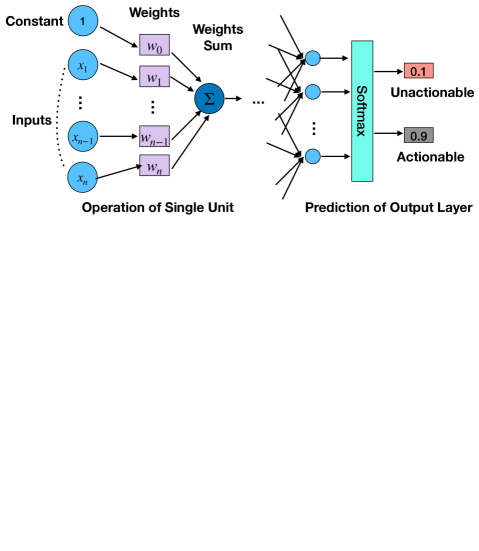
Figure 2: Illustration of DNN Model.

DL training may require hundreds to thousands of epochs in complicated problems. However, overtraining makes the model overfit the training dataset and have poor generalization ability on the test set. Early stopping zhang2016understanding is a commonly used optimizer strategy and regulariser in deep learning, which improves generalization and prevents models from overfitting. It stops training when performance on a validation dataset starts to degrade. We tried to prevent overfitting in our domain via early stopping. The maximum epochs are set as 100, and the patience of early stopping as 3, i.e. stopping training DLs if the performance on the training set is not getting better for continuous three epochs. After running our DLs, we could not improve performance after 8 to 30 epochs. Hence, all the results reported below come from 8 to 30 epochs.

3 Experiments

3.1 Learning Schemes

For this study, the non-DL learners came from SciKit-Learn pedregosa2011scikit while the DL methods came from the Keras package geron2019hands . For the three non-DL learners (Random Forests, Decision Tree, linear Support vector machines), we ran these using their default control settings from SciKit-Learn. As to Deep Learning, we ran three DL schemes. As suggested in the literature review li2018deep , (fully-connected) deep neural network (DNN) and convolutional neural network (CNN) are mostly explored DL models in SE area.

The first scheme is a fully connected deep neural network (DNN). For a description of this method, see Section §2.5. Starting with the defaults from Keras, we configure our DNN model as follows:

• 5 fully connected layers (with 30 neurons for each hidden layer) concatenated by dropout layers in between.

• The activation functions for hidden layers were implemented using the Relu function. Relu represents a rectified linear unit, whose formula is denoted as $f(x)=max(0,x)$. As a universal choice of various activation functions, Relu is known for many merits like fast to compute and converge in practice and its gradients not vanishing when $x>1$ holds or the current neuron is activated li2017convergence . Batch normalization layers are conducted before each activation function to avoid the internal covariate shift (with the distribution changes of parameters in training deep neural networks, the current layer has to constantly readjust to new distributions) ioffe2015batch .

• As said above, actionable warning identification is a binary problem. That is, for any instance $i$ of warnings, its label $y_{i}\in\{0,1\}$, where $0$ denotes this warning is unactionable and $1$ denotes as actionable. Consequently, we use softmax as the activation function for the output of our network in the output layer. Softmax takes the vectors generated from the last hidden layer as inputs and proceeds them by exponentiation operation with a power of $e$ and mapping it into a list of probability distribution of all the label class candidates. For each instance, the list of Softmax vector $[P_{0},P_{1}]$ generated from softmax function always sums to 1, where $P_{0}$ is the probability that this bug is unactionable while $P_{1}$ denoted as actionable.

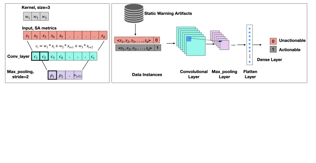
Figure 3: Overview of CNN Model in Static Warning Identification.

Our second scheme is CNN (convolutional neural network) goodfellow2016deep , a widely used DL method which employs weight sharing and pooling schemes. Figure 3 illustrates the overview scheme of applying CNN in static warning analysis. Convolutional layers work with a filter of inputs to build a feature map for repeated times, whose principle is looking for correlation between filter and input feature matrix. And max pooling layers reduce spatial size of features by selecting maximum value to represent a feature window. With weight sharing of filters and max pooling, CNNs can greatly reduces the parameters required in training phase.

DNN_weighted is our third DL scheme whose main structure is the same as DNN mentioned above but also use a weighted strategy. Table 2 shows that many of our data sets have unbalanced class distributions where our target class (actionable warnings) is very under-represented (often less than 20%). To address this data imbalance problem, we re-weight the minority class, actionable class. Specifically, we use the reciprocal of the ratio for class 0 and 1 to weight the loss function during the training phase. For instance, the ratio of actionable samples in training set is 0.25, the weighting scheme sets the weight of actionable (minority) as 4, and unactionable (majority) as 1 to balance the significance of training loss for two classes in the training process. Note that we used this reweighting scheme rather than some alternative method (e.g. duplicate instances of minority class) since reusing many copies of one instance in the training set causes extra computational cost shalev2014understanding .

3.2 Statistical Tests

To select “best” learning methods, the advice of Rosenthal et al. rosenthal1994parametric is taken in this paper. Specifically, given that all our numbers are with 0..1, then experiment results are not prone to extreme outlier effects via statistical tests. Such extreme outliers are indicators for long-tail effects which, in turn suggest that it might be better to use non-parametric methods. This is not ideal since non-parametric tests have less statistical power than parametric ones.

Rosenthal et al. discuss different parametric methods for asserting that one result is with some small effect of another (i.e. it is “close to”). They list dozens of effect size tests that divide into two groups: the $r$ group that is based on the Pearson correlation coefficient; or the $d$ family that is based on absolute differences normalized by (e.g.) the size of the standard deviation. Rosenthal et al. comment that “none is intrinsically better than the other”. The most direct method is utilized in our paper. Using a $d$ family method, it can be concluded that one distribution is the same as another if their mean value differs by less than Cohen’s delta ($d$*standard deviation). Note that $d$ is computed separately for each different evaluation measure (recall, false alarm, AUC).

To visualize that “close to” analysis, in all our results:

• Any cell that is within $d$ of the best value will be highlighted in gray. All gray cells are observed as “winners” and all the other cells are “losers”.

• For recall and AUC, the “best” cells have “highest value” since the optimization goal is to maximize these values.

• For false alarm, the “best” cells have “lowest value” since false alarms is to be minimized.

As to what value of $d$ to use in this analysis, we take the advice of a widely cited paper by Sawilowsky sawilowsky2009new (this 2009 paper has 1100 citations). That paper asserts that “small” and “medium” effects can be measured using $d=0.2$ and $d=0.5$ (respectively). Splitting the difference, we will analyze this data looking for differences larger than $d=(0.5+0.2)/2=0.35$.

3.3 Results

In the text of Empirical AI, Cohen advises that any method uses a random number generator must be run multiple times, to allow for any effects introduced by the random number seed. For deterministic models, the same output is always produced for the same sequence of given a particular input. To dispel the bias between deterministic and non-deterministic models and eliminate the bias of uncertainty:

• Ten times, we shuffled the training and test data into some random order.

• Each time, divide the test data into five bins, taking care to implement stratified sampling; i.e. ensuring that the class distribution of the whole data is replicated within each bin. In this way, the distributions of training and testing set are kept unchanged, as shown in Table 2.

• For each 20% test bins, learn a model using 100% of the training set.

Table 4: Summary results of recall, false alarm and AUC on nine datasets. Cells in gray denote the “best” results for each row, where “best” means within $d$ difference to the best value (and $d$ is calculated as per §3.2.)

Project DNN weighted CNN DNN Random Forest Decision Tree SVM linear derby 96.6% 96.9% 94.0% 92.0% 94.8% 97.8% mvn 97.6% 95.0% 92.0% 78.9% 94.7% 97.0% lucence 95.3% 98.1% 91.3% 96.8% 96.6% 87.1% Recall phoenix 95.2% 93.0% 89.3% 88.7% 86.8% 96.1% cass 81.3% 98.8% 68.1% 76.8% 75.7% 90.3% (d = 3%) jmeter 94.3% 93.9% 89.2% 96.9% 92.7% 93.3% tomcat 98.0% 95.0% 96.4% 91.8% 87.6% 98.2% ant 91.1% 93.1% 84.1% 78.7% 87.0% 95.0% commons 81.1% 97.8% 73.3% 66.7% 92.0% 99.5% derby 1.2% 10.8% 0.5% 0.3% 0.5% 1.3% mvn 1.4% 6.8% 0.4% 0.5% 0.4% 1.2% lucence 5.9% 5.8% 3.2% 1.4% 3.2% 6.9% False phoenix 3.0% 8.7% 1.4% 1.3% 0.7% 3.5% Alarm cass 1.2% 7.0% 0.4% 2.5% 1.3% 1.4% jmeter 3.1% 48.6% 1.4% 1.3% 0.4% 2.1% tomcat 2.1% 8.8% 1.3% 0.4% 4.3% 3.2% (d=2%) ant 0.5% 6.7% 0.5% 0.4% 0.5% 0.5% commons 3.1% 8.6% 1.4% 0.2% 1.4% 5.8% derby 99.7% 97.2% 99.6% 99.7% 97.1% 99.5% mvn 99.9% 99.1% 99.9% 99.6% 96.8% 99.6% lucence 98.7% 98.7% 98.8% 99.6% 96.6% 97.3% AUC phoenix 98.5% 97.8% 98.8% 98.6% 92.7% 98.8% cass 97.0% 98.0% 96.9% 98.6% 88.0% 99.7% (d=1%) jmeter 98.7% 82.3% 97.7% 99.7% 95.9% 98.8% tomcat 100.0% 98.3% 99.7% 99.6% 92.1% 99.6% ant 98.9% 97.3% 97.7% 98.7% 93.3% 99.7% commons 96.0% 99.2% 97.7% 98.7% 96.1% 99.0%

Table 5: Comparing median results and IQR of recall, false alarm and AUC. Cells in gray denote the “best” median results for each row, where “best” means within $d$ difference to the best value in each row (and $d$ is calculated as per §3.2.)

metrics measures DNN weighted CNN DNN Random Forest Decision Tree SVM linear recall median 95.2% 95.1% 89.3% 88.7% 92.0% 96.1% (d=1%) IQR 5.4% 3.9% 8.0% 13.3% 7.7% 4.5% false alarm median 2.1% 8.6% 1.3% 0.5% 0.7% 2.1% (d=1%) IQR 1.9% 2.0% 0.9% 0.9% 0.9% 2.2% AUC median 98.7% 98.0% 98.8% 99.5% 95.9% 99.5% (d=0%) IQR 1.2% 1.5% 1.9% 0.9% 3.9% 0.8%

Table 6: Comparing results of running time sorted by size of datasets in a descending order on nine projects from six learners.

Project DNN weighted CNN DNN Random Forest Decision Tree SVM linear lucence 188.3 233.1 201.0 3.9 3.2 25.8 cass 172.5 368.1 195.6 2.4 2.5 7.9 derby 145.0 351.7 156.5 2.7 2.3 7.7 phoenix 134.6 293.6 148.2 2.1 2.1 6.1 Runtime(/s) tomcat 119.2 280.6 112.5 1.8 1.4 3.4 ant 110.6 259.4 123.5 1.8 1.3 2.4 mvn 70.4 114.6 73.7 1.9 0.9 1.6 commons 86.5 124.5 96.1 1.5 0.7 1.1 jmeter 57.0 110.8 60.8 1.5 0.8 1.3 Average 120.5 237.4 129.8 2.2 1.7 6.4

Table 4 shows the results of our experiment rig. The gray cells show results that are either (a) the best values or (b) are as good as the best. Counting the winning gray cells and the other white cells, we can see that:

• Linear SVM are often preferred (lower false alarms, higher recall and AUC).

• The tree learners have many white cells; i.e. they perform worse than best.

• The deep learners (DNN weighted, CNN, DNN) are often gray– but not as often as SVM linear.

Hence we say that linear SVM has the best all-around performance.

Another reason to prefer SVMs over deep learners is shown in Table 6. This table shows the runtimes of our different learners: deep learners were very much slower than the other learners (at least 20 times faster).

Note that, compared with Table 3, our AUC results shown in Table 4 and Table 5 are much better than Wang et al.’s, which we explain as follows. Firstly, the default parameters in Weka (used by Wang et al.) are different to those used in SciKit-Learn  (the tool employed in our paper).

Secondly, we use a different SVM to Wang et al. In Table 4, Random Forest performs best in baseline models from the perspective of AUC which is consistent with Wang et al. While SVM result indicates significant difference due to different choices of kernels. (We also conducted an experiment on SVM with RBF kernel and got median AUC as 0.5.)

In summary, we can endorse the use of linear SVM in this domain, but not deep learners or tree learners.

4 Why Such Similar Performance?

A question raised by the above results is why do different learners perform so similarly on all these data sets. Accordingly, this section explores that issue.

We will argue that the above results illustrates Vandekerckhove et al. Principle of Parsimony. They warn that unnecessary sophisticated models can damage the generalization capability of the classifiers vandekerckhove2015model . This principle is a strategy that warns against overfitting (and is a fundamental principle of model selection). It suggests that simpler models are preferred than complex ones if those models obtain similar performance.

A convincing demonstration that Principle of Parsimony has two parts:

1. We must show some damage to the generalization capability of a complex classifier. For example, in the above, we found that even though deep learner’s automatic feature engineering may account for irrelevant particulars (like noise in the data), they did not perform better than linear SVM.

2. We must also show that the data set has only very few dimensions; i.e. a complex learner is exploring an inherently simple set of data. In the rest of this section, using an intrinsic dimensionality calculator, we will show that the intrinsic dimensionality of our static warning data sets is never more than two and usually is less.

To say all that another way, since the problem explored in our study is inherently low dimensional, it is hardly surprising that the sophistication of deep learning was not useful in this domain.

4.1 What is “Intrinsic Dimensionality”?

Levina et al. levina2005maximum comment that the reason any data mining method works for high dimensions is that data embedded in high-dimensional format actually can be converted into a more compressed space without major information loss. A traditional way to compute these intrinsic dimensions is PCA (Principal Component Analysis). But Levina et al. caution that, as data in the real-world becomes increasingly sophisticated and non-linearly decomposable, PCA methods tend to overestimate the dimensions of a data set levina2005maximum .

Instead, Levina et al. propose a fractal-based method for calculating intrinsic dimensionality (and that method is now a standard technique in other fields such as astrophysics). The intrinsic dimension of a data set with N items is found by computing the number of items found at distance within radius r (where r is the distance between two configurations) while varying r. This measures the intrinsic dimensionality since:

• If the items spread out in only one $r=1$ dimensions, then we will only find linearly more items as $r$ increases.

• But the items spread out in, say, $r>1$ dimensions, then we will find polynomially more items as $r$ increases.

As shown in Equation 1, Levina et al. normalize the number of items found according to the number of $N$ items being compared. They recommend reporting the number of intrinsic dimensions as the maximum value of the slope between $\mathit{ln(r)}$ vs the $\mathit{ln}(C(r))$ value computed as follows. Note Equation 1 use the L1-norm to calculate distance rather than the Euclidean L2-norm. As seen in Table 2, our raw data has up to 60 dimensions. Courtney et al. Aggarwal01 advise that for such high dimensional data, L1 performs better than L2.

$$C(r)=\frac{2}{N(N-1)}\sum_{i=1}^{N}\sum_{j=i+1}^{N}I(||x_{i},x_{j}||<r)$$ (1)

$$where:I(||x_{i},x_{j}||<r)=\left\{\begin{aligned} 1,||x_{i},x_{j}||<r\\ 0,||x_{i},x_{j}||\geq r\end{aligned}\right.$$

For example, in Figure 4, the intrinsic dimensionality of blue curve is 1.6 approximated by the maximum slope which is the orange line.

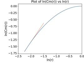
Figure 4: Intrinsic dimensionality is the maximum slope of the smoothed blue curve of $\mathit{ln(r)}$ vs $\mathit{ln}(C(r))$ (see the orange line).

 Import data from Testdata.py  Input: $\mathit{sample}\_\mathit{num}=n,\mathit{sample}\_\mathit{dim}=d$  $Rs_{\mathit{log}}=\mathit{start:end:step}$   $Rs=\mathit{np}.\mathit{exp}(Rs_{\mathit{log}})$  for $R$ in $Rs$ do     # Calculated by L1 Distance     $I=0$     # count for pairwise samples within R     for $i,j$ in $\mathit{combinations}(\mathit{data},2)$ do        $d=\mathit{distance}(i,j)$        # L1 distance        if $d<R$ then           $I\leftarrow I+1$        end if     end for     $Cr=2*I/n*(n-1)$  end for  $Crs.\mathit{append}(Cr)$  for $i$ in $\mathit{step}$ do     $\mathit{gradient}=(Crs[i]-Crs[i-1])/(R[i]-R[i-1])$     $GR.\mathit{append}(\mathit{gradient})$  end for  $\mathit{Smooth}(GR)$  # smooth the curve  $\mathit{intrinsicD}\leftarrow\mathit{max}(GR)$  # Estimate the intrinsic dimensionality

Algorithm 1 Intrinsic Dimension by Box-counting Method

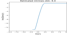
(a) d=5, s=1000

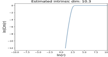
(b) d=10, s=1000

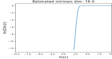
(c) d=20, s=1000

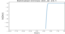
(d) d=40, s=1000

Figure 5: Algorithm 1 works well for up to 20 intrinsic dimensions. To show that, we randomly filled 1000 rows of tables of data with $d$ columns with random variables $0\leq X\leq 1$. Algorithm 1 came close to the actual value of $d$ for $d<20$. Above that point, the algorithm, seems to underestimate the number of columns– an effect we attribute to the “shotgun correlation effect” reported by Courtney et al. courtney93 in 1993. They reported that, due to randomly generated spurious correlations, the correlation between $d$ random variables will increase with $d$. Hence it is not surprising that in the (e.g.) $d=40$ plot of this figure, we find less than 40 dimensions.

Algorithm 1 shows the intrinsic dimensionality calculator used in this paper. Note that this calculator uses Equation 1 with an L1-norm. Figure 5 displays a verification study which shows that this algorithm works well for up to 20 intrinsic dimensions.

4.2 Intrinsic Dimensionality and Static Code Warnings

Table 7 shows the results of applying our intrinsic dimensionality calculator to the static code warning data. In that table, we observe that:

• The size of the data set is not associated with intrinsic dimensionality. Evidence: our largest data set (Lucene) has the lowest intrinsic dimensionality.

• The intrinsic dimensionality of our data is very low (median value of less than one, never more than two), which is latent dimensionality instead of subsetting from original features.

This paper is not the first to suggest that several SE data sets are low dimensional in data. Menzies et al. also review a range of strange SE results, all of which indicate that the effective number of dimensions of SE data is very low menzies07 . Also, Agrawal et al. agrawal2019dodge argued that dimensionality of the space of performance scores generated from some software effectively divides into just a few dozen regions– which is a claim we could restate as that space is effectively low dimensional. Further, Hindle et al. Hindle:2016 made an analogous argument that:

“Programming languages, in theory, are complex, flexible and powerful, but the programs that real people actually write are mostly simple and rather repetitive, and thus they have usefully predictable statistical properties that can be captured in statistical language models and leveraged for software engineering tasks.”

That said, Hindle, Agrawal, and Menzies et al. only show that there can be a benefit in exploring SE data with tools that exploit low dimensionality. None of that work makes the point made in this paper, that for SE data it can be harmful to explore low dimensional SE data with tools designed for synthesizing models from high dimensional spaces (such a deep learners).

Table 7: Summary of dimensionality of nine datasets. Calculated using Equation 1.

Dataset	original dimensionality	intrinsic dimensionality	instance counts
lucence	57	0.15	3259
phoenix	44	0.62	2235
tomcat	60	0.73	1435
derby	58	0.78	2479
Ant	56	0.82	1229
commons	39	1.04	725
mvn	47	1.10	813
jmeter	49	1.54	604
cass	55	1.94	2584

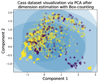
(a) Cass: Estimated Dim = 1.94, visualized in 2-D space via PCA

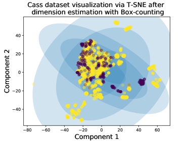
(b) Cass: Estimated Dim = 1.94, visualized in 2-D space via T-SNE

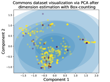
(c) Commons: Estimated Dim = 1.04, visualized in 2-D space via PCA

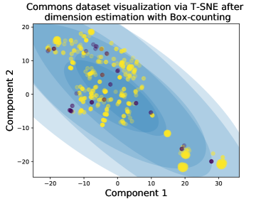
(d) Commons: Estimated Dim = 1.04, visualized in 2-D space via T-SNE

Figure 6: In this figure, we tried visualizing the underlying intrinsic dimensions of our data using PCA and T-SNE. In summary, those tools were not useful for finding those dimensions. We say that since the clusters shown here do not separate the actionable and unactionable warnings. Results here come from GMM (Gaussian mixture clustering). This algorithm is known to be more robust than K-means due to its capability to incorporate the uncertainty of the sample labels rasmussen1999infinite . In these figures: (a) the x-y plots from the first two components found by PCA and T-SNE; (b) darker ellipses are regions closer to the cluster centroids; (c) actionable warnings are shown in purple dots; (d) unactionable warnings are shown in yellow. Data from these figures come from cass and commons. Results from other data sets are just as uninformative. In future work, it could be useful to return to this goal of trying to visualize the underlying intrinsic dimensions, perhaps with other clustering tools.

Lastly, we report on a failed attempt to visualize our data. Recall from the above that Levina et al. caution against the use PCA. Consistent with that warning, we found PCA plots to be uninformative. We further incorporate a nonlinear visualization tool (T-SNE maaten2008visualizing ), a widely used probability-based model to depict our data set. As shown in Figure 6, those tools were not useful for separating out our classes. In future work, it could be useful to return to this goal (of trying to visualize the underlying intrinsic dimensions), perhaps with other clustering tools.

4.3 Summary

After applying Algorithm 1 to our data, we can assert that static code warning is inherently a low dimensional problem. Specifically, our data sets can be characterized with less than two dimensions as reported in Table 7. Hence, we believe that the reason deep learning performs so similarly or even worst than conventional learners for static code warnings is that it is a very big hammer being applied to a very small nail.

5 Discussion

5.1 Threats to Validity

Before discussing threats to validity, we make the meta-comment that induction is not a certain inference since (e.g.) just because the sun has risen every day since the birth of this planet, we cannot say with 100% certainty that it will rise tomorrow. Project data differs from project to project and just because we found that past data generated a clear signal on what was an actionable code warning (see Table 4), there is no guarantee that such a signal will be found in future data. Hence, any data mining paper will raise issues of (e.g.) sampling bias and measurement bias. 
     To address this concern, we assert that data mining researchers need to express their conclusions in a refutable manner. To that end, we take care to draw our conclusions from data and tools that are free to download and which are distributed under open source licenses that enable their widespread use.

Sampling bias. In terms of sampling bias, our first comment is that all our conclusions are based on the data explored in the above experiments. For future work, we need to repeat this analysis using different data sets. Our second comment is while we depreciate deep learning, that warning only applies to low dimensional data. Deep learning is very useful for very high dimensional problems; e.g. vision systems in autonomous cars.

For this specific research task, we explore the static warning data set collected by a prior EMSE paper. Wang’s study reduces our sampling bias issue (due to the thoroughness of that analysis). That said, sample bias threatens any paper on analytics (not just this one) since conclusions that hold for one project may not hold for any other. No paper can explore all data sets – the best we can do (and we have done) is carefully documenting our methods and placing our tools on a repository that others can access (so the community can easily apply our methods to their data).

Measurement bias: To evaluate the efficiency of our learners, we employ three commonly used measurement metrics in SE area: recall, false alarm, and AUC. Several prior research works have demonstrated the necessity and effectiveness of these measurements yu2018finding ; wang2018there . For the static warning analysis task, the major goal is to identify the true positives, so recall and false-positive rate are adequate measurements. Also, AUC indicates the overall performance of a classifier. There exist many other metrics widely adopted by SE community, like F1 score, G measure and so forth. For the same research question, different conclusions may be drawn by using various evaluation metrics. In future work, we would use other evaluation metrics to have a more comprehensive analysis.

Parameter bias: This paper used the default settings for our learners (exception: we adjusted the number of epochs used in our deep learners). Recent work Tantithamthavorn16 ; agrawal2018better ; agrawal2019dodge has shown that these defaults can be improved via hyperparameter optimization (i.e., learners applied to learners to learn better settings for the control parameters). In this study, we found that even with the default parameters we could outperform deep learning and prior state-of-the-art results wang2018there . Hence, we leave hyperparameter optimization for future work.

Learner bias. One of the most important threats to validity is learner bias, since there is no theoretical reason that any learner outperforms others in all test cases. Wolpert et al. wolpert1997no and Tu et al. Tu18Tuning proposed that no learner necessarily works better than others for all possible optimization problems. Moreover, there also exist many other deep models developed in deep learning revolution. Different models show significant advantages in different tasks. For instance, LSTM is utilized in Google Translate to translate between more than 100 languages efficiently, while CNN is widely used in tasks of analyzing visual imagery. In this case, researchers may find other deep neural networks work better on SE tasks. For future work, we need to repeat this analysis using different learners.

5.2 Future Work

In future work, it would be interesting to do more comparative studies of SE data using deep learning versus other kinds of learners. Those studies should pay particular attention to the issue raised here; i.e. does DL match the complexity of datasets in other SE areas? Also, we can exploit the deep learning effect described above to generate a new generation of better learners. In the literature, non-linear mapping methods that can project complex features into lower dimension space are widely explored in the areas of statistics and computer vision krizhevsky2012imagenet . Such feature reduction can significantly save computational overhead brought by complex algorithms such as DNN models. Therefore, the implementation of non-linear feature mapping might dispel the concern of SE researchers caused by the overwhelming running cost of deep learning models on big datasets (as well as contribute to the promotion of deep learning in SE area). A comprehensive implementation of non-linear feature mapping is left to future work.

Also, another avenue for future work would be to drill down into specific warnings types for static warnings generated by Findbugs. As illustrated in prior literature khalid2015examining , more than 400 possible types of warnings identified by Findbugs can be categorized into eight groups (bad practice, correctness, internationalization, malicious code vulnerability, multi-threaded correctness, performance, security, and dodgy code). These warnings can be assigned a priority (e.g., low, medium, and high) which indicates how confident this warning is an actionable one or true positive. We think it would be insightful to check how specific types of warnings are essential for the software community because prior literature indicated specific types of warnings (e.g., bad-practice, internationalization and, performance) had significantly higher densities in low-rated apps than high-rated ones. Such a more “fine-grained” investigation could provide a very meaningful guideline for SE researchers.

In addition, we plan to apply these static analysis methods to other kinds of data. Currently, we are in open discussions with the Linux developers about applying these methods to their domain for the particular task of reducing the number of false alarms generated by security static code analyzers. This work is in progress and, to date, we have nothing definitive to report.

Finally, in Figure 6 we show failed experiments in trying to visualize the underlying intrinsic dimensions. In future work, it would be useful to return to this goal, perhaps with other clustering tools.

6 Conclusion

Static code analysis tools produce many false positives which many programmers ignore. Such tools can be augmented with data mining algorithms to prune away the spurious reports, leaving behind just the warnings that cause programmers to take action to change their code. As seen by the above results, such data miners can be remarkably effective (and exhibit very low false alarm rates, very high AUC results, and respectably high recall results).

In this paper, we perform an empirical experiment to apply tree learners, linear SVM, and deep learning (with early stopping) to predicting actionable static warning analysis tasks on nine software projects. We find deep learners mismatch the complexity of our static warning datasets with high running cost. Using a dimension reduction algorithm, our static warning datasets are reported as inherently low dimensional. As suggested by Principle of Parsimony, it is detrimental to employ sophisticated models (like deep learning) on data that is inherently low dimensional (like the data explored here). Hence, we endorse the use of linear SVM for predicting which static code warnings are actionable.

To end, we note the irony of this paper. In this paper, we turned to intrinsic dimensionality after exploring particular data set– which is the opposite for what we are recommending for future practice. For future work in software analytics, we suggest that analysts match the complexity of their analysis tools to the underlying complexity of their research problem. Specifically, we strongly urge the SE community to compute the dimensionality of their data, then use those results to select an appropriate analysis algorithm.

7 Acknowledgment

This work was partially funded by an NSF award #1703487.

References

- (1) Aggarwal, C.C., Hinneburg, A., Keim, D.A.: On the surprising behavior of distance metrics in high dimensional spaces. In: Proceedings of the 8th International Conference on Database Theory, ICDT ’01, p. 420–434. Springer-Verlag, Berlin, Heidelberg (2001)
- (2) Agrawal, A., Fu, W., Chen, D., Shen, X., Menzies, T.: How to ”dodge” complex software analytics. Preprint, IEEE Transactions on Software Engineering (2019). Available on-line at http://arxiv.org/abs/1902.01838
- (3) Agrawal, A., Menzies, T.: Is better data better than better data miners?: on the benefits of tuning smote for defect prediction. In: International Conference on Software Engineering (2018)
- (4) Allier, S., Anquetil, N., Hora, A., Ducasse, S.: A framework to compare alert ranking algorithms. In: 2012 19th Working Conference on Reverse Engineering, pp. 277–285. IEEE (2012)
- (5) Avgustinov, P., Baars, A.I., Henriksen, A.S., Lavender, G., Menzel, G., de Moor, O., Schäfer, M., Tibble, J.: Tracking static analysis violations over time to capture developer characteristics. In: Proceedings of the 37th International Conference on Software Engineering-Volume 1, pp. 437–447. IEEE Press (2015)
- (6) Ayewah, N., Pugh, W., Hovemeyer, D., Morgenthaler, J.D., Penix, J.: Using static analysis to find bugs. IEEE software 25(5), 22–29 (2008)
- (7) Bhattacharya, P., Iliofotou, M., Neamtiu, I., Faloutsos, M.: Graph-based analysis and prediction for software evolution. In: 2012 34th International Conference on Software Engineering (ICSE), pp. 419–429. IEEE (2012)
- (8) Boogerd, C., Moonen, L.: Assessing the value of coding standards: An empirical study. In: 2008 IEEE International Conference on Software Maintenance, pp. 277–286. IEEE (2008)
- (9) Breiman, L.: Random forests. UC Berkeley TR567 (1999)
- (10) Chen, C., Xing, Z., Liu, Y., Ong, K.L.X.: Mining likely analogical apis across third-party libraries via large-scale unsupervised api semantics embedding. IEEE Transactions on Software Engineering (2019)
- (11) Chen, W.C., Tseng, S.S., Wang, C.Y.: A novel manufacturing defect detection method using association rule mining techniques. Expert systems with applications 29(4), 807–815 (2005)
- (12) Choetkiertikul, M., Dam, H.K., Tran, T., Pham, T.T.M., Ghose, A., Menzies, T.: A deep learning model for estimating story points. IEEE Transactions on Software Engineering (2018)
- (13) Cortes, C., Vapnik, V.: Support-vector networks. Machine learning 20(3), 273–297 (1995)
- (14) Courtney, R., Gustafson, D.: Shotgun correlations in software measures. Software Engineering Journal 8 (1993)
- (15) Géron, A.: Hands-On Machine Learning with Scikit-Learn, Keras, and TensorFlow: Concepts, Tools, and Techniques to Build Intelligent Systems. O’Reilly Media (2019)
- (16) Ghotra, B., McIntosh, S., Hassan, A.E.: Revisiting the impact of classification techniques on the performance of defect prediction models. In: Proceedings of the 37th International Conference on Software Engineering-Volume 1, pp. 789–800. IEEE Press (2015)
- (17) Goh, A.T.: Back-propagation neural networks for modeling complex systems. Artificial Intelligence in Engineering 9(3), 143–151 (1995)
- (18) Goodfellow, I., Bengio, Y., Courville, A.: Deep learning. MIT press (2016)
- (19) Gu, X., Zhang, H., Zhang, D., Kim, S.: Deep api learning. In: Proceedings of the 2016 24th ACM SIGSOFT International Symposium on Foundations of Software Engineering, pp. 631–642. ACM (2016)
- (20) Guo, J., Cheng, J., Cleland-Huang, J.: Semantically enhanced software traceability using deep learning techniques. In: 2017 IEEE/ACM 39th International Conference on Software Engineering (ICSE), pp. 3–14. IEEE (2017)
- (21) Hanam, Q., Tan, L., Holmes, R., Lam, P.: Finding patterns in static analysis alerts: improving actionable alert ranking. In: Proceedings of the 11th Working Conference on Mining Software Repositories, pp. 152–161. ACM (2014)
- (22) Heckman, S., Williams, L.: A model building process for identifying actionable static analysis alerts. In: 2009 International Conference on Software Testing Verification and Validation, pp. 161–170. IEEE (2009)
- (23) Heckman, S., Williams, L.: A systematic literature review of actionable alert identification techniques for automated static code analysis. Information and Software Technology 53(4), 363–387 (2011)
- (24) Hindle, A., Barr, E.T., Gabel, M., Su, Z., Devanbu, P.: On the naturalness of software. Commun. ACM 59(5), 122–131 (2016). DOI 10.1145/2902362. URL http://doi.acm.org/10.1145/2902362
- (25) Hornik, K.: Approximation capabilities of multilayer feedforward networks. Neural networks 4(2), 251–257 (1991)
- (26) Huo, X., Thung, F., Li, M., Lo, D., Shi, S.T.: Deep transfer bug localization. IEEE Transactions on Software Engineering (2019)
- (27) Ioffe, S., Szegedy, C.: Batch normalization: Accelerating deep network training by reducing internal covariate shift. arXiv preprint arXiv:1502.03167 (2015)
- (28) Johnson, B., Song, Y., Murphy-Hill, E., Bowdidge, R.: Why don’t software developers use static analysis tools to find bugs? In: Proceedings of the 2013 International Conference on Software Engineering, pp. 672–681. IEEE Press (2013)
- (29) Khalid, H., Nagappan, M., Hassan, A.E.: Examining the relationship between findbugs warnings and app ratings. Ieee Software 33(4), 34–39 (2015)
- (30) Kim, S., Ernst, M.D.: Prioritizing warning categories by analyzing software history. In: Proceedings of the Fourth International Workshop on Mining Software Repositories, p. 27. IEEE Computer Society (2007)
- (31) Kremenek, T., Ashcraft, K., Yang, J., Engler, D.: Correlation exploitation in error ranking. In: ACM SIGSOFT Software Engineering Notes, vol. 29, pp. 83–93. ACM (2004)
- (32) Krizhevsky, A., Sutskever, I., Hinton, G.E.: Imagenet classification with deep convolutional neural networks. In: Advances in neural information processing systems, pp. 1097–1105 (2012)
- (33) Levina, E., Bickel, P.J.: Maximum likelihood estimation of intrinsic dimension. In: Advances in neural information processing systems, pp. 777–784 (2005)
- (34) Li, X., Jiang, H., Ren, Z., Li, G., Zhang, J.: Deep learning in software engineering. arXiv preprint arXiv:1805.04825 (2018)
- (35) Li, Y., Yuan, Y.: Convergence analysis of two-layer neural networks with relu activation. In: Advances in neural information processing systems, pp. 597–607 (2017)
- (36) Liang, G., Wu, L., Wu, Q., Wang, Q., Xie, T., Mei, H.: Automatic construction of an effective training set for prioritizing static analysis warnings. In: Proceedings of the IEEE/ACM international conference on Automated software engineering, pp. 93–102. ACM (2010)
- (37) Lin, B., Zampetti, F., Bavota, G., Di Penta, M., Lanza, M., Oliveto, R.: Sentiment analysis for software engineering: How far can we go? In: 2018 IEEE/ACM 40th International Conference on Software Engineering (ICSE), pp. 94–104. IEEE (2018)
- (38) Lin, Y.Z., Nie, Z.H., Ma, H.W.: Structural damage detection with automatic feature-extraction through deep learning. Comput. Aided Civ. Infrastructure Eng. 32, 1025–1046 (2017)
- (39) Maaten, L.v.d., Hinton, G.: Visualizing data using t-sne. Journal of machine learning research 9(Nov), 2579–2605 (2008)
- (40) Menzies, T., Owen, D., Richardson, J.: The strangest thing about software. Computer 40(1), 54–60 (2007). DOI 10.1109/MC.2007.37. URL https://doi.org/10.1109/MC.2007.37
- (41) Najafabadi, M.M., Villanustre, F., Khoshgoftaar, T.M., Seliya, N., Wald, R., Muharemagic, E.: Deep learning applications and challenges in big data analytics. Journal of Big Data 2(1), 1 (2015)
- (42) Nguyen, T.D., Nguyen, A.T., Phan, H.D., Nguyen, T.N.: Exploring api embedding for api usages and applications. In: 2017 IEEE/ACM 39th International Conference on Software Engineering (ICSE), pp. 438–449. IEEE (2017)
- (43) Pedregosa, F., Varoquaux, G., Gramfort, A., Michel, V., Thirion, B., Grisel, O., Blondel, M., Prettenhofer, P., Weiss, R., Dubourg, V., et al.: Scikit-learn: Machine learning in python. Journal of machine learning research (2011)
- (44) Quinlan, J.R.: Generating production rules from decision trees. In: ijcai, vol. 87, pp. 304–307. Citeseer (1987)
- (45) Rasmussen, C.: The infinite gaussian mixture model. Advances in neural information processing systems 12, 554–560 (1999)
- (46) Rosenthal, R., Cooper, H., Hedges, L.: Parametric measures of effect size. The handbook of research synthesis 621(2), 231–244 (1994)
- (47) Sawilowsky, S.S.: New effect size rules of thumb. Journal of Modern Applied Statistical Methods 8(2), 26 (2009)
- (48) Shalev-Shwartz, S., Ben-David, S.: Understanding machine learning: From theory to algorithms. Cambridge university press (2014)
- (49) Shen, H., Fang, J., Zhao, J.: Efindbugs: Effective error ranking for findbugs. In: 2011 Fourth IEEE International Conference on Software Testing, Verification and Validation, pp. 299–308. IEEE (2011)
- (50) Shivaji, S., Whitehead Jr, E.J., Akella, R., Kim, S.: Reducing features to improve bug prediction. In: 2009 IEEE/ACM International Conference on Automated Software Engineering, pp. 600–604. IEEE (2009)
- (51) Tantithamthavorn, C., McIntosh, S., Hassan, A.E., Matsumoto, K.: Automated parameter optimization of classification techniques for defect prediction models. In: ICSE’16, pp. 321–332 (2016). DOI 10.1145/2884781.2884857
- (52) Thung, F., Lo, D., Jiang, L., Rahman, F., Devanbu, P.T., et al.: To what extent could we detect field defects? an extended empirical study of false negatives in static bug-finding tools. Automated Software Engineering 22(4), 561–602 (2015)
- (53) Tu, H., Nair, V.: While tuning is good, no tuner is best. In: FSE SWAN (2018)
- (54) Vandekerckhove, J., Matzke, D., Wagenmakers, E.J., et al.: Model comparison and the principle of parsimony. Oxford handbook of computational and mathematical psychology pp. 300–319 (2015)
- (55) Wang, J., Wang, S., Wang, Q.: Is there a golden feature set for static warning identification?: an experimental evaluation. In: Proceedings of the 12th ACM/IEEE International Symposium on Empirical Software Engineering and Measurement, p. 17. ACM (2018)
- (56) Wang, S., Liu, T., Tan, L.: Automatically learning semantic features for defect prediction. In: 2016 IEEE/ACM 38th International Conference on Software Engineering (ICSE), pp. 297–308. IEEE (2016)
- (57) White, M., Tufano, M., Vendome, C., Poshyvanyk, D.: Deep learning code fragments for code clone detection. In: Proceedings of the 31st IEEE/ACM International Conference on Automated Software Engineering, pp. 87–98. ACM (2016)
- (58) Witten, I.H., Frank, E., Hall, M.A., Pal, C.J.: Data Mining: Practical machine learning tools and techniques. Morgan Kaufmann (2016)
- (59) Wolpert, D.H., Macready, W.G., et al.: No free lunch theorems for optimization. IEEE transactions on evolutionary computation 1(1), 67–82 (1997)
- (60) Yu, Z., Kraft, N.A., Menzies, T.: Finding better active learners for faster literature reviews. Empirical Software Engineering 23(6), 3161–3186 (2018)
- (61) Zhang, C., Bengio, S., Hardt, M., Recht, B., Vinyals, O.: Understanding deep learning requires rethinking generalization. arXiv preprint arXiv:1611.03530 (2016)
- (62) Zhao, G., Huang, J.: Deepsim: deep learning code functional similarity. In: Proceedings of the 2018 26th ACM Joint Meeting on European Software Engineering Conference and Symposium on the Foundations of Software Engineering, pp. 141–151. ACM (2018)