Fast Enhancement for Non-Uniform Illumination Images using Light-weight CNNs

Abstract.

This paper proposes a new light-weight convolutional neural network ($\approx 5$k params) for non-uniform illumination image enhancement to handle color, exposure, contrast, noise and artifacts, etc., simultaneously and effectively. More concretely, the input image is first enhanced using Retinex model from dual different aspects (enhancing under-exposure and suppressing over-exposure), respectively. Then, these two enhanced results and the original image are fused to obtain an image with satisfactory brightness, contrast and details. Finally, the extra noise and compression artifacts are removed to get the final result. To train this network, we propose a semi-supervised retouching solution and construct a new dataset ($\approx 82$k images) contains various scenes and light conditions. Our model can enhance 0.5 mega-pixel (like 600$\times$800) images in real-time ($\approx 50$ fps), which is faster than existing enhancement methods. Extensive experiments show that our solution is fast and effective to deal with non-uniform illumination images.

1. Introduction

Due to the limitation of cameras’ dynamic range and illumination, the photos we captured are usually with unsatisfactory visibility, dull colors, flat contrast and poor details, etc. This is especially noticeable in non-uniform illumination scenes, as shown in Figure 1. Fast enhancement for non-uniform illumination images thus will not only improve the visual quality of digital photography but also provide enough details for fundamental computer vision tasks, such as segmentation, detection and tracking, etc.

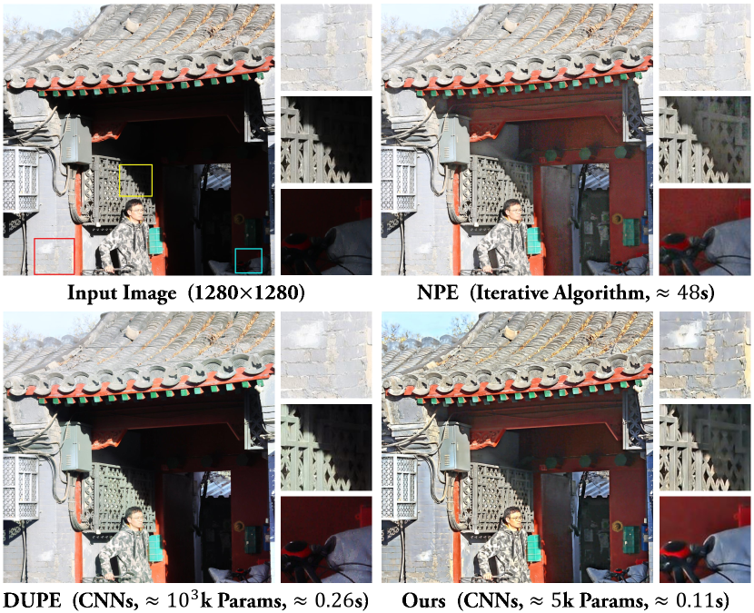
Figure 1. A challenging non-uniform illumination enhancement example. Comparing with existing methods, our solution can generate results with satisfactory visibility, vivid color, richer details and higher contrast using less time.

Non-uniform illumination image enhancement is a challenging task, as it needs to simultaneously manipulate many factors, such as color, contrast, exposure, noise, artifacts and so on. In addition, with the popularity of various camera sensors, like smartphone cameras, surveillance cameras, etc., the enhancement algorithms should be more light-weight and efficient to be applied for mobile devices and embedded systems.

Although many methods have been proposed to tackle this task in recent years, there is still large room for improvement whether in terms of performance or effect, as shown in Figure 1. Histogram equalization (HE) and Retinex theory (Land, 1977) are two typical traditional enhancement methods. HE-based algorithms (Ibrahim and Kong, 2007; Arici et al., 2009; Nakai et al., 2013; Celik and Tjahjadi, 2011; Lee et al., 2013a) focus on improving the global contrast by stretching the dynamic range of images, which will result in limited local details and unnatural color. Retinex-based methods (Jobson et al., 1997a; Lee et al., 2013b; Fu et al., 2016; Guo et al., 2017; Li et al., 2018) try to recover the contrast by using the estimated illumination map. Mostly, they focus on restoring brightness and contrast while ignoring the influences of noise and artifacts. Learning-based methods (Lore et al., 2017; Lv et al., 2018; Gharbi et al., 2017; Wei et al., 2018; Ren et al., 2019) usually utilize heavy-weight and complex network architecture to deal with brightness, contrast, color and noise, which are difficult to apply to some real-time scenes or mobile devices. Besides, Learning-based methods need large images for training and the performance is limited by the quality of training dataset.

Therefore, in this paper, we first propose a novel semi-supervised pipeline to construct a paired image dataset for non-uniform illumination enhancement. Following the above pipeline, we build a paired dataset based on Microsoft COCO dataset (Lin et al., 2014), which contains numerous real-world image pairs with various exposure conditions. This dataset can be an efficient benchmark for enhancement researches. Based on this dataset, we design a novel network for non-uniform illumination enhancement. In detail, it first enhances the non-uniform illumination images from both under- and over-expose aspects based on the Retinex model. Then, the different enhanced intermediate results are fused to generate the exposure corrected result. After that, the extra noise and compression artifacts are removed to get the final result. Our model is more light-weight ($\approx 5$k parameters) and faster (enhance 0.5 mega-pixel images in real-time) than existing enhancement methods. Comprehensive experiments demonstrate that our method is superior to state-of-the-art methods in both qualitative and quantitative.

Overall, our contributions are in three folds:

• We propose a novel light-weight network for non-uniform illumination enhancement, which can enhance images in real-time. It not only keeps the advantages of robustness of Retinex model but also overcomes the limitation of unable to enhance under-/over-exposure regions simultaneously.

• We construct a new large-scale dataset ($\approx 82$k image pairs) for non-uniform illumination enhancement benchmarking and researching.

• Comprehensive experiments have been conducted to demonstrate that our method outperforms state-of-the-art methods qualitatively and quantitatively.

2. Related Work

Image enhancement has been studied and developed for a long time. In this section, we will make a brief overview of the most related methods.

Traditional enhancement methods. Histogram equalization (HE) is a widely used technique by redistributing the luminous intensity on histogram. A lot of HE-based methods are proposed using additional priors and constraints. BPDHE (Ibrahim and Kong, 2007) preserves the mean brightness of the image to avoid unnecessary visual deterioration; Arici et al. (Arici et al., 2009) regards enhancement as an optimization problem and introduces specifically designed penalty terms; DHECI (Nakai et al., 2013) utilizes differential gray-levels histogram that contains edge information. These methods, however, focus on improving the contrast of the entire image without considering the illumination. Therefore, over- and under-enhancement often occur after adjustment.

Retinex theory (Land, 1977) supposes that an image is composed of reflection and illumination. Thus, MSR (Jobson et al., 1997a) and SSR (Jobson et al., 1997b), recover and make use of the illumination map for low-light image enhancement. Furthermore, NPE (Wang et al., 2013) makes a balance between details and naturalness. MF (Fu et al., 2016) proposes a fusion-based method for weak illumination images. LIME (Guo et al., 2017) develops a structure-aware smoothing model to improve the illumination consistency. BIMEF (Ying et al., 2017a) designs a multi-exposure fusion framework, and Ying et al. (Ying et al., 2017b) combine the camera response model and traditional Retinex model. Mading et al. (Li et al., 2018) consider a noise map for enhancing low-light images accompanied by intensive noise. However, most methods rely on hand-crafted illumination map and careful parameter tuning while can not deal well with noise and artifacts.

Learning-based enhancement methods. The past few years have witnessed the fast development of deep learning in the field of image enhancement. LLNet (Lore et al., 2017) trains a stacked sparse denoising autoencoder to learn the brightening and denoising functions. HDRNet (Gharbi et al., 2017) designs an architecture to make local, global, and content-dependent decisions to approximate the desired image transformation. RetinexNet (Wei et al., 2018) combines the Retinex theory with CNN and KinD (Zhang et al., 2019b) adds a Restoration-Net for noise removal. Wenqi et al. (Ren et al., 2019) use two distinct streams in hybrid network to simultaneously learn the global content and the salient structures. DeepUPE (Wang et al., 2019) introduces intermediate illumination in our network to associate the input with expected enhancement result, whereas it doesn’t consider the noise in the low-light image. Besides, DPED (Ignatov et al., 2017) uses a residual CNN to transform cameras from common smartphones into high-quality DSLR cameras with the paired dataset. Differently, Yusheng et al. (Chen et al., 2018b) learn image enhancement by GANs from a set of unpaired photographs with the user’s desired characteristics. As for extremely low-light scenes, SID (Chen et al., 2018a) proposes a paired dataset and develops an end-to-end pipeline to directly process raw sensor images. Most of these learning-based methods don’t explicitly contain the denoising module, and some rely on traditional denoising methods with unsatisfactory results. What’s more, these methods can not meet the real-time running demand for mobile devices.

Overall, the existing methods can hardly deal well with non-uniform illumination images both in quality and efficiency. In contrast, our approach is more light-weight and faster, and can enhance under-/over-exposure regions and restore the degradation simultaneously. Besides, our proposed dataset supplements non-uniform illumination enhancement benchmark datasets. Therefore, our method is complementary to existing methods.

3. Dataset

In this section, we first compare the proposed dataset with existing enhancement datasets to demonstrate the reason of constructing a new dataset. After that, we introduce the construction details of our new dataset.

Figure 2. Example images of our dataset. Top: non-uniform exposed images. Bottom: corresponding reference images.

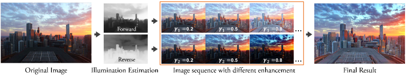
Figure 3. The pipeline of the proposed retouching module. We use the smoothness of bright channel (the maximal value of three channels) to replace the complex illumination estimation. Details can be found in Section 3.2.

3.1. Comparison with Existing Datasets

There are two prevalent solutions to obtain paired differently exposed images: multiple shooting and expert retouching. LOL (Wei et al., 2018) (altering ISO), SID (Chen et al., 2018a) (altering exposure time) and DSLR (Ignatov et al., 2017) (altering hardware) are the representative datasets of the former solution. However, multiple shooting is time-consuming and labor-intensive, which limits the size of datasets, and faces the problem of image alignment. Besides, for the high-dynamic range scenes, even DSLR is difficult to get satisfactory results by shooting only once. To this dilemma, SICE (Cai et al., 2018) collects multi-exposure image sequences and uses Exposure Fusion techniques to construct the reference images, which are difficult to avoid the situation of blur and ghosting caused by incomplete alignment. DeepUPE (Wang et al., 2019) and MIT-Adobe FiveK (Bychkovsky et al., 2011) are the representative datasets of the latter solution, and are created for enhancing under-exposed and general images respectively. However, they lack the consideration of over-exposure scenes resulting in covering limited lighting conditions. To cover various lighting conditions and scenes, we take the expert retouching solution to construct a new dataset based on Microsoft COCO dataset (Lin et al., 2014), which contains numerous real-world images with different exposure levels.

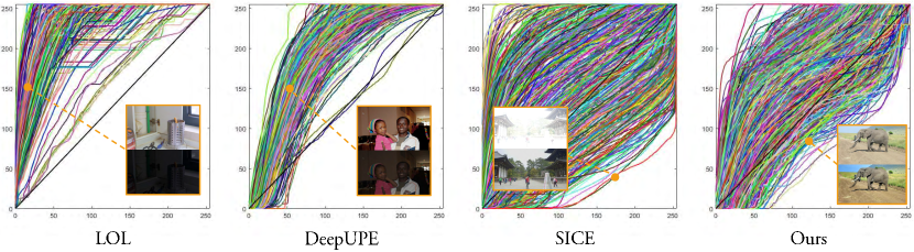
Figure 4. Existing representative enhancement datasets’ and our dataset’s statistical results of exposure adjustment curves. The small images are the example image pairs of different datasets.

To visually show the differences between different enhancement datasets, we calculate the exposure adjustment curve, which is used to adjusting the histogram of the original images’ Value component in HSV color space to match the histogram of reference images, as shown in Figure 4. On one hand, the distribution of curves can approximately indicate the exposure adjustment of the dataset. That is to say, LOL (Wei et al., 2018) and DeepUPE (Wang et al., 2019) are only used to learn to increase the exposure adaptively. SICE (Cai et al., 2018) and our dataset cover various exposure adjustments. On the other hand, the shape of the curve to some extent indicates the complexity of the adjustment. The curves of LOL (Wei et al., 2018) and SICE (Cai et al., 2018) are almost all simpler shapes similar to gamma curves, which shows that the covered light conditions are limited. As for DeepUPE (Wang et al., 2019) and our dataset, the curve shapes are more complex similar to the S-Curve. As our dataset cover under-/over-exposed simultaneously, our light conditions are more diverse result in more complex curves compared with DeepUPE (Wang et al., 2019). In summary, our dataset contains more diverse scenes and lighting conditions, which is a complement to existing datasets.

3.2. Dataset Construction Details

The Microsoft COCO dataset (Lin et al., 2014) covers diverse scenes, various resolution, different quality, manifold lighting conditions and abundant annotations, which is helpful for improving the robustness of the trained model. Therefore, we construct our new dataset based on COCO (Lin et al., 2014). We design a semi-supervised retouching solution to automatically generate our dataset, instead of adjusting the images one by one using professional tools (like Photoshop). Specifically, we first cluster images based on their histograms. Then, images of the cluster center are selected and are adjusted using our retouching module to capture optimal coefficients according to human perception. Finally, according to the clustering results, the same coefficients are used for retouching images belong to the same class. In this experiment, we use the COCO train set ($\approx 82$k images) and cluster this image empirically set to $500$ classes.

The key of our semi-supervised retouching solution is the retouching module, as shown in Figure 3. It can be formulated as:

(1) $$R_{1}\!=\!\mathcal{F}(I,\frac{I}{\mathcal{S}(max(I),\theta_{1})^{\gamma_{1}}+\epsilon},1-\frac{1-I}{\mathcal{S}(max(1-I),\theta_{2})^{\gamma_{2}}+\epsilon},\theta_{3})$$

where $I$ and $R_{1}$ represent original image and the fusion result, $\epsilon$ is a small constant preventing division by zero, $\mathcal{S}$ and $\mathcal{F}$ represents smooth (Xu et al., 2011) and fusion (Mertens et al., 2009) operation, final result $R=R_{1}+\alpha(R_{1}-\mathcal{S}(R_{1},\theta_{4}))$, {$\theta_{1},\theta_{2},\theta_{3},\theta_{4},\gamma_{1},\gamma_{2},\alpha$} are the coefficients. Notice that, {$\theta_{1},\theta_{2},\gamma_{1},\gamma_{2}$} are vectors to obtain image sequence with different enhancement. We first use the original/inverted image to enhance the under-/over-exposed regions to get preliminary enhancement sequence, and then fuse them and amplify the details to obtain the final satisfying image, inspired by (Zhang et al., 2019a; Lv and Lu, 2019). The latent principle is enhancing contrast by locally smoothing the illumination and adjusting the exposure by gamma adjustment. Since our retouching solution is robust to similar light conditions (histograms), our semi-supervised retouching solution can efficiently enhance up to 82k images quickly. Besides, we also simulate and add noise (using realistic noise model (Guo et al., 2019)) and compression artifacts (using JPEG compression) on the original COCO images, which are the two most common image degradation factors, to train our model for simultaneously suppressing noise and artifacts.

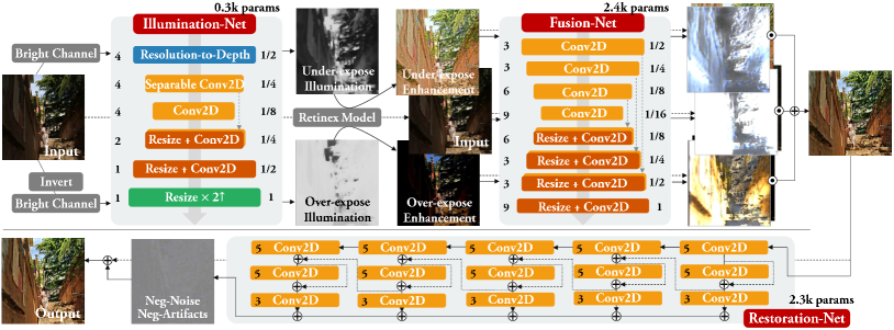
Figure 5. Overview of the proposed light-weight network architecture. The dashed lines represent skip connections. The Bright channel means the maximal value of three channels. $\odot$ and $\oplus$ represent pixel-wise multiplication and plus. The left and right numbers of every convolutional layer means the channel number and the resolution size compare with the input images.

4. Proposed Method

In this section, we introduce the proposed solution, including enhancement model, network architecture, loss function and implementation details.

4.1. Enhancement Model

The Retinex model (Land, 1977) is a robust enhancement model, which aims to learn image-to-illumination instead of image-to-image mapping. The robust version (Li et al., 2018) is formulated as: $R=I\circ L^{-1}+N$, where $I$, $L$ and $N$ represent original image, illumination map and negative noise map, $\circ$ denotes a pixel-wise multiplication. $R$ is the reflectance and usually used as the final enhancement result.

However, as the value range of the illumination map is $[0,1]$, which means the prevalent Retinex-based enhancement models do not have the ability to suppress over-exposure regions of the non-uniform illumination images. Inspired by (Zhang et al., 2019a), suppressing over-exposure regions of original images is equal to enhancing under-exposure regions of the inverted images. Thus, we can first enhance under-/over-exposure regions separately and then fusion them to generate final enhancement results (see figure 6). In this way, we can keep the advantages (illumination maps have relatively simple forms with known priors for natural images) of the Retinex model and overcome its limitations (difficulty to suppress over-exposure regions). The enhancement model can be formulated as:

(2) $$R=\mathcal{F}(I,I\circ L^{-1},1-(I_{i}\circ L_{i}^{-1}))+N,$$

where $I_{i}$ and $L_{i}$ represent inverted image and the corresponding illumination map, $\mathcal{F}()$ represents the fusion function.

4.2. Network Architecture

We propose a fully convolutional network containing three subnets: an Illumination-Net, a Fusion-Net and a Restoration-Net. Figure 5 shows the overall network architecture. As described in the enhancement model, the Illumination-Net is designed for estimating the illumination map based on the Retinex model. The Fusion-Net aims to fuse different intermediate enhanced results to generate exposure corrected images. The purpose of the Restoration-Net is to suppress the noise and compression artifacts. The detailed description is provided below.

Illumination-Net. As the illumination is at least the maximal value of three channels at a certain location, we use the maximal value of three channels as the input of the Illumination-Net. Also considering that the illumination maps have relatively simple forms with known priors for natural images, we can calculate the low-resolution illumination map and perform bilateral grid-based upsampling to enlarge the low-res prediction to approximate the full resolution illumination map (Wang et al., 2019). To avoid information loss caused by directly downsampling, we pack the input image into four channels and correspondingly reduce the spatial resolution by a factor of two in each dimension.

Fusion-Net. To better use the intermediate enhanced results, the output of the Fusion-Net is the fusion weight rather than the final fusion results. The final fusion result is formulated as:

(3) $$R_{1}=\mathcal{F}(I_{U})\circ I_{U}+\mathcal{F}(I)\circ I+\mathcal{F}(I_{O})\circ I_{O},$$

where$R_{1}$ is the fusion result, $I$, $I_{U}$ and $I_{O}$ represent original image, under-expose enhancement result and the over-expose enhancement result, $\mathcal{F}()$ represents the Fusion-Net. We directly adopt U-Net in our implementation.

Restoration-Net. According to the enhancement model, we design a light-weight multi-branch Restoration-Net to estimate the negative noise map $N$ to suppress the noise and compression artifacts, inspired by (Lv et al., 2018). Different from (Lv et al., 2018), we add skip connections between different branches to better reuse of extracted features. We directly calculate the sum of different branches’ results as the final negative noise map.

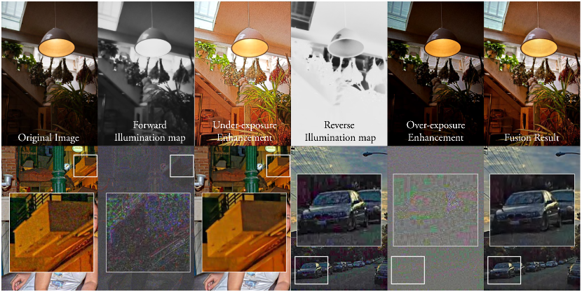
Figure 6. Examples of intermediate results of our model on real-world images. The noise map and artifacts map are normalized for better visualization.

4.3. Loss Function

We use a hierarchical strategy for training. Specifically, training is first done for Illumination-Net and Fusion-Net, which are as an end-to-end network. Then, training is done for Restoration-Net by fixing the weights of Illumination-Net and Fusion-Net. The detail loss functions of these two stages are given below.

Enhancement loss. The training for Illumination-Net and Fusion-Net aims to improve the performance of enhancement, like contrast, colorfulness, detail, etc. To improve the image quality both qualitatively and quantitatively, we design a loss function by further considering both structural and perceptual information. It can be expressed as:

(4) $$\mathcal{L}_{E}=\mathcal{L}_{h}+\mathcal{L}_{p}+\mathcal{L}_{s}+\omega_{i}\mathcal{L}_{i},$$

where the $\mathcal{L}_{h}$, $\mathcal{L}_{p}$, $\mathcal{L}_{s}$ and $\mathcal{L}_{i}$ represent Huber loss, structural loss, perceptual loss and illumination smoothness loss, and $\omega_{i}$ is the coefficient.

The Huber loss is a robust estimator and has proved to avoid the averaging problem of colorization (Zhang et al., 2017). Similarly, it is useful for increasing the color saturation of images in enhancement tasks (Atoum et al., 2019). Therefore, we use Huber loss as the basic component of the loss function:

(5) $$\mathcal{L}_{h}=\frac{1}{2}(I_{r}-\widetilde{I})^{2}\mathbbm{1}_{\{|I_{r}-\widetilde{I}|<\delta\}}+\delta(|I_{r}-\widetilde{I}|-\frac{1}{2}\delta)\mathbbm{1}_{\{|I_{r}-\widetilde{I}|\geq\delta\}},$$

where $I_{r}$ and $\widetilde{I}$ are the predicted and expected images. $\delta$ is the parameter of the Huber loss and is set to $0.5$ empirically.

To reduce the perceptual error and improve the visual quality, we introduce perceptual loss by using VGG network (Simonyan and Zisserman, 2014) as the content extractor (Ledig et al., 2017). We use the output of the ReLU activation layers of the pre-trained VGG-19 network to define the perceptual loss as:

(6) $$\mathcal{L}_{p}=\frac{1}{w_{ij}h_{ij}c_{ij}}\sum_{x=1}^{w_{ij}}\sum_{y=1}^{h_{ij}}\sum_{z=1}^{c_{ij}}\lVert\phi_{ij}(I_{r})_{xyz}-\phi_{ij}(\widetilde{I})_{xyz}\lVert,$$

where $w_{ij}$ , $h_{ij}$ and $c_{ij}$ describe the dimensions of the respective feature maps within the VGG-19 network. Besides, $\phi_{ij}$ indicates the feature map obtained by $j$-th convolution layer in $i$-th block of the VGG-19 Network.

The structural loss is introduced to preserve the image structure and avoid blurring and artifacts. We use the well-known image quality assessment algorithm SSIM (Wang et al., 2004) to estimate the structure error. It is defined as:

(7) $$\mathcal{L}_{s}=1-\frac{1}{N}\sum_{p\in img}\frac{2\mu_{x}\mu_{y}+C_{1}}{\mu_{x}^{2}+\mu_{y}^{2}+C_{1}}\cdot\frac{2\sigma_{xy}+C_{2}}{\sigma_{x}^{2}+\sigma_{y}^{2}+C_{2}},$$

where $\mu_{x}$ and $\mu_{y}$ are pixel value averages, $\sigma_{x}^{2}$ and $\sigma_{y}^{2}$ are variances, $\sigma_{xy}$ is the covariance, and $C_{1}$ and $C_{2}$ are constants to prevent the denominator to zero.

Local consistency and structure-awareness are the key hypotheses for illumination estimation in previous works (Guo et al., 2017; Wei et al., 2018; Wang et al., 2019). Following this idea, we introduce the illumination smoothness loss to smooth the textural details and preserve the overall structure boundary. We use the structure-aware TV loss define the illumination smoothness loss as:

(8) $$\mathcal{L}_{i}=\|\nabla I_{i}\circ exp(-\lambda_{g}\cdot\nabla I)\|+\|\nabla\bar{I_{i}}\circ exp(-\lambda_{g}\cdot\nabla(1-I))\|,$$

where $I_{i}$ and $\bar{I_{i}}$ are the estimated forward and reverse illumination maps, $I$ is the original image, $\nabla$ represents the gradient, $\lambda_{g}$ is the coefficient balancing the strength of structure-awareness. We set $\lambda_{g}=10$ and $\omega_{i}=0.002$ empirically.

Restoration loss. Image restoration also aims to preserve the structure, suppress noise and artifacts, and obtain satisfactory visual effects, which is the same as enhancement in some ways. Therefore, similar to the Enhancement loss, the Restoration loss is defined as:

(9) $$\mathcal{L}_{E}=\mathcal{L}_{h}+\mathcal{L}_{p}+\mathcal{L}_{s}+\omega_{g}\mathcal{L}_{g},$$

where the $\mathcal{L}_{h}$, $\mathcal{L}_{p}$ and $\mathcal{L}_{s}$ are the same as the corresponding components of the Enhancement loss. $\mathcal{L}_{g}$ represents the global TV loss and is defined as $\|\nabla{I_{r}}\|$. We empirically set $\omega_{g}=10^{-4}$ which denotes the coefficient of global TV loss.

4.4. Implementation Details

Our implementation is done with Keras (Chollet et al., 2015) and Tensorflow (Abadi et al., 2016). The proposed light-weight network can be quickly converged after being trained for $10$ epochs on an Nvidia Titan Xp GPU using the proposed dataset. We use random clipping, flipping and rotating for data augmentation to prevent over-fitting. We set the batch-size to $32$ and the size of random clipping patches to $256\times 256\times 3$. We use the output of the fourth convolutional layer in the third block of the VGG-19 network (Simonyan and Zisserman, 2014) as the perceptual loss extraction layer. The input image values of Illumination-Net and Fusion-Net are scaled to $[0,1]$, while the values are scaled to $[-1,1]$ for Restoration-Net. In the experiment, the entire network is optimized using the Adam optimizer (Kingma and Ba, 2014) with parameters of $\alpha=0.001$, $\beta_{1}=0.9$, $\beta_{2}=0.999$ and $\epsilon=10^{-8}$. We also use the learning rate decay strategy, which reduces the learning rate to $98\%$ before the next epoch. At the same time, we reduce the learning rate to $50\%$ when the loss metric has stopped improving.

5. Experimental Results

In this section, we evaluate our method through extensive experiments. We first compare our method with state-of-the-art enhancement methods in both qualitative and quantitative. Then, we present more analysis to demonstrate our method comprehensively.

5.1. Comparison with State-of-the-art Methods

We comprehensively compare our method with state-of-the-art methods by using the publicly-available codes with recommended parameter settings to show that our method is complementary to existing methods.

Visual Comparison. We provide a visual comparison to show the differences between our method and existing state-of-the-art algorithms. Typical challenging cases are shown in Figure 7.

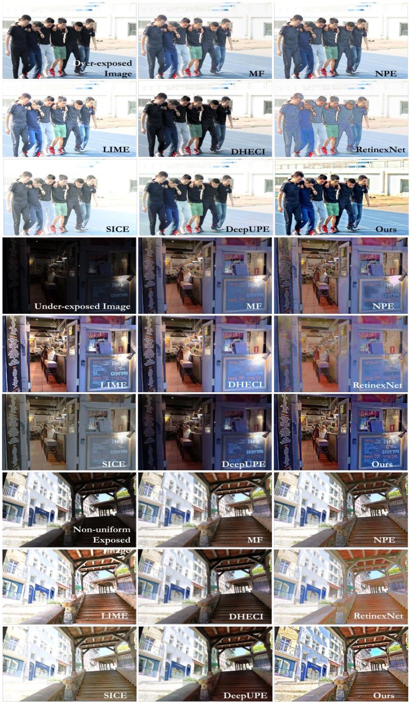
Figure 7. Visual comparison of real-world challenging non-uniform exposed images. Please zoom in for a better view.

For the first over-exposed scene, enhancing dark clothes is challenging as they are easily confused with under-exposed regions. This dilemma is especially serious for Retinex-based methods, like RetinexNet (Wei et al., 2018) and LIME (Guo et al., 2017). Our method can avoid this problem to some extent by image fusion strategy. Besides, for over-exposed regions like runways and stands, these methods fail to enhance them. In contrast, our method effectively enhances over-exposed regions and obtain high contrast and rich color.

For the second under-exposed scene, insufficient enhancement (like DeepUPE (Wang et al., 2019)), color degradation (like SICE (Cai et al., 2018)), and local over-enhancement (see regions of the light source in NPE (Wang et al., 2013)) are flaws of existing methods. In contrast, our method is able to reveal vivid colors, avoid over-/under- enhancement, and improve the details simultaneously.

For the last scene, over-/under-exposed regions need to be enhanced simultaneously. Existing methods tend to enhance under-exposed regions but ignore the over-exposed ones. Our method effectively enhances different exposed regions simultaneously and amplifies the contrast, which makes results more appealing.

In addition, our method is able to enhance the 720p video frame-by-frame almost in real-time. Our method also outperforms these methods on video enhancement. Please check the supplementary materials for details.

Quantitative Comparison. To evaluate the inference performance and generalization capability of our solution, we quantitatively compare it with the other methods. For a fair comparison of generalization capability, we build a test set contains 50 various exposed images selected from existing paired public enhancement datasets (15 images from LOL (Wei et al., 2018), 15 images from SICE (Cai et al., 2018) and 20 images from DeepUPE (Wang et al., 2019)). Tables 1 reports the comparison results, where for every method, we use the pre-trained weights or recommended parameters. Our result performances well in all quality metrics, which fully demonstrates the outperformance of our approach.

Table 1. Quantitative comparison results. The average runtime is tested using images with size $1280\times 720$. “*” represents only using an Intel i5-8400 CPU.

Algorithm	$\uparrow$PSNR	$\uparrow$SSIM (Wang et al., 2004)	$\uparrow$VIF (Sheikh and Bovik, 2006)	$\downarrow$LOE (Ying et al., 2017a)	$\downarrow$NIQE(Mittal et al., 2012)	Params	Runtime
*MSR (Jobson et al., 1997a)	11.87	0.56	0.41	2029.4	4.19	-	1.44s
Dong (Dong et al., 2011)	13.82	0.54	0.33	1598.0	4.91	-	0.43s
BPDHE (Ibrahim and Kong, 2007)	14.41	0.57	0.34	892.2	4.21	-	0.49s
NPE (Wang et al., 2013)	14.95	0.58	0.38	1563.7	4.31	-	25.6s
DHECI (Nakai et al., 2013)	16.14	0.58	0.39	903.3	4.62	-	42.3s
MF (Fu et al., 2016)	16.10	0.62	0.39	1113.1	4.51	-	0.83s
LIME (Guo et al., 2017)	12.49	0.53	0.42	1441.2	4.68	-	0.56s
BIMEF (Ying et al., 2017a)	15.58	0.66	0.40	857.1	3.97	-	0.54s
SICE (Cai et al., 2018)	14.63	0.62	0.31	1312.2	4.24	682k	1.81s
RetinexNet (Wei et al., 2018)	12.84	0.51	0.31	2278.2	5.07	445k	0.16s
GLADNet (Wang et al., 2018)	17.71	0.68	0.36	949.9	3.87	932k	0.38s
MBLLEN (Lv et al., 2018)	18.06	0.71	0.33	898.1	3.06	450k	0.31s
DeepUPE (Wang et al., 2019)	16.48	0.65	0.40	871.4	3.69	100k	0.10s
Ours	17.83	0.73	0.42	869.7	3.03	5k	0.05s

For inference performance, our method significantly outperforms other methods. Our model is very lightweight, which makes it potentially useful for mobile devices. Besides, the inference speed of our model is very fast. It can enhance 0.5 mega-pixel images in real-time and 720p video in almost real-time (20f/s).

User Study. To test the subjective preference of non-uniform exposed image enhancement methods, we conduct a user study with $50$ participants. We randomly select $20$ natural non-uniform exposed images and enhance them using our method and other five representative methods. For each case, the original image and six enhanced results are displayed to the participants simultaneously in a random arrangement. Then, the participants are asked to rank the quality of the six enhancements from 1 (best) to 6 (worst) for each of the four questions. We also provide zoom-in function to let participants check details. Figure 8 shows the statistical result of the user study, where every sub-figure summarizes the rating distribution of a particular question. Our method receives more “best” ratings, which shows that our method is more preferred by human subjects.

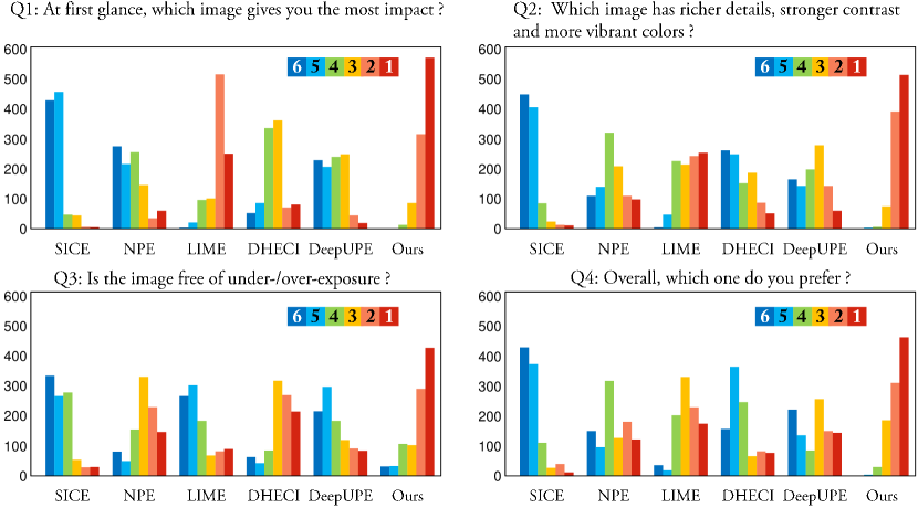
Figure 8. Rating distributions on four questions of our user study. The ordinate axis is the ranking frequency received by the methods from the participants.

Face Detection at night. Image enhancement aims to improve visibility and reflect clear details of target scenes, which are critical to many vision-based techniques especially under poor conditions. We take face detection at night as an example to investigate the effects of different enhancement methods for improving detection performance. We use the DARK FACE dataset (Yuan et al., 2019) for testing, which contains 10k low-light images with corresponding face annotation. We use the pre-trained light-weight version of DSFD (Li et al., 2019), which is the state-of-the-art deep face detector, to investigate the performance of real-time detection. To clearly demonstrate the gap between different enhancement algorithms, we select 500 “easy” images for evaluation by using the DARK FACE evaluation tool. The comparison of precision-recall (P-R) curves and the average precisions (AP) are shown in Figure 9. All these enhancement methods are beneficial to improve detection performance. Among these methods, our method and MF (Fu et al., 2016) perform best, which means to some extent that our results can effectively and realistically reflect the details of real scenes. Besides, compared with MF (Fu et al., 2016), our method is faster and can be trained together with face detectors which means that our method is more appealing in real applications.

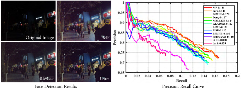
Figure 9. Face detection result comparison. Left: An intuitive example of visual comparison. Right: precision-recall curves and average precisions of after enhanced using different methods. “dark” means the result of original images without any pre-processing.

5.2. More Analysis

We provide more analysis to explore the role of components of our model and discuss the flexibility, extendibility and limitation of our method.

Why our Model Works? As illumination maps of natural images typically have relatively simple forms with known priors, learning an image-to-illumination mapping is easier than image-to-image mapping on photographic adjustment under diverse lighting conditions (Wang et al., 2019). Hence, our Illumination-Net has ability to customizing the inputs (like adjusting exposure and contrast) to the Fusion-Net by formulating constraints (like adjusting illumination magnitudes and enforcing locally smooth) on the estimated illumination map, as shown in Figre 10. However, according to the Retinex model, using a single illumination map fails to enhance both under-/over-exposed areas simultaneously.

Therefore, to overcome this dilemma, we introduce two illumination maps for enhancing under-exposure and suppressing over-exposure respectively and fuse them using Fusion-Net by estimating the fusion weight map. The final results can be customized by adjusting the fusion weight map, which provides stronger generalization capabilities and learning capabilities for our model to learn complex adjustment for both under-exposure and over-exposure regions simultaneously.

To demonstrate the good generalization capability of our network, we directly fuse real multi-exposure images using our Fusion-Net without any fine-tuning. Our fusion result is comparable with the latest fusion methods as shown in Figure 10, which shows the good adaptability and robustness of our network. In summary, our model has strong generalization and learning capabilities to learn and enhance non-uniform exposed images adaptively.

\begin{overpic}[width=433.62pt]{images/why.pdf} \put(111.0,53.0){\bf\color[rgb]{0,0,0}\tiny\cite[citep]{(\@@bibref{AuthorsPhrase1Year}{kou2017multi}{\@@citephrase{, }}{})}} \put(170.0,53.0){\bf\color[rgb]{0,0,0}\tiny\cite[citep]{(\@@bibref{AuthorsPhrase1Year}{mertens2009exposure}{\@@citephrase{, }}{})}} \end{overpic}

Figure 10. Top: Multi-Exposure Fusion comparison with MEF methods. Bottom: Illumination maps estimation comparison with typical Retinex-based methods.

Interactive Enhancement. Considering that the assessment of enhancement results is subjective, providing interactive enhancement is necessary for some application scenes. We formulate the interactive enhancement model as:

(10) $$R\!=\!\mathcal{F}(I,I/({L}^{\gamma_{1}}+\epsilon),1-I_{i}/({L_{i}}^{\gamma_{2}}+\epsilon))+\mathcal{D}^{-1}(\Phi(\mathcal{D}(N),\gamma_{3})),$$

where $I$, $L$, $N$ and $R$ represent original image, illumination map, estimated negative noise and the final interactive results, $I_{i}$ and $L_{i}$ represent inverted image and the correspond illumination map, $\epsilon$ is a small constant preventing division by zero. $\mathcal{F}$ represents fusion operation, $\mathcal{D}$ and $\mathcal{D}^{-1}$ are discrete cosine transform (DCT) and the inverse transform, $\Phi()$ represents retaining high-frequency components and setting others to zero. $\gamma_{1}$,$\gamma_{2}$ and $\gamma_{3}$ are the interactive coefficients, which control enhancing under-exposed regions, suppressing over-exposed areas and noise removal, respectively. We set the value range of $\gamma_{1}$,$\gamma_{2}$ and $\gamma_{3}$ to $[0,1]$. The larger value of $\gamma_{1}$ ($\gamma_{2}$), the stronger enhancement of under-exposed (over-exposed) regions, as shown in Figure 11. Similarly, larger value of $\gamma_{3}$ means more noise are removed. Proper $\gamma_{3}$ makes a trade-off between denoising and texture retaining.

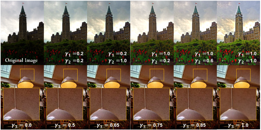
Figure 11. Examples of interactive enhancement and interactive noise removal.

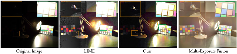
Figure 12. A Failure case. The missing details can be found in the MEF results (using 18 images for fusion).

Ablation Study. We quantitatively evaluate the effectiveness of different components in our method based on our proposed dataset using PSNR and SSIM (Wang et al., 2004) as the metrics, as shown in Table 2. Note that the Restoration-Net is not considered in this study. Directly learning image-to-image mapping using light-weight network will severely reduce enhancement quality (condition 1-2), which shows the effectiveness of our network architecture. We use $mse$ as the naive loss function under condition 2. The results (condition 3-6) show that the quality of enhancement is improving by containing more loss components. For the effect of model size, larger models bring little gain (especially for visual perception), but lighter networks reduce the quality severely (condition 7-8).

Table 2. Ablation study. This table reports the performance under each condition based on our proposed dataset. In this table, ”w/o” means without.

Condition	PSNR	SSIM
1. U-Net ($\approx 3.0$k params)	18.63	0.78
2. cGAN ($\approx 3.0$k params)	17.46	0.71
3. w/o $\mathcal{L}_{h}$, w/o $\mathcal{L}_{s}$, w/o $\mathcal{L}_{p}$, w/o $\mathcal{L}_{i}$	20.26	0.87
4. with $\mathcal{L}_{h}$, w/o $\mathcal{L}_{s}$, w/o $\mathcal{L}_{p}$, w/o $\mathcal{L}_{i}$	21.01	0.86
5. with $\mathcal{L}_{h}$, with $\mathcal{L}_{s}$, w/o $\mathcal{L}_{p}$, w/o $\mathcal{L}_{i}$	20.92	0.90
6. with $\mathcal{L}_{h}$, with $\mathcal{L}_{s}$, with $\mathcal{L}_{p}$, w/o $\mathcal{L}_{i}$	21.85	0.90
7. Dwindling model ($\approx 1.5$k params)	20.06	0.87
8. Enlarging model ($\approx 9.1$k params)	22.89	0.91
9. Proposed ($\approx 2.7$k params)	22.68	0.92

Limitation. Our method can produce satisfactory results for most non-uniform exposed images as validated above. However, for those regions without any trace of texture (complete under-exposure or over-exposure), our method fails to recover the details. Figure 12 presents an example case where our method, as well as other state-of-the-art methods, all fail to produce satisfying results.

6. Conclusions

We propose an end-to-end light-weight network for non-uniform illumination image enhancement. Different from Retinex-based methods, our method can suppress over-exposure regions by enhancing under-exposure regions of the inverted version, which keeps the advantages (illumination maps have relatively simple forms with known priors) of the Retinex model and overcome its limitations (unable to enhance over-/under-exposure regions simultaneously). We also propose a semi-supervised retouching solution to construct a new dataset ($\approx 82$k image pairs) for our network to handle color, exposure, contrast, noise and artifacts, etc., simultaneously and effectively. Extensive experiments demonstrate the effectiveness of our model. Our network only has $5000$ parameters and can enhance 0.5 mega-pixel images in real-time ($\approx 50$ fps), which is faster than existing enhancement algorithms.

Our future work will focus on recovering the missing image content for extremely under-exposed or over-exposed regions (see Figure 12) by using semantics information guided or texture synthesis techniques.

References

- (1)
- Abadi et al. (2016) Martín Abadi, Ashish Agarwal, Paul Barham, et al. 2016. Tensorflow: Large-scale machine learning on heterogeneous distributed systems. arXiv preprint arXiv:1603.04467 (2016).
- Arici et al. (2009) Tarik Arici, Salih Dikbas, and Yucel Altunbasak. 2009. A histogram modification framework and its application for image contrast enhancement. IEEE Transactions on image processing (TIP) 18, 9 (2009), 1921–1935.
- Atoum et al. (2019) Yousef Atoum, Mao Ye, Liu Ren, Ying Tai, and Xiaoming Liu. 2019. Color-wise Attention Network for Low-light Image Enhancement. arXiv preprint arXiv:1911.08681 (2019).
- Bychkovsky et al. (2011) Vladimir Bychkovsky, Sylvain Paris, Eric Chan, and Frédo Durand. 2011. Learning photographic global tonal adjustment with a database of input/output image pairs. In CVPR 2011. IEEE, 97–104.
- Cai et al. (2018) Jianrui Cai, Shuhang Gu, and Lei Zhang. 2018. Learning a Deep Single Image Contrast Enhancer from Multi-Exposure Images. IEEE Transactions on Image Processing (TIP) 27, 4 (2018), 2049–2062.
- Celik and Tjahjadi (2011) Turgay Celik and Tardi Tjahjadi. 2011. Contextual and variational contrast enhancement. IEEE Transactions on Image Processing (TIP) 20, 12 (2011), 3431–3441.
- Chen et al. (2018a) Chen Chen, Qifeng Chen Chen, Jia Xu, and Vladlen Koltun. 2018a. Learning to See in the Dark. In IEEE Conference on Computer Vision and Pattern Recognition (CVPR).
- Chen et al. (2018b) Yu-Sheng Chen, Yu-Ching Wang, Man-Hsin Kao, and Yung-Yu Chuang. 2018b. Deep photo enhancer: Unpaired learning for image enhancement from photographs with gans. In IEEE Conference on Computer Vision and Pattern Recognition (CVPR). 6306–6314.
- Chollet et al. (2015) François Chollet et al. 2015. Keras. https://github.com/keras-team/keras.
- Dong et al. (2011) Xuan Dong, Guan Wang, Yi Pang, Weixin Li, Jiangtao Wen, Wei Meng, and Yao Lu. 2011. Fast efficient algorithm for enhancement of low lighting video. In IEEE International Conference on Multimedia and Expo (ICME). IEEE, 1–6.
- Fu et al. (2016) Xueyang Fu, Delu Zeng, Yue Huang, Yinghao Liao, Xinghao Ding, and John Paisley. 2016. A fusion-based enhancing method for weakly illuminated images. Signal Processing 129 (2016), 82–96.
- Gharbi et al. (2017) Michaël Gharbi, Jiawen Chen, Jonathan T Barron, Samuel W Hasinoff, and Frédo Durand. 2017. Deep bilateral learning for real-time image enhancement. ACM Transactions on Graphics (TOG) 36, 4 (2017), 118.
- Guo et al. (2019) Shi Guo, Zifei Yan, Kai Zhang, Wangmeng Zuo, and Lei Zhang. 2019. Toward convolutional blind denoising of real photographs. IEEE Conference on Computer Vision and Pattern Recognition (CVPR) (2019).
- Guo et al. (2017) Xiaojie Guo, Yu Li, and Haibin Ling. 2017. LIME: Low-light image enhancement via illumination map estimation. IEEE Transactions on Image Processing (TIP) 26, 2 (2017), 982–993.
- Ibrahim and Kong (2007) Haidi Ibrahim and Nicholas Sia Pik Kong. 2007. Brightness preserving dynamic histogram equalization for image contrast enhancement. IEEE Transactions on Consumer Electronics 53, 4 (2007), 1752–1758.
- Ignatov et al. (2017) Andrey Ignatov, Nikolay Kobyshev, Radu Timofte, Kenneth Vanhoey, and Luc Van Gool. 2017. DSLR-quality photos on mobile devices with deep convolutional networks. In IEEE International Conference on Computer Vision (ICCV). 3277–3285.
- Jobson et al. (1997a) Daniel J Jobson, Zia-ur Rahman, and Glenn A Woodell. 1997a. A multiscale retinex for bridging the gap between color images and the human observation of scenes. IEEE Transactions on Image processing (TIP) 6, 7 (1997), 965–976.
- Jobson et al. (1997b) Daniel J Jobson, Zia-ur Rahman, and Glenn A Woodell. 1997b. Properties and performance of a center/surround retinex. IEEE Transactions on Image processing (TIP) 6, 3 (1997), 451–462.
- Kingma and Ba (2014) Diederik P Kingma and Jimmy Ba. 2014. Adam: A method for stochastic optimization. arXiv preprint arXiv:1412.6980 (2014).
- Kou et al. (2017) Fei Kou, Zhengguo Li, Changyun Wen, and Weihai Chen. 2017. Multi-scale exposure fusion via gradient domain guided image filtering. In 2017 IEEE International Conference on Multimedia and Expo (ICME). IEEE, 1105–1110.
- Land (1977) Edwin H Land. 1977. The retinex theory of color vision. Scientific American 237, 6 (1977), 108–129.
- Ledig et al. (2017) Christian Ledig, Lucas Theis, Ferenc Huszár, et al. 2017. Photo-realistic single image super-resolution using a generative adversarial network. IEEE conference on computer vision and pattern recognition (CVPR) (2017), 4681–4690.
- Lee et al. (2013a) Chulwoo Lee, Chul Lee, and Chang-Su Kim. 2013a. Contrast enhancement based on layered difference representation of 2D histograms. IEEE transactions on image processing (TIP) 22, 12 (2013), 5372–5384.
- Lee et al. (2013b) Chang-Hsing Lee, Jau-Ling Shih, Cheng-Chang Lien, and Chin-Chuan Han. 2013b. Adaptive multiscale retinex for image contrast enhancement. In Signal-Image Technology & Internet-Based Systems (SITIS). IEEE, 43–50.
- Li et al. (2019) Jian Li, Yabiao Wang, Changan Wang, et al. 2019. DSFD: dual shot face detector. In Proceedings of the IEEE Conference on Computer Vision and Pattern Recognition. 5060–5069.
- Li et al. (2018) Mading Li, Jiaying Liu, Wenhan Yang, Xiaoyan Sun, and Zongming Guo. 2018. Structure-revealing low-light image enhancement via robust Retinex model. IEEE Transactions on Image Processing (TIP) 27, 6 (2018), 2828–2841.
- Lin et al. (2014) Tsung-Yi Lin, Michael Maire, Serge Belongie, et al. 2014. Microsoft coco: Common objects in context. In European conference on computer vision (ECCV). Springer, 740–755.
- Lore et al. (2017) Kin Gwn Lore, Adedotun Akintayo, and Soumik Sarkar. 2017. LLNet: A deep autoencoder approach to natural low-light image enhancement. Pattern Recognition (PR) 61 (2017), 650–662.
- Lv and Lu (2019) Feifan Lv and Feng Lu. 2019. Attention-guided Low-light Image Enhancement. arXiv preprint arXiv:1908.00682 (2019).
- Lv et al. (2018) Feifan Lv, Feng Lu, Jianhua Wu, and Chongsoon Lim. 2018. MBLLEN: Low-light Image/Video Enhancement Using CNNs. British Machine Vision Conference (BMVC) (2018).
- Mertens et al. (2009) Tom Mertens, Jan Kautz, and Frank Van Reeth. 2009. Exposure fusion: A simple and practical alternative to high dynamic range photography. In Computer graphics forum, Vol. 28. Wiley Online Library, 161–171.
- Mittal et al. (2012) Anish Mittal, Rajiv Soundararajan, and Alan C Bovik. 2012. Making a “completely blind” image quality analyzer. IEEE Signal Processing Letters 20, 3 (2012), 209–212.
- Nakai et al. (2013) Keita Nakai, Yoshikatsu Hoshi, and Akira Taguchi. 2013. Color image contrast enhacement method based on differential intensity/saturation gray-levels histograms. In Intelligent Signal Processing and Communications Systems (ISPACS). IEEE, 445–449.
- Ren et al. (2019) Wenqi Ren, Sifei Liu, Lin Ma, Qianqian Xu, Xiangyu Xu, Xiaochun Cao, Junping Du, and Ming-Hsuan Yang. 2019. Low-Light Image Enhancement via a Deep Hybrid Network. IEEE Transactions on Image Processing (TIP) (2019).
- Sheikh and Bovik (2006) Hamid R Sheikh and Alan C Bovik. 2006. Image information and visual quality. IEEE Transactions on image processing (TIP) 15, 2 (2006), 430–444.
- Simonyan and Zisserman (2014) Karen Simonyan and Andrew Zisserman. 2014. Very Deep Convolutional Networks for Large-Scale Image Recognition. Computer Science (2014).
- Wang et al. (2019) Ruixing Wang, Qing Zhang, Chi-Wing Fu, Xiaoyong Shen, Wei-Shi Zheng, and Jiaya Jia. 2019. Underexposed Photo Enhancement Using Deep Illumination Estimation. In IEEE Conference on Computer Vision and Pattern Recognition (CVPR). 6849–6857.
- Wang et al. (2013) Shuhang Wang, Jin Zheng, Hai-Miao Hu, and Bo Li. 2013. Naturalness preserved enhancement algorithm for non-uniform illumination images. IEEE Transactions on Image Processing (TIP) 22, 9 (2013), 3538–3548.
- Wang et al. (2018) Wenjing Wang, Chen Wei, Wenhan Yang, and Jiaying Liu. 2018. GLADNet: Low-Light Enhancement Network with Global Awareness. In IEEE International Conference on Automatic Face & Gesture Recognition (FG). IEEE, 751–755.
- Wang et al. (2004) Zhou Wang, Alan C Bovik, Hamid R Sheikh, and Eero P Simoncelli. 2004. Image quality assessment: from error visibility to structural similarity. IEEE transactions on image processing (TIP) 13, 4 (2004), 600–612.
- Wei et al. (2018) Chen Wei, Wenjing Wang, Wenhan Yang, and Jiaying Liu. 2018. Deep Retinex Decomposition for Low-Light Enhancement. British Machine Vision Conference (BMVC) (2018).
- Xu et al. (2011) Li Xu, Cewu Lu, Yi Xu, and Jiaya Jia. 2011. Image smoothing via L 0 gradient minimization. In ACM Transactions on Graphics (TOG), Vol. 30. ACM, 174.
- Ying et al. (2017a) Zhenqiang Ying, Ge Li, and Wen Gao. 2017a. A Bio-Inspired Multi-Exposure Fusion Framework for Low-light Image Enhancement. arXiv preprint arXiv:1711.00591 (2017).
- Ying et al. (2017b) Zhenqiang Ying, Ge Li, Yurui Ren, Ronggang Wang, and Wenmin Wang. 2017b. A new low-light image enhancement algorithm using camera response model. In IEEE International Conference on Computer Vision (ICCV). 3015–3022.
- Yuan et al. (2019) Ye Yuan, Wenhan Yang, Wenqi Ren, Jiaying Liu, Walter J Scheirer, and Zhangyang Wang. 2019. UG Track 2: A Collective Benchmark Effort for Evaluating and Advancing Image Understanding in Poor Visibility Environments. arXiv preprint arXiv:1904.04474 (2019).
- Zhang et al. (2019a) Qing Zhang, Yongwei Nie, and Wei-Shi Zheng. 2019a. Dual Illumination Estimation for Robust Exposure Correction. In Computer Graphics Forum, Vol. 38. Wiley Online Library, 243–252.
- Zhang et al. (2017) Richard Zhang, Jun-Yan Zhu, Phillip Isola, Xinyang Geng, Angela S Lin, Tianhe Yu, and Alexei A Efros. 2017. Real-Time User-Guided Image Colorization with Learned Deep Priors. ACM Transactions on Graphics (TOG) 9, 4 (2017).
- Zhang et al. (2019b) Yonghua Zhang, Jiawan Zhang, and Xiaojie Guo. 2019b. Kindling the Darkness: A Practical Low-light Image Enhancer. arXiv preprint arXiv:1905.04161 (2019).