Generation and distribution of atomic entanglement in coupled-cavity arrays

Abstract

We study the dynamics of entanglement in a 1D coupled-cavity array, each cavity containing a two-level atom, via the Jaynes-Cummings-Hubbard (JCH) Hamiltonian in the single-excitation sector. The model features a rich variety of dynamical regimes that can be harnessed for entanglement control. The protocol is based on setting an excited atom above the ground state and further letting it evolve following the natural dynamics of the Hamiltonian. Here we focus on the concurrence between pairs of atoms and its relation to atom-field correlations and the structure of the array. We show that the extension and distribution pattern of pairwise entanglement can be manipulated through a judicious tuning of the atom-cavity coupling strength only. Our work offers a comprehensive account over the machinery of the single-excitation JCH Hamiltonian as well as contributes to the design of hybrid light-matter quantum networks.

I Introduction

Quantum entanglement is one of the most intriguing properties of nature with no classical analog Horodecki et al. (2009). It is a key manifestation in many-body physics for it plays a significant role in quantum phase transitions Amico et al. (2008); Vidal et al. (2003); Osterloh et al. (2002). In addition, entanglement is a fundamental resource in quantum information processing tasks such as teleportation Bennett et al. (1993), quantum cryptography Ekert (1991); Gisin et al. (2002) and quantum dense coding Bennett and Wiesner (1992), to name a few. In this respect, in order to properly design such a class of protocols one must be able to faithfully transmit quantum states and establish entanglement over arbitrarily distant parties (qubits) DiVincenzo (1995); Cirac et al. (1997). Setting reliable quantum communication channels is thus a primary step towards building large-scale quantum networks Kimble (2008); Schoelkopf and Girvin (2008).

Along those lines, photonic channels stand out as current technology allows for light propagation over large distances with negligible decoherence. On top of that, local quantum information processing units (nodes) may consist of single atoms placed in optical resonators. This allows for light-matter interfacing with high degree of control, thanks to experimental advances in cavity-QED-based architectures Ritter et al. (2012); Nölleke et al. (2013); Reiserer et al. (2014); Reiserer and Rempe (2015).

A paradigmatic framework to deal with coupled-cavity systems is the Jaynes-Cummings-Hubbard (JCH) model, where cavities containing single two-level atoms are brought together enough to allow for photon tunneling. Atom-cavity coupling is given by the acclaimed Jaynes-Cummings interaction in the rotating-wave approximation. Early developments of the model initiated with the discovery that it displays a superfluid to Mott insulator quantum phase transition Greentree et al. (2006); Angelakis et al. (2007). This established coupled-cavity systems also as potential many-body quantum simulators Tomadin and Fazio (2010). Furthermore, the hybrid light-matter nature of the excitations unveils novel phases of matter Rossini and Fazio (2007) and can also be useful for quantum information processing tasks Almeida et al. (2016) (for reviews on the model and related content, see Refs. Hartmann et al. (2008); Tomadin and Fazio (2010)).

In this work, we further explore the versatility of a 1D coupled-cavity array in order to generate and distribute entanglement, which is a key element in the design of quantum networks Kimble (2008). The protocol is based on preparing a impurity – here, an excited atom – over a well-defined ground state and let it evolve following the natural, Hamiltonian dynamics of the system. Along the process it is possible to generate entanglement as shown for spin chains in Refs. Amico et al. (2004); Almeida et al. (2017) (cf. Fukuhara et al. (2015) for an experimental realization). Here the initial atomic excitation is released from the middle of a coupled-cavity array prepared in the vacuum state (no photons) with all the remaining atoms in their ground state. As the JCH model commutes with the total number operator, the dynamics ends up being restricted to the single-excitation subspace what allows for easy analytical treatment Makin et al. (2009) in addition to displaying very rich properties Makin et al. (2009); Ciccarello (2011); Almeida et al. (2016, 2017).

We carry out a detailed analysis over limiting interaction regimes of the JCH Hamiltonian and track entanglement evolution over time in two forms: the von Neumann entropy for the whole atomic component in regard to the photonic degrees of freedom and the concurrence between atomic pairs. We discuss the role of atom-field entropy in establishing atomic entanglement and how its spatial distribution profile is related to the atom-cavity interaction strength and the structure of the embedded array.

In the following Sec. II, we introduce the JCH Hamiltonian. In Sec. III, the weak- and strong-coupling regimes of the model is addressed in detail. In Sec. IV we outline the entanglement signatures of interest and discuss their dynamics focusing on those limiting regimes. Conclusions are drawn in Sec. V.

II Jaynes-Cumming-Hubbard model

We consider an one-dimensional array of $N$ high-quality coupled cavities, each containing a single two-level atom, with $\ket{g}$ and $\ket{e}$ denoting the ground and excited states, respectively. Each atom interacts with the field through the local Jaynes-Cummings (JC) Hamiltonian (in the rotating-wave approximation) Jaynes and Cummings (1963)

$$H_{x}^{\mathrm{JC}}=\omega_{c}a_{x}^{\dagger}a_{x}+\omega_{a}\sigma_{x}^{+}\sigma_{x}^{-}+g(\sigma_{x}^{+}a_{x}+\sigma_{x}^{-}a_{x}^{\dagger}),$$ (1)

where $a_{x}^{\dagger}$ ($a_{x}$) and $\sigma_{x}^{+}$ ($\sigma_{x}^{-}$) are, respectively, the bosonic and atomic raising (lowering) operators acting on the $x$-th cavity, $g$ is the atom-field coupling strength, $\omega_{c}$ is the cavity frequency, and $\omega_{a}$ is the atomic transition frequency. We set $\hbar=1$ for convenience. The eigenstates of Hamiltonian (1) are dressed (hybrid) states featuring photonic and atomic excitations known as polaritons, which in resonance ($\Delta=\omega_{a}-\omega_{c}=0$) read $\ket{n\pm}_{x}=(\ket{g,n}_{x}\pm\ket{e,n-1}_{x})/\sqrt{2}$ with energies $E_{n}^{\pm}=n\omega_{c}\pm g\sqrt{n}$, where $\ket{n}_{x}$ denotes a $n$-photon Fock state at the $x$-th cavity. Note that the vacuum state $\ket{g,0}_{x}$ is also an eigenstate, with zero energy.

We now assume that the local cavity modes overlap in such a way allowing photonic tunnelling in an uniform array. This coupled-cavity system is described by the JCH Hamiltonian

$$H=\sum_{x=1}^{N}H_{x}^{\mathrm{JC}}-J\sum_{x=1}^{N-1}(a_{x+1}^{\dagger}a_{x}+\mathrm{H.c.}),$$ (2)

with $J$ being the photon tunnelling. Hereafter we fix $\omega_{c}=0$, which is equivalent to adjust the whole free-field normal-mode spectrum around zero (thus, the detuning is set by $\omega_{a}$ only). The above Hamiltonian acts on basis states of the form $\bigotimes_{x=1}^{N}\ket{s,n}_{x}$, with $s\in\{g,e\}$. Sorting out these states according to the total excitation number, Hamiltonian (2) can be expressed by $H=\mathrm{diag}[H^{(0)},H^{(1)},H^{(2)},\ldots]$, where $H^{(j)}$ denotes the Hamiltonian matrix spanned on basis states featuring a fixed number $j$ of excitations.

Here we focus on the generation of entanglement out of localized atomic state $\ket{e}_{i}$ with all the remaining atoms in their ground state and no photons. In both cases, the system dynamics is restricted to the single-excitation subspace, $H^{(1)}$, which is spanned by $|1_{x}\rangle\equiv\hat{a}_{x}^{\dagger}\left|\emptyset\right>$ and $|e_{x}\rangle\equiv\hat{\sigma}_{x}^{+}\left|\emptyset\right>$, with $\left|\emptyset\right>\equiv\ket{\mathrm{vac}}\ket{g}_{1}\cdots\ket{g}_{N}$, where the former denotes a single photon at the $x$-th cavity and the latter represents the $x$-th atom excited. The Hilbert-space dimension is thus twice the number of cavities.

In general, Hamiltonian (2) yields rich dynamics even in the single-excitation sector Makin et al. (2009); Almeida and Souza (2013); Almeida et al. (2016). In the following we address two limiting regimes of interest that will help us out to visualize the entanglement dynamics afterwards.

III Interaction regimes in the single-excitation sector

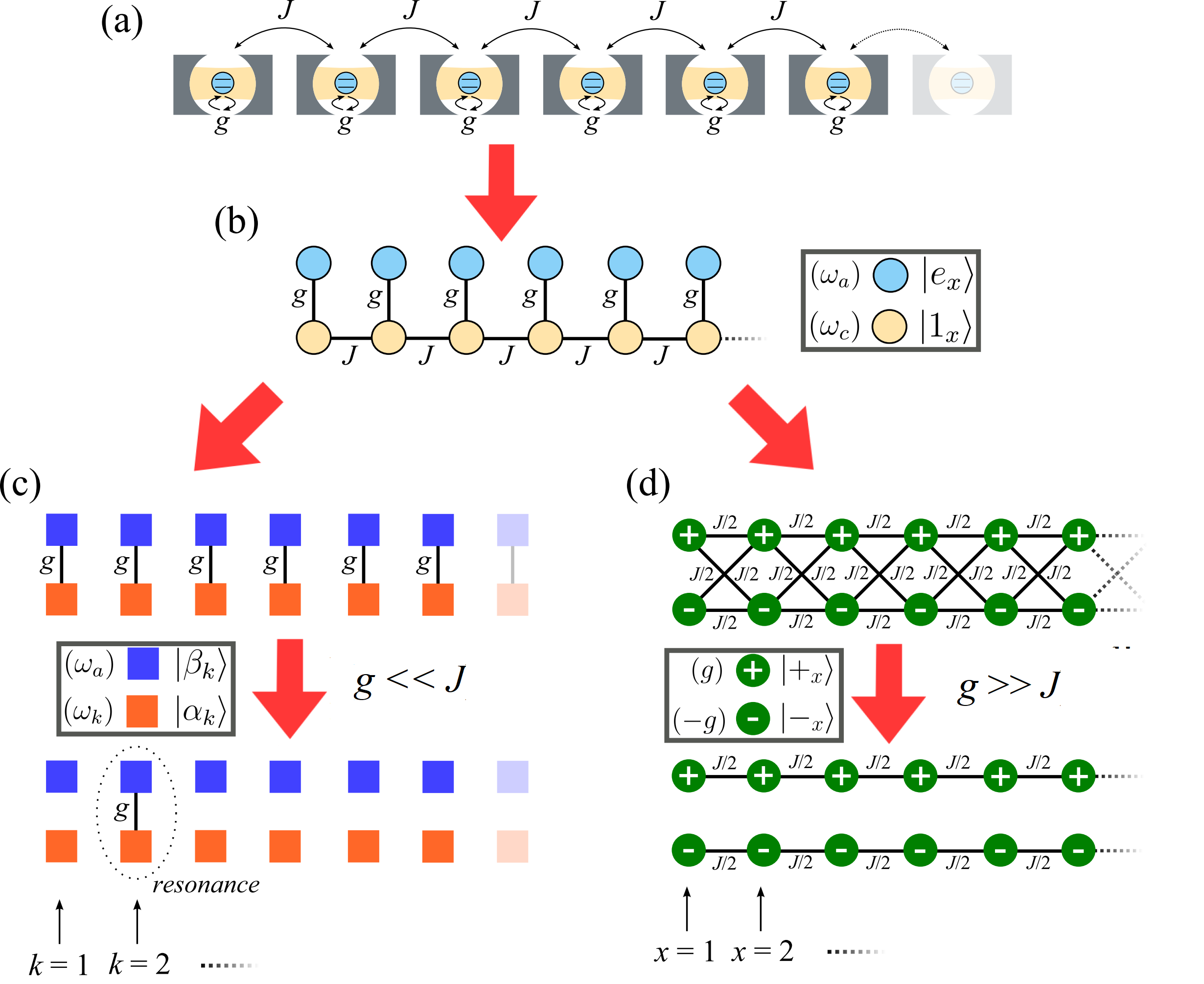
Figure 1: (Color online) State-graph structure of the JCH Hamiltonian describing a coupled-cavity system. (a) Sketch of an array featuring a uniform pattern of hopping rates $J$. Each cavity has frequency $\omega_{c}$ and is coupled to a two-level atom (or qubit) with frequency $\omega_{a}$ through a local atom-field interaction given by $g$. (b) In the single-excitation sector, the model is reduced to a tight-binding chain (with extra, vertically attached sites) where single-photon states ($\{\ket{1_{x}}\}$) spreads over the array and is eventually converted into atomic degrees of freedom ($\{\ket{e_{x}}\}$). (c) The JCH Hamiltonian may be expressed in terms of decoupled JC-like interactions between free-field normal modes $\{\ket{\alpha_{k}}\}$ and its atomic analog $\{\ket{\beta_{k}}\}$. In the weak atom-field coupling regime ($g\ll J$), proper tuning leads to a single resonant effective interaction (for $k=2$ in the example). (d) Another form of expressing the JCH Hamiltonian is in terms of polaritonic states $\{\ket{+_{x}},\ket{-_{x}}\}$ [see Eq. III]. The resulting double inter-connected array can be decoupled in the strong atom-field coupling regime ($g\gg J$) by dropping out fast rotating terms. In this particular case, we have a standard hopping-like Hamiltonian for each branch of polariton having exactly the same dispersion law of the embedded structure with the hopping intensity rescaled to $J/2$.

First, we recall that when the atom-field interaction strength $g$ and the atomic transition frequency $\omega_{a}$ are uniform across the array, Hamiltonian (2) can be rearranged as a sum of $N$ decoupled JC-like interactions, $H=\sum_{k}H_{k}$, in terms of normal modes, where Ogden et al. (2008); Makin et al. (2009); Ciccarello (2011); Almeida et al. (2016)

$$H_{k}=\omega_{k}\alpha_{k}^{\dagger}\alpha_{k}+\omega_{a}\beta_{k}^{\dagger}\beta_{k}+g(\alpha_{k}^{\dagger}\beta_{k}+\beta_{k}^{\dagger}\alpha_{k}),$$ (3)

and $\alpha_{k}^{\dagger}\equiv|\alpha_{k}\rangle\langle\emptyset|$ ($\beta_{k}^{\dagger}\equiv|\beta_{k}\rangle\langle\emptyset|$) is the field (atomic) normal-mode operator. In other words, $\{\ket{\alpha_{k}}\}$ is the set of $N$ eigenstates of the hopping (free-field) Hamiltonian, with eigenvalues $\{\omega_{k}\}$, each having the form $\ket{\alpha_{k}}=\sum_{x}v_{k,x}\ket{1_{x}}$. The atomic states $|\beta_{k}\rangle$ are set with the very same spatial profile (amplitudes) as their photonic counterpart, that is $\ket{\beta_{k}}=\sum_{x}v_{k,x}\ket{e_{x}}$ but all lying at the same frequency $\omega_{a}$. Although we are dealing with a uniform pattern of hopping rates, the above situation is valid regardless of the embedded adjacency matrix. Therefore, the model can be solved analytically once one knows the whole free-field spectral decomposition. Indeed, since the above Hamiltonian is a $2\times 2$ block-diagonal matrix indexed by $k$, its eigenstates are found to be Ciccarello (2011); Almeida et al. (2016)

$$\left|\psi_{k}^{\pm}\right>=A_{k}^{\pm}\left|\alpha_{k}\right>+B_{k}^{\pm}\left|\beta_{k}\right>,$$ (4)

where

$$A_{k}^{\pm}=\dfrac{2g}{\sqrt{(\Delta_{k}\pm\Omega_{k})^{2}+4g^{2}}},\,\,\,B_{k}^{\pm}=\dfrac{\Delta_{k}\pm\Omega_{k}}{\sqrt{(\Delta_{k}\pm\Omega_{k})^{2}+4g^{2}}},$$ (5)

$\Delta_{k}=\omega_{a}-\omega_{k}$ is the detuning between the atomic and the field normal-mode frequency, and $\Omega_{k}=\sqrt{\Delta_{k}^{2}+4g^{2}}$ is the corresponding vacuum Rabi frequency. The energy levels are given by

$$\varepsilon_{k}^{(\pm)}=\tfrac{1}{2}\,(\omega_{a}+\omega_{k}\pm\Omega_{k}).$$ (6)

The JCH Hamiltonian written in the form of effective JC interactions [see Eq. (3)] allows for a convenient visualization of the system’s behavior, as shown in Fig. 1(c). One of the most interesting features is the possibility of setting up a particular mode to trigger out a pair of dressed JC-like states [c.f. Eq. (4)]. This can be done in the weak atom-field coupling regime, $g\ll J$, upon a judicious tuning of the atomic frequency $\omega_{a}$. In order to see this, let us move on to the interaction picture,

$$H^{I}(t)=g\left(\sum_{k}\alpha_{k}^{\dagger}\beta_{k}e^{-i\Delta_{k}t}+\mathrm{H.c.}\right).$$ (7)

Setting $\omega_{a}$ in resonance with a given mode, say $k^{\prime}$, one of the terms becomes time-independent ($\Delta_{k^{\prime}}=0$) and considering $g\ll\{\Delta_{k\neq k^{\prime}}\}$, all the remaining terms become fast rotating and thus can be ignored. Going back to the Schrödinger picture, we are left with the effective Hamiltonian

$$H_{\mathrm{eff}}=H_{k^{\prime}}+\sum_{k\neq k^{\prime}}(\omega_{k}\alpha_{k}^{\dagger}\alpha_{k}+\omega_{a}\beta_{k}^{\dagger}\beta_{k}),$$ (8)

where the first term is given by Eq. (3). The above equation describes a single JC-like interaction taking place at mode $k^{\prime}$, spanning a pair of fully dressed states $\ket{\psi_{k^{\prime}}^{\pm}}$ [cf. Eq. (4)], with all the other atomic and field modes uncoupled. A schematic representation of this regime is shown in Fig. 1(c).

Within the weak coupling regime, if an atomic excitation is prepared somewhere along the array, say $\ket{\psi(0)}=\ket{e_{x_{0}}}$ , it may get stuck depending on the nature of the free-field spectrum and resonance conditions Makin et al. (2009); Ciccarello (2011); Almeida and Souza (2013); Almeida et al. (2016). In the off-resonant case, that is $\omega_{a}\neq\omega_{k}$ for all $k$, it is immediate to note that $\ket{\psi(t)}=e^{-iHt}\ket{\psi(0)}=e^{-i\omega_{a}t}\ket{e_{x_{0}}}$ and so the atomic excitation indeed freezes at the initial cavity $x_{0}$. Now, if $\omega_{a}$ is put in narrow resonance with a given (nondegenerate) mode $k^{\prime}$ thereby setting up a JC-like interaction between this mode and its atomic counterpart, the evolved atomic coefficients read

$$c_{a,x}(t)=e^{-i\omega_{a}t}\left[\sum_{k\neq k^{\prime}}v_{k,x}v_{k,x_{0}}^{*}+\cos{(gt)v_{k^{\prime},x}v_{k^{\prime},x_{0}}^{*}}\right],$$ (9)

and as $\sum_{k}v_{k,x}v_{k,x_{0}}^{*}=1$ ($=0$) for $x=x_{0}$ ($x\neq x_{0}$) due to orthonormality, the return probability

$$p_{a,x_{0}}\equiv|c_{a,x_{0}}(t)|^{2}=[1+|v_{k^{\prime},x_{0}}|^{2}(\cos{gt}-1)]^{2}.$$ (10)

In other words, the amount of information released by the initial excitation ultimately depends on the overlap between $\ket{\beta_{k^{\prime}}}$ and $\ket{e_{x_{0}}}$. For a uniform array, which is our case, the free-field spectrum consists of plane waves of the form $v_{k,x}\propto\sin{(kx)}$, with $k=\pi m/(N+1)$ and $m=1,\ldots,N$, and so the overlap should be small enough to retain most of the amplitude. Still, for finite $N$ some amount of atomic probability periodically flows out of the initial state reaching the other atomic states in phase as

$$p_{a,x}=|v_{k^{\prime},x}v_{k^{\prime},x_{0}}^{*}|^{2}(\cos{gt}-1)^{2}$$ (11)

for $x\neq x_{0}$.

Taking the other limit, that is when we increase $g/J$ until reaching the strong atom-field coupling regime Makin et al. (2009); Almeida and Souza (2013), every normal mode becomes fully dressed and the corresponding eigenstates effectively take the form $\ket{\psi_{k}^{\pm}}=(\ket{\alpha_{k}}\pm\ket{\beta_{k}})/\sqrt{2}$. These are polaritons that form two single-particle dispersion branches having the very same structure as of an embedded array with the hopping scale redefined by $J/2$ [see Eq. (6)]. A much better way to visualize this is by rewriting the JCH Hamiltonian, Eq. (2) in terms of local polaritonic operators $P_{x}^{(n,\pm)}\equiv\ket{\emptyset}_{x}\bra{n\pm}$ Angelakis et al. (2007). Dropping out terms with $n\neq 1$ the Hamiltonian becomes (recall we set $\omega_{c}=0$)

$$H =g\sum_{x=1}^{N}\left(P_{x}^{(+)\dagger}P_{x}^{(+)}-P_{x}^{(-)\dagger}P_{x}^{(-)}\right)$$

$$-\dfrac{J}{2}\sum_{x=1}^{N-1}\left(P_{x}^{(+)\dagger}P_{x+1}^{(+)}+P_{x}^{(-)\dagger}P_{x+1}^{(-)}\right.$$

$$\left.+P_{x}^{(+)\dagger}P_{x+1}^{(-)}+P_{x}^{(-)\dagger}P_{x+1}^{(+)}+\mathrm{H.c.}\right),$$ (12)

where $P_{x}^{(\pm)}\equiv P_{x}^{(1,\pm)}$ for brevity. The above Hamiltonian is equivalent to a double tight-binding array connected to each other through the hopping terms that exchange between even ($\ket{+}_{x}$) and odd ($\ket{-}_{x}$) polaritons [see Fig. 1(d)]. This can be further simplified in the strong coupling regime ($g\gg J$), where both chains become effectively decoupled Angelakis et al. (2007); Makin et al. (2009), i.e., those inter-converting terms are fast rotating and can be dropped out. It is worth mentioning that the even and odd polaritonic operators obey, each, the same algebra as the spin$-1/2$ ladder operators. Therefore, in this regime, the JCH Hamiltonian effectively describes a $XY$ spin chain with spin up (down) corresponding to the presence (absence) of polaritons Angelakis et al. (2007); Bose et al. (2007).

In such strong atom-field coupling scenario the dynamics of the atomic excitation mimics that of a single particle propagating along either of the uncoupled effective chains (it spreads out ballistically in a uniform chain) with hopping constant $J/2$, the only difference being that it is continuously converted back and forth to a photonic state at rate $g$ Makin et al. (2009). Time-evolved atomic coefficients in this case read

$$c_{a,x}(t)=\cos{gt}\sum_{k}e^{-i\frac{\omega_{k}}{2}t}v_{k,x}v_{k,x_{0}}^{*}.$$ (13)

Also note in Fig. 1(d) that if the system is initialized in an even (odd) polariton state, the odd (even) counterpart will not take part in the dynamics.

IV Entanglement properties

Now that we have made an overall analysis of the two main limiting regimes of the JCH model, we are to track the entanglement over time between atomic and photonic degrees of freedom via the von Neumann entropy as well as between pairs of atoms via the concurrence. Those measures are introduced next.

IV.1 Entanglement measures

The single-excitation subspace is spanned by $\{\ket{1_{i}},\ket{e_{i}}\}$ so that a general state can be written as

$$\ket{\psi}=\sum_{i=1}^{N}\left(c_{f,i}\ket{1_{i}}+c_{a,i}\ket{e_{i}}\right),$$ (14)

where $c_{f,x}$ and $c_{a,x}$ are the field and atomic coefficients, respectively. In the density-operator formalism, we have

$$\rho=\ket{\psi}\bra{\psi}= \sum_{i=1}^{N}\sum_{j=1}^{N}(c_{f,i}c_{f,j}^{*}\ket{1_{i}}\bra{1_{j}}+c_{f,i}c_{a,j}^{*}\ket{1_{i}}\bra{e_{j}}$$

$$+c_{a,i}c_{f,j}^{*}\ket{e_{i}}\bra{1_{j}}+c_{a,i}c_{a,j}^{*}\ket{e_{i}}\bra{e_{j}}).$$ (15)

Now, tracing out the cavity (field) modes, $\rho_{a}=\mathrm{Tr}_{f}[\rho]$, we obtain

$$\rho_{a}=\sum_{i=1}^{N}|c_{f,i}|^{2}\ket{\Downarrow}\bra{\Downarrow}+\sum_{i=1}^{N}\sum_{j=1}^{N}c_{a,i}c_{a,j}^{*}{\sigma}_{i}^{+}\ket{\Downarrow}\bra{\Downarrow}{\sigma}_{j}^{-},$$ (16)

where $\ket{\Downarrow}\equiv\ket{g}_{1}\ldots\ket{g}_{N}$.

Note that, in general, $\rho_{a}$ is a mixed state and thus the atomic component, as a whole, is said to be entangled with the photonic subsystem. The diagonal form of $\rho_{a}$ has only two entries, $\Pi_{f}\equiv\sum_{i}|c_{f,i}|^{2}$ and $\Pi_{a}\equiv\sum_{i}|c_{a,i}|^{2}$, namely the total photonic and atomic probabilities, respectively. Since $\ket{\psi}$ is a pure state, we can evaluate the amount of entanglement between two partitions through the von Neumann entropy. For the, say, atomic component,

$$S[\rho_{a}]=-\mathrm{Tr}\rho_{a}\mathrm{log}_{2}\rho_{a}=-\Pi_{a}\mathrm{log}_{2}\Pi_{a}-(1-\Pi_{a})\mathrm{log}_{2}(1-\Pi_{a}),$$ (17)

which gives 0 (1) for a fully separable (entangled) state. Note that the entropy reaches its maximum for $\Pi_{f}=\Pi_{a}=1/2$, that is $S_{\mathrm{max}}=-\mathrm{log}_{2}(1/2)=1$.

To evaluate bipartite entanglement between the atoms we choose a pair of sites, say, $i$ and $j$ and further trace out the rest of them from $\rho_{a}$ [Eq. (16)] to obtain a four dimensional reduced matrix spanned in the basis $\{\ket{gg},\ket{ge},\ket{eg},\ket{ee}\}$,

$$\rho_{i,j}=\begin{bmatrix}1-|c_{a,i}|^{2}-|c_{a,j}|^{2}&0&0&0\\ 0&|c_{a,i}|^{2}&c_{a,i}c_{a,j}^{*}&0\\ 0&c_{a,j}c_{a,i}^{*}&|c_{a,j}|^{2}&0\\ 0&0&0&0\end{bmatrix}.$$ (18)

Despite the fact that it is not straightforward to evaluate the entanglement of a mixed state, a simple expression does exist for an arbitrary state of two qubits. The so-called concurrence is defined by Wootters (1998)

$$C(\rho_{i,j})=\mathrm{max}\{0,\sqrt{\lambda_{1}}-\sqrt{\lambda_{2}}-\sqrt{\lambda_{3}}-\sqrt{\lambda_{4}}\},$$ (19)

where $\{\lambda_{i}\}$ are decreasing eigenvalues, of the matrix $\rho_{i,j}\tilde{\rho}_{i,j}$, with

$$\tilde{\rho}_{AB}=(\sigma_{y}\otimes\sigma_{y})\rho_{AB}^{*}(\sigma_{y}\otimes\sigma_{y})$$ (20)

and $\rho_{i,j}^{*}$ being the complex conjugate of $\rho_{i,j}$, and $\sigma_{y}$ the Pauli operator. For a separable (fully-entangled) state $C=0$ ($C=1$). Evaluating for Eq. (18), we get

$$C_{i,j}\equiv C\left(\rho_{i,j}\right)=2|c_{a,i}c_{a,j}^{*}|=2|\langle e_{i}|\psi\rangle\langle\psi|e_{j}\rangle|.$$ (21)

IV.2 Time evolution

The protocol starts with a single atomic excitation prepared in the middle of the coupled-cavity system and we let it evolve naturally as $\ket{\psi(t)}=e^{-iHt}\ket{e_{x_{0}}}$, with $x_{0}=\frac{N+1}{2}$ and $N$ being odd so as to have a mode at the center of the band. We keep $\omega_{a}=0$ henceforth. Note that this triggers a JC-like interaction between atomic and field modes at that level when in the weak-coupling regime, as discussed in the previous section. Also note that [cf. Eq. (9)] $v_{k,\frac{N+1}{2}}\propto\sin{\pi m/2}=0$ for even $m$. As the resonance is set at the center of the band, $m=(N+1)/2$ must be an odd number, otherwise there is no propagation when $g\ll J$.

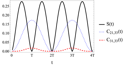
Figure 2: (Color online) Exact time evolution of the atom-field von Neumann entropy $S$ and atomic concurrences $C_{x_{0},33}$, $C_{31,33}$, for $\ket{\psi(t=0)}=\ket{e_{x_{0}}}$ with $x_{0}=21$ on a uniform coupled-cavity array featuring $N=41$ sites operating in the weak coupling regime with $g=10^{-3}J$ and $\omega_{a}=\omega_{c}=0$. The entropy oscillates with period $T=\pi/g$.

Given the fact that the atomic wavefunction can only spread out if mediated by the field, generation of entanglement between pairs of atoms must be preceded by the development of atom-field correlations. We are now to see how this goes for both limiting interaction regimes. The exact entropy dynamics for the weak-coupling regime ($g\ll J$) is depicted in Fig. 2 alongside concurrence for two distinct pairs of atoms. The total atomic probability $\Pi_{a}(t)=1-|v_{k^{\prime},x_{0}}|^{2}\sin^{2}(gt)$ and thus the entropy evolves with period $T=\pi/g$, half that of the return probability in Eq. (10). So, two entropy cycles cover (from the beginning) the release of energy from $\ket{e_{x_{0}}}$ to the photonic degrees of freedom, followed by excitation of the remaining atomic states [see Eq. (11)] at $t=T$ (when $S=0$), ending up with full recovery of the initial state at $t=2T$ via a second transition through the photonic mode. Atomic concurrences set along within the same timescale, reaching its maximum at times $t=T,3T,5T,\ldots$ in phase, as already implied in Eq. (11). In general, it is crucial to highlight that degree of entropy generation, as well as the precise timing of the maximum concurrence are governed by the overlap $v_{k^{\prime},x_{0}}$ since communication between atomic and photonic degrees of freedom in the weak coupling regime involves exchange between $\ket{\alpha_{k^{\prime}}}$ and $\ket{\beta_{k^{\prime}}}$ at a single level $k^{\prime}$, rather than over the full spectrum. Another feature to note in Fig. 2 – also by a careful inspection of Eq. (9) – is that the concurrence involving the atom located at the initial site $x_{0}$ overcomes entanglement between any other pair (Fig. 2 shows that for two representative pairs). This is due to the spectral profile of the uniform coupled-cavity array for it restricts the flow out of $\ket{e_{x_{0}}}$ thereby leaving the remaining cavities with limited resources to establish atomic entanglement, especially for larger $N$.

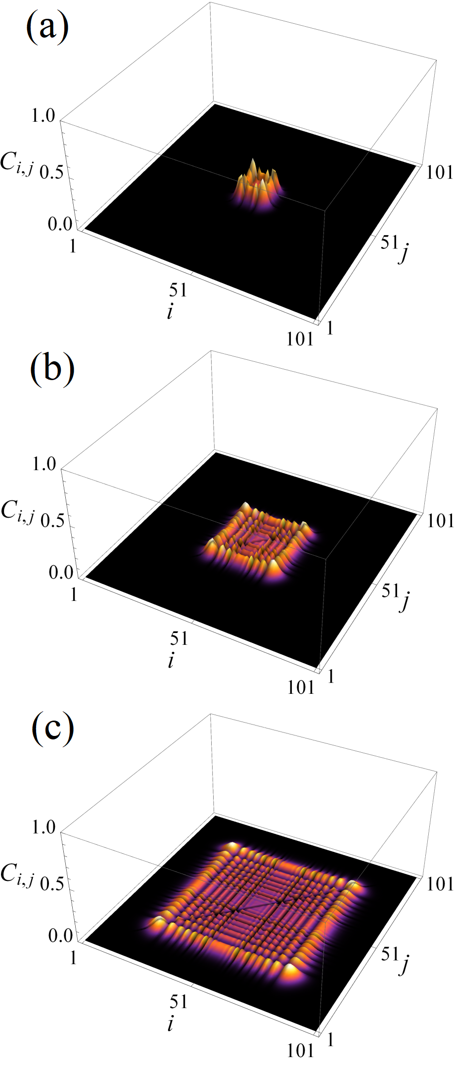
Figure 3: (Color online) Snapshots of the atomic concurrence distribution $C_{i,j}(t)$ in the strong coupling regime for (a) $t=2000\pi/g$, (a) $t=5000\pi/g$, and (c) $t=10000\pi/g$, with $g=10^{3}J$, such that $\Pi_{a}(t)=\cos^{2}(gt)=1$ (thus $S(t)=0$). The system consists of $N=101$ coupled cavities with the initial state being $\ket{\psi(t=0)}=\ket{e_{51}}$ and $\omega_{a}=\omega_{c}=0$ and results are exact as obtained directly from Hamiltonian (2). Note that the atomic wavefunction propagates at rate $J/2$ and thus the front pulse roughly advances a site per $J^{-1}$ elapsed time.

Moving on to the the strong coupling regime ($g\gg J$), we get a whole different picture. Now, there is no special mode triggering the dynamics. All the modes are involved and atomic degrees of freedom are completely mixed with their photonic analogs. Assisted by photonic scattering, the initial atomic excitation spreads out ballistically at rate $J/2$, as $\ket{e_{x_{0}}}$ is a superposition of even and odd polaritons, both spanning the uncoupled effective chains seen in Fig. 1(d). As it propagates, the atomic wavefunction is constantly mirrored back and forth to its photonic form in a much faster timescale. In this limit, the entropy is fed with total atomic probability $\Pi_{a}(t)=\cos^{2}(gt)$, implying that $S(t)$ reaches maximum at times $t=m\pi/(4g)$ for odd $m$ (that is when $\Pi_{a}(t)=1/2$). Note that the above property is general in that it holds for any size $N$ and hopping scheme, with the resulting atomic dynamics always obeying the underlying spectral properties of the coupled-cavity array, as long as $g$ is larger than the free-field band width as well as $\omega_{a}$. Therefore, given that entropy generation is local, generation of atomic entanglement is ultimately driven by wave dispersion. Figure 3 shows some snapshots of the concurrence distribution at times when $\Pi_{a}(t)=1$ to get the most of $C_{i,j}$. As one should expect, entanglement is well distributed throughout the array as it evolves, with stronger correlations taking place within each front pulse as well as between them.

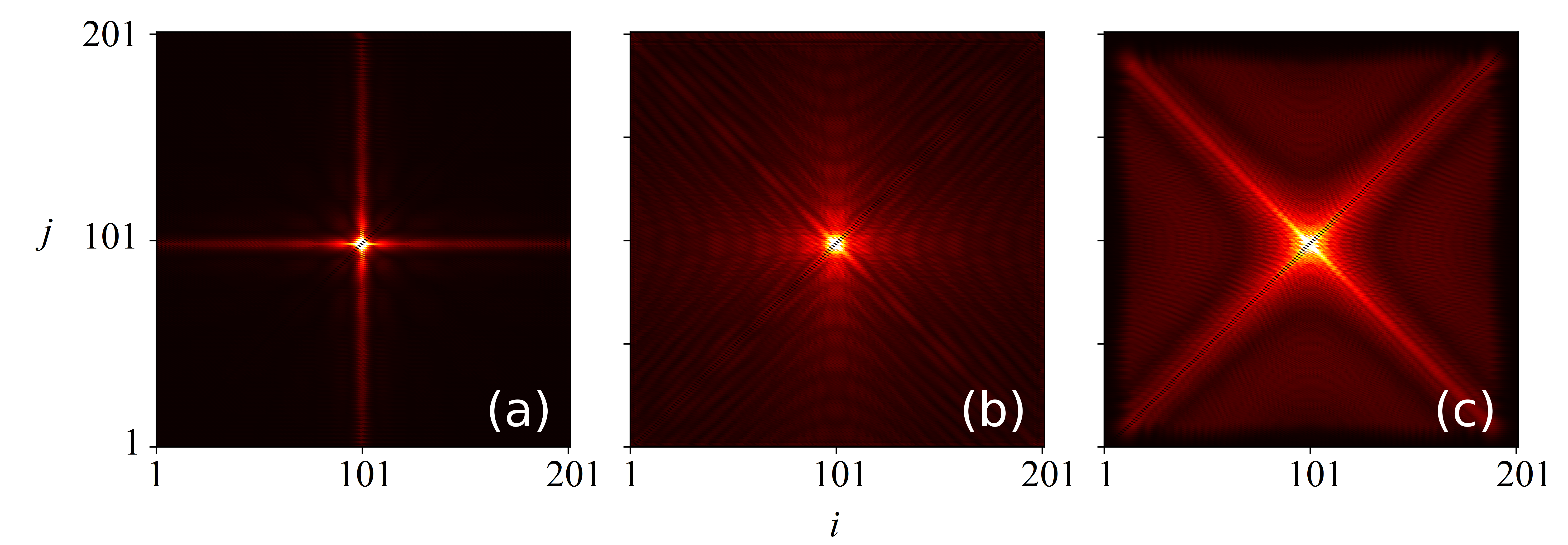
Figure 4: (Color online) Maximum concurrence $C_{i,j}(t)$ between all pairs of atoms recorded within time interval $tJ\in[0,90]$ for three distinct regimes represented by (a) $g=0.1J$, (b) $g=1.5J$, and (c) $g=10J$, considering $N=201$ cavities and $\ket{\psi(t=0)}=\ket{e_{101}}$. The time window was chosen so that the wavefunction did not reach the boundaries in (c). Color map goes from dark to bright as $C_{i,j}(t)\in[0,0.25)$.

Finally, to get a better glance over the spatial distribution of atomic entanglement, in Fig. 4 we display the maximum concurrence recorded within a fixed time interval for all $C_{i,j}$ ($i\neq j$) and covering three different regimes. In the weak coupling scenario, as a single atomic excitation prepared above the ground state of a uniform coupled-cavity array undergoes a trapping mechanism Makin et al. (2009); Ciccarello (2011); Almeida et al. (2016), it pairs up with each of the remaining atoms to produce the entanglement pattern we see in Fig. 4(a). In this situation, we shall remember that entanglement does not spread out from the center of the array [as in Fig. 3]; it is generated all at once as the entropy dynamics involves resonant interaction between atomic and photonic delocalized modes (cf. Fig. 2). We observe that such spatial pattern similar to that of disordered chains reported in Ref. Almeida et al. (2017), what is very interesting as our array is fully uniform. It means that the atomic trapping mechanism can be thought as a sort of interaction-induced localization.

Setting up a moderate interaction strength ($g\sim J$), the entanglement distribution in Fig. 4(b) does not seem to display a very definite pattern but it marks a crossover to the strong coupling regime shown in Fig. 4(c). This one is highlighted by the onset of stronger correlations between neighboring atoms as well as between atoms equidistant from the center of the array, as already suggested by Fig. 3. As a full band of extended states begins to take over the dynamics as $g$ is increased, the initial atomic excitation rapidly communicates with the photonic degrees of freedom locally and spreads out simulating the dynamics of single photon in a atom-free coupled-cavity array with $J$ replaced by $J/2$ in the limit $g\gg J$. Those maxima in Fig. 4(c) are thus recorded when the front pulse of the atomic wavefunction passes by Almeida et al. (2017).

V Concluding remarks

We have studied entanglement generation and its spatial distribution control over a 1D uniform coupled-cavity array described by the JCH Hamiltonian in the single-excitation sector. We carried out detailed analytical calculations for two limiting regimes so as to gain intuition over how photonic and atomic degrees of freedom are combined when put to interact via the JC Hamiltonian.

With all that set, we moved on to study entanglement generation via time evolution of a single atomic excitation prepared above the vacuum (ground) state. We focused on the von Neumann entropy between atomic and field states and the concurrence between pairs of atoms. We found that, in the weak coupling regime ($g\ll J$), entropy generation follows the same timescale as that of concurrence and depends directly on the likelihood of energy release from the emitter located at the initial cavity – which, in turn, depends on the resonant field mode –, thus being crucial to make resources available to the other atoms to build up correlations. Because of the atomic trapping behavior, entanglement between the initial atom and the remaining ones prevails over that involving any other pair. This sort of interaction-induced localization occurring in the weak coupling regime is certainly worth to be further investigated in other scenarios, such as beyond the single-excitation subspace where the photon-blockade sets in. Things should also become more involved when considering, for instance, complex networks Almeida and Souza (2013) and other lattices with unique topological features Ciccarello (2011); Almeida et al. (2016), where localized modes are built-in.

In the strong coupling regime ($g\gg J$), entanglement dynamics is more straightforward as the entropy oscillates (now between minimum and maximum) much faster than the actual propagation of the atomic wavefunction, meaning that entropy generation is strictly due to local interactions, differently from the weak coupling limit. Atomic concurrence then builds up depending on the dispersion profile of the embedded array at rate $J/2$. A uniform one entails ballistic spreading and so the amplitudes are concentrated within the front pulse. Higher degrees of pairwise entanglement are then to be found in between nearest-neighbor atoms and between them and their equidistant counterpart at the other side of the array in respect to its center.

Although we found that long-distance atomic entanglement becomes weaker due to dispersive effects of the array itself, it may be distilled into pure singlets Horodecki et al. (1998), to be used in, e.g., quantum teleportation protocols. The natural dynamics of the JCH Hamiltonian may thus be harnessed to generate entanglement between distant nodes in hybrid light-matter quantum network architectures Kimble (2008); Ritter et al. (2012).

References

- Horodecki et al. (2009) R. Horodecki, P. Horodecki, M. Horodecki, and K. Horodecki, Rev. Mod. Phys. 81, 865 (2009).
- Amico et al. (2008) L. Amico, R. Fazio, A. Osterloh, and V. Vedral, Rev. Mod. Phys. 80, 517 (2008).
- Vidal et al. (2003) G. Vidal, J. I. Latorre, E. Rico, and A. Kitaev, Phys. Rev. Lett. 90, 227902 (2003).
- Osterloh et al. (2002) A. Osterloh, L. Amico, G. Falci, and R. Fazio, Nature 416, 608 (2002).
- Bennett et al. (1993) C. H. Bennett, G. Brassard, C. Crépeau, R. Jozsa, A. Peres, and W. K. Wootters, Phys. Rev. Lett. 70, 1895 (1993).
- Ekert (1991) A. K. Ekert, Phys. Rev. Lett. 67, 661 (1991).
- Gisin et al. (2002) N. Gisin, G. Ribordy, W. Tittel, and H. Zbinden, Rev. Mod. Phys. 74, 145 (2002).
- Bennett and Wiesner (1992) C. H. Bennett and S. J. Wiesner, Phys. Rev. Lett. 69, 2881 (1992).
- DiVincenzo (1995) D. P. DiVincenzo, Science 270, 255 (1995).
- Cirac et al. (1997) J. I. Cirac, P. Zoller, H. J. Kimble, and H. Mabuchi, Phys. Rev. Lett. 78, 3221 (1997).
- Kimble (2008) H. J. Kimble, Nature 453, 1023 (2008).
- Schoelkopf and Girvin (2008) R. J. Schoelkopf and S. M. Girvin, Nature 451, 664 (2008).
- Ritter et al. (2012) S. Ritter, C. Nölleke, C. Hahn, A. Reiserer, A. Neuzner, M. Uphoff, M. Mücke, E. Figueroa, J. Bochmann, and G. Rempe, Nature 484, 195 (2012).
- Nölleke et al. (2013) C. Nölleke, A. Neuzner, A. Reiserer, C. Hahn, G. Rempe, and S. Ritter, Phys. Rev. Lett. 110, 140403 (2013).
- Reiserer et al. (2014) A. Reiserer, N. Kalb, G. Rempe, and S. Ritter, Nature 508, 237 (2014).
- Reiserer and Rempe (2015) A. Reiserer and G. Rempe, Rev. Mod. Phys. 87, 1379 (2015).
- Greentree et al. (2006) A. D. Greentree, C. Tahan, J. H. Cole, and L. C. L. Hollenberg, Nat. Phys. 2, 856 (2006).
- Angelakis et al. (2007) D. G. Angelakis, M. F. Santos, and S. Bose, Phys. Rev. A 76, 031805(R) (2007).
- Tomadin and Fazio (2010) A. Tomadin and R. Fazio, J. Opt. Soc. Am. B 27, A130 (2010).
- Rossini and Fazio (2007) D. Rossini and R. Fazio, Phys. Rev. Lett. 99, 186401 (2007).
- Almeida et al. (2016) G. M. A. Almeida, F. Ciccarello, T. J. G. Apollaro, and A. M. C. Souza, Phys. Rev. A 93, 032310 (2016).
- Hartmann et al. (2008) M. Hartmann, F. Brandão, and M. Plenio, Laser & Photonics Reviews 2, 527 (2008).
- Amico et al. (2004) L. Amico, A. Osterloh, F. Plastina, R. Fazio, and G. Massimo Palma, Phys. Rev. A 69, 022304 (2004).
- Almeida et al. (2017) G. M. A. Almeida, F. A. B. F. de Moura, T. J. G. Apollaro, and M. L. Lyra, Phys. Rev. A 96, 032315 (2017).
- Fukuhara et al. (2015) T. Fukuhara, S. Hild, J. Zeiher, P. Schauß, I. Bloch, M. Endres, and C. Gross, Phys. Rev. Lett. 115, 035302 (2015).
- Makin et al. (2009) M. I. Makin, J. H. Cole, C. D. Hill, A. D. Greentree, and L. C. L. Hollenberg, Phys. Rev. A 80, 043842 (2009).
- Ciccarello (2011) F. Ciccarello, Phys. Rev. A 83, 043802 (2011).
- Jaynes and Cummings (1963) E. T. Jaynes and F. W. Cummings, Proceedings of the IEEE 51, 89 (1963).
- Almeida and Souza (2013) G. M. A. Almeida and A. M. C. Souza, Phys. Rev. A 87, 033804 (2013).
- Ogden et al. (2008) C. D. Ogden, E. K. Irish, and M. S. Kim, Phys. Rev. A 78, 063805 (2008).
- Bose et al. (2007) S. Bose, D. G. Angelakis, and D. Burgarth, J. Mod. Opt. 54, 2307 (2007).
- Wootters (1998) W. K. Wootters, Phys. Rev. Lett. 80, 2245 (1998).
- Horodecki et al. (1998) M. Horodecki, P. Horodecki, and R. Horodecki, Phys. Rev. Lett. 80, 5239 (1998).