Solution Path Algorithm for Twin Multi-class Support Vector Machine

Abstract

The twin support vector machine and its extensions have made great achievements in dealing with binary classification problems. However, it suffers from difficulties in effective solution of multi-classification and fast model selection. This work devotes to the fast regularization parameter tuning algorithm for the twin multi-class support vector machine. Specifically, a novel sample data set partition strategy is first adopted, which is the basis for the model construction. Then, combining the linear equations and block matrix theory, the Lagrangian multipliers are proved to be piecewise linear w.r.t. the regularization parameters, so that the regularization parameters are continuously updated by only solving the break points. Next, Lagrangian multipliers are proved to be 1 as the regularization parameter approaches infinity, thus, a simple yet effective initialization algorithm is devised. Finally, eight kinds of events are defined to seek for the starting event for the next iteration. Extensive experimental results on nine UCI data sets show that the proposed method can achieve comparable classification performance without solving any quadratic programming problem.

1 Introduction

As a machine learning method for pattern classification, the well-known support vector machine (SVM) by solving a quadratic programming problem (QPP) has shown the great prospect and excellent generalization performance after decades of evolutionary development since it was proposed by Cortes & Vapnik (1995). Based on the structural risk minimization principle and Vapnik-Chervonenkis dimensional theory in statistical learning theory, SVM has been widely used in data mining (Luo et al., 2020; Vaidya et al., 2008), knowledge discovery (Hsieh & Yeh, 2011; Zhang et al., 2014), clustering (Bai et al., 2019; Lee & Lee, 2005) and other fields (Yang et al., 2015; Sun, 2011; Xie & Sun, 2020; Sun et al., 2018; Sun & Xie, 2015; Li et al., 2021). To enhance its predictive performance and computational efficiency (Hu et al., 2013), the twin SVM (TSVM) has been developed by Jayadeva et al. (2007), which generates two non-parallel hyperplanes where each class is close to one and away from the other by solving a pair of smaller sized QPPs (Xie et al., 2018).

It is well-known that TSVM (Jayadeva et al., 2007) is initially designed for the binary classification problem. Since most real-life applications are related to multi-class classifications (Chen & Wu, 2017) such as activity recognition, speaker identification and text categorization, extending it to multi-classification problems is of great significance. Based on this, researchers have proposed many strategies, where “one-versus-one” (OVO), “one-versus-rest” (OVR) and “one-versus-one-versus-rest” (OVOVR) are three of the most commonly used methods (KreBel, 1999; Xie et al., 2013; Xu et al., 2013; Wang & Zhang, 2021). These different strategies have been reviewed by Ding et al. (2019). For example, Xu et al. (2013) have proposed a multi-class classification algorithm with the OVOVR structure and produced better forecasting results than other strategies. Furthermore, some two-class techniques are often not helpful when being directly applied to the multi-class problem (Zhou & Liu, 2005), the OVOVR strategy has received much attention (Pang et al., 2018; Pan et al., 2017; Pang et al., 2019). For example, Pan et al. (2017) have designed safe screening rules for accelerating the classification of TSVM. To extend it to twin multi-class SVM, Pang et al. (2018) have proposed a safe sample elimination rule for accelerating the classification. These methods can effectively accelerate the classification, whereas, efficiently obtaining the optimal regularization parameters is not involved. In this work, we aim to explore the efficient model selection w.r.t. the regularization parameters for twin multi-class SVM based on the OVOVR strategy.

To get the optimal regularization parameter, it is very time-consuming for the traditional grid search method, especially for multi-parameter models. Since Hastie et al. (2004) have proposed the entire regularization path for SVM, exploring the solution path algorithm has become one of the most efficient methods to handle the efficient model selection problem for SVM and its extensions. As can be seen in (Hastie et al., 2004), the solution path algorithm aims to establish the piecewise linear relationships between the regularization parameters and the Lagrangian multipliers. Since then, researchers have also proposed some methods to explore the solution path algorithm for TSVMs. For example, a new solution-path approach for the pinball TSVM has been proposed by Yang et al. (2018) and we also have proposed a fast regularization parameter tuning algorithm for TSVM (Zhou et al., 2022). However, the entirely regularized path algorithm for multi-class problems is much more difficult due to their intrinsic complexity. Thus, there have not been the entirely regularized solution path algorithm for twin multi-class SVM with the OVOVR structure. The reason is that the involved relationships between the regularization parameters and Lagrangian multipliers are quite complex. On the one hand, a simple yet effective initialization algorithm is hard to design. On the other hand, there are many complicated cases to consider for the OVOVR structure, so designing an efficient updating strategy is not easy. To address these problems, we propose an efficient regularized solution path algorithm for twin multi-class SVM.

In this work, twin multi-class SVM with the OVOVR strategy is transformed into two sub optimization models and the corresponding solution path algorithm is then proposed. Specifically, a novel sample data set partition strategy is first adopted, which is the basis for the model construction. Then, combining the linear equations and block matrix theory, the Lagrangian multipliers are proved to be piecewise linear w.r.t. the regularization parameters, so that the regularization parameters are continuously updated by only solving the break points. Next, Lagrangian multipliers are proved to be 1 as the regularization parameter approaches infinity, thus, a simple yet effective initialization algorithm is devised. Finally, eight kinds of events are defined to seek for the starting event for the next iteration. Extensive experimental results on several UCI data sets show that the proposed algorithm can achieve comparable classification performance without solving any quadratic programming problem. Code will be available at https://github.com/ZhouKanglei/TwinMultiPath.

The main contributions of this work are summarized as follows:

1. A novel sample set partition strategy is adopted and the Lagrangian multipliers of the twin multi-class support vector machine are proved to be piecewise linear w.r.t. the regularization parameters.

2. Eight kinds of events are defined and the entire solution path algorithm is proposed, in which the regularization parameters are continuously updated by only solving the break points.

3. Lagrangian multipliers are proved to be 1 as the regularization parameter approaches infinity and a simple initialization algorithm is presented, thus extending the search space of the regularization parameter to $(0,+\infty)$.

The rest of this work is structured: Section 2 briefly reviews the related work. Section 3 reviews the basic concept of TSVM. Details of the solution path algorithm for TSVM are introduced in Section 4. Section 5 shows a lot of experimental results. The conclusions of the whole paper are drawn in Section 6.

2 Related Work

In this section, we briefly review different TSVM extensions, multi-classification strategies for TSVM and solution path algorithms, respectively.

2.1 TSVM and Extensions

In the last two decades, significant research achievements have been made on TSVM, including the least squares TSVM (LSTSVM), weighted TSVM (WTSVM), projection TSVM (PTSVM), etc.

In 2009, Kumar & Gopal (2009) have presented LSTSVM, which introduces the concept of proximal SVM (PSVM) to the original problem of TSVM. Since only two linear equations are considered to obtain the result, the solution speed is improved a lot instead of solving two QPPs with constraints. Based on LSTSVM, many researchers have proposed different improved versions (Tanveer et al., 2016; Xu et al., 2015; de Lima et al., 2018). To solve the semi-positive definite problem in LSTSVM, which only satisfies the empirical risk minimization, Tanveer et al. (2016) have designed a robust energy-based LSTSVM. This method uses the energy model to solve the problem of imbalanced sample data and overcomes the influence of outliers and noise. Xu et al. (2015) have applied the prior structure information of the data to LSTSVM and constructed the structural LSTSVM. Due to the inclusion of data distribution information in the module, it has good generalization performance and short time consumption.

In 2012, based on local information, Ye et al. (2012) have proposed a WTSVM to alleviate the problem that similar information between any two data points in the same class cannot be utilized in TSVM. To reduce the influence of noise, Li et al. (2017) have proposed a new weighting mechanism based on LSTSVM. Xu (2016) has developed K-nearest neighbor (KNN)-based weighted multi-class TSVM, where the weight matrix is introduced into the objective function to explore the local information in the class, and two weight vectors are introduced into the constraint condition to find the inter-class information.

In 2011, Chen et al. (2011) have proposed PTSVM. The idea is to find two projection directions, each one corresponds to a projection direction. The algorithm recursively generates multiple projection axes for each class, which overcomes the problem of singular values and improves the performance of the algorithm. Furthermore, Xie & Sun (2014) have presented multi-view Laplacian TSVM by combining it with semi-supervised learning. Tomar & Agarwal (2015) have proposed the multi-class classification of LSTSVM by extending it to the contract state of multi-class classification. Wang et al. (2018) have developed an improved $\rho$-twin bounded SVM, which can effectively avoid the problem of matrix irreversibility in solving dual problems and has a strong generalization ability in processing large-scale data sets.

2.2 Multi-classification Strategies

To generalize the standard TSVM to the multi-classification problems (Weston & Watkins, 1999; Crammer & Singer, 2002), researchers have proposed many classification strategies such as OVO, OVR, OVOVR, all-together, etc.

KreBel (1999) has adopted the OVO classification strategy to establish a classifier between any two categories of samples. For the sample set with $K(K\geq 3)$ categories, $K(K-2)/2$ binary classification classifiers need to be constructed. And the category of the sample is determined according to its maximum vote (Hsu & Lin, 2002). Obviously, the disadvantage of this classifier is that the rest samples are not considered. In 2008, Cong et al. (2008) combined the OVR strategy with TSVM to achieve efficient speaker recognition. In 2013, Xie et al. (2013) proposed a novel OVR TSVM for the multi-class classification problem and analyzed its efficiency theoretically. For the OVR TSVM, by constructing $K$ binary classifiers, the $i$-th sample and the remaining samples can be distinguished by the $i$-th classifier. For unknown samples, they can be classified into the category with the maximum confidence w.r.t. the decision function. However, this method ignores the class imbalance problem. By combining the above strategies, the OVOVR TSVM, termed as Twin-KSVC, is proposed by Xu et al. (2013), which can yield better classification accuracy in comparison with other structures. Since then, this OVOVR structure has attracted much attention by researchers (Xu, 2016; Pang et al., 2018, 2019). For example, Pang et al. (2018) have designed a safe sample elimination rule to identify and delete many redundant samples of all classes, so the scale of dual problems can be reduced a lot. There are other ways (Ding et al., 2019; López et al., 2016) to solve the multi-classification problem based on TSVM, such as decision tree based TSVM (Sun et al., 2019), directed acyclic graph based LSTSVM (Zhang et al., 2016), “rest-versus-one" strategy based TSVM (Yang et al., 2013). By the way, these strategies can also be applied in SVMs for solving the multi-classification problem. It is noted that for SVMs, the all-together strategy (Weston & Watkins, 1999) that cannot be ignored needs to consider only one optimization problem, whereas, it is much sophisticated for practical implementations Crammer & Singer (2002).

In addition, some studies (Chen & Wu, 2017; Wang & Zhang, 2021) for multi-class classification have also achieved considerable accuracy performance. However, they have not focused on the regularization parameter tuning. In this work, we highlight the fast regularization parameter tuning with comparable prediction performance. For example, Chen & Wu (2017) require solving $K$ QPPs to obtain $K$ hyperplanes for the multi-classification problem, while ours does not need to solve any QPP.

2.3 Solution Path Algorithms

For the regularization parameter optimization problem, the traditional grid search method is very time-consuming (Pan et al., 2017). Recently, many fast algorithms for regularized parametric solutions (Hastie et al., 2004; Wang et al., 2008b, 2006, a; Ogawa et al., 2013; Pan et al., 2017; Yang et al., 2018; Ong et al., 2010; Huang et al., 2017; Gu & Sheng, 2017) have been proposed.

By fitting each cost parameter and the entire path of the solution of SVM, Hastie et al. (2004) have presented the regularized solution path algorithm of SVM. Wang et al. (2008b) have developed the hybrid huberized SVM by using the hybrid hinge loss function and elastic network penalty, and developed an entire regularization algorithm for the hybrid huberized SVM. Wang et al. (2006) have proposed a two-dimensional solution path for support vector regression to accelerate the process of parameter tuning. Wang et al. (2008a) have designed the regression model of $\epsilon$-SVM, and proved that the solution of the model was piecewise linear w.r.t. the parameter $\epsilon$. Ogawa et al. (2013) reduce the cost of training by introducing safe screening criteria into the parameter tuning process of SVM. In 2017, the safe screening criteria of linear TSVM and nonlinear TSVM (Pan et al., 2017) are proposed to accelerate the parameter tuning process when multiple parameter models are included. In 2018, Yang et al. (2018) have developed a new solution path approach for the pinball TSVM, where the starting point of the path could be achieved analytically without solving the optimization problem.

3 Problem and Model

In this section, we first give the common notations with their meanings. Then, we briefly review the foundation of Twin multi-class SVM. Finally, the model transformation and the partition strategy w.r.t. two sub-optimization problems are elaborated, respectively.

3.1 Notations

Unless otherwise specified in this work, the normal bold $\mathbf{symbol}$ indicates the matrix or tensor, the italic bold $\bm{symbol}$ indicates the vector, the italic-only $symbol$ indicates the variable, and the normal $\mathrm{symbol}$ indicates the constant. Furthermore, all the sets are represented with the calligraphic font.

Given a training data set $\mathcal{T}=\{(\bm{x}_{1},y_{1}),(\bm{x}_{2},y_{2}),\cdots,(\bm{x}_{n},y_{n})\}$, where $\bm{x_{i}}\in\mathbb{R}^{m}$ $(i=1,2,\cdots,n)$ are training instances and $y_{i}\in\{1,2,\cdots,K\}~{}(K\geq 3)$ are the corresponding labels. For notation convenience, we denote $\mathcal{A}$ and $\mathcal{B}$ as two different classes of samples selected from the data set $\mathcal{T}$, and the rest samples are denoted as $\mathcal{C}$. Furthermore, samples sets $\mathcal{A}$, $\mathcal{B}$ and $\mathcal{C}$ are labeled as classes “$+1$”, “$-1$” and “$0$”, respectively. Let $\hbox{\pagecolor{myhlcolortwo}$\displaystyle\mathbf{A}\in\mathbb{R}^{n_{\mathrm{A}}\times m}$}=[\bm{x}_{1}^{\top};\bm{x}_{2}^{\top};\cdots;\bm{x}_{n_{\mathrm{A}}}^{\top}]$, $\hbox{\pagecolor{myhlcolortwo}$\displaystyle\mathbf{B}\in\mathbb{R}^{n_{\mathrm{B}}\times m}$}=[\bm{x}_{1}^{\top};\bm{x}_{2}^{\top};\cdots;\bm{x}_{n_{\mathrm{B}}}^{\top}]$ and $\hbox{\pagecolor{myhlcolortwo}$\displaystyle\mathbf{C}\in\mathbb{R}^{n_{\mathrm{C}}\times m}$}=[\bm{x}_{1}^{\top};\bm{x}_{2}^{\top};\cdots;\bm{x}_{n_{\mathrm{C}}}^{\top}]$ stand for the sample matrices consisting of $\mathcal{A}$, $\mathcal{B}$ and $\mathcal{C}$ respectively, where $n=n_{\mathrm{A}}+n_{\mathrm{B}}+n_{\mathrm{C}}$.

3.2 Twin Multi-class Support Vector Machine

For the data set with $K$ classes, the twin multi-class support vector machine needs to construct $K(K-1)/2$ binary classifiers, which separate the two categories of samples $\mathcal{A}$ and $\mathcal{B}$ by seeking for two non-parallel hyperplanes $f_{1}:\bm{x}^{\top}\bm{w}_{1}+b_{1}=0$ and $f_{2}:\bm{x}^{\top}\bm{w}_{2}+b_{2}=0$. The above problem can be solved by the following two QPPs:

$$\min\limits_{\bm{w}_{1},b_{1},\bm{\xi},\bm{\pi}}{} \frac{1}{2}||\mathbf{A}\bm{w}_{1}+b_{1}\bm{e}_{n_{\mathrm{A}}}||^{2}+c_{1}\bm{e}_{n_{\mathrm{B}}}^{\top}\bm{\xi}+c_{2}\bm{e}_{n_{\mathrm{C}}}^{\top}\bm{\pi}$$ (1)

s.t. $$-(\mathbf{B}\bm{w}_{1}+b_{1}\bm{e}_{n_{\mathrm{B}}})+\bm{\xi}\geq\bm{e}_{n_{\mathrm{B}}},$$

$$-(\mathbf{C}\bm{w}_{1}+b_{1}\bm{e}_{n_{\mathrm{C}}})+\bm{\pi}\geq(1-\epsilon)\bm{e}_{n_{\mathrm{C}}},$$

$$\bm{\xi}\geq 0\bm{e}_{n_{\mathrm{B}}},~{}\bm{\pi}\geq 0\bm{e}_{n_{\mathrm{C}}},$$

and

$$\min\limits_{\bm{w}_{2},b_{2},\bm{\eta},\bm{\zeta}}{} \frac{1}{2}||\mathbf{B}\bm{w}_{2}+b_{2}\bm{e}_{n_{\mathrm{B}}}||^{2}+c_{3}\bm{e}_{n_{\mathrm{A}}}^{\top}\bm{\eta}+c_{4}\bm{e}_{n_{\mathrm{C}}}^{\top}\bm{\zeta}$$ (2)

s.t. $$(\mathbf{A}\bm{w}_{2}+b_{2}\bm{e}_{n_{\mathrm{A}}})+\bm{\eta}\geq\bm{e}_{n_{\mathrm{A}}},$$

$$(\mathbf{C}\bm{w}_{2}+b_{2}\bm{e}_{n_{\mathrm{C}}})+\bm{\zeta}\geq(1-\epsilon)\bm{e}_{n_{\mathrm{C}}},$$

$$\bm{\eta}\geq 0\bm{e}_{n_{\mathrm{A}}},~{}\bm{\zeta}\geq 0\bm{e}_{n_{\mathrm{C}}},$$

where $\bm{e}_{n_{\mathrm{A}}}\in\mathbb{R}^{n_{\mathrm{A}}}$, $\bm{e}_{n_{\mathrm{B}}}\in\mathbb{R}^{n_{\mathrm{B}}}$ and $\bm{e}_{n_{\mathrm{C}}}\in\mathbb{R}^{n_{\mathrm{C}}}$ are three unit vectors, and $\bm{w}_{1}\in\mathbb{R}^{m}$ and $\bm{w}_{2}\in\mathbb{R}^{m}$ are coefficient vectors, $b_{1}\in\mathbb{R}$ and $b_{2}\in\mathbb{R}$ are bias parameters, and $\bm{\xi}\in\mathbb{R}^{n_{\mathrm{B}}}$, $\bm{\pi}\in\mathbb{R}^{n_{\mathrm{C}}}$, $\bm{\eta}\in\mathbb{R}^{n_{\mathrm{A}}}$ and $\bm{\zeta}\in\mathbb{R}^{n_{\mathrm{C}}}$ are vectors of slack variables.

The two-dimensional illustration of one combination $(K_{i},K_{j})$ for twin multi-class support vector machine is schematically depicted in Figure 1. Both classes of samples are as close to the corresponding hyperplane as possible and away from the other, and the remaining samples $\mathcal{C}$ are mapped to the Region IV in Figure 1 between the two nonparallel hyperplanes.

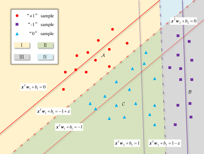
Figure 1: Two-dimensional illustration of one combination $(K_{i},K_{j})$ for twin multi-class support vector machine: The solid red line and the purple one represent two hyperplanes respectively; the red circle and the purple square represent two classes of samples, labeled as “$+1$” and “$-1$” respectively; the blue triangle belongs to the remaining classes, labeled as “0”. The region can be divided into four areas, i.e., Region I to IV respectively.

3.3 Model Transformation of the QPP (1)

Let $c_{1}=c_{2}=\frac{1}{\lambda_{1}}$, then the QPP (1) can be simplified as

$$\min\limits_{\bm{w}_{1},b_{1},\bm{\xi},\bm{\pi}}{} \frac{\lambda_{1}}{2}||\mathbf{A}\bm{w}_{1}+b_{1}\bm{e}_{n_{\mathrm{A}}}||^{2}+\bm{e}_{n_{\mathrm{B}}}^{\top}\bm{\xi}+\bm{e}_{n_{\mathrm{C}}}^{\top}\bm{\pi}$$ (3)

s.t. $$-(\mathbf{B}\bm{w}_{1}+b_{1}\bm{e}_{n_{\mathrm{B}}})+\bm{\xi}\geq\bm{e}_{n_{\mathrm{B}}},$$

$$-(\mathbf{C}\bm{w}_{1}+b_{1}\bm{e}_{n_{\mathrm{C}}})+\bm{\pi}\geq(1-\epsilon)\bm{e}_{n_{\mathrm{C}}},$$

$$\bm{\xi}\geq 0\bm{e}_{n_{\mathrm{B}}},~{}\bm{\pi}\geq 0\bm{e}_{n_{\mathrm{C}}}.$$

The Lagrangian function of the QPP (3) can be constructed as

$$\mathcal{L}_{1}= \frac{\lambda_{1}}{2}||\mathbf{A}\bm{w}_{1}+b_{1}\bm{e}_{n_{\mathrm{A}}}||^{2}+\bm{e}_{n_{\mathrm{B}}}^{\top}\bm{\xi}+\bm{e}_{n_{\mathrm{C}}}^{\top}\bm{\pi}$$ (4)

$$-{\bm{\alpha}^{\top}}[-(\mathbf{B}\bm{w}_{1}+b_{1}\bm{e}_{n_{\mathrm{B}}})+\bm{\xi}-\bm{e}_{n_{\mathrm{B}}}]$$

$$-{\bm{\beta}^{\top}}[-(\mathbf{C}\bm{w}_{1}+b_{1}\bm{e}_{n_{\mathrm{C}}})+\bm{\pi}-(1-\epsilon)\bm{e}_{n_{\mathrm{C}}}]$$

$$-{\bm{\gamma}^{\top}}\bm{\xi}-{\bm{\omega}^{\top}}\bm{\pi},$$

where $\bm{\alpha}\in\mathbb{R}^{n_{\mathrm{B}}}$, $\bm{\beta}\in\mathbb{R}^{n_{\mathrm{C}}}$, $\bm{\gamma}\in\mathbb{R}^{n_{\mathrm{B}}}$ and $\bm{\omega}\in\mathbb{R}^{n_{\mathrm{C}}}$ are the non-negative Lagrangian multipliers vectors. Set the partial derivatives of Equation 4 w.r.t. $\bm{w}_{1}$, $b_{1}$, $\bm{\xi}$ and $\bm{\pi}$ to 0, we can obtain

$$\frac{\partial\mathcal{L}_{1}}{\partial\bm{w}_{1}}= \lambda_{1}{\mathbf{A}^{\top}}(\mathbf{A}\bm{w}_{1}+b_{1}\bm{e}_{n_{\mathrm{A}}})+\mathbf{B}^{\top}\bm{\alpha}+\mathbf{C}^{\top}\bm{\beta}=0\bm{e}_{m},$$ (5)

$$\frac{\partial\mathcal{L}_{1}}{\partial b_{1}}= \lambda_{1}{\bm{e}_{n_{\mathrm{A}}}^{\top}}(\mathbf{A}\bm{w}_{1}+b_{1}\bm{e}_{n_{\mathrm{A}}})+\bm{e}_{n_{\mathrm{B}}}^{\top}\bm{\alpha}+\bm{e}_{n_{\mathrm{C}}}^{\top}\bm{\beta}=0,$$ (6)

$$\frac{\partial\mathcal{L}_{1}}{\partial\bm{\xi}}= \bm{e}_{n_{\mathrm{B}}}-\bm{\alpha}-\bm{\gamma}=0\bm{e}_{n_{\mathrm{B}}},$$ (7)

$$\frac{\partial\mathcal{L}_{1}}{\partial\bm{\pi}}= \bm{e}_{n_{\mathrm{C}}}-\bm{\beta}-\bm{\omega}=0\bm{e}_{n_{\mathrm{C}}}.$$ (8)

According to the Karush-Kuhn-Tucker (KKT) conditions, we have

$${\bm{\alpha}^{\top}}[-(\mathbf{B}\bm{w}_{1}+b_{1}\bm{e}_{n_{\mathrm{B}}})+\bm{\xi}-\bm{e}_{n_{\mathrm{B}}}]=0,$$ (9)

$${\bm{\beta}^{\top}}[-(\mathbf{C}\bm{w}_{1}+b_{1}\bm{e}_{n_{\mathrm{C}}})+\bm{\pi}-(1-\epsilon)\bm{e}_{n_{\mathrm{C}}}]=0,$$ (10)

$${\bm{\gamma}^{\top}}\bm{\xi}=0,$$ (11)

$${\bm{\omega}^{\top}}\bm{\pi}=0.$$ (12)

Combining Equations 5 and 6, we can obtain

$$\lambda_{1}\begin{bmatrix}\mathbf{A}^{\top}\\ \bm{e}_{n_{\mathrm{A}}}^{\top}\end{bmatrix}\begin{bmatrix}\mathbf{A}&\bm{e}_{n_{\mathrm{A}}}\end{bmatrix}\begin{bmatrix}\bm{w}_{1}\\ b_{1}\end{bmatrix}+\begin{bmatrix}\mathbf{B}^{\top}\\ \bm{e}_{n_{\mathrm{B}}}^{\top}\end{bmatrix}\bm{\alpha}+\begin{bmatrix}\mathbf{C}^{\top}\\ \bm{e}_{n_{\mathrm{C}}}^{\top}\end{bmatrix}\bm{\beta}=0\bm{e}_{m+1}.$$ (13)

Let $\mathbf{F}=[\mathbf{A},\bm{e}_{n_{\mathrm{A}}}]$, $\mathbf{G}=[\mathbf{B},\bm{e}_{n_{\mathrm{B}}}]$, $\mathbf{H}=[\mathbf{C},\bm{e}_{n_{\mathrm{C}}}]$ and $\bm{u}=[\bm{w}_{1};b_{1}]$. The above equation can be rewritten as

$$\lambda_{1}\mathbf{F}^{\top}\mathbf{F}\bm{u}+\mathbf{G}^{\top}\bm{\alpha}+\mathbf{H}^{\top}\bm{\beta}=0\bm{e}_{m+1}.$$ (14)

From Equation 13, the solution of the QPP (3) can be obtained when the matrix $\mathbf{F}^{\top}\mathbf{F}$ is invertible.

$$\bm{u}=-\frac{1}{\lambda_{1}}\mathbf{F}_{\mathrm{inv}}(\mathbf{G}^{\top}\bm{\alpha}+\mathbf{H}^{\top}\bm{\beta}),$$ (15)

where $\mathbf{F}_{\mathrm{inv}}$ represents the inverse matrix of $\mathbf{F}^{\top}\mathbf{F}$. Since the matrix $\mathbf{F}^{\top}\mathbf{F}$ is always semi-positive definite, we add the regularization term $\delta\mathbf{I}$ to avoid the ill-conditioning case in this work, where $\delta$ is a small positive real number and $\mathbf{I}$ is an identity matrix in $\mathbb{R}^{(m+1)\times(m+1)}$. Thus,

$$\mathbf{F}_{\mathrm{inv}}=(\mathbf{F}^{\top}\mathbf{F}+\delta\mathbf{I})^{-1}.$$ (16)

According to Equation 15, the function $f_{1}$ can be represented as

$$f_{1}(\bm{x})=-\frac{1}{\lambda_{1}}\begin{bmatrix}\bm{x}^{\top}&1\end{bmatrix}\mathbf{F}_{\mathrm{inv}}(\mathbf{G}^{\top}\bm{\alpha}+\mathbf{H}^{\top}\bm{\beta}).\\$$ (17)

3.4 Partition Strategies of the QPP (3)

From Equation 15, the Lagrangian multipliers $\bm{\alpha}$ and $\bm{\beta}$ of the QPP (3) correspond to the sample in $\mathcal{B}$ and $\mathcal{C}$, but not to that in $\mathcal{A}$. Hence, the samples in $\mathcal{B}$ and $\mathcal{C}$ need to be divided.

3.4.1 Partition Strategy of Samples in $\mathcal{B}$

Combining the non-negative properties of Lagrangian multipliers $\bm{\alpha},\bm{\gamma}$ with Equation 7, it is easy to obtain $0\bm{e}_{n_{\mathrm{B}}}\leq\bm{\alpha},\bm{\gamma}\leq\bm{e}_{n_{\mathrm{B}}}$. According to Hastie et al. (2004), by combining the constraint conditions in Equations 5, 6, 7 and 8 and the KKT conditions in Equations 9, 10, 11 and 12 of the QPP (3), we see that the sample $\bm{x}_{i}~{}(i\in\mathcal{B})$ can be discussed in three situations: when $-(\bm{x}_{i}^{\top}\bm{w}_{1}+b_{1})<1$, $\alpha_{i}=1$; when $-(\bm{x}_{i}^{\top}\bm{w}_{1}+b_{1})>1$, $\alpha_{i}=0$; when $-(\bm{x}_{i}^{\top}\bm{w}_{1}+b_{1})=1$, $\alpha_{i}$ can lie between 0 and 1.

Therefore, the samples in $\mathcal{B}$ can be divided into three sets, i.e., $\mathcal{L}_{\mathrm{B}}^{1}=\{i|-(\bm{x}_{i}^{\top}\bm{w}_{1}+b_{1})<1\}$, $\mathcal{E}_{\mathrm{B}}^{1}=\{i|-(\bm{x}_{i}^{\top}\bm{w}_{1}+b_{1})=1\}$, and $\mathcal{R}_{\mathrm{B}}^{1}=\{i|-(\bm{x}_{i}^{\top}\bm{w}_{1}+b_{1})>1\}$, as shown in Figure 2.

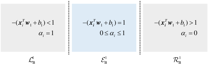
Figure 2: Partition of the sample set $\mathcal{B}$ for the QPP (3).

3.4.2 Partition Strategy for Samples in $\mathcal{C}$

Similar to Section 3.4.1, it is easy to see that the sample $\bm{x}_{k}~{}(k\in\mathcal{C})$ can be discussed in three situations: when $-(\bm{x}_{k}^{\top}\bm{w}_{1}+b_{1})<1-\epsilon$, $\beta_{k}=1$; when $-(\bm{x}_{k}^{\top}\bm{w}_{1}+b_{1})>1-\epsilon$, $\beta_{k}=0$; when $-(\bm{x}_{k}^{\top}\bm{w}_{1}+b_{1})=1-\epsilon$, $\beta_{k}$ can lie between 0 and 1.

Therefore, the samples in $\mathcal{C}$ can be divided into three sets, i.e., $\mathcal{L}_{\mathrm{C}}^{1}=\{k|-(\bm{x}_{k}^{\top}\bm{w}_{1}+b_{1})<1-\epsilon\}$, $\mathcal{E}_{\mathrm{C}}^{1}=\{k|-(\bm{x}_{k}^{\top}\bm{w}_{1}+b_{1})=1-\epsilon\}$, and $\mathcal{R}_{\mathrm{C}}^{1}=\{k|-(\bm{x}_{k}^{\top}\bm{w}_{1}+b_{1})>1-\epsilon\}$, as shown in Figure 3.

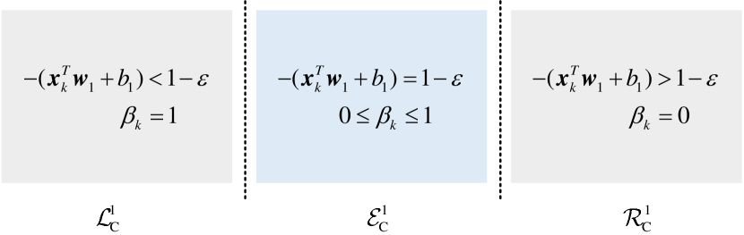
Figure 3: Partition of the sample set $\mathcal{C}$ for the QPP (3).

3.5 Model Transformation of the QPP (2)

Let $c_{3}=c_{4}=\frac{1}{\lambda_{2}}$, the QPP (2) can be rewritten as

$$\min\limits_{\bm{w}_{2},b_{2},\bm{\eta},\bm{\zeta}}{} \frac{\lambda_{2}}{2}||\mathbf{B}\bm{w}_{2}+b_{2}\bm{e}_{n_{\mathrm{B}}}||^{2}+\bm{e}_{n_{\mathrm{A}}}^{\top}\bm{\eta}+\bm{e}_{n_{\mathrm{C}}}^{\top}\bm{\zeta}$$ (18)

s.t. $$(\mathbf{A}\bm{w}_{2}+b_{2}\bm{e}_{n_{\mathrm{A}}})+\bm{\eta}\geq\bm{e}_{n_{\mathrm{A}}},$$

$$(\mathbf{C}\bm{w}_{2}+b_{2}\bm{e}_{n_{\mathrm{C}}})+\bm{\zeta}\geq(1-\epsilon)\bm{e}_{n_{\mathrm{C}}},$$

$$\bm{\eta}\geq 0\bm{e}_{n_{\mathrm{A}}},~{}\bm{\zeta}\geq 0\bm{e}_{n_{\mathrm{C}}}.$$

By constructing the Lagrangian function of Equation 18, we can obtain

$$\mathcal{L}_{2}= \frac{\lambda_{2}}{2}||\mathbf{B}\bm{w}_{2}+b_{2}\bm{e}_{n_{\mathrm{B}}}||^{2}+\bm{e}_{n_{\mathrm{A}}}^{\top}\bm{\eta}+\bm{e}_{n_{\mathrm{C}}}^{\top}\bm{\zeta}$$ (19)

$$-\bm{\mu}^{\top}[(\mathbf{A}\bm{w}_{2}+b_{2}\bm{e}_{n_{\mathrm{A}}})+\bm{\eta}-\bm{e}_{n_{\mathrm{A}}}]$$

$$-\bm{\rho}^{\top}[(\mathbf{C}\bm{w}_{2}+b_{2}\bm{e}_{n_{\mathrm{C}}})+\bm{\zeta}-(1-\epsilon)\bm{e}_{n_{\mathrm{C}}}]$$

$$-\bm{\phi}^{\top}\bm{\eta}-\bm{\psi}^{\top}\bm{\zeta},$$

where $\bm{\mu}\in\mathbb{R}^{n_{\mathrm{A}}}$, $\bm{\rho}\in\mathbb{R}^{n_{\mathrm{C}}}$, $\bm{\phi}\in\mathbb{R}^{n_{\mathrm{A}}}$ and $\bm{\psi}\in\mathbb{R}^{n_{\mathrm{C}}}$ are the non-negative Lagrangian multipliers vectors. Let the partial derivatives of Lagrangian function (19) w.r.t. $\bm{w}_{2}$, $b_{2}$, $\bm{\eta}$ and $\bm{\zeta}$ be 0 respectively, and we can get

$$\frac{\partial\mathcal{L}_{2}}{\partial\bm{w}_{1}}= \lambda_{2}{\mathbf{B}^{\top}}(\mathbf{B}\bm{w}_{2}+b_{2}\bm{e}_{n_{\mathrm{B}}})-\mathbf{A}^{\top}\bm{\mu}-\mathbf{C}^{\top}\bm{\rho}=0\bm{e}_{m},$$ (20)

$$\frac{\partial\mathcal{L}_{2}}{\partial b_{2}}= \lambda_{2}{\bm{e}_{n_{\mathrm{B}}}^{\top}}(\mathbf{B}\bm{w}_{2}+b_{2}\bm{e}_{n_{\mathrm{B}}})-\bm{e}_{n_{\mathrm{A}}}^{\top}\bm{\mu}-\bm{e}_{n_{\mathrm{C}}}^{\top}\bm{\rho}=0,$$ (21)

$$\frac{\partial\mathcal{L}_{2}}{\partial\bm{\eta}}= \bm{e}_{n_{\mathrm{A}}}-\bm{\mu}-\bm{\phi}=0\bm{e}_{n_{\mathrm{A}}},$$ (22)

$$\frac{\partial\mathcal{L}_{2}}{\partial\bm{\zeta}}= \bm{e}_{n_{\mathrm{C}}}-\bm{\rho}-\bm{\psi}=0\bm{e}_{n_{\mathrm{C}}}.$$ (23)

Combining the KKT conditions with the QPP (18), we can obtain

$$\bm{\mu}^{\top}[(\mathbf{A}\bm{w}_{2}+b_{2}\bm{e}_{n_{\mathrm{A}}})+\bm{\eta}-\bm{e}_{n_{\mathrm{A}}}]=0,$$ (24)

$$\bm{\rho}^{\top}[(\mathbf{C}\bm{w}_{2}+b_{2}\bm{e}_{n_{\mathrm{C}}})+\bm{\zeta}-(1-\epsilon)\bm{e}_{n_{\mathrm{C}}}]=0,$$ (25)

$$\bm{\phi}^{\top}\bm{\eta}=0,$$ (26)

$$\bm{\psi}^{\top}\bm{\zeta}=0.$$ (27)

From Equation 20 and Equation 21, we can obtain

$$\lambda_{2}\begin{bmatrix}\mathbf{B}^{\top}\\ \bm{e}_{n_{\mathrm{B}}}^{\top}\end{bmatrix}\begin{bmatrix}\mathbf{B}&\bm{e}_{n_{\mathrm{B}}}\end{bmatrix}\begin{bmatrix}\bm{w}_{2}\\ b_{2}\end{bmatrix}-\begin{bmatrix}\mathbf{A}^{\top}\\ \bm{e}_{n_{\mathrm{A}}}^{\top}\end{bmatrix}\bm{\mu}-\begin{bmatrix}\mathbf{C}^{\top}\\ \bm{e}_{n_{\mathrm{C}}}^{\top}\end{bmatrix}\bm{\rho}=0\bm{e}_{m+1}.$$ (28)

Let $\bm{v}=[\bm{w}_{2};b_{2}]$, the above equation can be rewritten as

$$\lambda_{2}\mathbf{G}^{\top}\mathbf{G}\bm{v}-\mathbf{F}^{\top}\bm{\mu}-\mathbf{H}^{\top}\bm{\rho}=0\bm{e}_{m+1}.$$ (29)

Therefore, the solution of the QPP (18) can be obtained when the matrix $\mathbf{G}^{\top}\mathbf{G}$ is invertible.

$$\bm{v}=\frac{1}{\lambda_{2}}\mathbf{G}_{\mathrm{inv}}(\mathbf{F}^{\top}\bm{\mu}+\mathbf{H}^{\top}\bm{\rho}),$$ (30)

where $\mathbf{G}_{\mathrm{inv}}$ represents the inverse matrix of $\mathbf{G}^{\top}\mathbf{G}$. Similar to Equation 16, we also add the regularization term $\delta\mathbf{I}$ to avoid the ill-conditioning case in this work.

$$\mathbf{G}_{\mathrm{inv}}=(\mathbf{G}^{\top}\mathbf{G}+\delta\mathbf{I})^{-1}.$$ (31)

According to Equation 30, the function $f_{2}$ can be represented as

$$f_{2}(\bm{x})=\frac{1}{\lambda_{2}}\begin{bmatrix}\bm{x}^{\top}&1\end{bmatrix}\mathbf{G}_{\mathrm{inv}}(\mathbf{F}^{\top}\bm{\mu}+\mathbf{H}^{\top}\bm{\rho}).\\$$ (32)

3.6 Partition Strategies of the QPP (18)

According to Equation 30, the Lagrangian multipliers $\bm{\mu}$ and $\bm{\rho}$ of the QPP (18) correspond to the sample in $\mathcal{A}$ and $\mathcal{C}$, but not to that in $\mathcal{B}$. Hence, the samples in $\mathcal{A}$ and $\mathcal{C}$ need to be divided.

3.6.1 Partition Strategy of Samples in $\mathcal{A}$

Combining the non-negative properties of Lagrangian multipliers $\bm{\mu},\bm{\phi}$ and Equation 22, it is easy to obtain $0\bm{e}_{n_{\mathrm{A}}}\leq\bm{\mu},\bm{\phi}\leq\bm{e}_{n_{\mathrm{A}}}$. According to Hastie et al. (2004), by combining the constraint conditions in Equations 20, 21, 22 and 23 and the KKT conditions in Equations 24, 25, 26 and 27 of the QPP (18), we see that the sample $\bm{x}_{i}~{}(i\in\mathcal{A})$ can be discussed in three situations: when $\bm{x}_{i}^{\top}\bm{w}_{2}+b_{2}<1$, $\mu_{i}=1$; when $\bm{x}_{i}^{\top}\bm{w}_{2}+b_{2}>1$, $\mu_{i}=0$; when $\bm{x}_{i}^{\top}\bm{w}_{2}+b_{2}=1$, $\mu_{i}$ can lie between 0 and 1.

Therefore, the samples in $\mathcal{A}$ can be divided into three sets, i.e., $\hbox{\pagecolor{myhlcolor}$\displaystyle\mathcal{L}_{\mathrm{A}}^{2}$}=\{i|-(\bm{x}_{i}^{\top}\bm{w}_{2}+b_{2})<1\}$, $\hbox{\pagecolor{myhlcolor}$\displaystyle\mathcal{E}_{\mathrm{A}}^{2}$}=\{i|-(\bm{x}_{i}^{\top}\bm{w}_{2}+b_{2})=1\}$, and $\hbox{\pagecolor{myhlcolor}$\displaystyle\mathcal{R}_{\mathrm{A}}^{2}$}=\{i|-(\bm{x}_{i}^{\top}\bm{w}_{2}+b_{2})>1\}$, as shown in Figure 4.

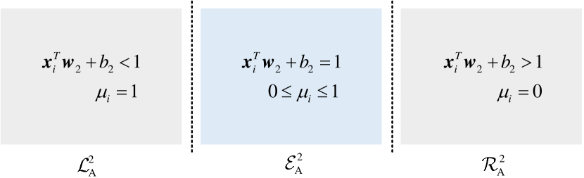
Figure 4: Partition of the sample set $\mathcal{A}$ for the QPP (18).

3.6.2 Partition Strategy for Samples in $\mathcal{C}$

Similar to Section 3.6.1, it is easy to see that the sample $\bm{x}_{k}~{}(k\in\mathcal{C})$ can be discussed in three situations: when $\bm{x}_{k}^{\top}\bm{w}_{2}+b_{2}<1-\epsilon$, $\rho_{k}=1$; when $\bm{x}_{k}^{\top}\bm{w}_{2}+b_{2}>1-\epsilon$, $\rho_{k}=0$; when $\bm{x}_{k}^{\top}\bm{w}_{2}+b_{2}=1-\epsilon$, $\rho_{k}$ can lie between 0 and 1.

Therefore, the samples in $\mathcal{C}$ can be divided into three sets, i.e., $\hbox{\pagecolor{myhlcolor}$\displaystyle\mathcal{L}_{\mathrm{C}}^{2}$}=\{k|-(\bm{x}_{k}^{\top}\bm{w}_{2}+b_{2})<1-\epsilon\}$, $\hbox{\pagecolor{myhlcolor}$\displaystyle\mathcal{E}_{\mathrm{C}}^{2}$}=\{k|-(\bm{x}_{k}^{\top}\bm{w}_{2}+b_{2})=1-\epsilon\}$, and $\hbox{\pagecolor{myhlcolor}$\displaystyle\mathcal{R}_{\mathrm{C}}^{2}$}=\{k|-(\bm{x}_{k}^{\top}\bm{w}_{2}+b_{2})>1-\epsilon\}$, as shown in Figure 5.

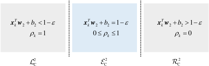
Figure 5: Partition of the sample set $\mathcal{C}$ for the QPP (18).

4 Solution Path for Twin Multi-class Support Vector Machine

This section aims to find the entire regularized solutions for all the values of the regularization parameter $\lambda>0$. To this end, we first prove that the solution is piecewise linear w.r.t. $\lambda$, which greatly reduces computational cost. Let $\lambda$ go from very large to 0, and then we just need to find all the break points for the $\lambda$ to figure out the entire solution path.

4.1 Piecewise Linear Theory

The matrices $\mathbf{F}_{\mathrm{E}}$, $\mathbf{G}_{\mathrm{E}}$ and $\mathbf{H}_{\mathrm{E}}$ are used to represent the sample matrix composed of the elbow $\mathcal{E}_{\mathrm{A}}$, $\mathcal{E}_{B}$ and $\mathcal{E}_{C}$. Let $n_{\mathrm{A}}=|\mathcal{E}_{\mathrm{A}}|$, $n_{\mathrm{B}}=|\mathcal{E}_{B}|$, $n_{\mathrm{C}}=|\mathcal{E}_{C}|$, $n_{\mathrm{BC}}=|\mathcal{E}_{B}|+|\mathcal{E}_{C}|$ and $n_{\mathrm{AC}}=|\mathcal{E}_{\mathrm{A}}|+|\mathcal{E}_{C}|$. For convenient notations, the $l$-th step parameters are assigned a superscript ‘$l$’ and that of the two QPPs are assigned a superscript ‘$1$’ and ‘$2$’, respectively. For example, $\mathcal{E}_{\mathrm{B}}^{1,l}$ denotes the $l$-step index set w.r.t. the first QPP.

4.1.1 Piecewise Linear w.r.t. $\lambda_{1}$

Theorem 1 can be used to prove that the Lagrangian multipliers $\bm{\alpha}$ and $\bm{\beta}$ are piecewise linear w.r.t. the regularization parameter $\lambda_{1}$.

Theorem 1.

For the QPP (3), $\lambda_{1}^{l}>\lambda_{1}>\lambda_{1}^{l+1}$, if the matrix

$$\mathbf{E}_{\mathrm{BC}}^{l}=\begin{bmatrix}\mathbf{G}_{\mathrm{E}}^{l}\\ \mathbf{H}_{\mathrm{E}}^{l}\end{bmatrix}\mathbf{F}_{\mathrm{inv}}\begin{bmatrix}(\mathbf{G}_{\mathrm{E}}^{l})^{\top}&(\mathbf{H}_{\mathrm{E}}^{l})^{\top}\end{bmatrix}$$ (33)

is invertible, then the Lagrangian multipliers $\alpha_{i}~{}(i=1,2,\cdots,n_{\mathrm{B}}^{l})$ and $\beta_{k}~{}(k=1,2,\cdots,n_{\mathrm{C}}^{l})$ are piecewise linear w.r.t. the regularization parameter $\lambda_{1}$ respectively, which can be mathematically described below:

$$\alpha_{i} =\alpha_{i}^{l}-(\lambda^{l}-\lambda)\theta_{i}^{l},$$ (34)

$$\beta_{k} =\beta_{k}^{l}-(\lambda^{l}-\lambda)\theta_{n_{\mathrm{B}}^{l}+k}^{l},$$ (35)

where

$$\bm{\theta}^{l} =(\mathbf{E}_{\mathrm{BC}}^{l})^{-1}\begin{bmatrix}\bm{e}_{n_{\mathrm{B}}^{l}}\\ (1-\epsilon)\bm{e}_{n_{\mathrm{C}}^{l}}\end{bmatrix}$$ (36)

$$=(\mathbf{E}_{\mathrm{BC}}^{l})^{-1}\hbox{\pagecolor{myhlcolor}$\displaystyle\bm{e}_{n_{\mathrm{BC}}}^{l}$}.$$

Proof.

Theorem 1 can be proved in two steps, i.e., proving that Lagrangian multipliers $\alpha_{i}~{}(i=1,2,\cdots,n_{\mathrm{B}}^{l})$ and $\beta_{k}~{}(k=1,2,\cdots,n_{\mathrm{C}}^{l})$ are piecewise linear w.r.t. the regularization parameter $\lambda_{1}$ respectively.

First of all, the $l$-th step function of Equation 17 is

$$f_{1}^{l}(\bm{x})=-\frac{1}{\lambda_{1}^{l}}\begin{bmatrix}\bm{x}^{\top}&1\end{bmatrix}\mathbf{F}_{\mathrm{inv}}(\mathbf{G}^{\top}\bm{\alpha}^{l}+\mathbf{H}^{\top}\bm{\beta}^{l}).\\$$ (37)

By the following transformation about $f_{1}$ and $f_{1}^{l}$, we can obtain

$$f_{1}(\bm{x})= \frac{\lambda_{1}^{l}}{\lambda_{1}}f_{1}^{l}(\bm{x})+f_{1}(\bm{x})-\frac{\lambda_{1}^{l}}{\lambda_{1}}f_{1}^{l}(\bm{x})$$ (38)

$$= \frac{1}{\lambda_{1}}\{\lambda_{1}^{l}f_{1}^{l}(\bm{x})+\begin{bmatrix}\bm{x}^{\top}&1\end{bmatrix}\mathbf{F}_{\mathrm{inv}}[\mathbf{G}^{\top}(\bm{\alpha}^{l}-\bm{\alpha})+\mathbf{H}^{\top}(\bm{\beta}^{l}-\bm{\beta})]\}.$$

For $\forall i\in\mathcal{L}_{\mathrm{B}}^{1,l}\cup\mathcal{R}_{\mathrm{B}}^{1,l}$ and $\forall k\in\mathcal{L}_{\mathrm{C}}^{1,l}\cup\mathcal{R}_{\mathrm{C}}^{1,l}$, there are $\alpha_{i}^{l}-\alpha_{i}=0$ and $\beta_{k}^{l}-\beta_{k}=0$ respectively. Therefore, the above equation (38) can be simplified as

$$f_{1}(\bm{x})= \frac{1}{\lambda_{1}}\{\lambda_{1}^{l}f_{1}^{l}(\bm{x})+\begin{bmatrix}\bm{x}^{\top}&1\end{bmatrix}\mathbf{F}_{\mathrm{inv}}[\mathbf{G}_{\mathrm{E}}^{\top}(\bm{\alpha}_{\mathrm{E}}^{l}-\bm{\alpha}_{\mathrm{E}})+\mathbf{H}^{\top}(\bm{\beta}^{l}_{\mathrm{E}}-\bm{\beta}_{\mathrm{E}})]\}$$ (39)

$$= \frac{1}{\lambda_{1}}\{\lambda_{1}^{l}f_{1}^{l}(\bm{x})+\begin{bmatrix}\bm{x}^{\top}&1\end{bmatrix}\mathbf{F}_{\mathrm{inv}}\begin{bmatrix}(\mathbf{G}_{\mathrm{E}}^{l})^{\top}&(\mathbf{H}_{\mathrm{E}}^{l})^{\top}\end{bmatrix}\begin{bmatrix}\bm{\alpha}_{\mathrm{E}}^{l}-\bm{\alpha}_{\mathrm{E}}\\ \bm{\beta}_{\mathrm{E}}^{l}-\bm{\beta}_{\mathrm{E}}\end{bmatrix}\}.$$

For $\forall i\in\mathcal{E}_{\mathrm{B}}^{1,l}$ and $\forall k\in\mathcal{E}_{\mathrm{C}}^{1,l}$, there are $-f_{1}(\bm{x}_{i})=-f_{1}^{l}(\bm{x}_{i})=1$ and $-f_{1}(\bm{x}_{k})=-f_{1}^{l}(\bm{x}_{k})=1-\epsilon$ respectively. Substitute these two obtained conditions to Equation 39 and combine it with Equation 33, the following system of linear equation w.r.t. the Lagrangian multipliers $\mathbf{\alpha}_{\mathrm{E}}$ and $\mathbf{\beta}_{\mathrm{E}}$ can be deduced.

$$\begin{bmatrix}\mathbf{G}_{\mathrm{E}}^{l}\\ \mathbf{H}_{\mathrm{E}}^{l}\end{bmatrix}\mathbf{F}_{\mathrm{inv}}\begin{bmatrix}(\mathbf{G}_{\mathrm{E}}^{l})^{\top}&(\mathbf{H}_{\mathrm{E}}^{l})^{\top}\end{bmatrix}\begin{bmatrix}\bm{\alpha}_{\mathrm{E}}^{l}-\bm{\alpha}_{\mathrm{E}}\\ \bm{\beta}_{\mathrm{E}}^{l}-\bm{\beta}_{\mathrm{E}}\end{bmatrix} =\mathbf{E}_{\mathrm{BC}}^{l}\begin{bmatrix}\bm{\alpha}_{\mathrm{E}}^{l}-\bm{\alpha}_{\mathrm{E}}\\ \bm{\beta}_{\mathrm{E}}^{l}-\bm{\beta}_{\mathrm{E}}\end{bmatrix}$$ (40)

$$=(\lambda_{1}^{l}-\lambda_{1})\hbox{\pagecolor{myhlcolor}$\displaystyle\bm{e}_{n_{\mathrm{BC}}}^{l}$}.$$

If the matrix $\mathbf{E}_{\mathrm{BC}}^{l}$ is invertible, then we can obtain

$$\begin{bmatrix}\bm{\alpha}_{\mathrm{E}}^{l}-\bm{\alpha}_{\mathrm{E}}\\ \bm{\beta}_{\mathrm{E}}^{l}-\bm{\beta}_{\mathrm{E}}\end{bmatrix} =(\lambda_{1}^{l}-\lambda_{1})(\mathbf{E}_{\mathrm{BC}}^{l})^{-1}\hbox{\pagecolor{myhlcolor}$\displaystyle\bm{e}_{n_{\mathrm{BC}}}^{l}$}$$ (41)

$$=(\lambda_{1}^{l}-\lambda_{1})\bm{\theta}^{l}.$$

In conclusion, Theorem 1 is proved. ∎

According to Theorem 1, it is easy to obtain the following corollary:

Corollary 1.

For the QPP (3), $\lambda_{1}^{l}>\lambda_{1}>\lambda_{1}^{l+1}$, the function $f_{1}$ is piecewise linear w.r.t. $\frac{1}{\lambda_{1}}$, i.e.,

$$f_{1}(\bm{x}) =\frac{1}{\lambda_{1}}[\lambda_{1}^{l}f_{1}^{l}(\bm{x})+(\lambda_{1}^{l}-\lambda_{1})g^{l}(\bm{x})]$$ (42)

$$=\frac{\lambda_{1}^{l}}{\lambda_{1}}[f_{1}^{l}(\bm{x}+g^{l}(\bm{x})]-g^{l}(\bm{x}),$$

where

$$g^{l}(\bm{x})=\begin{bmatrix}\bm{x}^{\top}&1\end{bmatrix}\mathbf{F}_{\mathrm{inv}}\begin{bmatrix}(\mathbf{G}_{\mathrm{E}}^{l})^{\top}&(\mathbf{H}_{\mathrm{E}}^{l})^{\top}\end{bmatrix}\bm{\theta}^{l}.$$ (43)

4.1.2 Piecewise Linear w.r.t. $\lambda_{2}$

Analogously, Theorem 2 can be used to prove that the Lagrangian multipliers $\bm{\mu}$ and $\bm{\rho}$ are piecewise linear w.r.t. the regularization parameter $\lambda_{2}$.

Theorem 2.

For the QPP (18), $\lambda_{2}^{l}>\lambda_{2}>\lambda_{2}^{l+1}$, if the matrix

$$\mathbf{E}_{\mathrm{AC}}^{l}=\begin{bmatrix}\mathbf{F}_{\mathrm{E}}^{l}\\ \mathbf{H}_{\mathrm{E}}^{l}\end{bmatrix}\mathbf{G}_{\mathrm{inv}}\begin{bmatrix}(\mathbf{F}_{\mathrm{E}}^{l})^{\top}&(\mathbf{H}_{\mathrm{E}}^{l})^{\top}\end{bmatrix}$$ (44)

is invertible, then the Lagrangian multipliers $\mu_{i}~{}(i=1,2,\cdots,n_{\mathrm{A}}^{l})$ and $\rho_{k}~{}(k=1,2,\cdots,n_{\mathrm{C}}^{l})$ are piecewise linear w.r.t. the regularization parameter $\lambda_{2}$ respectively, which can be mathematically described below:

$$\mu_{i} =\mu_{i}^{l}-(\lambda^{l}-\lambda)\vartheta_{i}^{l},$$ (45)

$$\rho_{k} =\rho_{k}^{l}-(\lambda^{l}-\lambda)\vartheta_{n_{\mathrm{A}}^{l}+k}^{l},$$ (46)

where

$$\bm{\vartheta}^{l} =(\mathbf{E}_{\mathrm{AC}}^{l})^{-1}\begin{bmatrix}\bm{e}_{n_{\mathrm{A}}^{l}}\\ (1-\epsilon)\bm{e}_{n_{\mathrm{C}}^{l}}\end{bmatrix}$$ (47)

$$=(\mathbf{E}_{\mathrm{AC}}^{l})^{-1}\hbox{\pagecolor{myhlcolor}$\displaystyle\bm{e}_{n_{\mathrm{AC}}}^{l}$}.$$

Proof.

Theorem 2 can be proved in two steps, i.e., proving that Lagrangian multipliers $\mu_{i}~{}(i=1,2,\cdots,n_{\mathrm{A}}^{l})$ and $\rho_{k}~{}(k=1,2,\cdots,n_{\mathrm{C}}^{l})$ are piecewise linear w.r.t. the regularization parameter $\lambda_{2}$ respectively.

First of all, the $l$-th step function of Equation 32 is

$$f_{2}^{l}(\bm{x})=\frac{1}{\lambda_{2}^{l}}\begin{bmatrix}\bm{x}^{\top}&1\end{bmatrix}\mathbf{G}_{\mathrm{inv}}(\mathbf{F}^{\top}\bm{\mu}^{l}+\mathbf{H}^{\top}\bm{\rho}^{l}).\\$$ (48)

By the following transformation about $f_{2}$ and $f_{2}^{l}$, we can obtain

$$f_{2}(\bm{x})= \frac{\lambda_{2}^{l}}{\lambda_{2}}f_{2}^{l}(\bm{x})+f_{2}(\bm{x})-\frac{\lambda_{2}^{l}}{\lambda_{2}}f_{2}^{l}(\bm{x})$$ (49)

$$= \frac{1}{\lambda_{2}}\{\lambda_{2}^{l}f_{2}^{l}(\bm{x})-\begin{bmatrix}\bm{x}^{\top}&1\end{bmatrix}\mathbf{G}_{\mathrm{inv}}[\mathbf{F}^{\top}(\bm{\mu}^{l}-\bm{\mu})+\mathbf{H}^{\top}(\bm{\rho}^{l}-\bm{\rho})]\}.$$

For $\forall i\in\mathcal{L}_{\mathrm{A}}^{1,l}\cup\mathcal{R}_{\mathrm{A}}^{1,l}$ and $\forall k\in\mathcal{L}_{\mathrm{C}}^{1,l}\cup\mathcal{R}_{\mathrm{C}}^{1,l}$, there are $\mu_{i}^{l}-\mu_{i}=0$ and $\rho_{k}^{l}-\rho_{k}=0$ respectively. Therefore, the above equation (49) can be simplified as

$$f_{2}(\bm{x})= \frac{1}{\lambda_{2}}\{\lambda_{2}^{l}f_{2}^{l}(\bm{x})-\begin{bmatrix}\bm{x}^{\top}&1\end{bmatrix}\mathbf{G}_{\mathrm{inv}}[\mathbf{F}_{\mathrm{E}}^{\top}(\bm{\mu}_{\mathrm{E}}^{l}-\bm{\mu}_{\mathrm{E}})+\mathbf{H}^{\top}(\bm{\rho}^{l}_{\mathrm{E}}-\bm{\rho}_{\mathrm{E}})]\}$$ (50)

$$= \frac{1}{\lambda_{2}}\{\lambda_{2}^{l}f_{2}^{l}(\bm{x})-\begin{bmatrix}\bm{x}^{\top}&1\end{bmatrix}\mathbf{G}_{\mathrm{inv}}\begin{bmatrix}(\mathbf{F}_{\mathrm{E}}^{l})^{\top}&(\mathbf{H}_{\mathrm{E}}^{l})^{\top}\end{bmatrix}\begin{bmatrix}\bm{\mu}_{\mathrm{E}}^{l}-\bm{\mu}_{\mathrm{E}}\\ \bm{\rho}_{\mathrm{E}}^{l}-\bm{\rho}_{\mathrm{E}}\end{bmatrix}\}.$$

For $\forall i\in\mathcal{E}_{\mathrm{A}}^{1,l}$ and $\forall k\in\mathcal{E}_{\mathrm{C}}^{1,l}$, there are $f_{2}(\bm{x}_{i})=f_{2}^{l}(\bm{x}_{i})=1$ and $f_{2}(\bm{x}_{k})=f_{2}^{l}(\bm{x}_{k})=1-\epsilon$ respectively. Substitute theses two obtained conditions to Equation 50 and combine it with Equation 44, the following system of linear equation w.r.t. the Lagrangian multipliers $\mathbf{\mu}_{\mathrm{E}}$ and $\mathbf{\rho}_{\mathrm{E}}$ can be deduced.

$$\begin{bmatrix}\mathbf{F}_{\mathrm{E}}^{l}\\ \mathbf{H}_{\mathrm{E}}^{l}\end{bmatrix}\mathbf{G}_{\mathrm{inv}}\begin{bmatrix}(\mathbf{F}_{\mathrm{E}}^{l})^{\top}&(\mathbf{H}_{\mathrm{E}}^{l})^{\top}\end{bmatrix}\begin{bmatrix}\bm{\mu}_{\mathrm{E}}^{l}-\bm{\mu}_{\mathrm{E}}\\ \bm{\rho}_{\mathrm{E}}^{l}-\bm{\rho}_{\mathrm{E}}\end{bmatrix} =\mathbf{E}_{\mathrm{AC}}^{l}\begin{bmatrix}\bm{\mu}_{\mathrm{E}}^{l}-\bm{\mu}_{\mathrm{E}}\\ \bm{\rho}_{\mathrm{E}}^{l}-\bm{\rho}_{\mathrm{E}}\end{bmatrix}$$ (51)

$$=(\lambda_{2}^{l}-\lambda_{2})\hbox{\pagecolor{myhlcolor}$\displaystyle\bm{e}_{n_{\mathrm{AC}}}^{l}$}.$$

If the matrix $\mathbf{E}_{\mathrm{AC}}^{l}$ is invertible, then we can obtain

$$\begin{bmatrix}\bm{\mu}_{\mathrm{E}}^{l}-\bm{\mu}_{\mathrm{E}}\\ \bm{\rho}_{\mathrm{E}}^{l}-\bm{\rho}_{\mathrm{E}}\end{bmatrix} =(\lambda_{2}^{l}-\lambda_{2})(\mathbf{E}_{\mathrm{AC}}^{l})^{-1}\hbox{\pagecolor{myhlcolor}$\displaystyle\bm{e}_{n_{\mathrm{AC}}}^{l}$}$$ (52)

$$=(\lambda_{2}^{l}-\lambda_{2})\bm{\vartheta}^{l}.$$

In conclusion, Theorem 2 is proved. ∎

According to Theorem 2, it can be obtained the following corollary:

Corollary 2.

For the QPP (18), $\lambda_{2}^{l}>\lambda_{2}>\lambda_{2}^{l+1}$, the function $f_{2}$ is piecewise linear w.r.t. $\frac{1}{\lambda_{2}}$.

$$f_{2}(\bm{x}) =\frac{1}{\lambda_{2}}[\lambda_{2}^{l}f_{2}^{l}(\bm{x})-(\lambda_{2}^{l}-\lambda_{2})h^{l}(\bm{x})]$$ (53)

$$=\frac{\lambda_{2}^{l}}{\lambda_{2}}[f_{2}^{l}(\bm{x})-h^{l}(\bm{x})]+h^{l}(\bm{x}),$$

where

$$h^{l}(\bm{x})=\begin{bmatrix}\bm{x}^{\top}&1\end{bmatrix}\mathbf{G}_{\mathrm{inv}}\begin{bmatrix}(\mathbf{F}_{\mathrm{E}}^{l})^{\top}&(\mathbf{H}_{\mathrm{E}}^{l})^{\top}\end{bmatrix}\bm{\vartheta}^{l}.$$ (54)

4.2 Initialization

When the regularization parameters are infinite, it is easy to prove that the corresponding Lagrangian multipliers are 1. Based on this result, we design an initialization algorithm to get the starting conditions.

4.2.1 Initializing $\lambda_{1}^{0}$

The general idea of initialization is to find the value of the Lagrangian multipliers $\bm{\alpha}$ and $\beta$ as the regularization parameter $\lambda_{1}^{0}$ approaches infinity, which can be concluded in Theorem 3.

Theorem 3.

For the QPP (3), when the regularization parameter $\lambda_{1}^{0}$ is close to infinity, the Lagrangian multipliers $\alpha_{i}^{0}~{}(i=1,2,\cdots,n_{\mathrm{B}}^{0})$ and $\beta_{k}^{0}~{}(k=1,2,\cdots,n_{\mathrm{C}}^{0})$ are equal to 1, i.e., $\lambda_{1}^{0}\rightarrow+\infty\Rightarrow\alpha_{i}^{0}=\beta_{k}^{0}=1$,

Proof.

When $\lambda_{1}^{0}\rightarrow+\infty$, we can obtain $-f_{1}(\bm{x}_{i})=0<1-\epsilon<1$ from Equation 17. From Figure 2, $-f_{1}(\bm{x}_{i})<1$ is equivalent to $\alpha_{i}=1$. From Figure 3, $-f_{1}(\bm{x}_{k})<1-\epsilon$ is equivalent to $\beta_{k}=1$.

In conclusion, Theorem 3 is proved. ∎

4.2.2 Initializing $\lambda_{2}^{0}$

Accordingly, Theorem 4 is used to find the value of the Lagrangian multipliers $\bm{\mu}$ and $\bm{\rho}$ as the regularization parameter $\lambda_{2}^{0}$ approaches the infinity.

Theorem 4.

For the QPP (18), when the regularization parameter $\lambda_{2}^{0}$ is close to infinity, the Lagrangian multipliers $\mu_{i}^{0}~{}(i=1,2,\cdots,n_{\mathrm{A}}^{0})$ and $\rho_{k}~{}(k=1,2,\cdots,n_{\mathrm{C}}^{0})$ are equal to 1, i.e., $\lambda_{2}^{0}\rightarrow+\infty\Rightarrow\mu_{i}^{0}=\rho_{k}^{0}=1$,

Proof.

When $\lambda_{2}^{0}\rightarrow+\infty$, we can obtain $f_{1}(\bm{x}_{i})=0<1-\epsilon<1$ according to Equation 17. From Figure 4, $f_{1}(\bm{x}_{i})<1$ is equivalent to $\mu_{i}=1$. From Figure 5, $f_{1}(\bm{x}_{k})<1-\epsilon$ is equivalent to $\rho_{k}=1$.

In conclusion, Theorem 4 is proved. ∎

4.2.3 Initialization Algorithm

According to Theorems 3 and 4, it is obvious that Lagrangian multipliers are equal to 1 as the regularization parameter approaches infinity. At this point, the samples are all on the left of the elbow. The basic idea of initialization is to gradually reduce the regularization parameter until the first sample point reaches the elbow. Algorithm 1 describes the detailed process of initialization for the QPP (3), and it is in the same way for the QPP (18).

Input: System parameters $\delta$, $\epsilon$ and sample matrices $\mathbf{A}$, $\mathbf{B}$ and $\mathbf{C}$.

Output: Initial parameters $\lambda_{1}^{0}$, initial Lagrangian multipliers $\alpha_{i}^{0}$, $\beta_{k}^{0}$, and initial index sets $\mathcal{L}_{\mathrm{B}}^{1,0}$, $\mathcal{E}_{\mathrm{B}}^{1,0}$, $\mathcal{R}_{\mathrm{B}}^{1,0}$, $\mathcal{L}_{\mathrm{C}}^{1,0}$, $\mathcal{E}_{\mathrm{C}}^{1,0}$ and $\mathcal{R}_{\mathrm{C}}^{1,0}$.

// Variable preparation phase

$\bm{\alpha}^{0}\leftarrow\bm{e}_{n_{\mathrm{B}}}$, $n_{\mathrm{B}}\leftarrow\mathrm{size}(\mathbf{B},1)$;

  // By Theorem 3.

$\bm{\beta}^{0}\leftarrow\bm{e}_{n_{\mathrm{C}}}$, $n_{\mathrm{B}}\leftarrow\mathrm{size}(\mathbf{C},1)$;

  // By Theorem 3.

1 Obtain homogeneous matrices $\mathbf{F}$, $\mathbf{G}$ and $\mathbf{H}$ from $\mathbf{A}$, $\mathbf{B}$ and $\mathbf{C}$;

2 $\mathbf{I}\leftarrow\mathrm{eye}(m+1)$, $m\leftarrow\mathrm{size}(\mathbf{A},1)$;

$\mathbf{F}_{\mathrm{inv}}\leftarrow(\mathbf{F}^{\top}\mathbf{F}+\delta\mathbf{I})^{-1}$ ;

  // By Equation 16

$\lambda_{1}^{0}\leftarrow 0$;

  // Initialize a minimum number to $\lambda_{1}^{0}$

3 $\mathcal{R}_{\mathrm{B}}^{1,0}$, $\mathcal{R}_{\mathrm{C}}^{1,0}\leftarrow\varnothing,\varnothing$;

// Initialization phase for samples in $\mathcal{B}$: see Section 4.2.1

4 foreach $i\in\mathcal{B}$ do

       $\lambda=\begin{bmatrix}\bm{x}_{i}^{\top}&1\end{bmatrix}\mathbf{F}_{\mathrm{inv}}(\mathbf{G}^{\top}\bm{\alpha}^{0}+\mathbf{H}^{\top}\bm{\beta}^{0})$;

        // By Equation 17

5       if $\lambda>\lambda_{1}^{0}$ then

             $\lambda_{1}^{0}\leftarrow\lambda$;

              // Update the regularization parameter by

             $\mathcal{L}_{\mathrm{B}}^{1,0},\mathcal{E}_{\mathrm{B}}^{1,0}\leftarrow\{{1,\cdots,i-1,i+1,\cdots,n_{\mathrm{B}}}\},\{i\}$ ;

              // Initialize samples in $\mathcal{B}$ when $\mathcal{L}_{\mathrm{B}}\rightarrow\mathcal{E}_{\mathrm{B}}$

             $\mathcal{L}_{\mathrm{C}}^{1,0},\mathcal{E}_{\mathrm{C}}^{1,0}\leftarrow\{{1,2,\cdots,n_{\mathrm{B}}}\},\varnothing$ ;

              // Initialize samples in $\mathcal{C}$

6            

7       end if

8      

9 end foreach

// Initialization phase for samples in $\mathcal{C}$: see Section 4.2.2

10 foreach $k\in\mathcal{C}$ do

       $\lambda=\frac{1}{1-\epsilon}\begin{bmatrix}\bm{x}_{k}^{\top}&1\end{bmatrix}\mathbf{F}_{\mathrm{inv}}(\mathbf{G}^{\top}\bm{\alpha}^{0}+\mathbf{H}^{\top}\bm{\beta}^{0})$;

        // By Equation 17

11       if $\lambda>\lambda_{1}^{0}$ then

             $\lambda_{1}^{0}\leftarrow\lambda$;

              // Update the regularization parameter by

             $\mathcal{L}_{\mathrm{C}}^{1,0},\mathcal{E}_{\mathrm{C}}^{1,0}\leftarrow\{{1,\cdots,i-1,i+1,\cdots,n_{\mathrm{C}}}\},\{i\}$ ;

              // Initialize samples in $\mathcal{C}$ when $\mathcal{L}_{\mathrm{C}}\rightarrow\mathcal{E}_{\mathrm{C}}$

             $\mathcal{L}_{\mathrm{B}}^{1,0},\mathcal{E}_{\mathrm{B}}^{1,0}\leftarrow\{{1,2,\cdots,n_{\mathrm{B}}}\},\varnothing$ ;

              // Initialize samples in $\mathcal{B}$

12            

13       end if

14      

15 end foreach

16return $\lambda_{1}^{0}$, $\alpha_{i}^{0}$, $\beta_{k}^{0}$, $\mathcal{L}_{\mathrm{B}}^{1,0}$, $\mathcal{E}_{\mathrm{B}}^{1,0}$, $\mathcal{R}_{\mathrm{B}}^{1,0}$, $\mathcal{L}_{\mathrm{C}}^{1,0}$, $\mathcal{E}_{\mathrm{C}}^{1,0}$ and $\mathcal{R}_{\mathrm{C}}^{1,0}$;

Algorithm 1 Initialization Algorithm of the QPP (3)

4.3 Finding $\lambda^{l+1}$

The aim of finding $\lambda^{l+1}$ is to update the regularization parameter as long as the corresponding parameters, such as sample sets and Lagrangian multipliers. Before designing the updating strategy, we first give the definition of the event and starting event, as follows:

Definition 1.

As the regularization parameter changes, the sample index set will also be updated, and this change is defined as an event in this work, represented by a symbolic "$\rightarrow$".

Definition 2.

If more than one event can occur, the event with the largest regularization parameter value is selected to occur first and is defined as the starting event in this work.

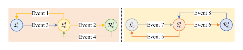
Figure 6: Possible events for the QPP (3): there are two scenarios and eight events for the sample sets $\mathcal{B}$ (left) and $\mathcal{C}$ (right).

As analyzed in Section 3.4, the changes of samples in sets $\mathcal{B}$ and $\mathcal{C}$ need to be discussed for the QPP (3). From Definition 1, there are eight kinds of possible events in total, illustrated in Figure 6. Next, we elaborate on them one by one.

If $\mathcal{E}_{\mathrm{B}}^{1}\neq\varnothing$, then one of the sample points in $\mathcal{E}_{\mathrm{B}}^{1}$ may go into either $\mathcal{L}_{\mathrm{B}}^{1}$ or $\mathcal{R}_{\mathrm{B}}^{1}$.

1. If $\mathcal{E}_{\mathrm{B}}^{1}\rightarrow\mathcal{L}_{\mathrm{B}}^{1}$, then $\alpha_{i}$ changes from $0\leq\alpha_{i}\leq 1$ to $\alpha_{i}=1$ and $f_{1}(\bm{x}_{i})$ changes from $-f_{1}(\bm{x}_{i})=1$ to $-f_{1}(\bm{x}_{i})<1$. Combining $\alpha_{i}=1$ with Equation 34, we can obtain the corresponding regularization parameter $\lambda_{1}^{1}$ by

   $$\lambda_{1}^{1}=\max_{i\in\mathcal{E}^{1,l}_{\mathrm{B}}}\{\lambda_{1}^{l}-\frac{\alpha^{l}_{i}-\alpha_{i}}{\theta^{l}_{i}}\}=\max_{i\in\mathcal{E}^{1,l}_{\mathrm{B}}}\{\lambda_{1}^{l}-\frac{\alpha^{l}_{i}-1}{\theta^{l}_{i}}\},$$ (55)

   where $\theta^{l}_{i}<0$.

1. If $\mathcal{E}_{\mathrm{B}}^{1}\rightarrow\mathcal{R}_{\mathrm{B}}^{1}$, then $\alpha_{i}$ changes from $0\leq\alpha_{i}\leq 1$ to $\alpha_{i}=0$ and $f_{1}(\bm{x}_{i})$ changes from $-f_{1}(\bm{x}_{i})=1$ to $-f_{1}(\bm{x}_{i})>1$. Combining $\alpha_{i}=0$ with Equation 34, we can obtain the corresponding regularization parameter $\lambda_{1}^{2}$ by

   $$\lambda_{1}^{2}=\max_{i\in\mathcal{E}^{1,l}_{\mathrm{B}}}\{\lambda_{1}^{l}-\frac{\alpha^{l}_{i}-\alpha_{i}}{\hbox{\pagecolor{myhlcolor}$\displaystyle\theta^{l}_{i}$}}\}=\max_{i\in\mathcal{E}^{1,l}_{\mathrm{B}}}\{\lambda_{1}^{l}-\frac{\alpha^{l}_{i}}{\theta^{l}_{i}}\},$$ (56)

   where $\theta^{l}_{i}>0$.

If $\mathcal{L}_{\mathrm{B}}^{1}\neq\varnothing$, then one of the sample points in $\mathcal{L}_{\mathrm{B}}^{1}$ may go into $\mathcal{E}_{\mathrm{B}}^{1}$.

1. If $\mathcal{L}_{\mathrm{B}}^{1}\rightarrow\mathcal{E}_{\mathrm{B}}^{1}$, then $\alpha_{i}$ changes from $\alpha_{i}=1$ to $0\leq\alpha_{i}\leq 1$ and $f_{1}(\bm{x}_{i})$ changes from $-f_{1}(\bm{x}_{i})<1$ to $-f_{1}(\bm{x}_{i})=1$. Combining $-f_{1}(\bm{x}_{i})=1$ with Equation 42, we can obtain the corresponding regularization parameter $\lambda_{1}^{3}$ by

   $$\lambda_{1}^{3} =\max_{i\in\mathcal{L}^{1,l}_{\mathrm{B}}}\{\lambda_{1}^{l}\frac{f_{1}^{l}(\bm{x}_{i})+g^{l}(\bm{x}_{i})}{f_{1}(\bm{x}_{i})+g^{l}(\bm{x}_{i})}\}$$ (57)

   $$=\max_{i\in\mathcal{L}^{1,l}_{\mathrm{B}}}\{\lambda_{1}^{l}\frac{f_{1}^{l}(\bm{x}_{i})+g^{l}(\bm{x}_{i})}{-1+g^{l}(\bm{x}_{i})}\}.$$

If $\mathcal{R}_{\mathrm{B}}^{1}\neq\varnothing$, then one of the sample points in $\mathcal{R}_{\mathrm{B}}^{1}$ may go into $\mathcal{E}_{\mathrm{B}}^{1}$.

1. If $\mathcal{R}_{\mathrm{B}}^{1}\rightarrow\mathcal{E}_{\mathrm{B}}^{1}$, then $\alpha$ changes from $\alpha_{i}=0$ to $0\leq\alpha_{i}\leq 1$ and $f_{1}(\bm{x}_{i})$ changes from $-f_{1}(\bm{x}_{i})>1$ to $-f_{1}(\bm{x}_{i})=1$. Combining $-f_{1}(\bm{x}_{i})=1$ with Equation 42, we can obtain the corresponding regularization parameter $\lambda_{1}^{4}$ by

   $$\hbox{\pagecolor{myhlcolor}$\displaystyle\lambda_{1}^{4}$} =\max_{i\in\mathcal{R}^{1,l}_{\mathrm{B}}}\{\lambda_{1}^{l}\frac{f_{1}^{l}(\bm{x}_{i})+g^{l}(\bm{x}_{i})}{f_{1}(\bm{x}_{i})+g^{l}(\bm{x}_{i})}\}$$ (58)

   $$=\max_{i\in\mathcal{R}^{1,l}_{\mathrm{B}}}\{\lambda_{1}^{l}\frac{f_{1}^{l}(\bm{x}_{i})+g^{l}(\bm{x}_{i})}{-1+g^{l}(\bm{x}_{i})}\}.$$

If $\mathcal{E}_{\mathrm{C}}^{1}\neq\varnothing$, then one of the sample points in $\mathcal{E}_{\mathrm{C}}^{1}$ may go into either $\mathcal{L}_{\mathrm{C}}^{1}$ or $\mathcal{R}_{\mathrm{C}}^{1}$.

1. If $\mathcal{E}_{\mathrm{C}}^{1}\rightarrow\mathcal{L}_{\mathrm{C}}^{1}$, then $\beta$ changes from $0\leq\beta_{i}\leq 1$ to $\beta_{i}=1$ and $f_{1}(\bm{x}_{k})$ changes from $-f_{1}(\bm{x}_{k})=1-\epsilon$ to $-f_{1}(\bm{x}_{k})<1-\epsilon$. Combining $\beta_{i}=1$ with Equation 35, we can obtain the corresponding regularization parameter $\lambda_{1}^{5}$ by

   $$\lambda_{1}^{5} =\max_{k\in\mathcal{E}^{1,l}_{\mathrm{C}}}\{\lambda_{1}^{l}-\frac{\beta^{l}_{k}-\beta_{k}}{\theta^{l}_{n_{\mathrm{B}}^{l}+k}}\}$$ (59)

   $$=\max_{k\in\mathcal{E}^{1,l}_{\mathrm{C}}}\{\lambda_{1}^{l}-\frac{\beta^{l}_{k}-1}{\theta^{l}_{n_{\mathrm{B}}^{l}+k}}\},$$

   where $\theta^{l}_{n_{\mathrm{B}}^{l}+k}>0$.

1. If $\mathcal{E}_{\mathrm{C}}^{1}\rightarrow\mathcal{R}_{\mathrm{C}}^{1}$, then $\beta$ changes from $0\leq\beta_{i}\leq 1$ to $\beta_{i}=0$ and $f_{1}(\bm{x}_{k})$ changes from $-f_{1}(\bm{x}_{k})=1-\epsilon$ to $-f_{1}(\bm{x}_{k})>1-\epsilon$. Combining $\beta_{i}=0$ with Equation 35, we can obtain the corresponding regularization parameter $\lambda_{1}^{6}$ by

   $$\lambda_{1}^{6} =\max_{k\in\mathcal{E}^{1,l}_{\mathrm{C}}}\{\lambda_{1}^{l}-\frac{\beta^{l}_{k}-\beta_{k}}{\theta^{l}_{n_{\mathrm{B}}^{l}+k}}\}$$ (60)

   $$=\max_{k\in\mathcal{E}^{1,l}_{\mathrm{C}}}\{\lambda_{1}^{l}-\frac{\beta^{l}_{k}}{\theta^{l}_{n_{\mathrm{B}}^{l}+k}}\},$$

   where $\theta^{l}_{n_{\mathrm{B}}^{l}+k}<0$.

If $\mathcal{L}_{\mathrm{C}}^{1}\neq\varnothing$, then one of the sample points in $\mathcal{L}_{\mathrm{C}}^{1}$ may go into $\mathcal{E}_{\mathrm{C}}^{1}$.

1. If $\mathcal{L}_{\mathrm{C}}^{1}\rightarrow\mathcal{E}_{\mathrm{C}}^{1}$, then $\beta$ changes from $\beta_{i}=1$ to $0\leq\beta_{i}\leq 1$ and $f_{1}(\bm{x}_{k})$ changes from $-f_{1}(\bm{x}_{k})<1-\epsilon$ to $-f_{1}(\bm{x}_{k})=1-\epsilon$. Combining $-f_{1}(\bm{x}_{k})=1-\epsilon$ with Equation 42, we can obtain the corresponding regularization parameter $\lambda_{1}^{7}$ by

   $$\lambda_{1}^{7} =\max_{k\in\mathcal{L}^{1,l}_{\mathrm{C}}}\{\lambda_{1}^{l}\frac{f_{1}^{l}(\bm{x}_{k})+g^{l}(\bm{x}_{k})}{f_{1}(\bm{x}_{k})+g^{l}(\bm{x}_{k})}\}$$ (61)

   $$=\max_{k\in\mathcal{L}^{1,l}_{\mathrm{C}}}\{\lambda_{1}^{l}\frac{f_{1}^{l}(\bm{x}_{k})+g^{l}(\bm{x}_{k})}{-(1-\epsilon)+g^{l}(\bm{x}_{k})}\}.$$

If $\mathcal{R}_{\mathrm{C}}^{1}\neq\varnothing$, then one of the sample points in $\mathcal{R}_{\mathrm{C}}^{1}$ may go into $\mathcal{E}_{\mathrm{C}}^{1}$.

1. If $\mathcal{R}_{\mathrm{C}}^{1}\rightarrow\mathcal{E}_{\mathrm{C}}^{1}$, then $\beta$ changes from $\beta_{i}=0$ to $0\leq\beta_{i}\leq 1$ and $f_{1}(\bm{x}_{k})$ changes from $-f_{1}(\bm{x}_{k})>1-\epsilon$ to $-f_{1}(\bm{x}_{k})=1-\epsilon$. Combining $-f_{1}(\bm{x}_{k})=1-\epsilon$ with Equation 42, we can obtain the corresponding regularization parameter $\lambda_{1}^{8}$ by

   $$\hbox{\pagecolor{myhlcolor}$\displaystyle\lambda_{1}^{8}$} =\max_{k\in\mathcal{R}^{1,l}_{\mathrm{C}}}\{\lambda_{1}^{l}\frac{f_{1}^{l}(\bm{x}_{k})+g^{l}(\bm{x}_{k})}{f_{1}(\bm{x}_{k})+g^{l}(\bm{x}_{k})}\}$$ (62)

   $$=\max_{k\in\mathcal{R}^{1,l}_{\mathrm{C}}}\{\lambda_{1}^{l}\frac{f_{1}^{l}(\bm{x}_{k})+g^{l}(\bm{x}_{k})}{-(1-\epsilon)+g^{l}(\bm{x}_{k})}\}.$$

When the regularization parameter decreases as the iteration step size increases, eight possible events in the above six cases are discussed above. One of these events that occurs is called as the starting event. The criteria for selecting the starting event is that when this event occurs, the corresponding regularization parameter is at the maximum among them and simultaneously greater than the minimum threshold $\lambda_{\mathrm{min}}$. Thus, the regularization parameter $\lambda^{l+1}$ and the corresponding starting event $e_{\mathrm{start}}$ can be calculated the following equations, respectively.

$$\lambda_{1} = \max\{\hbox{\pagecolor{myhlcolortwo}$\displaystyle\lambda_{1}^{1}$},\lambda_{1}^{2},\cdots,\lambda_{1}^{8}\},$$ (63)

$$e_{\mathrm{start}} = \mathop{\arg\max}_{i=1,2,\cdots,8}\{\hbox{\pagecolor{myhlcolortwo}$\displaystyle\lambda_{1}^{1}$},\lambda_{1}^{2},\cdots,\lambda_{1}^{8}\}.$$ (64)

In this way, the $(l+1)$ step parameters are updated according to the starting event $e_{\mathrm{start}}$. Then the next iteration proceeds until the regularization parameter $\lambda_{1}$ approaches the minimum threshold, which is elaborated in Algorithm 2.

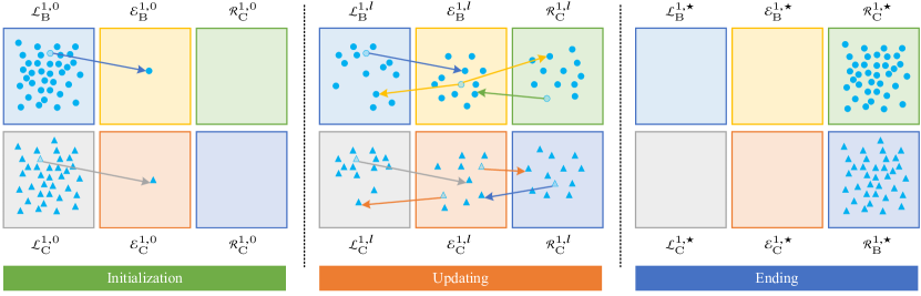
Figure 7: Illustration of our proposed solution path algorithm for the QPP (18): According to Theorem 3, all of samples in $\mathcal{B}$ initially locate in $\mathcal{L}_{\mathrm{B}}$ and $\mathcal{L}_{\mathrm{C}}$ when the regularization parameter $\lambda_{1}$ approaches infinity. Left: invoke Algorithm 1 to initialize the algorithm and obtain the initial index sets $\mathcal{L}_{\mathrm{B}}^{1,0},\mathcal{E}_{\mathrm{B}}^{1,0},\mathcal{R}_{\mathrm{B}}^{1,0},\mathcal{L}_{\mathrm{C}}^{1,0},\mathcal{E}_{\mathrm{C}}^{1,0},\mathcal{R}_{\mathrm{C}}^{1,0}$. Middle: invoke Algorithm 2 to update these parameters until the termination condition ends. Right: The ideal ending is that all of samples are located in $\mathcal{R}_{\mathrm{B}}$ and $\mathcal{R}_{\mathrm{C}}$.

For the QPP (18), it is also similar to the above.

4.4 Solution Path Algorithm

Our proposed solution path algorithm is illustrated in Figure 7. For the sample set with $K(K>3)$ classes, to obtain the entire solution path of regularization parameters $\lambda$, we need the following three steps.

Step 1: The data set is randomly divided into training set and test set, and the sampling rate of test samples is $r$.

Step 2: Any two categories of samples $K_{i}$ and $K_{j}~{}(i\neq j)$ are randomly selected from the training sample set, denoted as class $+1$ and $-1$, respectively, and the rest are denoted as class $0$. Sets of the three classes of samples are represented by $\mathcal{A}$, $\mathcal{B}$ and $\mathcal{C}$. Therefore, there are $K(K-2)/2$ combinations for samples with $K$ categories, and the optimal hyperplanes $f_{1,i,j}(\bm{x})$ and $f_{2,i,j}(\bm{x})$ corresponding to each combination $(K_{i},K_{j})$ are calculated respectively.

Step 2.1: For the QPP (3), there are two steps to the solution.

• Initialization: Set the initial value of system parameters $\delta$ and $\epsilon$, then invoke Algorithm 1 to determine the initial regularization parameter $\lambda_{1}^{0}$, the initial Lagrangian multipliers $\alpha_{i}^{0}$, $\beta_{k}^{0}$, the initial index sets $\mathcal{L}_{\mathrm{B}}^{1,0}$, $\mathcal{E}_{\mathrm{B}}^{1,0}$, $\mathcal{R}_{\mathrm{B}}^{1,0}$, $\mathcal{L}_{\mathrm{C}}^{1,0}$, $\mathcal{E}_{\mathrm{C}}^{1,0}$ and $\mathcal{R}_{\mathrm{C}}^{1,0}$.

• Updating: Invoke Algorithm 2 to get the entire solution to the QPP (3).

Step 2.2: For the QPP (18), there are two steps to the solution similar to the QPP (3).

Input: System parameters $\lambda_{\min}$ and $l_{\max}$, initial regularization parameter $\lambda_{1}^{0}$, initial Lagrangian multipliers $\alpha_{i}^{0}$, $\beta_{k}^{0}$, initial index sets $\mathcal{L}_{\mathrm{B}}^{1,0}$, $\mathcal{E}_{\mathrm{B}}^{1,0}$, $\mathcal{R}_{\mathrm{B}}^{1,0}$, $\mathcal{L}_{\mathrm{C}}^{1,0}$, $\mathcal{E}_{\mathrm{C}}^{1,0}$ and $\mathcal{R}_{\mathrm{C}}^{1,0}$.

Output: Solution path $\bm{\lambda}_{1}$, $\bm{\alpha}$ and $\bm{\beta}$.

1 $l\leftarrow 0$;

2 while $\lambda_{1}^{l}\geq\lambda_{\min}~{}\mathbf{and}~{}l\leq l_{\max}$  do

       $n_{\mathrm{B}}^{l}\leftarrow\mathrm{length}(\mathcal{E}_{\mathrm{B}}^{1,l})$, $n_{\mathrm{C}}^{l}\leftarrow\mathrm{length}(\mathcal{E}_{\mathrm{C}}^{1,l})$;

        // Number of samples in the elbow

3       Calculate $\bm{\theta}^{l}$ according to Equation 36;

       // Traverses through 8 defined events to see if they occur

4       foreach $e\in\{1,2,\cdots,8\}$ do

5             if event $e$ occurs then

6                   Obtain $\lambda_{1}^{e}$ according to Equations 55, 56, 57, 58, 59, 60, 61 and 62;

7                  

8            else

                   $\lambda_{1}^{e}\leftarrow 0$;

                    // Assign 0 if event $e$ doesn’t occur

9                  

10             end if

11            

12       end foreach

      // Update the iteration and the $(l+1)$-step parameters

       $\lambda_{1}^{l+1}\leftarrow\max\{\lambda_{1}^{1},\lambda_{1}^{2},\cdots,\lambda_{1}^{8}\}$;

        // Obtain the regularization parameter by Equation 63

       $e_{\mathrm{start}}\leftarrow\mathop{\arg\max}\{\lambda_{1}^{1},\lambda_{1}^{2},\cdots,\lambda_{1}^{8}\}$;

        // Determine which event occurs by Equation 64

13       Update $\mathcal{L}_{\mathrm{B}}^{1,l+1},\mathcal{E}_{\mathrm{B}}^{1,l+1},\mathcal{R}_{\mathrm{B}}^{1,l+1},\mathcal{L}_{\mathrm{C}}^{1,l+1},\mathcal{E}_{\mathrm{C}}^{1,l+1},\mathcal{R}_{\mathrm{C}}^{1,l+1}$ according to the event $e_{\mathrm{start}}$;

14       Update the Lagrangian multipliers $\alpha_{i}^{l+1}$, $\beta_{k}^{l+1}$ according to Theorem 1;

15       $l\leftarrow l+1$;

16      

17 end while

return $\bm{\lambda}_{1}$, $\bm{\alpha}$ and $\bm{\beta}$;

Algorithm 2 Traversal Search Algorithm of the QPP (3)

Step 3: To determine the optimal regularization parameter pairs $(\lambda,~{}\bar{\lambda})$ and its corresponding hyperplanes $f_{1,i,j}(\bm{x})$ and $f_{2,i,j}(\bm{x})$, the decision function $f_{i,j}(\bm{x})$ is utilized to evaluate the error for every combination $(K_{i},K_{j})$ on the examining set, and it generates ternary outputs $\{1,0,-1\}$.

$$f_{i,j}(\bm{x})=\left\{\begin{aligned} 1,~{}&\mathrm{if}~{}f_{1,i,j}(\bm{x})>-1+\epsilon,\\ -1,~{}&\mathrm{if}~{}f_{2,i,j}(\bm{x})<1-\epsilon,\\ 0,~{}&\mathrm{otherwise}.\end{aligned}\right.$$ (65)

Step 4: Predict the classes of samples in the test set using $K(K-2)/2$ pairs of the optimal regularization parameters. For any sample $\bm{x}$ in test set, we need to calculate its votes under the decision function $f_{i,j}(\bm{x})$.

• If $f_{1,i,j}(\bm{x})>-1+\epsilon$, then class $K_{i}$ gets “1” vote.

• If $f_{2,i,j}(\bm{x})<1-\epsilon$ and $f_{1,i,j}(\bm{x})<-1+\epsilon$, then class $K_{j}$ gets “1” vote.

• If $f_{1,i,j}(\bm{x})\leq-1+\epsilon$ or $f_{2,i,j}(\bm{x})\geq 1-\epsilon$, then both classes get “0” vote.

• If $f_{1,i,j}(\bm{x})>-1+\epsilon$ and $f_{2,i,j}(\bm{x})<1-\epsilon$, then both classes get “$-1$” vote.

Calculate the votes of $K$ classes of the sample under $K(K-2)/2$ decision functions, and the class with the most votes is its final category.

Table 1: Description of data sets used in this work.

No.	Data sets	# Tol.a	# Db	# Kc	# Size of classes
1	Balancescale	625	4	3	49, 288, 288
2	CMC	1473	9	3	629, 333, 511
3	Glass	214	9	6	29, 76, 70, 17, 13, 9
4	Iris	150	4	3	50, 50, 50
5	Robotnavigation	5456	24	4	826, 2097, 2205, 328
6	Seeds	210	7	3	70, 70, 70
7	Thyroid	215	5	3	150, 35, 30
8	Vowel	871	3	6	72, 89, 172, 151, 207, 180
9	Wine	178	13	3	59, 71, 48

• The total number of instances in the data set.

• The dimension of the features of the instance in the data set.

• The number of instance classes in the data set.

5 Numerical Experiments

In this section, we first verify the piecewise linear theory in Theorem 1 and 2 with experiments. We further test the proposed algorithm on prediction accuracy and training time in nine different data sets. The computational overhead and time complexity of the proposed algorithm are finally discussed.

5.1 Data Sets

According to the data sets in the relevant works (Xu et al., 2013; Ding et al., 2019), we have selected nine data sets with different feature dimensions, number of categories and total number of instances to evaluate the performance of the proposed algorithm. All the data sets can be achieved from the UCI machine learning repository, including Balancescale, CMC, Dermatology, Glass, Iris, Seeds, Thyroid, Vowel and Wine. And the detailed description, such as the size of classes of these data sets, is summarized in Table 1. The main goal of our work is to save parameter tuning time, so we deleted a few classes for some data sets. For instance, the original number of each class of data set Ecoli is 143, 77, 2, 2, 35, 20, 5 and 52 respectively. To reduce the cross-validation time, we can delete the classes with 3, 4 and 8 instances in the experiments.

5.2 Implementation Details

We compare against TSVM baselines with different strategies as in OVOVR TSVM (Xu et al., 2013), OVR TSVM (Cong et al., 2008) and OVO TSVM (Ding et al., 2019). We further compare against SVM baselines with different strategies as in OVR SVM (Angulo et al., 2003) and OVO SVM (Shieh & Yang, 2008). Note that all baselines are implemented based on the idea of multi-class strategies and the original TSVM/SVM. We closely follow the experimental setting in (Xu et al., 2013). On the large data sets, 10-fold cross-validation method is used to find the optimal parameters. Otherwise, we adopt leave-one method for validation. In the experiment, we set $r=0.25$, $\delta=10^{-4}$, $\epsilon=0.05$, $l_{\max}=1000$ and $\lambda_{\min}=10^{-4}$. For the vote strategy, we use two different decision functions to test ours and OVOVR TSVM. Furthermore, all the experiments are repeated ten times using the same parameter configuration.

For the grid search method, suppose the regularization parameter deduces from $\lambda=1000$, and the step is set to $\Delta\lambda=0.1$. We use the ‘quadprog.m’ function to realize the QPP in MATLAB.

All the experiments are performed by MATLAB R2016b on a personal computer equipped with an Intel (R) Core (TM) i7-7500U 2.90 GHz CPU and 8 GB memory capacity.

5.3 Results and Analysis

We first visualize a classification process and an entirely regularized solution path of two sub-optimization problems to verify the classification and pairwise linear theory, respectively. Then, we analyze the first event and compare the prediction accuracy performance and training time with state-of-the-art methods. Finally, we discuss the computational overhead and time complexity of TSVMPath.

5.3.1 Case Study

Visualization of classification results

To intuitively verify the correctness of our proposed algorithm, we first construct a handcrafted data set, including 3 classes with two-dimensional feature, and the test set is shown in Figure 8(a). Because it contains three classes, we need to evaluate three combinations as mentioned in Section 4.4, i.e., (1,2), (1, 3) and (2, 3). The corresponding results are depicted in Figures 8(d), 8(e) and 8(f), where samples in three classes are pinked into different colored markers and two non-parallel lines are shown in different colors. For example, Figure 8(f) illustrates the results of the combination (2,3). Three classes are shown in blue circles, red triangles and yellow pentagrams, labeled in “$-1$”, “0” and “$+1$”. Two non-parallel lines are shown in yellow and blue, which correspond to $w_{1}x_{1}+b_{1}=0$ and $w_{2}x_{2}+b_{2}=0$. Two decision boundaries $w_{1}x_{1}+b_{1}>-1+\epsilon$ and $w_{2}x_{2}+b_{2}<1-\epsilon$ divides the whole space to three areas w.r.t. three classes. The misclassified samples are marked by a green circle. As shown in Figure 8(f), the $+1$ area contains a misclassified sample and it achieves an accuracy of 99.3333%. The final results are shown in Figure 8(b), where our proposed algorithm achieves an accuracy of 99.3333%. However, the original OVOVR TSVM in Figure 8(c) only achieves an accuracy of 96.6667%, which is 2.6666% less than ours.

(a) Original Data

(b) Prediction (Ours)

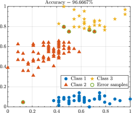
(c) Prediction (OVOVR TSVM)

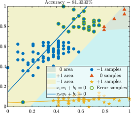
(d) (1,2)

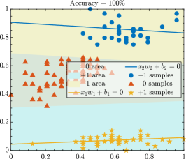
(e) (1,3)

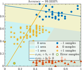
(f) (2,3)

Figure 8: Plots of classification results: (a) is the plot of original data with three classes; (b) and (c) are predicted results of ours and OVOVR TSVM; (d) to (f) are predicted results of three combinations (1,2), (1,3) and (2,3), respectively. (Best viewed in color.)

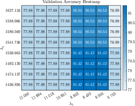
(a) CV (1,2)

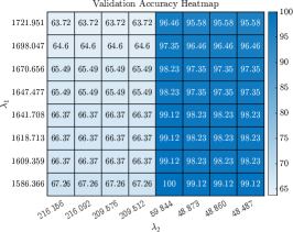
(b) CV (1,3)

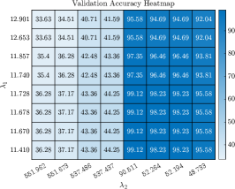
(c) CV (2,3)

Figure 9: Partial heatmaps of cross-validation accuracy: (a) to (c) are cross-validation heatmaps of three combinations (1,2), (1,3) and (2,3), respectively.

Otherwise, Figure 9 depicts the partial heatmaps of cross-validation accuracy for such three combinations. For example, Figure 9(c) shows the validation heatmap of the combination (2,3), where our proposed algorithm achieves the highest accuracy of 99.12% on the validation set. Notably, it achieves an accuracy of 99.3333% on the testing set, indicating the effectiveness of our proposed algorithm.

Visualization of piecewise linear solution path

Figures 10 and 11 show the entire solution path of the regularization parameter $\lambda_{1}$ for the QPP (3) and $\lambda_{2}$ for the QPP (18) on the data set Wine, where the regularization parameters are on the $log$ scale. Figures 10(a) and 11(a) depict the variation digram of regularization parameters $\lambda_{1}$ and $\lambda_{2}$, where it can be seen that the regularization parameters are reduced continuously to 0 with the step. Figures 10(b), 10(c), 11(b) and 11(c) are entire solutions of the Lagrangian multipliers $\bm{\alpha}$, $\bm{\beta}$, $\bm{\mu}$ and $\bm{\rho}$ respectively. For example, combining Figure 10(b) with Figure 10(a), it can be seen that the Lagrangian multipliers $\bm{\alpha}$ are piecewise linear w.r.t. the regularization parameter $\lambda_{1}$; combining Figure 11(b) with Figure 11(a), it can be seen that the Lagrangian multipliers $\bm{\mu}$ are piecewise linear w.r.t. the regularization parameter $\lambda_{1}$. Therefore, the piecewise linear theory established in Theorems 1 and 2 can be experimentally verified.

Additionally, Figures 10 and 11 also show the entire solution path of $\bm{f}$, $\bm{w}$ and $b$ w.r.t. two sub-optimization problems, respectively. For example, it can be seen from Figures 10(d) and 11(d) that the function values are distributed in different intervals. As mentioned in Section 4.4, when $f_{1}>-1+\epsilon$ in Figure 10(d), we can obtain the $+1$ samples. In the similar way, when $f_{2}<1-\epsilon$ in Figure 11(d), we can obtain the $-1$ samples. Combining Figure 10(d) with Figure 11(d), we can obtain the rest samples.

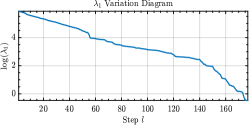
(a) $\lambda_{1}$

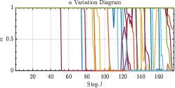
(b) $\bm{\alpha}$

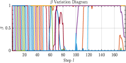
(c) $\bm{\beta}$

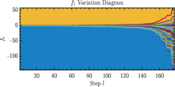
(d) $\bm{f}_{1}$

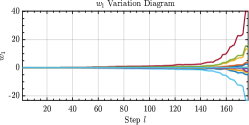
(e) $\bm{w}_{1}$

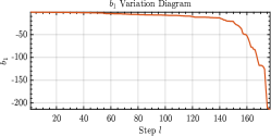
(f) $b_{1}$

Figure 10: An entire solution path of regularization parameters $\lambda_{1}$ and $\lambda_{2}$ on data set Wine for the first QPP: (a) to (f) are the plots of $\lambda_{1}$, $\bm{\alpha}$, $\bm{\beta}$, $\bm{f}_{1}$, $\bm{w}_{1}$ and $b_{1}$ respectively. (Note that $\lambda_{1}$ is on the $\log$ scale.)

(a) $\lambda_{2}$

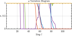
(b) $\bm{\alpha}$

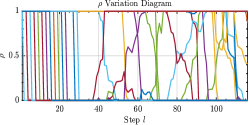
(c) $\bm{\beta}$

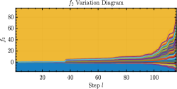
(d) $\bm{f}_{2}$

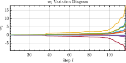
(e) $\bm{w}_{2}$

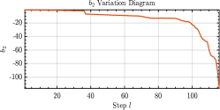
(f) $b_{2}$

Figure 11: An entire solution path on the data set Wine for the second QPP: (a) to (f) are the plots of $\lambda_{2}$, $\bm{\mu}$, $\bm{\rho}$, $\bm{f}_{2}$, $\bm{w}_{2}$ and $b_{2}$ respectively. (Note that $\lambda_{2}$ is on the $\log$ scale.)

5.3.2 Prediction Accuracy Results

Ours vs grid search method

Faced with the parameter tuning problem, one of the main strengths of the proposed algorithm is that we can search for an entire solution path in the parameter space whereas the grid search method can only find out limited solutions. Therefore, our prediction accuracy results on the same data set are better than the grid search method in most scenarios. Adopting the same data set division strategy on nine different data sets, we have tested the proposed algorithm and grid search method and the corresponding results are shown in Figure 12. Figure 12 to Figure 12 are plots on nine data sets respectively. In each plot, the solid red line with circle markers and the blue dotted line with square markers denote ours and the grid search method respectively. Note that we have repeated ten times on each data set using different data set divisions in order to ensure the reliability of the experiment. As can be seen in Figure 12, our prediction results are much better than the grid search method on several data sets such as CMC, Iris, Seeds, Robotnavigation and Vowel. For the other data sets, the prediction results for the two methods are about the same.

Other baselines

For the multi-classification problem, TSVM can be combined with different strategies. Note that the proposed algorithm is based on the OVOVR strategy. In this work, we compared our algorithm with OVO TSVM and OVR TSVM. Furthermore, SVM can be combined with OVO and OVR strategies to solve the multi-classification problems. Therefore, we have also tested OVO SVM and OVR SVM. The detailed results are elaborated in Table 2. Compared with other algorithms, the prediction accuracy of the proposed algorithm is better than other methods on dataset CMC, Iris, Robotnavigation, Seeds and Wine. For the data set Iris, Seeds and Wine, the number of samples in different categories is roughly the same. Therefore, the prediction accuracy is very high. However, the prediction accuracies of different algorithms are quite low for the data set CMC and Glass. The reason is that this data set may be linearly indivisible, while we use the linear kernel for all algorithms in this work. For data set Glass and Vowel with more than 3 classes, the prediction accuracy of ours and TSVM (OVOVR) are lower than other algorithms. It is demonstrated that the OVOVR strategy is slightly inferior compared with other strategies.

Although the prediction accuracy of our algorithm is not as good as that of other algorithms on some data sets, the prediction accuracy of our algorithm is generally superior to that of TSVM with the same OVOVR strategy as can be seen from Figure 12, indicating the effectiveness of our proposed solution path algorithm. We highlight that the main advantage of our algorithm is its low computational overhead and complexity with comparable results, while the performance lifting will be our future work. However, we have to admit that there are some limitations to the OVOVR strategy, e.g., cross-validation among different combinations is very time-consuming and the local optimal solution combination cannot always achieve the global optimal.

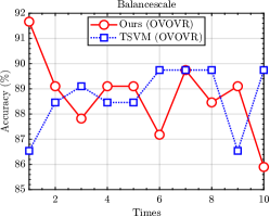
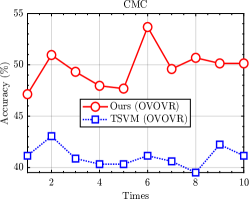
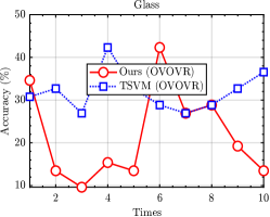
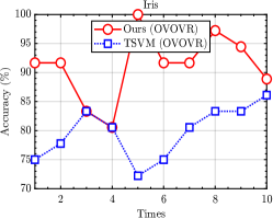
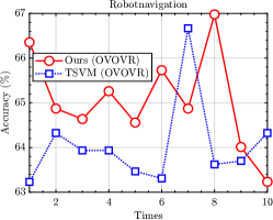
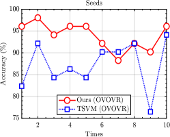
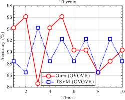
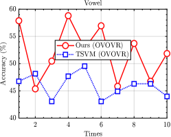
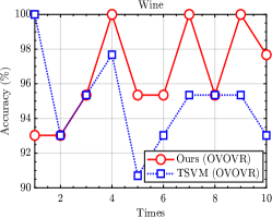
Figure 12: Prediction accuracy plots of ten times repeated experiments using ours and grid search method: (a) to (i) are prediction accuracy plots on each data set respectively; the solid red line with circles and the dotted line with squares denote the results of ours and the grid search method.

Table 2: Average prediction accuracy (%) of different algorithms on each data sets.

Data set	Ours (OVOVR)	TSVM (OVOVR)	TSVM (OVR)	TSVM (OVO)	SVM (OVR)	SVM (OVO)
	Acc, $\pm$ Std.	Acc, $\pm$ Std.	Acc, $\pm$ Std.	Acc, $\pm$ Std.	Acc, $\pm$ Std.	Acc, $\pm$ Std.
Balancescale	88.72 $\pm$ 1.55	88.65 $\pm$ 1.25	91.92 $\pm$ 2.44	88.21 $\pm$ 1.14	88.40 $\pm$ 1.61	91.47 $\pm$ 1.84
CMC	49.73 $\pm$ 1.90	41.04 $\pm$ 1.00	45.69 $\pm$ 1.07	43.92 $\pm$ 1.53	48.45 $\pm$ 1.96	51.36 $\pm$ 1.95
Glass	21.73 $\pm$ 10.88	31.92 $\pm$ 4.73	17.69 $\pm$ 7.73	32.69 $\pm$ 2.56	24.62 $\pm$ 4.42	39.23 $\pm$ 4.81
Iris	88.61 $\pm$ 7.23	79.72 $\pm$ 4.55	75.00 $\pm$ 7.52	96.39 $\pm$ 2.94	93.89 $\pm$ 4.10	98.33 $\pm$ 1.43
Robotnavigation	65.05 $\pm$ 1.09	64.05 $\pm$ 0.99	60.43 $\pm$ 2.81	60.38 $\pm$ 3.03	73.32 $\pm$ 1.34	75.07 $\pm$ 1.05
Seeds	93.92 $\pm$ 3.13	87.25 $\pm$ 5.49	92.16 $\pm$ 2.77	92.75 $\pm$ 1.61	92.35 $\pm$ 3.26	91.76 $\pm$ 4.01
Thyroid	91.15 $\pm$ 3.97	89.81 $\pm$ 2.73	83.27 $\pm$ 2.41	85.00 $\pm$ 4.33	95.96 $\pm$ 2.79	97.31 $\pm$ 3.03
Vowel	52.04 $\pm$ 4.95	45.97 $\pm$ 2.19	54.07 $\pm$ 1.82	53.56 $\pm$ 1.84	42.08 $\pm$ 13.42	81.67 $\pm$ 2.24
Wine	96.51 $\pm$ 2.74	94.88 $\pm$ 2.64	96.28 $\pm$ 2.94	94.65 $\pm$ 3.30	95.81 $\pm$ 2.14	95.58 $\pm$ 3.19

5.3.3 Training Time Comparison

The average training time of different algorithms is summarized in Table 3. In Table 3, we also list the average number of starting events of a solution path. Furthermore, Table 4 elaborates on the average number of starting events on each data set. The number of starting events reflects the size of the corresponding solution path. To save time, we just evaluate the training time of one solution for different algorithms. The proposed algorithm can be used to solve the entire solution path about regularization parameters. From Table 3, the training time of ours is quite less than that of the others. Since we do not need to solve any QPP to obtain the entire solution path, it can be seen from Table 3 that the time to solve QPP on the same data set is much longer than that of ours, the linear solving time. Therefore, the main factor restricting the training time is solving QPPs. The time to solve a QPP each time also depends on the size of the data set, and for high-dimensional data sets, the time to solve a QPP may even exceed a few hours. Therefore, the time of solving QPPs is used to measure the computational cost of different algorithms in this work.

Table 3: Average training time (s) of different algorithms on each data sets.

Data set	# Average starting events			Time a (s)	Training time of each solution (s)
	QPP (3)	QPP (18)	Total		Ours b (OVOVR)	TSVM (OVOVR)	TSVM (OVR)	TSVM (OVO)	SVM (OVR)	SVM (OVO)
Balancescale	517	731	1247	1.3149	0.0011	3.4525	0.8231	1.2516	0.0341	0.0331
CMC	1600	1053	2653	19.6988	0.0074	8.3385	4.5832	5.6763	2.4142	1.2867
Glass	2295	1587	3882	2.9809	0.0008	2.1671	0.4313	1.0795	0.0638	0.1211
Iris	122	123	245	0.7215	0.0029	0.1368	0.1049	0.1196	0.0266	0.0273
Robotnavigation	925	1000	1925	80.2642	0.0417	466.2647	239.3250	215.2090	21.2384	5.9840
Seeds	2880	1961	4841	0.5551	0.0001	0.1492	0.1428	0.1674	0.0278	0.0279
Thyroid	2974	2131	5105	0.4211	0.0001	0.2541	0.1876	0.2320	0.0762	0.0299
Vowel	3920	2957	6877	17.5491	0.0026	28.0308	7.9994	13.3788	53.1428	17.6766
Wine	178	209	387	0.8376	0.0022	0.1640	0.2616	0.1128	2.1981	0.9186

• Average training time of entire solution for ours.

• Average training time of each solution for ours.

Table 4: Average number of starting events on each data sets.

Data set	Event 1	Event 2	Event 3	Event 4	Event 5	Event 6	Event 7	Event 8	Sum
Balancescale	53	203	206	61	85	269	275	95	1247
CMC	68	389	399	90	221	587	745	154	2653
Glass	88	491	500	116	331	957	1133	267	3882
Iris	7	53	51	9	7	55	53	10	245
Robotnavigation	71	321	337	72	129	425	464	106	1925
Seeds	136	680	685	169	374	1147	1335	315	4841
Thyroid	147	746	751	179	384	1192	1380	327	5105
Vowel	185	928	936	227	499	1722	1927	453	6877
Wine	25	65	67	28	25	74	71	32	387

5.4 Discussion

In this section, we discuss the performance of the proposed algorithm in terms of the computational overhead and the time complexity, respectively.

Computational Overhead

Because the maximum regularization parameter $\lambda$ is reduced from 1000, and the step size of the regularization parameter $\lambda$ is $\Delta\lambda=0.1$ when the grid search method is adopted. Therefore, we need to solve $10^{8}$ QPPs in each combination $(K_{i},K_{j})$ for parameter tuning. In addition, we need to solve $\displaystyle K(K-1)\times 10^{8}$ QPPs to figure out the solution path. Due to the limitation of computing power, the grid search method cannot find the entire regularized solution path. Fortunately, the proposed solution path algorithm can expand the solution space of the regularized solution path to $(0,+\infty)$. Furthermore, no QPP is required for the proposed solution path algorithm. Since the training time of ours is linear, which is much less than that of solving QPP. Obviously, compared with the grid search method, the computational cost of the proposed algorithm will be greatly reduced. It can be seen that the proposed solution path algorithm has a significant advantage in parameter tuning.

Time Complexity

Since Algorithm 1 needs to solve linear equations of size $n_{B}+n_{C}$, its time complexity is $\mathcal{O}(\bar{n}^{2})$ at least where $\bar{n}$ denotes the average sample size. According to (Hastie et al., 2004), the time complexity of Algorithm 2 is $\mathcal{O}(c\bar{n}^{2}\bar{m}+\bar{n}\bar{m}^{2})$, where $\bar{m}$ is the average size of $\mathcal{E}_{\mathrm{B}}$ and $\mathcal{E}_{\mathrm{C}}$ and $c$ is a small number. In summary, the time complexity of the whole algorithm is proportional to the square of the data size. Additionally, the total computation burden of the entire solution path algorithm is similar to that of a single OVOVR TSVM fit. For example, Chen & Wu (2017) does not pay much attention to the complexity of parameter tuning, thus the classification accuracy can be guaranteed. They need to solve $K$ QPPs to obtain $K$ hyperplanes for the multi-classification problem, which is more expensive than ours. For the grid search method, we need to fit the OVOVR TSVM $n_{\mathrm{grid}}$ times, and the corresponding time complexity is also $n_{\mathrm{grid}}$ times of OVOVR TSVM fits, where $n_{\mathrm{grid}}$ is the granularity of the grid, e.g., $n_{\mathrm{grid}}$ is equal to $2\times 10^{4}$ as analyzed above in this work. Therefore, the solution path algorithm can greatly reduce the computational burden of parameter adjustment, with up to four orders of magnitude speed-up for the computational complexity compared with the grid search method. Furthermore, the convergence of solution path algorithm can be guaranteed by Hastie et al. (2004).

6 Conclusion

In this work, the twin multi-class SVM with the OVOVR strategy is studied and its fast regularization parameter tuning algorithm is developed. The solutions of the two sub-optimization problems are proved to be piecewise linear on the regularization parameters, and the entire regularized solution path algorithm is developed accordingly. The simulation results on UCI data sets show that the Lagrangian multipliers are piecewise linear w.r.t. the regularization parameters of the two sub-models, which lays a foundation for further selecting regularization parameters and makes the generalization performance of the twin multi-class support vector machine better. It should be noted that no QPP is involved in the proposed algorithm, thus sharply reducing the computational cost.

References

- Angulo et al. (2003) Angulo, C., Xavier, P., & Andreu, C. (2003). K-svcr. a support vector machine for multi-class classification. Neurocomputing, 55, 57–77. doi:https://doi.org/10.1016/S0925-2312(03)00435-1.
- Bai et al. (2019) Bai, L., Shao, Y., Wang, Z., & Li, C. (2019). Clustering by twin support vector machine and least square twin support vector classifier with uniform output coding. Knowledge-Based Systems, 163, 227–240. doi:https://doi.org/10.1016/j.knosys.2018.08.034.
- Chen & Wu (2017) Chen, S.-G., & Wu, X.-J. (2017). Multiple birth least squares support vector machine for multi-class classification. International Journal of Machine Learning and Cybernetics, 8, 1731–1742. doi:https://doi.org/10.1007/s13042-016-0554-7.
- Chen et al. (2011) Chen, X., Yang, J., Ye, Q., & Liang, J. (2011). Recursive projection twin support vector machine via within-class variance minimization. Pattern Recognition, 44, 2643–2655. doi:https://doi.org/10.1016/j.patcog.2011.03.001.
- Cong et al. (2008) Cong, H., Yang, C., & Pu, X. (2008). Efficient speaker recognition based on multi-class twin support vector machines and gmms. In 2008 IEEE conference on robotics, automation and mechatronics (pp. 348–352). IEEE. doi:https://doi.org/10.1109/RAMECH.2008.4681433.
- Cortes & Vapnik (1995) Cortes, C., & Vapnik, V. (1995). Support-vector networks. Machine Learning, 20, 273–297. doi:https://doi.org/10.1023/A:1022627411411.
- Crammer & Singer (2002) Crammer, K., & Singer, Y. (2002). On the learnability and design of output codes for multiclass problems. Machine learning, 47, 201–233. doi:https://doi.org/10.1023/A:1013637720281.
- Ding et al. (2019) Ding, S., Zhao, X., Zhang, J., Zhang, X., & Xue, Y. (2019). A review on multi-class twsvm. Artificial Intelligence Review, 52, 775–801. doi:https://doi.org/10.1007/s10462-017-9586-y.
- Gu & Sheng (2017) Gu, B., & Sheng, V. (2017). A robust regularization path algorithm for -support vector classification. IEEE transactions on Neural Networks and Learning Systems, 28, 1241–1248. doi:https://doi.org/10.1109/tnnls.2016.2527796.
- Hastie et al. (2004) Hastie, T., Rosset, S., Tibshirani, R., & Zhu, J. (2004). The entire regularization path for the support vector machine. Journal of Machine Learning Research, 5, 1391–1415. URL: https://www.jmlr.org/papers/volume5/hastie04a/hastie04a.pdf.
- Hsieh & Yeh (2011) Hsieh, T., & Yeh, W. (2011). Knowledge discovery employing grid scheme least squares support vector machines based on orthogonal design bee colony algorithm. IEEE Transactions on Systems, Man, and Cybernetics, 41, 1198–1212. doi:https://doi.org/10.1109/tsmcb.2011.2116007.
- Hsu & Lin (2002) Hsu, C., & Lin, C. (2002). A comparison of methods for multiclass support vector machines. IEEE transactions on Neural Networks, 13, 415–25. doi:https://doi.org/10.1109/72.991427.
- Hu et al. (2013) Hu, L., Lu, S., & Wang, X. (2013). A new and informative active learning approach for support vector machine. Information Sciences, 244, 142–160. doi:https://doi.org/10.1016/j.ins.2013.05.010.
- Huang et al. (2017) Huang, X., Shi, L., & Suykens, J. (2017). Solution path for pin-svm classifiers with positive and negative values. IEEE transactions on Neural Networks and Learning Systems, 28, 1584–1593. doi:https://doi.org/10.1109/tnnls.2016.2547324.
- Jayadeva et al. (2007) Jayadeva, Khemchandani, R., & Chandra, S. (2007). Twin support vector machines for pattern classification. IEEE Transactions on Pattern Analysis and Machine Intelligence, 29, 905–910. doi:https://doi.org/10.1109/TPAMI.2007.1068.
- KreBel (1999) KreBel, U. H.-G. (1999). Pairwise classification and support vector machines. In Advances in Kernel Methods: Support Vector Learning (p. 255–268). Cambridge, MA, USA: MIT Press.
- Kumar & Gopal (2009) Kumar, M., & Gopal, M. (2009). Least squares twin support vector machines for pattern classification. Expert Systems with Applications, 36, 7535–7543. doi:https://doi.org/10.1016/j.eswa.2008.09.066.
- Lee & Lee (2005) Lee, J., & Lee, D. (2005). An improved cluster labeling method for support vector clustering. IEEE Transactions on Pattern Analysis and Machine Intelligence, 27, 461–464. doi:https://doi.org/10.1109/tpami.2005.47.
- Li et al. (2017) Li, J., Cao, Y., Wang, Y., & Xiao, H. (2017). Online learning algorithms for double-weighted least squares twin bounded support vector machines. Neural Processing Letters, 45, 319–339. doi:https://doi.org/10.1007/s11063-016-9527-9.
- Li et al. (2021) Li, J., Zhou, K., & Mu, B. (2021). Machine learning for mass spectrometry data analysis in proteomics. Current Proteomics, 18, 620–634. doi:https://doi.org/10.2174/1570164617999201023145304.
- de Lima et al. (2018) de Lima, M., Costa, N., & Barbosa, R. (2018). Improvements on least squares twin multi-class classification support vector machine. Neurocomputing, 313, 196–205. doi:https://doi.org/10.1016/j.neucom.2018.06.040.
- López et al. (2016) López, J., Maldonado, S., & Carrasco, M. (2016). A novel multi-class svm model using second-order cone constraints. Applied Intelligence, 44, 457–469. doi:https://doi.org/10.1007/s10489-015-0712-8.
- Luo et al. (2020) Luo, J., Yan, X., & Tian, Y. (2020). Unsupervised quadratic surface support vector machine with application to credit risk assessment. European Journal of Operational Research, 280, 1008–1017. doi:https://doi.org/10.1016/j.ejor.2019.08.010.
- Ogawa et al. (2013) Ogawa, K., Suzuki, Y., & Takeuchi, I. (2013). Safe screening of non-support vectors in pathwise svm computation. In Proceedings of the 30th International Conference on Machine Learning (pp. 1382–1390). Atlanta, GA, USA.
- Ong et al. (2010) Ong, C., Shao, S., & Yang, J. (2010). An improved algorithm for the solution of the regularization path of support vector machine. IEEE transactions on Neural Networks, 21, 451–462. doi:https://doi.org/10.1109/tnn.2009.2039000.
- Pan et al. (2017) Pan, X., Yang, Z., Xu, Y., & Wang, L. (2017). Safe screening rules for accelerating twin support vector machine classification. IEEE transactions on neural networks and learning systems, 29, 1876–1887. doi:https://doi.org/10.1109/tnnls.2017.2688182.
- Pang et al. (2019) Pang, X., Pan, X., & Xu, Y. (2019). Multi-parameter safe sample elimination rule for accelerating nonlinear multi-class support vector machines. Pattern Recognition, 95, 1–11. doi:https://doi.org/10.1016/j.patcog.2019.05.037.
- Pang et al. (2018) Pang, X., Xu, C., & Xu, Y. (2018). Scaling knn multi-class twin support vector machine via safe instance reduction. Knowledge-Based Systems, 148, 17–30. doi:https://doi.org/10.1016/j.knosys.2018.02.018.
- Shieh & Yang (2008) Shieh, M.-D., & Yang, C.-C. (2008). Multiclass svm-rfe for product form feature selection. Expert Systems with Applications, 35, 531–541.
- Sun (2011) Sun, S. (2011). Multi-view laplacian support vector machines. In International Conference on Advanced Data Mining and Applications (pp. 209–222). Springer. doi:https://doi.org/10.1007/s10489-014-0563-8.
- Sun & Xie (2015) Sun, S., & Xie, X. (2015). Semisupervised support vector machines with tangent space intrinsic manifold regularization. IEEE transactions on Neural Networks and Learning Systems, 27, 1827–1839. doi:https://doi.org/10.1109/tnnls.2015.2461009.
- Sun et al. (2018) Sun, S., Xie, X., & Dong, C. (2018). Multiview learning with generalized eigenvalue proximal support vector machines. IEEE transactions on cybernetics, 49, 688–697. doi:https://doi.org/10.1109/tcyb.2017.2786719.
- Sun et al. (2019) Sun, X., Su, S., Huang, Z., Zuo, Z., Guo, X., & Wei, J. (2019). Blind modulation format identification using decision tree twin support vector machine in optical communication system. Optics Communications, 438, 67–77. doi:https://doi.org/10.1016/j.optcom.2019.01.025.
- Tanveer et al. (2016) Tanveer, M., Khan, M., & Ho, S. (2016). Robust energy-based least squares twin support vector machines. Applied Intelligence, 45, 174–186. doi:https://doi.org/10.1007/s10489-015-0751-1.
- Tomar & Agarwal (2015) Tomar, D., & Agarwal, S. (2015). A comparison on multi-class classification methods based on least squares twin support vector machine. Knowledge-Based Systems, 81, 131–147. doi:https://doi.org/10.1016/j.knosys.2015.02.009.
- Vaidya et al. (2008) Vaidya, J., Yu, H., & Jiang, X. (2008). Privacy-preserving svm classification. Knowledge and Information Systems, 14, 161–178. doi:https://doi.org/10.1007/s10115-007-0073-7.
- Wang et al. (2008a) Wang, G., Yeung, D., & Lochovsky, F. (2008a). A new solution path algorithm in support vector regression. IEEE transactions on Neural Networks, 19, 1753–1767. doi:https://doi.org/10.1109/tnn.2008.2002077.
- Wang et al. (2006) Wang, G., Yeung, D.-Y., & Lochovsky, F. H. (2006). Two-dimensional solution path for support vector regression. In Proceedings of the 23rd international conference on Machine learning (pp. 993–1000). doi:http://dx.doi.org/10.1145/1143844.1143969.
- Wang & Zhang (2021) Wang, H., & Zhang, Q. (2021). Twin k-class support vector classification with pinball loss. Applied Soft Computing, 113, 107929. doi:https://doi.org/10.1016/j.asoc.2021.107929.
- Wang et al. (2018) Wang, H., Zhou, Z., & Xu, Y. (2018). An improved -twin bounded support vector machine. Applied Intelligence, 48, 1041–1053. doi:https://doi.org/10.1007/s10489-013-0500-2.
- Wang et al. (2008b) Wang, L., Zhu, J., & Zou, H. (2008b). Hybrid huberized support vector machines for microarray classification and gene selection. Bioinformatics, 24, 412–419. doi:https://doi.org/10.1093/bioinformatics/btm579.
- Weston & Watkins (1999) Weston, J., & Watkins, C. (1999). Support vector machines for multi-class pattern recognition. In Proceedings of the 7th European Symposium on Artificial Neural Networks (pp. 219–224). volume 99.
- Xie et al. (2013) Xie, J., Hone, K., Xie, W., Gao, X., Shi, Y., & Liu, X. (2013). Extending twin support vector machine classifier for multi-category classification problems. Intelligent Data Analysis, 17, 649–664. doi:http://dx.doi.org/10.3233/IDA-130598.
- Xie & Sun (2014) Xie, X., & Sun, S. (2014). Multi-view laplacian twin support vector machines. Applied Intelligence, 41, 1059–1068. doi:https://doi.org/10.1007/s10489-014-0563-8.
- Xie & Sun (2020) Xie, X., & Sun, S. (2020). Multi-view support vector machines with the consensus and complementarity information. IEEE Transactions on Knowledge and Data Engineering, 32, 2401–2413. doi:https://doi.org/10.1109/TKDE.2019.2933511.
- Xie et al. (2018) Xie, X., Sun, S., Chen, H., & Qian, J. (2018). Domain adaptation with twin support vector machines. Neural Processing Letters, 48, 1213–1226. doi:https://doi.org/10.1007/s11063-017-9775-3.
- Xu (2016) Xu, Y. (2016). K-nearest neighbor-based weighted multi-class twin support vector machine. Neurocomputing, 205, 430–438. doi:https://doi.org/10.1016/j.neucom.2016.04.024.
- Xu et al. (2015) Xu, Y., Pan, X., Zhou, Z., Yang, Z., & Zhang, Y. (2015). Structural least squares twin support vector machine for classification. Applied Intelligence, 42, 527–536. doi:https://doi.org/10.1016/j.knosys.2013.01.008.
- Xu et al. (2013) Xu, Y., Rui, G., & Wang, L. (2013). A twin multi-class classification support vector machine. Cognitive Computation, 5, 580–588. doi:https://doi.org/10.1007/s12559-012-9179-7.
- Yang et al. (2015) Yang, J., Gong, L., Tang, Y., Yan, J., He, H., Zhang, L., & Li, G. (2015). An improved svm-based cognitive diagnosis algorithm for operation states of distribution grid. Cognitive Computation, 7, 582–593. doi:https://doi.org/10.1007/s12559-015-9323-2.
- Yang et al. (2018) Yang, Z., Pan, X., & Xu, Y. (2018). Piecewise linear solution path for pinball twin support vector machine. Knowledge-Based Systems, 160, 311–324. doi:https://doi.org/10.1016/j.knosys.2018.07.022.
- Yang et al. (2013) Yang, Z., Shao, Y., & Zhang, X. (2013). Multiple birth support vector machine for multi-class classification. Neural Computing and Applications, 22, S153–S161. doi:https://doi.org/10.1007/s00521-012-1108-x.
- Ye et al. (2012) Ye, Q., Zhao, C., Gao, S., & Zheng, H. (2012). Weighted twin support vector machines with local information and its application. Neural Networks, 35, 31–39. doi:https://doi.org/10.1016/j.neunet.2012.06.010.
- Zhang et al. (2016) Zhang, X., Ding, S., & Sun, T. (2016). Multi-class lstmsvm based on optimal directed acyclic graph and shuffled frog leaping algorithm. International Journal of Machine Learning and Cybernetics, 7, 241–251. doi:https://doi.org/10.1007/s13042-015-0435-5.
- Zhang et al. (2014) Zhang, Y., Fu, P., Liu, W., & Chen, G. (2014). Imbalanced data classification based on scaling kernel-based support vector machine. Neural Computing and Applications, 25, 927–935. doi:https://doi.org/10.1007/s00521-014-1584-2.
- Zhou et al. (2022) Zhou, K., Zhang, Q., & Li, J. (2022). Tsvmpath: Fast regularization parameter tuning algorithm for twin support vector machine. Neural Processing Letters, (pp. 1–26). doi:https://doi.org/10.1007/s11063-022-10870-1.
- Zhou & Liu (2005) Zhou, Z.-H., & Liu, X.-Y. (2005). Training cost-sensitive neural networks with methods addressing the class imbalance problem. IEEE Transactions on knowledge and data engineering, 18, 63–77. doi:https://doi.org/10.1109/TKDE.2006.17.