Sufficient Dimension Reduction for Interactions

Abstract

Dimension reduction lies at the heart of many statistical methods. In regression, dimension reduction has been linked to the notion of sufficiency whereby the relation of the response to a set of predictors is explained by a lower dimensional subspace in the predictor space. In this paper, we consider the notion of a dimension reduction in regression on subspaces that are sufficient to explain interaction effects between predictors and another variable of interest. The motivation for this work is from precision medicine where the performance of an individualized treatment rule, given a set of pretreatment predictors, is determined by interaction effects.

Keywords: Precision medicine, modified covariate method, projection-pursuit regression, single-index models, central mean subspace

1 INTRODUCTION

The notion of sufficiency, introduced by Fisher (Fisher, 1922), plays a fundamental role in statistics. A statistic is sufficient if it summarizes all the relevant information in the sample about the parameter of interest. Sufficiency can be regarded as a form of dimension reduction whereby a sample of size $n$ is reduced to a low-dimension statistic. Cook (Cook, 2007, Section 8.2) extended the notion of sufficiency to the realm of regression as a dimension reduction concept (see also, Cook, 1994, 1996; Li, 1991, 1992; Bura and Cook, 2001; Adragni and Cook, 2009). Given a set of $p$ covariates $\bm{X}\in\mathbb{R}^{p}$ and an outcome variable $Y\in\mathbb{R}$, Cook’s notion of a sufficient subspace in regression can be summarized as $Y|\bm{X}\sim Y|R(\bm{X})$ where $R:\mathbb{R}^{p}\mapsto\mathbb{R}^{q},\;q<p$.

The central subspace, which is denoted by $S_{Y\mid\bm{X}}$, is the subspace with the smallest possible dimension $q$ in $\mathbb{R}^{p}$, such that $Y$ is independent of $\bm{X}$ given $R(\bm{X})=\bm{B}^{\top}\bm{X}$ for some $p\times q$ matrix $\bm{B}$, $q<p$, where the columns of $\bm{B}$ form a basis for the subspace (Cook and Li, 2002). For comprehensive discussion, see (Cook, 1998). Dimension reduction is often aimed at reducing dimensionality for modeling the conditional mean function $\mathbb{E}[Y|\bm{X}]$ alone, while leaving the rest of the distribution $Y|\bm{X}$ as the “nuisance parameter.” For this case, Cook and Li (Cook and Li, 2002) introduced the central mean subspace, denoted as $S_{\mathbb{E}[Y\mid\bm{X}]}$, defined to be the smallest subspace, $\mbox{span}(\bm{B})$ for some basis matrix $\bm{B}$, sufficient to model the conditional mean $\mathbb{E}[Y|\bm{X}]$.

In this paper, we extend the notion of a sufficient subspace in regression with an outcome variable $Y$ when our interest is in the interaction effect between the vector of covariates $\bm{X}$ and another variable $A\in\mathcal{A}$. This paper considers the case when $A$ is a discrete random variable on a space $\mathcal{A}=\{1,\ldots,L\}$, i.e., there are $L$ possible levels for the random variable $A$; however, the notion will also be extended to a continuous compact interval $\mathcal{A}\subset\mathbb{R}$. The primary focus is on reducing the dimension of $\bm{X}$ to model the effects of interactions between $\bm{X}$ and $A$ on $Y$. The motivation for this work is in the context of precision medicine, where we seek to optimize an individualized treatment rule that assigns a treatment to each patient according to the patient’s specific characteristics, in the hope of improving efficacy of treatments and lowering medical cost. Typically, individual-specific medical/clinical characteristics are represented by a vector of covariates $\bm{X}$ measured before treatment assignment, and treatment condition can be represented by the variable $A$. An optimal individualized treatment rule is solely determined by the $\bm{X}$-by-$A$ interaction effects on $Y$ (e.g., see Qian and Murphy, 2011). Therefore, a sufficient reduction subspace for $\bm{X}$ in this setting will typically be defined in terms of a subspace sufficient to model the $\bm{X}$-by-$A$ interaction effect, whereas the pure main effect for $\bm{X}$ on $Y$ will be viewed as a “nuisance” effect.

In this paper, we define a sufficient dimension reduction subspace for $\bm{X}$ in terms of a parsimonious characterization of the $\bm{X}$-by-$A$ interaction effect available from $\mathbb{E}[Y|\bm{X},A]$, and we introduce a semiparametric framework for producing a basis $\bm{B}$ for such sufficient subspace. The proposed framework of modeling the $\bm{X}$-by-$A$ interactions takes the linear model based approaches (e.g., Tian et al., 2014; Lu et al., 2011; Shi et al., 2016, 2018; Jeng et al., 2018) as its special cases. Luo, et al. (Luo et al., 2018) considered sufficient dimension reduction to estimate a lower dimensional linear combination of $\bm{X}$ that is sufficient to model the regression causal effect, defined as the mean difference in the potential outcomes (Rubin, 1974) conditional on $\bm{X}$ (see also, Luo et al., 2017), when the treatment variable $A$ is binary-valued. Our framework, instead, focuses on the interaction between treatment and covariates, allows $L$ treatment levels, and it can be easily modified to incorporate the case where $A$ is defined on a continuum.

2 SUFFICIENT REDUCTION FOR INTERACTIONS

2.1 PRELIMINARIES

Our approach to the sufficient reduction for interactions is to express the conditional expectation function $\mathbb{E}[Y|\bm{X},A]$ in terms of a main effect for $\bm{X}$ and a $\bm{X}$-by-$A$ interaction effect. Consider the following decomposition of the conditional expectation:

$$\mathbb{E}[Y|\bm{X},A]\ =\ \mu(\bm{X})+g(\bm{X},A),$$ (2.1)

where the first term $\mu(\bm{X})$ does not depend on $A$ and only the second term $g(\bm{X},A)$ is a function of $A$. Under representation (2.1), the marginal effect of $\bm{X}$ on $Y$ is expressed as:

$$\mathbb{E}[Y\mid\bm{X}] = \mathbb{E}[\mathbb{E}[Y\mid\bm{X},A]\mid\bm{X}]$$

$$= \mathbb{E}[\mu(\bm{X})+g(\bm{X},A)\mid\bm{X}]$$

$$= \mu(\bm{X})+\mathbb{E}[g(\bm{X},A)\mid\bm{X}]$$

In what follows, for the identifiability of decomposition (2.1), we will set

$$\mathbb{E}[g(\bm{X},A)|\bm{X}]=0.$$ (2.2)

The condition (2.2) implies that, in (2.1), the first term $\mu(\bm{X})=\mathbb{E}[Y|\bm{X}]$ represents the $\bm{X}$ marginal effect, and the second term $g(\bm{X},A)$ represents the “pure” $\bm{X}$-by-$A$ interaction effect. Throughout the paper, we write $\bm{\Sigma}=\mbox{var}(\bm{X})$, and assume an additive mean zero noise with finite variance.

2.2 CENTRAL MEAN SUBSPACE

For a discrete treatment space $\mathcal{A}=\{1,\dots,L\}$ with $L$ available treatments, a treatment decision function, $\mathcal{D}(\bm{X}):\mathbb{R}^{p}\mapsto\mathcal{A}$, mapping each individual’s pretreatment covariates $\bm{X}\in\mathbb{R}^{p}$ to one of the $L$ treatment options, defines an individualized treatment rule (Murphy, 2003; Robins, 2004; Zhang et al., 2012; Cai et al., 2011; Qian and Murphy, 2011) for s single decision time point. The average outcome when all individuals are treated according to such rule is referred to as the “value” $(V)$ of the individualized treatment rule (Qian and Murphy, 2011), which can be expressed as $V(\mathcal{D})=\mathbb{E}[\mathbb{E}[Y|\bm{X},A=\mathcal{D}(\bm{X})]]$. Without loss of generality, if we assume a larger value of $Y$ is desirable, then it is straightforward to verify that the optimal individualized treatment rule, $\mathcal{D}^{opt}$, which results in the largest value $V(\mathcal{D}^{opt})$, is of the form:

$$\mathcal{D}^{opt}(\bm{X})\ =\ \operatorname*{arg\,max}_{a\in\mathcal{A}}\ \mathbb{E}\big{[}Y|\bm{X},A=a\big{]},$$ (2.3)

i.e., the optimal individualized treatment rule assigns a treatment to an individual patient based on the highest expected quality treatment given $\bm{X}$.

We will cast the notion of sufficient reduction for $\bm{X}$-by-$A$ interaction effects under the general representation (2.1). We define a contrast vector $\bm{c}=(c_{1},\ldots,c_{L})^{\top}\in\mathbb{R}^{L}$ as a vector such that $\sum_{a=1}^{L}{c_{a}}=0$ (zero-sum constraint) and $\bm{c}\neq(0,\ldots,0)^{\top}$, i.e., $\bm{c}$ is not a vector of all zeros (to avoid the trivial case).

Definition 1.

For an arbitrary contrast vector $\bm{c}=(c_{1},\ldots,c_{L})^{\top}$, we define the mean contrast function of $\bm{X}$, as the following linear combination:

$$\mathcal{C}(\bm{X};{\bm{c}}):=\sum_{a=1}^{L}c_{a}\mathbb{E}\left[Y|\bm{X},A=a\right].$$ (2.4)

The mean contrast function (2.4) is a transformation of the function $\mathbb{E}\left[Y|\bm{X},A\right]$ in (2.1) from its original domain $(\bm{X},A)$ to the new domain $(\bm{X},\bm{c})$. The condition $\sum_{a=1}^{L}c_{a}=0$ imposed on $\bm{c}$ makes the $\bm{X}$ marginal effect $\mu(\bm{X})$ in the general model (2.1) drop out from $\mathcal{C}(\bm{X};{\bm{c}})$ in (2.4). As a result, the mean contrast function (2.4), for any $\bm{c}$, is independent of the marginal effect $\mu(\bm{X})$ in (2.1).

In a treatment context, $\mathcal{C}(\bm{X};\bm{c})$ is a measure comparing individualized efficacies of treatments for a given contrast $\bm{c}$, as a function of the pretreatment covariates $\bm{X}$. For example, if $L=2$, the optimal individualized treatment rule defined in (2.3) is determined by the sign of $\mathcal{C}(\bm{X};\bm{c})$ when $c_{1}=1$ and $c_{2}=-1$, and (2.4) is reduced to the case studied by Luo, et al. (Luo et al., 2018).

In this paper, we consider a lower dimensional transformation of $\bm{X}$ that is sufficient to recover the mean contrast functions $\mathcal{C}(\bm{X};\bm{c})$ in (2.4), for any contrast vector $\bm{c}$.

Definition 2.

Let $\bm{B}$ denote a $p\times q$ matrix with full column rank. The transformation $R(\bm{X})=\bm{B}^{\top}\bm{X}$ is said to be a sufficient dimension reduction for $\bm{X}$-by-$A$ interactions, if

$$\mathcal{C}(\bm{X};\bm{c})=\mathcal{C}(\bm{B}^{\top}\bm{X};\bm{c})=\sum_{a=1}^{L}c_{a}g_{a}(\bm{B}^{\top}\bm{X})$$ (2.5)

for any contrast vector $\bm{c}$, where the functions $\{g_{a}\}_{a\in\mathcal{A}}$ are unspecified functions associated with each level of $A\in\mathcal{A}$ defined on $\bm{B}^{\top}\bm{X}\in\mathbb{R}^{q}$. The column space of $\bm{B}$ will be called a sufficient reduction subspace for $\bm{X}$-by-$A$ interactions.

For any $p\times q$ matrix $\bm{B}=(\bm{\beta};\ldots;{\bm{\beta}}_{q})$ satisfying (2.5) and any $p\times p$ nonsingular matrix $\bm{\eta}$, $\bm{\eta}\bm{B}$ still satisfies (2.5) when the $\{g_{a}\}_{a\in\mathcal{A}}$ are adjusted accordingly. A further constraint on $\bm{B}$ is needed for an identifiable parametrization. To remove trivial ambiguity, let us define a set of $p\times q$ matrices, denoted as $\Theta_{q}$, that have a positive first nonzero entry and consists of $q$ distinct orthonormal vectors; in (2.5), without loss of generality, we assume $\bm{B}\in\Theta_{q}$.

As the notion of sufficiency (2.5) is based on the contrast function $\mathcal{C}(\bm{X};\bm{c})$ that is independent of $\mu(\bm{X})$ in (2.1), we can formalize a minimally sufficient dimension reduction in $\bm{X}$ specifically for the term $g(\bm{X},A)$ in (2.1).

Definition 3.

A sufficient reduction subspace for interactions is said to be minimal, if the dimension of its span is less than or equal to the dimension of the span of any other sufficient reduction subspace for interactions. We denote the minimally sufficient reduction subspace (also called the central mean subspace) for $\bm{X}$-by-$A$ interactions as $S_{\mathcal{C}|\bm{X}}$, and $\mbox{dim}(S_{\mathcal{C}|\bm{X}})$ will denote its dimension.

The central mean subspace of Cook and Li (2002) refers to the minimally sufficient subspace in $\mathbb{R}^{p}$ associated with the mean response function. The subspace $S_{\mathcal{C}|\bm{X}}$ is a special case of the central mean subspace for the mean function (2.1) in which only the interaction term $g(\bm{X},A)$ is considered for dimension reduction. We assume that the central mean subspace for interactions, $S_{\mathcal{C}|\bm{X}}$, uniquely exists throughout this article. The uniqueness of the central mean subspace is guaranteed under fairly general conditions (Cook and Li, 2002; Luo et al., 2018; Yin et al., 2008); for example, it is guaranteed when the domain of $\bm{X}$ is open and convex.

Remark 2.1.

If there exists a $p\times q$ dimension reduction matrix $\bm{B}$ with $q<p$ such that $\mathcal{C}(\bm{X};\bm{c})=\mathcal{C}(\bm{B}^{\top}\bm{X};\bm{c})$, the corresponding transformation is sufficient (for interactions) based on Definition 2, but this need not be a minimal sufficient reduction. For example, if $\bm{X}=(X_{1},X_{2})^{\top}$ and $\mathbb{E}[Y|\bm{X},A=a]=X_{1}+\gamma_{a}X_{2}$ $(a\in\mathcal{A})$ (for $\gamma_{a}\in\mathbb{R}$ and $\mbox{var}(\gamma_{A})>0$), then the $2\times 2$ identity matrix $\bm{B}=\begin{pmatrix}1&0\\ 0&1\\ \end{pmatrix}$ corresponds to a sufficient reduction, but the minimal sufficient reduction is determined by the vector $\bm{B}=(0,1)^{\top}\in\Theta_{1}$, since the effect of $A$ is a function only of $X_{2}$ and does not depend on $X_{1}$.

Dimension reduction using a minimal number, $\mbox{dim}(S_{\mathcal{C}|\bm{X}})$, of directions is important for interpretability and parsimonious parametrization, and allows a more accurate estimation. In practice, 1-dimensional reductions often suffice in capturing pertinent interaction effects and are typically of primary interest. Examples of 1-dimensional reductions include performing a regression with a linear model that focuses on a single vector of coefficients (e.g., Tian et al., 2014; Petkova et al., 2016) and its semiparametric generalization with a set of flexible link functions, a single-index model with treatment level-specific link functions (Park et al., 2020b). In the remainder of the paper, we introduce a semiparametric regression framework for approximating the minimally sufficient subspace $S_{\mathcal{C}|\bm{X}}$ for $\bm{X}$-by-$A$ interactions and build connections to other linear model-based approaches as its special cases.

2.3 THE MODEL

Motivated by the notion of sufficiency (2.5), we posit that the $\bm{X}$-by-$A$ interaction effect from $\mathbb{E}\left[Y|\bm{X},A\right]$ in (2.1) has an intrinsic $q$-dimensional structure with some dimension reduction matrix $\bm{B}_{0}\in\Theta_{q}$ of rank-$q$:

$$\mathbb{E}\left[Y\mid\bm{X},A=a\right]=\mu(\bm{X})+g_{0a}\big{(}\bm{B}_{0}^{\top}\bm{X}\big{)}\quad(a\in\mathcal{A}).$$ (2.6)

Here $\mu(\bm{X})$ is an unspecified square integrable function of $\bm{X}$ only, and as in (2.2), the expected value of the second term $g_{0A}\big{(}\bm{B}_{0}^{\top}\bm{X}\big{)}$ given $\bm{X}$ is zero, i.e.,

$$\mathbb{E}[g_{0A}(\bm{B}_{0}^{\top}\bm{X})|\bm{X}]=0,$$ (2.7)

for model identifiability. Let $\mathcal{H}^{(\bm{B})}$ denote the Hilbert space of measurable functions of $\bm{B}^{\top}\bm{X}$ for each fixed $\bm{B}\in\Theta_{q}$, and, in (2.6), we assume $g_{0a}(\bm{B}_{0}^{\top}\bm{X})\in\mathcal{H}^{(\bm{B}_{0})}$ $(a\in\mathcal{A})$. Only to simplify the illustration and to suppress the treatment level $a$-specific intercepts, we assume, without loss of generality, $\mathbb{E}[Y|A=a]=0$, i.e., the outcome $Y$ is centered within each treatment level $a$ $(a\in\mathcal{A})$, and this can be satisfied by removing the treatment level $a$-specific means from $Y$.

Theorem 2.1.

For the mean model of form (2.1), the lower dimensional representation (2.6) of the $\bm{X}$-by-$A$ interaction effect term is equivalent to the sufficiency of the reduction $R(\bm{X})=\bm{B}_{0}^{\top}\bm{X}$ for the central mean subspace $\mathcal{S}_{C|\bm{X}}$.

Corollary 2.1.

The set of columns of $\bm{B}_{0}$ in model (2.6) is a basis of the central mean subspace $S_{\mathcal{C}|\bm{X}}$.

Theorem 2.1 and Corollary 2.1 indicate that if our interest is in the estimation of $S_{\mathcal{C}|\bm{X}}$, we can focus on estimating $\bm{B}_{0}$ of model (2.6).

2.4 CRITERION

Under model (2.6), we can view the treatment $a$-specific functions $\{g_{0a}\}_{a\in\mathcal{A}}$ and the dimension reduction matrix $\bm{B}_{0}$ as the solution to the following optimization:

$$(g_{01},\ldots,g_{0L},\bm{B}_{0})\quad= \underset{g_{a}\in\mathcal{H}^{(\bm{B})},\bm{B}\in\Theta_{q}}{\text{argmin}} \mathbb{E}\big{[}\big{(}Y-\mu(\bm{X})-g_{A}(\bm{B}^{\top}\bm{X})\big{)}^{2}\big{]}$$ (2.8)

subject to $$\mathbb{E}\left[g_{A}(\bm{B}^{\top}\bm{X})|\bm{X}\right]=0,$$

where $\mu(\bm{X})$ is the fixed term given from the assumed model (2.6).

The first line of the right-hand side of (2.8) is

$$\operatorname*{arg\,min}_{g_{a}\in\mathcal{H}^{(\bm{B})},\bm{B}\in\Theta_{q}}\mathbb{E}\left[Y^{2}+\big{(}g_{A}(\bm{B}^{\top}\bm{X})\big{)}^{2}-2g_{A}(\bm{B}^{\top}\bm{X})Y+2g_{A}(\bm{B}^{\top}\bm{X})\mu(\bm{X})\right]$$

$$= \operatorname*{arg\,min}_{g_{a}\in\mathcal{H}^{(\bm{B})},\bm{B}\in\Theta_{q}}\mathbb{E}\left[Y^{2}+\big{(}g_{A}(\bm{B}^{\top}\bm{X})\big{)}^{2}-2g_{A}(\bm{B}^{\top}\bm{X})Y+2\mathbb{E}\big{[}g_{A}(\bm{B}^{\top}\bm{X})\mu(\bm{X})|\bm{X}\big{]}\right]$$

$$= \operatorname*{arg\,min}_{g_{a}\in\mathcal{H}^{(\bm{B})},\bm{B}\in\Theta_{q}}\mathbb{E}\left[Y^{2}+\big{(}g_{A}(\bm{B}^{\top}\bm{X})\big{)}^{2}-2g_{A}(\bm{B}^{\top}\bm{X})Y\right],$$

where the first equality follows from an application of the iterated expectation rule to condition on $\bm{X}$ and the second equality follows from the constraint $\mathbb{E}\left[g_{A}(\bm{B}^{\top}\bm{X})|\bm{X}\right]=0$ in (2.8). Therefore, representation (2.8) can be simplified to:

$$(g_{01},\ldots,g_{0L},\bm{B}_{0})\quad= \underset{g_{a}\in\mathcal{H}^{(\bm{B})},\bm{B}\in\Theta_{q}}{\text{argmin}} \mathbb{E}\big{[}\big{(}Y-g_{A}(\bm{B}^{\top}\bm{X})\big{)}^{2}\big{]}$$ (2.9)

subject to $$\mathbb{E}\left[g_{A}(\bm{B}^{\top}\bm{X})|\bm{X}\right]=0,$$

Representation (2.9) of the parameters of interest $(g_{01},\ldots,g_{0L},\bm{B}_{0})$ of the dimension reduction model (2.6) is particularly useful when the “nuisance parameter” $\mu$ is a complicated function, difficult to specify correctly.

The constrained least squares framework (2.9) provides a class of regression approaches to estimating the subspace $S_{\mathcal{C}|\bm{X}}=\mbox{span}(\bm{B}_{0})$. Specifically, the objective function of the right-hand side of (2.9) can be approximated based on a sample $(y_{i},a_{i},\bm{x}_{i})$ $(i=1,\ldots,n$), where the $a$-specific functions $\{g_{a}\}_{a\in\mathcal{A}}$ are appropriately estimated subject to the constraint in (2.9). Representation (2.9) extends the existing linear approaches to modeling interactions into a semiparametric framework, as will be illustrated in Sections 3 and 4, where we focus on the case of a randomized clinical trial, in which the treatment $A\in\{1,\ldots,L\}$ is assigned independently of $\bm{X}$ with some probabilities $(\pi_{1},\ldots,\pi_{L})$, $\sum_{a=1}^{L}\pi_{a}=1$ and $\pi_{a}>0$.

Remark 2.2.

For (2.9), the constraint $\mathbb{E}\left[g_{A}(\bm{B}^{\top}\bm{X})|\bm{X}\right]=0$ imposed on the link-functions $\{g_{a}\}_{a\in\mathcal{A}}$ parallels the constraint $\sum_{a=1}^{L}c_{a}=0$ imposed on $\{c_{a}g_{a}\}_{a\in\mathcal{A}}$ of (2.5).

3 THE LINEAR MODEL

Let us first consider a classical linear model for the $\bm{X}$-by-$A$ interaction effect defined based on a set of the treatment $a$-specific (length-$p$) coefficient vectors $\bm{\eta}_{a}:=\bm{\Sigma}^{-1}\mbox{cov}[Y,\bm{X}|A=a]$ $(a\in\mathcal{A})$. The model is written as:

$$\mathbb{E}[Y|\bm{X},A=a]\ =\ \tilde{\mu}(\bm{X})\ +\ {\bm{\eta}}_{a}^{\top}\bm{X}\quad(a\in\mathcal{A}),$$ (3.1)

where the first term $\tilde{\mu}(\bm{X})$ represents an unspecified main effect of $\bm{X}$ that does not depend on $A$. To study the $\bm{X}$-by-$A$ interaction effect in the framework of the dimension reduction model (2.6), let us introduce the $p\times p$ “dispersion” matrix of the treatment $a$-specific coefficients $\{\bm{\eta}_{a}\in\mathbb{R}^{p}\}_{a\in\mathcal{A}}$ of model (3.1),

$$\bm{H}=\sum_{a=1}^{L}\pi_{a}(\bm{\eta}_{a}-\bar{\bm{\eta}})(\bm{\eta}_{a}-\bar{\bm{\eta}})^{\top},$$ (3.2)

where $\bar{\bm{\eta}}=\mathbb{E}[\bm{\eta}_{A}]=\sum_{a=1}^{L}\pi_{a}\bm{\eta}_{a}\in\mathbb{R}^{p}$. Define $\bm{\Xi}:=\left(\bm{\xi}_{1};\ldots;\bm{\xi}_{L-1}\right)\sim p\times(L-1)$, as the matrix consisting of the eigenvectors $(\bm{\xi}_{1},\ldots,\bm{\xi}_{L-1})$ of the matrix $\bm{H}$ (3.2) associated with the $L-1$ leading eigenvalues (there are only $L-1$ nonzero eigenvalues; we assume $p>L-1$). The following proposition states that, when $\{\bm{\eta}_{a}\}_{a\in\mathcal{A}}$ are distinct, $\mbox{span}(\bm{\Xi})$ corresponds to the central mean subspace $S_{\mathcal{C}|\bm{X}}$.

Proposition 3.1.

Under the linear interaction model (3.1), $\mathcal{C}\left(\bm{X};\bm{c}\right)=\mathcal{C}\left(\bm{\Xi}^{\top}\bm{X};\bm{c}\right)$ for any contrast vector $\bm{c}$, and thus $\mbox{span}(\bm{\Xi})$ provides a sufficient reduction for (2.4). Furthermore, $S_{\mathcal{C}|\bm{X}}=\mbox{span}(\bm{\Xi})$, if $\{\bm{\eta}_{a}\}_{a\in\mathcal{A}}$ are distinct.

The proof of Proposition 3.1 is in the Appendix. If we cast model (3.1) under the dimension reduction model (2.6), Proposition 3.1 implies that $\mbox{span}(\bm{\Xi})=\mbox{span}(\bm{B}_{0})$ and $\mbox{dim}(S_{\mathcal{C}|\bm{X}})=L-1$. In the context of optimizing an individualized treatment rule, Proposition 3.1 indicates that one can focus on estimating the eigenvectors $(\bm{\xi}_{1},\ldots,\bm{\xi}_{L-1})$ of $\bm{H}$, if the $\bm{X}$-by-$A$ interaction effects are linear (3.1). Next, we will describe the estimation of the leading eigenvector $\bm{\xi}_{1},$ in the optimization framework of (2.9).

3.1 A LINEAR GENERATED EFFECT-MODIFIER (GEM) MODEL

A useful 1-dimensional approximation to the linear $\bm{X}$-by-$A$ interaction model (3.1) is:

$$\mathbb{E}[Y\mid\bm{X},A=a]\ \approx\ \tilde{\mu}(\bm{X})+\tilde{\gamma}_{a}\bm{\beta}^{\top}\bm{X}\quad(a\in\mathcal{A}),$$ (3.3)

for a 1-dimensional (1-D) projection vector $\bm{\beta}\in\Theta_{1}$ (for identifiability). Model (3.3) can be used to approximate the basis of the subspace $S_{\mathcal{C}|\bm{X}}$, i.e., $\bm{\Xi}$, based on a rank-1 projection determined by $\bm{\beta}$. In (3.3), the $\bm{X}$-by-$A$ interaction effect term $\tilde{\gamma}_{a}{\bm{\beta}}^{\top}\bm{X}$ $(a\in\mathcal{A})$ captures the variability in $\bm{X}$ related to $A$ via a 1-dimensional projection $\bm{\beta}^{\top}\bm{X}$, and its interaction with $A\in\mathcal{A}$ via the $a$-specific slopes $\tilde{\gamma}_{a}\in\mathbb{R}$ $(a\in\mathcal{A})$. Petkova et al. (2016) called the projection $\bm{\beta}^{\top}\bm{X}$ a generated effect-modifier, as it combines $p$ pretreatment covariates $\bm{X}$ into a single (composite) treatment effect-modifier. Model (3.3) is useful for visualizing the heterogenous treatment (i.e., variable $A$) effects along the particular “biosignature” axis $\bm{\beta}^{\top}\bm{X}$. As in (3.1), the term $\tilde{\mu}(\bm{X})$ in (3.3) represents an unspecified main effect of $\bm{X}$.

Let us cast model (3.3) under (2.6) by centering (shifting) $\gamma_{a}:=\tilde{\gamma}_{a}-\bar{\gamma}$ $(a\in\mathcal{A})$, where $\bar{\gamma}:=\sum_{a=1}^{L}\pi_{a}\tilde{\gamma}_{a}$. The resulting reparametrized (i.e., shifted) model (3.3) is

$$\mathbb{E}[Y\mid\bm{X},A=a]\ \approx\ \mu(\bm{X})+\gamma_{a}{\bm{\beta}}^{\top}\bm{X}\quad(a\in\mathcal{A}),$$ (3.4)

subject to the identifiability condition of this particular reparametrization:

$$\sum_{a=1}^{L}\pi_{a}\gamma_{a}=0.$$ (3.5)

In (3.4), the first term $\mu(\bm{X})=\tilde{\mu}(\bm{X})+\bar{\gamma}{\bm{\beta}}^{\top}\bm{X}$ corresponds to the reparametrized (i.e., shifted) main effect term associated with $\bm{X}$. The constraint (3.5) implies $\mathbb{E}[\gamma_{A}\bm{\beta}^{\top}\bm{X}|\bm{X}]=0$ for any arbitrary $\bm{\beta}\in\Theta_{1}$, a special case of the constraint in (2.8), where the functions $\{g_{a}\in\mathcal{H}^{(\bm{B})}\}_{a\in\mathcal{A}}$ are replaced by the slopes $\{\gamma_{a}\in\mathbb{R}\}_{a\in\mathcal{A}}$ and the matrix $\bm{B}$ is replaced by the vector $\bm{\beta}$.

To optimize the interaction effect parameters $\{\gamma_{a}\bm{\beta}\}_{a\in\mathcal{A}}$ of the rank-1 approximation model (3.4), we employ criterion (2.9) and this corresponds to solving:

$$\underset{\gamma_{a}\in\mathbb{R},\ \bm{\beta}\in\Theta_{1}}{\text{argmin}}\ \mathbb{E}\big{[}\big{(}Y-\gamma_{A}{\bm{\beta}}^{\top}\bm{X}\big{)}^{2}\big{]},$$ (3.6)

subject to the constraint (3.5), where the minimization is over both the slopes $\{\gamma_{a}\}_{a\in\mathcal{A}}$ and the vector $\bm{\beta}$. The following proposition provides an explicit expression of solutions $\{\gamma_{a}\}_{a\in\mathcal{A}}$ of (3.6) for a fixed $\bm{\beta}\in\Theta_{1}$.

Proposition 3.2.

For the linear $\bm{X}$-by-$A$ interaction model (3.1), the solutions $\{\gamma_{a}\}_{a\in\mathcal{A}}$ of (3.6) for a fixed vector $\bm{\beta}$ is given by $\gamma_{a}=({\bm{\beta}}^{\top}\bm{\Sigma}{\bm{\beta}})^{-1}{\bm{\beta}}^{\top}\bm{\Sigma}(\bm{\eta}_{a}-\bar{\bm{\eta}})$ $(a\in\mathcal{A})$, where $\bar{\bm{\eta}}=\sum_{a=1}^{L}\pi_{a}\bm{\eta}_{a}$.

The proof of Proposition 3.2 is in the Appendix. By Proposition 3.2, $\mbox{var}(\gamma_{A}\bm{\beta}^{\top}\bm{X})=\mathbb{E}({\gamma_{A}}^{2})\mbox{var}({\bm{\beta}}^{\top}\bm{X})$ (note, $\mathbb{E}({\gamma_{A}})=0$ by (3.5)) can be explicitly written as:

$$\mbox{var}(\gamma_{A}\bm{\beta}^{\top}\bm{X}) =\sum_{a=1}^{L}\pi_{a}\frac{({\bm{\beta}}^{\top}\bm{\Sigma}(\bm{\eta}_{a}-\bar{\bm{\eta}}))^{2}}{{\bm{\beta}}^{\top}\bm{\Sigma}\bm{\beta}}$$ (3.7)

$$=\frac{{\bm{\beta}}^{\top}\bm{\Sigma}\left[\sum_{a=1}^{L}\pi_{a}(\bm{\eta}_{a}-\bar{\bm{\eta}})(\bm{\eta}_{a}-\bar{\bm{\eta}})^{\top}\right]\bm{\Sigma}{\bm{\beta}}}{{\bm{\beta}}^{\top}\bm{\Sigma}{\bm{\beta}}}$$

$$=\frac{{\bm{\beta}}^{\top}\bm{\Sigma}\bm{H}\bm{\Sigma}{\bm{\beta}}}{{\bm{\beta}}^{\top}\bm{\Sigma}{\bm{\beta}}}=\frac{\tilde{\bm{\beta}}^{\top}\bm{\Sigma}^{1/2}\bm{H}\bm{\Sigma}^{1/2}{\tilde{\bm{\beta}}}}{\tilde{\bm{\beta}}^{\top}\tilde{\bm{\beta}}},$$

where $\bm{H}$ is defined in (3.2). In the last equality of (3.7), $\tilde{\bm{\beta}}=\bm{\Sigma}^{1/2}\bm{\beta}$, where $\bm{\Sigma}^{1/2}$ is the symmetric “square root” of $\bm{\Sigma}$. Minimizing criterion (3.6) over $\bm{\beta}\in\Theta_{1}$ is equivalent to maximizing (3.7) over $\bm{\beta}\in\Theta_{1}$; it is clear that (3.7) is maximized if $\tilde{\bm{\beta}}$ is the leading eigenvector of $\bm{\Sigma}^{1/2}\bm{H}\bm{\Sigma}^{1/2}=\bm{\Sigma}^{1/2}\bm{\Xi}\bm{\Lambda}\bm{\Xi}^{\top}\bm{\Sigma}^{1/2}$, in which $\bm{\Lambda}$ is the diagonal matrix consist of the leading eigenvalues of $\bm{H}$. Thus, the maximizer $\tilde{\bm{\beta}}$ of (3.7) is the leading column vector of $\bm{\Sigma}^{1/2}\bm{\Xi}$. Since $\bm{\beta}=\bm{\Sigma}^{-1/2}\tilde{\bm{\beta}}$, the maximizer $\bm{\beta}$ of (3.7) is the leading column vector of $\bm{\Xi}$, i.e., $\bm{\xi}_{1}$. Together with Proposition 3.2, we have the following proposition for model (3.4).

Proposition 3.3.

Under model (3.1), the solution $\bm{\beta}\in\Theta_{1}$ of (3.6) for the approximation model (3.4) is $\bm{\beta}=\bm{\xi}_{1}$, the leading eigenvector associated with $\bm{H}$. The corresponding treatment $a$-specific slope is $\gamma_{a}=({\bm{\xi}_{1}}^{\top}\bm{\Sigma}{\bm{\xi}_{1}})^{-1}{\bm{\xi}_{1}}^{\top}\bm{\Sigma}(\bm{\eta}_{a}-\bar{\bm{\eta}})$ $(a\in\mathcal{A})$.

Thus, the criterion (3.6) produces a vector $(\bm{\xi}_{1})$ in the central mean subspace $S_{\mathcal{C}|\bm{X}}$ for interactions.

3.2 EQUIVALENCE TO THE MODIFIED COVARIATE MODEL

In the special case of $L=2$ levels (i.e., when $A$ is binary-valued), the “modified covariate” (Tian et al., 2014) method of modeling the $\bm{X}$-by-$A$ interaction effect posits the model (see also Lu et al., 2011; Shi et al., 2016, 2018; Jeng et al., 2018):

$$\mathbb{E}[Y\mid\bm{X},A=a]\ =\mu(\bm{X})\ +\bm{\beta}^{\ast\top}\bm{X}(a+\pi_{1}-2)\quad\quad(a\in\{1,2\}),$$ (3.8)

for some coefficient vector $\bm{\beta}^{\ast}\in\mathbb{R}^{p}$, where the first term $\mu(\bm{X})$ represents an unspecified main effect of $\bm{X}$ (and $\pi_{1}=\mbox{pr}(A=1)$).

Taking the unspecified functions $\{g_{0a}\}_{a\in\mathcal{A}}$ in (2.6) to a pre-specified form:

$$g_{0a}(u)=(a+\pi_{1}-2)u\quad(a\in\{1,2\})$$ (3.9)

with $u=\bm{\beta}^{\ast\top}\bm{X}$ and taking $\bm{B}_{0}=\bm{\beta}^{\ast}$, reduces the dimension reduction model (2.6) to the modified covariate model (3.8). The set of $a$-specific functions $\{g_{01},g_{02}\}$ in (3.9) satisfies the identifiability condition (2.7) of model (2.6), i.e., $\mathbb{E}[\bm{\beta}^{\ast\top}\bm{X}(A+\pi_{1}-2)|\bm{X}]=\bm{\beta}^{\ast\top}\bm{X}\mathbb{E}[A+\pi_{1}-2]=0$ (almost surely). This allows us to represent the coefficient $\bm{\beta}^{\ast}$ of (3.8) based on the optimization framework (2.9):

$$\bm{\beta}^{\ast}\ =\ \underset{\bm{\beta}\in\mathbb{R}^{p}}{\text{argmin}}\ \mathbb{E}\big{[}\big{(}Y-{\bm{\beta}}^{\top}\bm{X}(A+\pi_{1}-2)\big{)}^{2}\big{]},$$ (3.10)

without involving the term $\mu(\bm{X})$ in model (3.8). Based on a sample $(y_{i},a_{i},\bm{x}_{i})$ $(i=1,\ldots,n)$, solving an empirical version of (3.10) produces a consistent estimator of ${\bm{\beta}}^{\ast}$, with $\mu(\bm{X})$ in model (3.8) unspecified.

When $L=2$, under the assumption of the linear $\bm{X}$-by-$A$ interactions (3.1), there is an equivalence between optimization (3.6) and the right-hand side of (3.10), in terms of the vectors derived from the two optimizations. If $L=2$, the subspace $S_{\mathcal{C}|\bm{X}}$ given from Proposition 3.1 is rank-1, and it is spanned by the eigenvector $\bm{\xi}_{1}$ associated with the only one non-zero eigenvalue of $\bm{H}$ in (3.2). In particular, $\bm{\xi}_{1}=(\bm{\eta}_{2}-\bm{\eta}_{1})/\lVert\bm{\eta}_{2}-\bm{\eta}_{1}\rVert$ (Petkova et al., 2016), up to a sign. The equivalency follows from Proposition 3.3 that gives an explicit expression of the minimizer $(\gamma_{1},\gamma_{2},\bm{\beta})$ of (3.6) in terms of the population parameters in (3.1), and the expression for $\bm{\xi}_{1}$ available in a closed form.

Proposition 3.4.

For the linear $\bm{X}$-by-$A$ interaction model (3.1) with $L=2$, the solution $\bm{\beta}^{\ast}$ of (3.10) satisfies: $\bm{\beta}^{\ast}=\bm{\xi}_{1}$, up to a scale constant. That is, under (3.1) with $L=2$, there is an equivalence between (3.6) and (3.10) in terms of producing vectors in $S_{\mathcal{C}|\bm{X}}(=\mbox{span}(\bm{\xi}_{1}))$.

Proposition 3.4 indicates that the modified covariate method (i.e., the right-hand side of (3.10)) produces a vector in the subspace $S_{\mathcal{C}|\bm{X}}$ when $L=2$. It follows that, in the special case of $L=2$, the rank-1 approximation model (3.4) reduces to the modified covariate model (3.8) when using the framework (2.9) for the optimization of the dimension reduction vector $\bm{\beta}$. The approximation model (3.4) is a special case of the dimension reduction model (2.6) with the linear $a$-specific functions $g_{0a}(u)=\gamma_{a}u$ $(a\in\mathcal{A})$. Therefore, the modified covariate method can be viewed as a special case of the approach that estimates a vector in $S_{\mathcal{C}|\bm{X}}$, when we restrict the $a$-specific functions $g_{a}$ to be linear, and restrict the case to $L=2$.

4 A SEMIPARAMETRIC MODEL

A semiparametric generalization of the linear rank-1 approximation model (3.4) to model (2.1) can be defined based on replacing the set of $a$-specific slopes $\{\gamma_{a}\in\mathbb{R}\}_{a\in\mathcal{A}}$ in model (3.4) to a set of nonpametrically-defined $a$-specific functions $\{g_{a}\in\mathcal{H}^{(\bm{\beta})}\}_{a\in\mathcal{A}}$. Note, for each fixed $\bm{B}\in\Theta_{q}$, the condition $\mathbb{E}[g_{A}(\bm{B}^{\top}\bm{X})|\bm{B}^{\top}\bm{X}]=0$ implies $\mathbb{E}[g_{A}(\bm{B}^{\top}\bm{X})|\bm{X}]=\mathbb{E}[\mathbb{E}[g_{A}(\bm{B}^{\top}\bm{X})|\bm{B}^{\top}\bm{X}]|\bm{X}]=0$ by an application of the iterated expectation rule to condition on $\bm{B}^{\top}\bm{X}$, which in turn implies the constraint in (2.9). Then, with $\bm{B}=\bm{\beta}\in\Theta_{1}$, the optimization (2.9) can be simplified to:

$$\underset{g_{a}\in\mathcal{H}^{(\bm{\beta})},\bm{\beta}\in\Theta_{1}}{\text{argmin}} \mathbb{E}\big{[}\big{(}Y-g_{A}(\bm{\beta}^{\top}\bm{X})\big{)}^{2}\big{]}$$ (4.1)

subject to $$\mathbb{E}[g_{A}(\bm{\beta}^{\top}\bm{X})|\bm{\beta}^{\top}\bm{X}]=0.$$

Under model (2.6), solving (4.1) yields a vector, say $\bm{\beta}_{0}\in\Theta_{1}$, that approximates a vector in $S_{\mathcal{C}|\bm{X}}=\mbox{span}(\bm{B}_{0})$. If $q=1$, then $\bm{\beta}_{0}=\bm{B}_{0}$, and if $q>1$, then $\mbox{span}(\bm{\beta}_{0})$ is the best rank-1 approximation to the $\mbox{span}(\bm{B}_{0})$ of the interaction term of model (2.6) in $L^{2}$:

$$\underset{g_{a}\in\mathcal{H}^{(\bm{\beta})},\bm{\beta}\in\Theta_{1}}{\text{argmin}}\mathbb{E}\left[Y^{2}-2g_{A}(\bm{\beta}^{\top}\bm{X})\big{(}\mu(\bm{X})+g_{0A}(\bm{B}_{0}^{\top}\bm{X})\big{)}+\big{(}g_{A}(\bm{\beta}^{\top}\bm{X})\big{)}^{2}\right]$$ (4.2)

$$= \underset{g_{a}\in\mathcal{H}^{(\bm{\beta})},\bm{\beta}\in\Theta_{1}}{\text{argmin}}\mathbb{E}\left[Y^{2}-2g_{A}(\bm{\beta}^{\top}\bm{X})g_{0A}(\bm{B}_{0}^{\top}\bm{X})+\big{(}g_{A}(\bm{\beta}^{\top}\bm{X})\big{)}^{2}\right]$$

$$= \underset{g_{a}\in\mathcal{H}^{(\bm{\beta})},\bm{\beta}\in\Theta_{1}}{\text{argmin}}\mathbb{E}\left[\big{(}g_{A}(\bm{\beta}^{\top}\bm{X})-g_{0A}(\bm{B}_{0}^{\top}\bm{X})\big{)}^{2}\right],$$

where the first line comes from expanding the squared error criterion in (4.1) and the assumed model (2.6), and the second line follows from an application of the iterated expectation rule to condition on $\bm{X}$ and that $\mu(\bm{X})\mathbb{E}[g_{A}(\bm{\beta}^{\top}\bm{X})|\bm{X}]=0$, implied by the constraint on $\{g_{a}\}_{a\in\mathcal{A}}$ in (4.1).

The appealing feature of the optimization framework (2.9) is that the term $\mu(\bm{X})$ in (2.6) does not have to be specified when approximating a vector in $S_{\mathcal{C}|\bm{X}}$. Due to the nonlinearity of the functions $\{g_{a}\}_{a\in\mathcal{A}}$, a closed form solution of (4.1) is not available. We briefly sketch below a procedure for solving (4.1).

Generally, we can employ an iterative procedure that alternates between: 1) (given a $\bm{\beta}$,) solving a penalized least square regression with a basis expansion for each of the functions $\{g_{a}\in\mathcal{H}^{(\bm{\beta})}\}_{a\in\mathcal{A}}$, with an appropriate penalization for the function smoothness; and 2) (given $\{g_{a}\}_{a\in\mathcal{A}}$,) estimating $\bm{\beta}\in\Theta_{1}$. The constraint on the functions $\{g_{a}\}_{a\in\mathcal{A}}$ in (4.1) can be absorbed into their basis construction through reparametrization, as we describe next. Suppose we are given $(\bm{\beta}^{\top}\bm{x}_{i},a_{i})$ $(i=1,\ldots,n)$ for a fixed $\bm{\beta}$. We can represent $g_{a_{i}}(\bm{\beta}^{\top}\bm{x}_{i})$ $(i=1,\ldots,n)$ based on a $d$-dimensional basis $\Psi(\cdot)\in\mathbb{R}^{d}$ (e.g., $B$-spline basis on evenly spaced knots on a bounded domain):

$$g_{a_{i}}(\bm{\beta}^{\top}\bm{x}_{i})=\Psi(\bm{\beta}^{\top}\bm{x}_{i})^{\top}\bm{\theta}_{a_{i}}\quad(i=1,\ldots,n)$$ (4.3)

for a set of unknown basis coefficients $\{\bm{\theta}_{a}\in\mathbb{R}^{d}\}_{a\in\mathcal{A}}$. We impose the following restriction on (4.3) to satisfy the required constraint in (4.1),

$$\sum_{a=1}^{L}\pi_{a}\bm{\theta}_{a}=\bm{\pi}\bm{\theta}=\bm{0}.$$ (4.4)

Here $\bm{\theta}:=(\bm{\theta}_{1}^{\top},\ldots,\bm{\theta}_{L}^{\top})^{\top}\in\mathbb{R}^{dL}$ is the vectorized version of the basis coefficients $\{\bm{\theta}_{a}\}_{a\in\mathcal{A}}$ in (4.3), the matrix $\bm{\pi}:=\left(\pi_{1}\bm{I}_{d};\ldots;\pi_{L}\bm{I}_{d}\right)$ is the $d\times dL$ constraint matrix associated with the coefficient $\bm{\theta}$, in which $\bm{I}_{d}$ denotes the $d\times d$ identity matrix, and $\bm{0}$ is the length-$d$ vector of zeros. Condition (4.4) indicates $\mathbb{E}[\bm{\theta}_{A}]=\bm{0}$, and is a sufficient condition for any set of the functions of the form (4.3) to satisfy the constraint in (4.1).

Let the $n\times d$ matrix $\bm{D}_{a}$ $(a\in\mathcal{A})$ denote the (treatment $a$-specific) evaluation matrix of the basis $\Psi(\cdot)$ on $\bm{\beta}^{\top}\bm{x}_{i}$ $(i=1,\ldots,n)$, in which $i$th row is the $1\times d$ vector $\Psi(\bm{\beta}^{\top}\bm{x}_{i})^{\top}$ if $a_{i}=a$, and a row of zeros $\bm{0}^{\top}$ if $a_{i}\neq a$. Then, the column-wise concatenation of the design matrices $\{\bm{D}_{a}\}_{a\in\mathcal{A}}$, i.e., the $n\times dL$ matrix $\bm{D}=(\bm{D}_{1};\ldots;\bm{D}_{L})$, defines the model matrix associated with the model coefficient $\bm{\theta}\in\mathbb{R}^{dL}$, vectorized across $\{\bm{\theta}_{a}\}_{a\in\mathcal{A}}$ in (4.3).

To define a penalty associated with $\bm{\theta}\in\mathbb{R}^{dL}$, we write $\bm{S}_{a}=(\bm{\delta}_{a}^{\top}\otimes\bm{P})^{\top}(\bm{\delta}_{a}^{\top}\otimes\bm{P})$ $(a\in\mathcal{A})$, where $\bm{P}$ represents a “square root” of some penalty matrix associated with each $\bm{\theta}_{a}\in\mathbb{R}^{d}$ (e.g., a second order $P$-splines difference penalty (Eilers and Marx, 1996) of dimension $(d-2)\times d$), the vector $\bm{\delta}_{a}\in\mathbb{R}^{L}$ is the vector of all zeros except its $a$th element equal to $1$, and $\otimes$ represents the Kronecker product.

Given a set of tuning parameters $\{\lambda_{a}\geq 0\}_{a\in\mathcal{A}}$, an empirical criterion function associated with the constrained optimization problem (4.1) can be written as:

$$Q(\bm{\theta},\bm{\beta})\ =\ \lVert\bm{Y}_{n\times 1}-\bm{D}\bm{\theta}\rVert^{2}\ +\ \sum_{a=1}^{L}\lambda_{a}\bm{\theta}^{\top}\bm{S}_{a}\bm{\theta},$$ (4.5)

constrained by (4.4) and $\bm{\beta}\in\Theta_{1}$. The linear constraint (4.4) $\bm{\pi}\bm{\theta}=\bm{0}$ can be absorbed into the model matrix $\bm{D}$ and the penalty matrices $\bm{S}_{a}$ $(a=1,\ldots,L)$ as follows. We can create a $dL\times d(L-1)$ (orthonormal) basis matrix $\bm{Z}$, such that if set $\bm{\theta}=\bm{Z}\tilde{\bm{\theta}}$ for any (unconstrained) vector $\tilde{\bm{\theta}}\in\mathbb{R}^{d(L-1)}$, then $\bm{\pi}\bm{\theta}=\bm{0}$, thus satisfying (4.4). Such a basis matrix $\bm{Z}$ can be found by a QR decomposition of $\bm{\pi}^{\top}$. Given such a basis $\bm{Z}$ of the null space of (4.4), we can reparametrize (4.5) with respect to the unconstrained vector $\tilde{\bm{\theta}}$ (and $\bm{\beta}\in\Theta_{1}$), by setting $\tilde{\bm{D}}\leftarrow\bm{D}\bm{Z}$ and $\tilde{\bm{S}}_{a}\leftarrow\bm{Z}^{\top}\bm{S}_{a}\bm{Z}$ $(a=1,\ldots,L)$, which yields:

$$\tilde{Q}(\tilde{\bm{\theta}},\bm{\beta}) =\ \lVert\bm{Y}_{n\times 1}-\tilde{\bm{D}}\tilde{\bm{\theta}}\rVert^{2}+\sum_{a=1}^{L}\lambda_{a}\tilde{\bm{\theta}}^{\top}\tilde{\bm{S}}_{a}\tilde{\bm{\theta}},$$ (4.6)

where $\tilde{\bm{\theta}}\in\mathbb{R}^{d(L-1)}$ and $\bm{\beta}\in\Theta_{1}$. The smoothing parameters $\lambda_{a}$ in (4.6) can be optimized, for example, via restricted maximum likelihood (REML) estimation, and the associated profile minimizer $\hat{\tilde{\bm{\theta}}}\in\mathbb{R}^{d(L-1)}$ of (4.6) given a fixed $\bm{\beta}$ results in a set of estimates $\hat{g}_{a}(\cdot)=\Psi(\cdot)^{\top}\hat{\bm{\theta}}_{a}$ $(a=1,\ldots,L)$ for the $a$-specific smooths $g_{a}(\cdot)$ $(a=1,\ldots,L)$ in (4.3), where $(\hat{\bm{\theta}}_{1}^{\top},\ldots,\hat{\bm{\theta}}_{L}^{\top})^{\top}:=\bm{Z}\hat{\tilde{\bm{\theta}}}$. To optimize (4.6) over $\bm{\beta}\in\Theta_{1}$ given $\hat{g}_{a}(\cdot)$ $(a=1,\ldots,L)$, we can perform a linear approximation of $\hat{g}_{a_{i}}(\bm{\beta}^{\top}\bm{x}_{i})$ with respect to $\bm{\beta}$ at the current ($k$th) iterate, say $\bm{\beta}^{(k)}\in\Theta_{1}$, and approximate the squared error part of (4.6):

$$\lVert\bm{Y}_{n\times 1}-\tilde{\bm{D}}\tilde{\bm{\theta}}\rVert^{2} \approx\ \sum_{i=1}^{n}\left(y_{i}-\hat{g}_{a_{i}}(\bm{\beta}^{(k)\top}\bm{x}_{i})-\dot{\hat{g}}_{a_{i}}(\bm{\beta}^{(k)\top}\bm{x}_{i})(\bm{\beta}-\bm{\beta}^{(k)})^{\top}\bm{x}_{i}\right)^{2},$$ (4.7)

where $\dot{\hat{g}}_{a}(\cdot)$ denotes the first derivative of $\hat{g}_{a}(\cdot)$. The right-hand side of (4.7) can be minimized over $\bm{\beta}\in\mathbb{R}^{p}$ via a least squares regression, and the associated minimizer $\bm{\beta}^{(k+1)}\in\mathbb{R}^{p}$ is then scaled to satisfy $\bm{\beta}^{(k+1)}\in\Theta_{1}$. We can iterate between optimizing $\tilde{\bm{\theta}}\in\mathbb{R}^{d(L-1)}$ and $\bm{\beta}\in\Theta_{1}$, until $\lVert(\bm{\beta}^{(k+1)}-\bm{\beta}^{(k)})/\bm{\beta}^{(k+1)}\rVert$ is less than a pre-specified convergence tolerance.

The consistency, the details of the estimation procedure and extensive numerical examples for this semiparametric approach are given in Park et al. (2020a).

5 GEOMETRIC INTUITION

In this section, we will provide some geometric intuition behind the optimization approach (4.1) to approximating the interaction effect term of model (2.1). It is straightforward to verify that, for each fixed $\bm{\beta}\in\Theta_{1}$, the minimizer $\{g_{a}^{\ast}\}_{a\in\mathcal{A}}$ of (4.1) satisfies:

$$g_{a}^{\ast}({\bm{\beta}}^{\top}\bm{X})=\mathbb{E}[Y|{\bm{\beta}}^{\top}\bm{X},A=a]-\mathbb{E}[Y|{\bm{\beta}}^{\top}\bm{X}]\quad(a\in\mathcal{A}).$$ (5.1)

The first term $\mathbb{E}[Y|{\bm{\beta}}^{\top}\bm{X},A=a]$ $(a\in\mathcal{A})$ in (5.1) is the treatment $a$-specific $L^{2}$ projection of $Y$ onto $\mathcal{H}^{(\bm{\beta})}$, and the second term $-\mathbb{E}[Y|{\bm{\beta}}^{\top}\bm{X}]$ in (5.1) “shifts” this unconstrained treatment $a$-specific $L^{2}$ projection to satisfy the constraint in (4.1). This results in orthogonality, $g_{A}^{\ast}({\bm{\beta}}^{\top}\bm{X})\perp\mu(\bm{X})$, between (5.1) and the unspecified term $\mu(\bm{X})$ in (2.1), for each fixed $\bm{\beta}$.

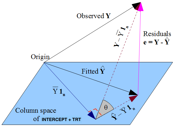
Figure 1: In the regression $\mathbb{E}[Y|A]$ of $Y$ on $A$ (the treatment variable), the fitted $\hat{\bm{Y}}$ is the orthogonal projection of the observed $\bm{Y}$ onto the column space spanned by the treatment $A$ and the intercept “1” which is represented by the blue plane. The fitted vector for the “1” (i.e., the intercept)-only model $\mathbb{E}[Y]$ is represented by $\bar{Y}\bm{1}_{n}$. The magnitude of the interaction effect between $A$ and “1” is quantified by the squared length of the vector $\hat{\bm{Y}}-\bar{Y}\bm{1}_{n}$.

For illustration, we consider a very simple example of regressing $Y$ on the treatment variable $A\in\mathcal{A}$ with no covariate $\bm{X}$ (i.e., the $\bm{X}$ corresponds to the intercept “1”). In this simple setting, the solution $\{g_{a}^{\ast}\}_{a\in\mathcal{A}}$ in (5.1) are just constants:

$$g_{a}^{\ast}=\mathbb{E}[Y|A=a]-\mathbb{E}[Y]\quad(a\in\mathcal{A}).$$ (5.2)

Given sample data $(y_{i},a_{i})$ $(i=1,\ldots,n)$, let $\bm{Y}=(y_{1},\ldots,y_{n})^{\top}$ denote the (length-$n$) observed vector of responses. The second term $\mathbb{E}[Y]$ on the right-hand side of (5.2) is represented by the (length-$n$) vector $\bar{Y}\bm{1}_{n}$, in which $\bar{Y}=\sum_{i=1}^{n}y_{i}/n$ is the grand mean of $Y$, and $\bm{1}_{n}=(1,1,\ldots,1)^{\top}$. The first term $\mathbb{E}[Y|A=a]$ $(a\in\mathcal{A})$ on the right-hand side of (5.2) is represented by the (length-$n$) vector $\hat{\bm{Y}}=(\hat{Y}_{1},\ldots,\hat{Y}_{n})^{\top}$, where $\hat{Y}_{i}=\sum_{a=1}^{L}1_{(a_{i}=a)}\bar{Y}^{(a)}$ $(i=1,\ldots,n)$, with $\bar{Y}^{(a)}=\sum_{i=1}^{n}y_{i}1_{(a_{i}=a)}/\sum_{i=1}^{n}1_{(a_{i}=a)}$ denoting the treatment $a$-specific mean. The fitted function $g_{A}^{\ast}$ in (5.2) is thus represented (in $\mathbb{R}^{n}$) by the vector $\hat{\bm{Y}}-\bar{Y}\bm{1}_{n}$. These three vectors ($\bar{Y}\bm{1}_{n}$, $\hat{\bm{Y}}$ and $\hat{\bm{Y}}-\bar{Y}\bm{1}_{n}$) in $\mathbb{R}^{n}$ are represented in Figure 1.

By constraint in the second line of (4.1), $\mathbb{E}[g_{A}^{\ast}]=0$ and thus, $\mbox{var}[g_{A}^{\ast}]=\mathbb{E}[(g_{A}^{\ast})^{2}]$ which is represented by $\lVert\hat{\bm{Y}}-\bar{Y}\bm{1}_{n}\rVert^{2}$ in Figure 1. Notice that the fitted vector, $\hat{\bm{Y}}-\bar{Y}\bm{1}_{n}$, is orthogonal to the “nuisance” vector $\bar{Y}\bm{1}_{n}$ in Figure 1.

Intuitively, the “effect” of intercept “1” in the intercept-only model is to average the response $\bm{Y}$, which results in the fit $\bar{Y}\bm{1}_{n}$ in Figure 1. The variance $\lVert\hat{\bm{Y}}-\bar{Y}\bm{1}_{n}\rVert^{2}\sim\mbox{var}[g_{A}^{\ast}]$, where $\hat{\bm{Y}}$ is the vector of treatment $a$-specific averages, quantifies the magnitude of how much the “effect” of intercept “1” (i.e., the grand averaging) is modified by the variable $A$, and hence the variance $\lVert\hat{\bm{Y}}-\bar{Y}\bm{1}_{n}\rVert^{2}$ quantifies the intensity of the “interaction effect” between the intercept “1” and $A$. Analogously, in the optimization framework (4.1), given a candidate $\bm{\beta}\in\Theta_{1}$, the variance of the profile minimizer $\{g_{a}^{\ast}\}_{a\in\mathcal{A}}$ in (5.1), i.e., $\mbox{var}\left[g_{A}^{\ast}({\bm{\beta}}^{\top}\bm{X})\right]=\mathbb{E}\left[\{g_{A}^{\ast}({\bm{\beta}}^{\top}\bm{X})\}^{2}\right]$, quantifies the magnitude of the interaction effect between the candidate linear predictor (i.e., single-index) ${\bm{\beta}}^{\top}\bm{X}$ and the variable $A$. This variance of the interaction effect is to be maximized over $\bm{\beta}\in\Theta_{1}$, as in the case of maximizing the variance (3.7).

When ${\bm{\beta}}^{\top}\bm{X}$ replaces the intercept “1”, for each $\bm{\beta}\in\Theta_{1}$, the blue plane in Figure 1, represents the Hilbert space of measurable functions of $({\bm{\beta}}^{\top}\bm{X},A$). Maximizing the variance of the $\bm{X}$-by-$A$ interaction effect, i.e., $\mbox{var}\left[g_{A}^{\ast}({\bm{\beta}}^{\top}\bm{X})\right]$, over ${\bm{\beta}}\in\Theta_{1}$ corresponds to adjusting the blue plane of Figure 1, in such a way that the blue plane minimizes the angle $\theta$ formed by the hypotenuse $\bm{Y}-\bar{Y}\bm{1}_{n}$ and the adjacent $\hat{\bm{Y}}-\bar{Y}\bm{1}_{n}$ (i.e., the $\theta$ formed by the two dashed lines in Figure 1). Or equivalently, it corresponds to maximizing the cosine of the angle $\theta$ (over $\bm{\beta}\in\Theta_{1}$), thereby maximizing the length of the vector $\lVert\hat{\bm{Y}}-\bar{Y}\bm{1}_{n}\rVert^{2}$.

Finally, we note that the two centered vectors $\hat{\bm{Y}}-\bar{Y}\bm{1}_{n}$ and $\bm{Y}-\bar{Y}\bm{1}_{n}$ (i.e., the two dashed lines in Figure 1) correspond to the fitted ($\hat{\bm{Y}}$) and the observed ($\bm{Y}$) vectors, respectively, centered by the intercept vector $(\bar{Y}\bm{1}_{n})$. Without centering by the intercept $\bar{Y}\bm{1}_{n}$, there is no Pythagorean-type sum of squares decomposition:

$$\lVert\bm{Y}-\bar{Y}\bm{1}_{n}\rVert^{2}=\lVert\bm{Y}-\hat{\bm{Y}}\rVert^{2}+\lVert\hat{\bm{Y}}-\bar{Y}\bm{1}_{n}\rVert^{2},$$ (5.3)

in which the second term, $\lVert\hat{\bm{Y}}-\bar{Y}\bm{1}_{n}\rVert^{2}$, quantifies the $A$-by-“$1$” interaction effect. Analogously, the “shifting” component $-\mathbb{E}[Y|{\bm{\beta}}^{\top}\bm{X}]$ in (5.1) plays the role of an “intercept.” Centering by the function $\mathbb{E}[Y|{\bm{\beta}}^{\top}\bm{X}]$ allows the following Pythagorean-type decomposition and isolates the variance associated with the interaction effect:

$$\mathbb{E}\big{[}\big{(}Y-\mathbb{E}[Y|{\bm{\beta}}^{\top}\bm{X}]\big{)}^{2}\big{]}=\mathbb{E}\big{[}\big{(}Y-\mathbb{E}[Y|{\bm{\beta}}^{\top}\bm{X},A]\big{)}^{2}\big{]}+\mathbb{E}\big{[}\big{(}\mathbb{E}[Y|{\bm{\beta}}^{\top}\bm{X},A]-\mathbb{E}[Y|{\bm{\beta}}^{\top}\bm{X}]\big{)}^{2}\big{]},$$ (5.4)

where the magnitude of the $A$-by-${\bm{\beta}}^{\top}\bm{X}$ interaction effect is quantified by the second term $\mathbb{E}\big{[}\big{(}g_{A}^{\ast}({\bm{\beta}}^{\top}\bm{X})\big{)}^{2}\big{]}=\mathbb{E}\big{[}\big{(}\mathbb{E}[Y|{\bm{\beta}}^{\top}\bm{X},A]-\mathbb{E}[Y|{\bm{\beta}}^{\top}\bm{X}]\big{)}^{2}\big{]}$ (see (5.1), for this equality), that is to be maximized over ${\bm{\beta}}\in\Theta_{1}$.

6 SUFFICIENT REDUCTION FOR INTERACTIONS BETWEEN COVARIATES AND A CONTINUOUS VARIABLE

In this section, we extend the semiparametric dimension reduction model to the case where the variable $A$ is defined on a compact continuum $\mathcal{A}\subset\mathbb{R}$. In this case, we can define a contrast function $\bm{c}\in\{\bm{c}:0<\int_{\mathcal{A}}{\bm{c}}^{2}(a)da,\int_{\mathcal{A}}{\bm{c}}(a)da=0\}\subset L^{2}(\mathcal{A})$, and the associated mean contrast function $\mathcal{C}(\bm{X};{\bm{c}}):=\int_{\mathcal{A}}\bm{c}(a)\mathbb{E}\left[Y|\bm{X},A=a\right]da$. We consider the dimension reduction model of form

$$\mathbb{E}\left[Y\mid\bm{X},A\right]=\mu(\bm{X})+g_{0}\big{(}\bm{B}_{0}^{\top}\bm{X},A\big{)},$$ (6.1)

where the smooth function $g_{0}$ is a ($q+1$ dimensional) function of $(\bm{B}_{0}^{\top}\bm{X},A)$, with the resulting function $g_{0}(\bm{B}_{0}^{\top}\bm{X},A)$ determining the $\bm{X}$-by-$A$ interaction effect; the term $\mu(\bm{X})$ represents an unspecified main effect of $\bm{X}$. As in (2.6), we assume $\mathbb{E}[g_{0}\big{(}\bm{B}_{0}^{\top}\bm{X},A\big{)}|\bm{X}]=0$ and $\bm{B}_{0}\in\Theta_{q}$, for model identifiability. Let $\mathcal{H}_{q+1}^{(\bm{B})}$ denote the Hilbert space of measurable functions of $(\bm{B}^{\top}\bm{X},A)$ given each $\bm{B}\in\Theta_{q}$, and in model (6.1), we assume $g_{0}\in\mathcal{H}_{q+1}^{(\bm{B}_{0})}$.

As in Section 4, we focus on a rank-1 (i.e., $q=1$) approximation model with a vector $\bm{\beta}\in\Theta_{1}$. For a continuous $A\in\mathcal{A}$, we modify the optimization framework (4.1) that utilizes a set of treatment $a$-specific 1-D smooths $\{g_{a}\in\mathcal{H}^{(\bm{\beta})}\}_{a\in\mathcal{A}}$ to that with a single $2$-D smooth $g\in\mathcal{H}_{2}^{(\bm{\beta})}$:

$$(\hat{g},\hat{\beta})\quad= \underset{g\in\mathcal{H}_{2}^{(\bm{\beta})},\bm{\beta}\in\Theta_{1}}{\text{argmin}} E\big{[}\big{(}Y-g\big{(}\bm{\beta}^{\top}\bm{X},A)\big{)}^{2}\big{]}$$ (6.2)

subject to $$\mathbb{E}\left[g(\bm{\beta}^{\top}\bm{X},A)|\bm{\beta}^{\top}\bm{X}\right]=0$$

We briefly sketch below an iterative procedure to solve (6.2). As in Section 4, we can alternate between estimation of $\bm{\beta}\in\Theta_{1}$ and $g\in\mathcal{H}_{2}^{(\bm{\beta})}$. Again, the constraint in (6.2) can be absorbed into a (tensor-product) basis representation of the 2-D smooth $g$ by reparametrization.

Denoting $\eta=\bm{\beta}^{\top}\bm{X}$, (although other linear smoothers can also be utilized), let us focus on tensor products of $B$-splines (de Boor, 2001) to represent the smooth $g(\eta,A)$ in (6.2) for each fixed $\bm{\beta}$, with a set of separate difference penalties applied to the coefficients of the basis along the $\eta$ and $A$ axes, i.e., the tensor-product P-splines (Eilers and Marx, 2003). We shall use the tensor product of $2$ univariate cubic $B$-splines, say $\Psi$ and $\check{\Psi}$, with $d$ and $\check{d}$ equally-spaced $B$-spline basis functions placed along the $\eta$ and $A$ axes respectively. Associated with the $d$ and $\check{d}$-dimensional marginal bases are $d\times d$ and $\check{d}\times\check{d}$ roughness penalty matrices, which we write as $S$ and $\check{S}$ respectively.

For fixed $\eta_{i}=\bm{\beta}^{\top}\bm{x}_{i}$ $(i=1,\ldots,n)$, let us write the $n\times d$ (and $n\times\check{d}$) $B$-spline design matrix $\bm{\Psi}$ (and $\check{\bm{\Psi}}$), in which its $i$th row is $\bm{\Psi}_{i}=\Psi(\eta_{i})^{\top}$ (and $\check{\bm{\Psi}}_{i}=\check{\Psi}(a_{i})^{\top}$). Then, for each fixed $\bm{\beta}$, a flexible surface $g$ in (6.2) can be approximated at the points $(\eta_{i},a_{i})$ $(i=1,\ldots,n)$ (Marx, 2015),

$$\mbox{vec}\big{\{}g(\eta_{i},a_{i})\big{\}}=g(\eta_{n\times 1},a_{n\times 1})=\bm{D}\bm{\theta},$$ (6.3)

with the $n\times d\check{d}$ tensor product model matrix

$$\bm{D}=\left(\bm{\Psi}\otimes\bm{1}_{\check{d}}^{\top}\right)\odot\left(\bm{1}_{d}^{\top}\otimes\check{\bm{\Psi}}\right),$$ (6.4)

where $\odot$ denotes element-wise multiplication of matrices and $\bm{\theta}\in\mathbb{R}^{d\check{d}}$ is an unknown coefficient vector associated with the function $g$.

Wood (2006) noted that constructing tensor products of the form (6.3) is a general approach to producing tensor product smooths of several variables, constructed from the univariate (marginal) bases $\bm{\Psi}$ and $\check{\bm{\Psi}}$ separately, and can be utilized for a general $q>2$ case. Similarly, the roughness penalty matrices associated with the tensor product model (6.3) can be constructed from the individual roughness penalty matrices, $S$ and $\check{S}$, and are given by $\bm{S}=S\otimes\bm{I}_{\check{d}}$ and $\check{\bm{S}}=\bm{I}_{d}\otimes\check{S}$, for the axis directions $\eta$ and $A$, respectively; here, $\bm{I}$ denotes the identity matrix, and both $\bm{S}$ and $\check{\bm{S}}$ are square matrices of dimension $d\check{d}$.

We now impose the constraint in (6.2) on the smooth $g$ under the tensor product representation (6.3). For each fixed $\bm{\beta}$, the constraint in (6.2) on $g$ amounts to excluding the main effect of $\eta=\bm{\beta}^{\top}\bm{X}$ from the smooth $g$. We deal with this by reparametrizing the representation (6.3). Consider the following sum-to-zero (over the observed values) constraint for the marginal basis of $A$:

$$\bm{1}^{\top}\check{\bm{\Psi}}\check{\bm{\gamma}}=0,$$ (6.5)

for any $\check{\bm{\gamma}}\in\mathbb{R}^{\check{d}}$, where $\bm{1}$ is a length-$n$ vector of 1’s. With the constraint (6.5), the linear smoother associated with the basis $\check{\bm{\Psi}}$ cannot reproduce constant functions (Hastie and Tibshirani, 1999). That is, the linear constraint (6.5) removes the span of constant functions from the span of the marginal basis $\check{\bm{\Psi}}$, with the result that the tensor product basis, $\bm{D}$ in (6.3), will not include the main effect of $\eta$ that results from the product of the marginal basis $\bm{\Psi}$ (associated with $\eta$) with the constant function in the span of the other marginal basis $\check{\bm{\Psi}}$ (associated with $A$). Therefore, the resultant fit of the 2-D smooth $g$, under representation (6.3) subject to (6.5), excludes the main effect of $\eta$. See Section 5.6 of Wood (2017) for additional details. Incorporating such a linear constraint (6.5) on the model matrix $\bm{D}$ in (6.3) is given below.

The key is to find an (orthogonal) basis for the null space of the constraint (6.5), and then absorb the constraint into construction of $\bm{D}$ in (6.4). To be specific, we can create a $\check{d}\times(\check{d}-1)$ matrix $\bm{Z}$, such that if $\check{\bm{\gamma}}=\bm{Z}\check{\bm{\gamma}}^{\ast}$ for any $\check{\bm{\gamma}}^{\ast}\in\mathbb{R}^{\check{d}-1}$, then $\bm{1}^{\top}\check{\bm{\Psi}}\check{\bm{\gamma}}=0$, satisfying the constraint (6.5). Such a matrix $\bm{Z}$ can be found by a QR decomposition of $\check{\bm{\Psi}}^{\top}\bm{1}$. Then, we can reparametrize the marginal basis $\check{\bm{\Psi}}$ by $\check{\bm{\Psi}}^{\ast}\leftarrow\check{\bm{\Psi}}\bm{Z}$ (and the associated penalty matrix by $\check{S}^{\ast}\leftarrow\bm{Z}^{\top}\check{S}\bm{Z}$) and absorb the constraint (6.5) into its basis construction. Accordingly, the resulting reparametrized model matrix (6.4) is given by $\bm{D}^{\ast}\leftarrow\left(\bm{\Psi}\otimes\bm{1}_{\check{d}-1}^{\top}\right)\odot\left(\bm{1}_{d}^{\top}\otimes\check{\bm{\Psi}}^{\ast}\right)$ and the associated penalty matrices are $\bm{S}^{\ast}\leftarrow S\otimes\bm{I}_{\check{d}-1}$ and $\check{\bm{S}}^{\ast}\leftarrow\bm{I}_{d}\otimes\check{S}^{\ast}$, for the axis directions $\eta$ and $A$, respectively; $\bm{\theta}\in\mathbb{R}^{d\check{d}}$ in (6.3) is also reparametrized to $\bm{\theta}^{\ast}\in\mathbb{R}^{d(\check{d}-1)}$.

This sum-to-zero reparametrization enforcing (6.5) to representation (6.3) is simple, and creates a term $\mbox{vec}\big{\{}g(\eta_{i},a_{i})\big{\}}=\bm{D}^{\ast}\bm{\theta}^{\ast}$ that specifies such pure $\bm{X}$-by-$A$ interactions (plus the $A$ main effect) that are orthogonal to the $\bm{X}$ main effect. Provided that the orthogonality constraint issue is addressed, for each fixed $\bm{\beta}$, the criterion (6.2) can be represented by a penalized least squares criterion, $Q(\bm{\theta}^{\ast},\bm{\beta})=\lVert Y_{n\times 1}-\bm{D}^{\ast}\bm{\theta}^{\ast}\rVert^{2}+\lambda\bm{\theta}^{\ast\top}\bm{S}^{\ast}\bm{\theta}^{\ast}+\check{\lambda}\bm{\theta}^{\ast\top}\check{\bm{S}}^{\ast}\bm{\theta}^{\ast}$, in which the smoothing parameters $\lambda$ and $\check{\lambda}$ can be estimated by, for example, REML. Similar to Section 4, we can iterate between optimizing $\bm{\theta}^{\ast}$ and $\bm{\beta}$ until convergence.

7 MULTIPLE PROJECTIONS FOR SUFFICIENT REDUCTION

We have so far focused on single-dimensional approximations (i.e., $q=1$ case). In this section, we consider generalizations when a sufficient reduction for interactions requires $q>1$. Specifically, we consider a general case of solving (2.9) to approximate the $\bm{X}$-by-$A$ interaction effect term of model (2.6). Solving the right-hand side of (2.9) subject to $\bm{B}\in\Theta_{q}$ can be viewed as a manifold optimization over the space of $p\times q$ matrices subject to the constraint $\bm{B}^{\top}\bm{B}=\bm{I}_{q}$, a special case of the Stiefel manifold (see, e.g., Muirhead, 1982).

To solve such a constraint optimization problem on a manifold, in this paper, we employ R (R Development Core Team, 2019) package ManifoldOptim (Adragni et al., 2017) that wraps the C++ library ROPTLIB (Huang et al., 2016). Given a candidate matrix $\bm{B}=(\bm{\beta}_{1};\ldots;\bm{\beta}_{q})\in\Theta_{q}$, we can obtain an empirical version of the objective function on the right-hand side of (2.9), analogous to representation (4.6), as follows. For ease of illustration, let us focus on the $q=2$ case. For each candidate matrix $\bm{B}\in\Theta_{2}$, at given triplets $(\bm{\beta}_{1}^{\top}\bm{x}_{i},\bm{\beta}_{2}^{\top}\bm{x}_{i},a_{i})$ $(i=1,\ldots,n$) and two sets of marginal basis $\{\Psi_{r},r=1,\ldots,d\}$ and $\{\check{\Psi}_{s},s=1,\ldots,\check{d}\}$ associated with $\bm{\beta}_{1}^{\top}\bm{X}$ and $\bm{\beta}_{2}^{\top}\bm{X}$ respectively, the univariate (i.e., $q=1$) basis representation (4.3) can be extended to a $q(=2)$-dimensional tensor-product representation: $g_{a_{i}}(\bm{\beta}_{1}^{\top}\bm{x}_{i},\bm{\beta}_{2}^{\top}\bm{x}_{i})=\sum_{r=1}^{d}\sum_{s=1}^{\check{d}}\Psi_{r}(\bm{\beta}_{1}^{\top}\bm{x}_{i})\check{\Psi}_{s}(\bm{\beta}_{2}^{\top}\bm{x}_{i})\theta_{rs,a_{i}}=(\bm{\Psi}_{i}\otimes\check{\bm{\Psi}}_{i})\bm{\theta}_{a_{i}}$ $(i=1,\ldots,n)$ for some $a$-specific vectors $\bm{\theta}_{a}\in\mathbb{R}^{d\check{d}}$ $(a\in\mathcal{A})$. If the set $\mathcal{A}$ is a continuous set (as in Section 6), we can allow the coefficients $\bm{\theta}_{a}$ to vary smoothly over $a\in\mathcal{A}$, as is assumed in representation (6.3). This method of constructing a tensor-product model can be applied to a general $q>2$ case. Similarly, the associated model penalty matrices can be constructed from a set of $q$ roughness penalty matrices of the $q$ individual axes (as in Section 6). The linear constraint (4.4) (or, that of of type (6.5), if we work with a continuous set $\mathcal{A}$) can then be absorbed into the tensor product representation of the design and the associated penalty matrices. Thus, for each candidate $\bm{B}\in\Theta_{2}$, the penalized least squares criterion of the form (4.6) (with an appropriate change to the penalty term to penalize over the general $q$ number of axes) can be optimized over $\tilde{\bm{\theta}}$ (with the associated smoothing parameters estimated via, for example, REML), resulting in a profiled objective function over $\bm{B}\in\Theta_{2}$. To optimize over $\bm{B}\in\Theta_{q}$, we can utilize a quasi-Newton (e.g., BFGS; Fletcher, 1987) method based on numerical approximation to the gradient of the profiled objective function (with respect to $\bm{B}$) via finite differences, as implemented in ManifoldOptim (Adragni et al., 2017).

In practice, the structural dimension $q$ of the dimension reduction model (2.6) is unknown, and therefore it is viewed as a tuning parameter. We next describe how to choose the structural dimension $q$ from data. The solution $(g_{01},\ldots,g_{0L},\bm{B}_{0})$ on the left-hand side of (2.9) is optimal with respect to minimizing the Kullback-Leibler (K-L) divergence between the working model $\mathbb{E}[Y|\bm{X},A=a]\approx g_{a}(\bm{B}^{\top}\bm{X})$ $(g_{a}\in\mathcal{H}^{(\bm{B})},\bm{B}\in\Theta_{q})$ $(a=1,\ldots,L)$ subject to constraint $\mathbb{E}[g_{A}(\bm{B}^{\top}\bm{X})|\bm{X}]=0$ $(\forall\bm{B}\in\Theta_{q})$ and the true underlying model (2.6) (under Gaussian noise). We can utilize an estimate of the expected K-L divergence of the fitted working model given each value of $q$ based on a cross-validation, as a basis of model selection. Alternatively, we can utilize the Akaike information criterion (AIC; Akaike, 1974) based model selection, or the network information criterion (NIC) introduced by Murata and Amari (1994), a generalization of the AIC, in the context of artificial neural networks (ANN). For NIC, the number of hidden units corresponds to $q$ in our case. Davidson (2003) provides illustrations of the closeness between AIC and NIC, even when the candidate (i.e., the working) models are incorrectly specified. We have found that, AIC, as a simpler approximation to the (relative) expected K-L divergence than NIC, behaves closely to a cross-validation estimate of the expected K-L divergence, and is relatively straightforward to compute. In general, AIC is defined to be the negative log likelihood of the model, plus two times the (effective) number of parameters used in the model that penalizes the model complexity. In our setting, the smooths $\{g_{a}\}_{a\in\mathcal{A}}$ are represented by a finite dimensional basis $\Psi(\cdot)\in\mathbb{R}^{d}$ (for $q>1$, we use an appropriate tensor product representation) with the associated basis coefficients $\bm{\theta}_{a}$ penalized for the function smoothness. Therefore, to define the AIC penalty term, we utilize the effective degrees of freedom (Hastie and Tibshirani, 1999) associated with the basis coefficients $\bm{\theta}_{a}$, and also account for the smoothing parameter $(\lambda_{a})$ estimation uncertainty by the method of Wood et al. (2016), implemented through R package mgcv (Wood, 2019). Let $\mbox{AIC}_{q}^{(g)}$ denote AIC associated with the estimated smooths $g_{a}(\bm{B}^{\top}\bm{X})$ $(a\in\mathcal{A})$, for a fixed $\bm{B}\in\Theta_{q}$. Then, we add to $\mbox{AIC}_{q}^{(g)}$ the additional penalty term, $2q(p-1)$, associated with the $q(p-1)$ “free” parameters of the dimension reduction matrix $\bm{B}\in\Theta_{q}$, to define AIC of the model:

$$\mbox{AIC}_{q}^{(g)}+2q(p-1),$$ (7.1)

whch can be minimized (over $q$) to determine the structural dimension of model (2.6).

8 APPLICATION

In this section, we apply the concept of sufficient reduction to a dataset from a randomized clinical trial for treatment of major depressive depression, comparing three (i.e., $L=3$) treatment conditions $A=a$ $(a=1,2,3)$: $a=1$ corresponds to placebo; $a=2$ corresponds to fluoxetine-varying dose; $a=3$ corresponds to imipramine-varying dose. The outcome $Y$ is taken to be the improvement in depression symptom severity measured by the Hamilton rating scale for depression (HRSD), defined to be HRSD at week 0 - HRSD at week 8, and a larger value of $Y$ is desired. We consider $p=6$ pretreatment patient characteristics $\bm{X}=(X_{1},\ldots,X_{6})^{\top}$: baseline symptom severity ($X_{1}$) ranging from 1 (normal) to 7 (extremely ill); age ($X_{2}$); gender ($X_{3}$) (0 = female, 1 = male); height ($X_{4}$); weight ($X_{5}$); and days of current illness ($X_{6}$). Each variable is standardized to zero mean and unit variance. The number of subjects $n=369$.

First, we estimate the interaction effect part of the (1-D) linear $\bm{X}$-by-$A$ interaction effect model (3.4), optimized based on criterion (3.6). With $L=3$, there are at most two $(=L-1)$ nonzero eigenvalues associated with the ($6\times 6$) matrix $\bm{H}$ in (3.2). These two eigenvalues are $6.35$ and $0.31$, respectively. Compared to the first eigenvalue ($=6.35$, associated with $\bm{\xi}_{1}$), the second eigenvalue ($=0.31$, associated with $\bm{\xi}_{2}$) is relatively negligible. This indicates that the 1-D approximation model (3.4) with $\bm{\beta}=\bm{\xi}_{1}$ is essentially sufficient for modeling the $\bm{X}$-by-$A$ interaction effects, under the assumption that the linear interaction effect model (3.1) is correctly specified, and therefore, we do not consider a 2-D dimension reduction with the dimension reduction matrix $\bm{B}=(\bm{\xi}_{1};\bm{\xi}_{2})$ for this example. The estimated 1-D reduction vector is $\bm{\beta}_{1}=(0.24,0.13,-0.73,0.53,-0.08,0.30)^{\top}$, and the corresponding treatment $a$-specific $(a=1,2,3)$ linear model fits on the estimated reduction $\bm{\beta}_{1}^{\top}\bm{X}$ are illustrated in the left panel of Figure 2.

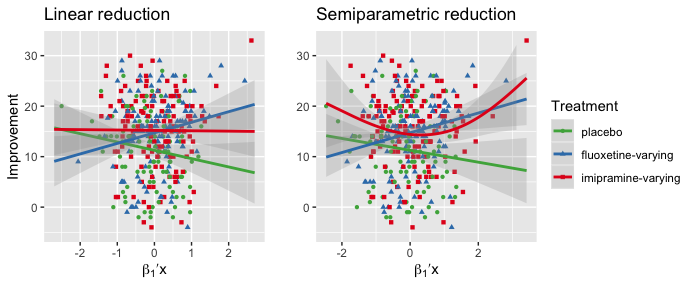
Figure 2: The scatter plots and the treatment $a$-specific functions $g_{a}(\cdot)$ ($a=1,2,3$; i.e., placebo, fluoxetine-varying dose and imipramine-varying dose, respectively) on the estimated 1-D reduction $\bm{\beta}_{1}^{\top}\bm{X}$, for the linear reduction (left) and the semiparametric reduction (right).

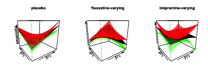
Figure 3: The treatment $a$-specific functions $g_{a}(\cdot)$ ($a=1,2,3$; i.e., placebo, fluoxetine-varying dose and imipramine-varying dose, respectively) on the estimated 2-dimensional reduction $(\bm{\beta}_{1}^{\top}\bm{X},\bm{\beta}_{2}^{\top}\bm{X})$; the red and green surfaces are at plus or minus one standard error from the estimated function (the black surface in the middle) conditional on the estimated $(\bm{\beta}_{1}^{\top}\bm{X},\bm{\beta}_{2}^{\top}\bm{X})$.

Second, we estimate the semiparametric dimension reduction model (2.6) with $q=1$ (i.e., 1-D reduction), optimized based on criterion (4.1). The estimated reduction vector is $\bm{\beta}_{1}=(0.42,0.26,-0.69,0.37,-0.14,0.34)^{\top}$, and the corresponding treatment $a$-specific ($a=1,2,3)$ curves on the estimated 1-D reduction $\bm{\beta}_{1}^{\top}\bm{X}$ are illustrated in the right panel of Figure 2. The “imipramine-varying dose” effect (i.e., $a=3)$ is clearly better captured by the flexible link function $g_{3}$ (the red curve) as compared to the linear reduction fit illustrated in the middle panel.

In addition, we estimate the semiparametric dimension reduction model (2.6) with $q=2$ (i.e., 2-D reduction), optimized based on criterion (2.9). The estimated reduction vectors are $\bm{\beta}_{1}=(0.56,0.10,-0.56,0.17,0.34,0.45)^{\top}$ and $\bm{\beta}_{2}=(0.29,-0.15,0.54,-0.32,-0.23,0.65)^{\top}$, and the corresponding treatment $a$-specific ($a=1,2,3)$ surfaces on the estimated 2-D reduction $(\bm{\beta}_{1}^{\top}\bm{X},\bm{\beta}_{2}^{\top}\bm{X})$ are illustrated in Figure 3.

To compare these three estimated dimension reduction models, we evaluate AIC (7.1). The resulting AIC values are $2529$, $2523$ and $2531$, for the 1-D linear, 1-D semiparametric, and 2-D semiparametric reduction models, respectively. The 1-D semiparametric reduction is favored, with respect to AIC (7.1). Lastly, since this dimension reduction framework for the $\bm{X}$-by-$A$ interaction effect was motivated from the problem of estimating the optimal individualized treatment rule $\mathcal{D}^{opt}$ in (2.3) that maximizes the value $V(\mathcal{D})$, we evaluate the performance of $\hat{\mathcal{D}}^{opt}$, with respect to the corresponding value $V(\hat{\mathcal{D}}^{opt})$, where $\hat{\mathcal{D}}^{opt}$ denotes an estimate of $\mathcal{D}^{opt}$ constructed based on each dimension reduction model. To estimate the value $V(\hat{\mathcal{D}}^{opt})$, we randomly split the dataset (of size $n=369$) at a ratio of $5$ to $1$ into a training set and a testing set (of size $\tilde{n}$), replicated $200$ times, each time computing $\hat{\mathcal{D}}^{opt}$ based on the training set and estimating the corresponding value $V(\hat{\mathcal{D}}^{opt})$ by an inverse probability weighted estimator (IPWE; Murphy, 2005): $\hat{V}(\hat{\mathcal{D}}^{opt})=\sum_{i=1}^{\tilde{n}}y_{i}1_{(a_{i}=\hat{\mathcal{D}}^{opt}(\bm{x}_{i}))}/\sum_{i=1}^{\tilde{n}}1_{(a_{i}=\hat{\mathcal{D}}^{opt}(\bm{x}_{i}))}$ evaluated based on the testing set. The resulting averages (and standard deviations) of $\hat{V}(\hat{\mathcal{D}}^{opt})$ over the 200 randomly split datasets are $14.72(1.32)$, $14.77(1.31)$ and $14.35(1.37)$, for the 1-D linear, 1-D semiparametric, and 2-D semiparametric reduction models, respectively. With respect to the value $V(\hat{\mathcal{D}}^{opt})$, the 1-D semiparametric reduction model is favored for this dataset.

9 DISCUSSION

Sufficient subspace reductions in regression of $Y$ on $(\bm{X},A)$ have typically been focused on the main effect of $(\bm{X},A)$. In some applications, such as precision medicine, with $A$ representing a treatment variable and $\bm{X}$ representing a set of pretreatment covariates, the primary concern is not on the main effect of $\bm{X}$ (which is often considered as a nuisance), but on the $\bm{X}$-by-$A$ interactions effect. In this paper, we extended the notion of sufficient subspace reduction for the $\bm{X}$ main effects to the $\bm{X}$-by-$A$ interaction effects in regression. We introduced a simple and easy-to-implement optimization framework to estimate a sufficient subspace for such an interaction effect. Linear model-based approaches (e.g., the modified covariate method) and the approach of using a single-index model to estimate the $\bm{X}$-by-$A$ interaction effects are connected in this optimization framework (2.9), in the context of a randomized clinical trial. This dimension reduction framework does not require to model the $\bm{X}$ main effects when reducing dimension for the $\bm{X}$-by-$A$ interaction effects. Although the results in Section 3 rely on the assumption that $A$ is distributed independently of $\bm{X}$, the general optimization framework (2.9) does not require such an assumption (see, e.g., the implementation of the semiparametric method in Sections 4). We also considered an extension of the methods to multiple projections of $\bm{X}$ and to the variable $A$ defined on a continuum.

One shortcoming of the dimension reduction framework presented in this paper is that the dimension reduction $R(\bm{X})=\bm{B}_{0}^{\top}\bm{X}$ for the $\bm{X}$-by-$A$ interactions is defined in terms of all the covariates $\bm{X}$ in the model, i.e., model (2.6) forces all the covariates play a role in building an interaction term. Also, estimating (2.6) in a high-dimensional $\bm{X}$ space is likely to cause problems of overfitting. Future work will employ an appropriate regularization for estimation of a sparse dimension reduction matrix $\bm{B}_{0}$ (subject to $\bm{B}_{0}\in\Theta_{q}$ for model identifiability), by utilizing, for example, a constrained $L^{1}$ regularization of Radchanko (2015) or a penalized approach of Peng and Huang (2011); Wang and Wang (2015), that can avoid overfitting as well as identify important covariates in $\bm{X}$ that modify the effects of $A$ on $Y$ as a result of the $\bm{X}$-by-$A$ interactions.

Supporting Information

Appendix:

The Appendix includes the proofs of Theorem 2.1, Corollary 2.1, Propositions 3.1, 3.2 and 3.4.

R-packages:

For the case of a 1-D (i.e., $q=1$) reduction, the R packages simml (Single-Index Models with Multiple-Links; Park et al., 2019a) developed for a categorical variable $A$ (described in Section 4) and simsl (Single-Index Models with a Surface-Link; Park et al., 2019b) developed for a continuous variable $A$ (described in Section 6), available on CRAN (R Development Core Team, 2019), provide an implementation of the proposed dimension reduction method.

Appendix A Appendix

Proof of Theorem 2.1

Proof.

Suppose there is a sufficient reduction $R(\bm{X})=\bm{B}_{0}^{\top}\bm{X}$ and the associated unspecified functions $\{g_{a}\}_{a\in\mathcal{A}}$, i.e., assume representation (2.5) (with $\bm{B}=\bm{B}_{0}$). Let $g_{0a}(\bm{B}_{0}^{\top}\bm{X})=g_{a}(\bm{B}_{0}^{\top}\bm{X})-\mathbb{E}[g_{A}(\bm{B}_{0}^{\top}\bm{X})|\bm{X}]$ $(a\in\mathcal{A})$, which, by rearrangement, gives $g_{a}(\bm{B}_{0}^{\top}\bm{X})=\mathbb{E}[g_{A}(\bm{B}_{0}^{\top}\bm{X})|\bm{X}]+g_{0a}(\bm{B}_{0}^{\top}\bm{X})$ $(a\in\mathcal{A})$, where, by definition, the term $\mathbb{E}[g_{A}(\bm{B}_{0}^{\top}\bm{X})|\bm{X}]$ does not depend on $a$ and the term $g_{0a}(\bm{B}_{0}^{\top}\bm{X})$ $(a\in\mathcal{A})$ satisfies (2.7). Thus, for any contrast vector $\bm{c}$, we can rewrite (2.5) (with $\bm{B}=\bm{B}_{0}$) as

$$\sum_{a=1}^{L}c_{a}g_{a}(\bm{B}_{0}^{\top}\bm{X})=\sum_{a=1}^{L}c_{a}\big{\{}\mathbb{E}[g_{A}(\bm{B}_{0}^{\top}\bm{X})|\bm{X}]+g_{0a}(\bm{B}_{0}^{\top}\bm{X})\big{\}}=\sum_{a=1}^{L}c_{a}g_{0a}(\bm{B}_{0}^{\top}\bm{X}),$$

where the second equality follows from $\sum_{a=1}^{L}c_{a}\mathbb{E}[g_{A}(\bm{B}_{0}^{\top}\bm{X})|\bm{X}]=\mathbb{E}[g_{A}(\bm{B}_{0}^{\top}\bm{X})|\bm{X}]\sum_{a=1}^{L}c_{a}=0$. Therefore, for representation (2.5), we can always reparametrize the set of functions $\{g_{a}\}_{a\in\mathcal{A}}$ by $\{g_{0a}\}_{a\in\mathcal{A}}$ that satisfies (2.7), implying that we can assume $g_{a}=g_{0a}$, without loss of generality. By definition (2.4), we can reexpress (2.5) (with $\bm{B}=\bm{B}_{0}$) as

$$\mathcal{C}(\bm{X};\bm{c})=\sum_{a=1}^{L}c_{a}\mathbb{E}\left[Y|\bm{X},A=a\right]=\sum_{a=1}^{L}c_{a}g_{0a}(\bm{B}_{0}^{\top}\bm{X}),$$ (A.1)

for any contrast vector $\bm{c}$. Under the general model (2.1), (A.1) indicates that the $\bm{X}$-by-$A$ interaction term $g(\bm{X},A=a)$ $(a\in\mathcal{A})$ in (2.1) corresponds to the term $g_{0a}(\bm{B}_{0}^{\top}\bm{X})$ $(a\in\mathcal{A})$ in (A.1), since (A.1) holds for an arbitrary contrast $\bm{c}=(c_{1},\ldots,c_{L})$. Furthermore, the term $\mu(\bm{X})$ in (2.1) corresponds to $\mu(\bm{X})$ of model (2.6), since $\mu(\bm{X})$ of model (2.6) represents the unspecified $\bm{X}$ marginal effect. Thus, under the general model (2.1), (2.5) implies model (2.6).

Conversely, if we assume model (2.6), then, by definition (2.4) we have

$$\mathcal{C}(\bm{X};\bm{c})\ =\ \sum_{a=1}^{L}c_{a}\mathbb{E}\left[Y|\bm{X},A=a\right]=\ 0\ +\ \sum_{a=1}^{L}c_{a}g_{0a}(\bm{B}_{0}^{\top}\bm{X}),$$ (A.2)

for all contrast vectors $\bm{c}$, where the $\bm{X}$ marginal effect $\mu(\bm{X})$ in (2.6) drops out due to $\sum_{a=1}^{L}c_{a}=0$. Expression (A.2) implies that $\bm{B}_{0}^{\top}\bm{X}$ is a sufficient reduction for $\mathcal{C}(\bm{X};\bm{c})$, implying (2.5) (with $\bm{B}=\bm{B}_{0}$). ∎

Proof of Corollary 2.1

Proof.

By Theorem 2.1, $R(\bm{X})=\bm{B}_{0}^{\top}\bm{X}$ of model (2.6) is a sufficient reduction (2.5). We need to show that $\mbox{span}(\bm{B}_{0})$ is a minimal reduction, and therefore $\mbox{span}(\bm{B}_{0})=S_{\mathcal{C}|\bm{X}}$. Due to the constraint (2.7), $\bm{B}_{0}$ of model (2.6) is not related to the $\bm{X}$ marginal effect, therefore there is no “nuisance” dimension contained in $\mbox{span}(\bm{B}_{0})$. Moreover, since $\bm{B}_{0}\in\Theta_{q}$, the columns of $\bm{B}_{0}$ are linearly independent. This implies $\bm{B}_{0}$ is a basis for $S_{\mathcal{C}|\bm{X}}$.

∎

Proof of Proposition 3.1

Proof.

Note that $\bm{\eta}_{a}-\bar{\bm{\eta}}\in\mbox{span}(\bm{\Xi})$ and hence $(\bm{\eta}_{a}-\bar{\bm{\eta}})^{\top}\bm{X}$ is measurable with respect to $\bm{X}^{\top}\bm{\Xi}$. If model (3.1) holds, then

$$\mathcal{C}\big{(}\bm{X}^{\top}\bm{\Xi};\bm{c}\big{)} = \sum_{a=1}^{L}{c_{a}E[Y\mid\bm{X}^{\top}\bm{\Xi},A=a]}$$

$$= \sum_{a=1}^{L}{c_{a}E[E[Y|\bm{X},A=a]\mid\bm{X}^{\top}\bm{\Xi},A=a]}$$

$$= \sum_{a=1}^{L}{c_{a}E[\tilde{\mu}(\bm{X})+\bm{\eta}_{a}^{\top}{\bm{X}\mid\bm{X}^{\top}\bm{\Xi},A=a]}}\;\;\mbox{by (\ref{linear.model})}$$

$$= \sum_{a=1}^{L}{c_{a}E[(\bm{\eta}_{a}-\bar{\bm{\eta}})^{\top}{\bm{X}\mid\bm{X}^{\top}\bm{\Xi},A=a]}}\;\;\mbox{(by zero-sum constraint on contrast $\bm{c}$)}$$

$$= \sum_{a=1}^{L}{c_{a}(\bm{\eta}_{a}-\bar{\bm{\eta}})^{\top}\bm{X}}\;\;\mbox{(by the measurability condition)}$$

$$= \sum_{a=1}^{L}{c_{a}(\tilde{\mu}(\bm{X})+\bm{\eta}_{a}^{\top}\bm{X})}\;\;\mbox{(by the zero-sum constraint on contrast $\bm{c}$)}$$

$$= \sum_{a=1}^{L}{c_{a}E[Y\mid\bm{X},A=a]}\;\;\mbox{(by (\ref{linear.model}))}$$

$$= \mathcal{C}\left(\bm{X};\bm{c}\right).$$

That $(\bm{\eta}_{1},\ldots,\bm{\eta}_{L})$ are distinct and $\pi_{a}>0$ is sufficient to guarantee that there are $L-1$ nonzero eigenvalues in the matrix $\bm{H}$ in (3.2). Since the “between” group dispersion matrix $\bm{H}$ in (3.2) has $L-1$ nonzero eigenvalues and the rank of $\bm{\Xi}$ is $L-1$, it is clear $\mbox{span}(\bm{\Xi})=S_{\mathcal{C}|\bm{X}}$.

∎

Proof of Proposition 3.2

Proof.

Let $Y_{a}$ denote $Y$ given $A=a$ $(a=1,\ldots,L)$, i.e., the $a$-specific outcome. For a given $\bm{\beta}$, consider the expression:

$$\mathbb{E}\left[(Y-\gamma_{A}{\bm{\beta}}^{\top}\bm{X})^{2}\right]=\sum_{a=1}^{L}\pi_{a}{\mathbb{E}\left[(Y_{a}-\gamma_{a}{\bm{\beta}}^{\top}\bm{X})^{2}1_{(A=a)}\right]}=\sum_{a=1}^{L}\pi_{a}{\mathbb{E}\left[(Y_{a}-\gamma_{a}{\bm{\beta}}^{\top}\bm{X})^{2}\right]},$$

which can be minimized by minimizing each of the $L$ terms with respect to $\gamma_{a}$ $(a=1,\dots,L)$ separately. For the uncentered $\tilde{\gamma}_{a}$, standard least-squares theory gives the solution as

$$\tilde{\gamma}_{a}={\mbox{cov}(\bm{\beta}^{\top}\bm{X},Y_{a})\over\mbox{var}(\bm{\beta}^{\top}\bm{X})}={\bm{\beta}^{\top}\mbox{cov}(\bm{X},Y_{a})\over\bm{\beta}^{\top}\bm{\Sigma}\bm{\beta}}\quad(a=1,\ldots,L).$$

Because $\bm{X}$ is centered and $Y_{a}$ is centered within each treatment $a$, the covariance in the numerator can be written as

$$\mbox{cov}(\bm{X},Y_{a})=\mathbb{E}[\bm{X}Y_{a}]=\mathbb{E}[\bm{X}\mathbb{E}[Y_{a}|\bm{X}]]=\mathbb{E}[\bm{X}\bm{X}^{\top}\bm{\eta}_{a}]=\mathbb{E}[\bm{X}\bm{X}^{\top}]\bm{\eta}_{a}=\bm{\Sigma}\bm{\eta}_{a},$$

and hence

$$\tilde{\gamma}_{a}={\bm{\beta}^{\top}\bm{\Sigma}\bm{\eta}_{a}\over\bm{\beta}^{\top}\bm{\Sigma}\bm{\beta}}\quad(a=1,\ldots,L).$$

Centering the $\tilde{\gamma}_{a}$ finishes the proof.

∎

Proof of Proposition 3.4

Proof.

Consider the criterion of (3.6) at the minimum:

$$(\ast\ast) =\min_{(\gamma_{1},\gamma_{2},\bm{\beta})}\ \mathbb{E}[(Y-\bm{X}^{\top}\bm{\beta}\gamma_{A})^{2}]$$ (A.3)

$$=\min_{(\gamma_{1},\gamma_{2},\bm{\beta})}\ \pi_{1}\mathbb{E}[(Y-\bm{X}^{\top}\bm{\beta}\gamma_{1})^{2}\mid A=1]+(1-\pi_{1})\mathbb{E}[(Y-\bm{X}^{\top}\bm{\beta}\gamma_{2})^{2}\mid A=2]$$

By Theorem 3.3, the minimum $(\ast\ast)$ occurs at $\bm{\beta}=\bm{\xi}_{1}$ and $\gamma_{a}=({\bm{\xi}_{1}}^{\top}\bm{\Sigma}{\bm{\xi}_{1}})^{-1}{\bm{\xi}_{1}}^{\top}\bm{\Sigma}(\bm{\eta}_{a}-\bar{\bm{\eta}})=({\bm{\xi}_{1}}^{\top}\bm{\Sigma}\bm{\xi}_{1})^{-1}{\bm{\xi}_{1}}^{\top}\bm{\Sigma}\left(\bm{\eta}_{a}-\{\pi_{1}\bm{\eta}_{1}+(1-\pi_{1})\bm{\eta}_{2}\}\right)$ $(a=1,2)$, that is:

$$\gamma_{1} =({\bm{\xi}_{1}}^{\top}\bm{\Sigma}\bm{\xi}_{1})^{-1}{\bm{\xi}_{1}}^{\top}\bm{\Sigma}(\bm{\eta}_{2}-\bm{\eta}_{1})(\pi_{1}-1)=\lVert\bm{\eta}_{2}-\bm{\eta}_{1}\rVert(\pi_{1}-1)\quad\mbox{and}$$ (A.4)

$$\gamma_{2} =({\bm{\xi}_{1}}^{\top}\bm{\Sigma}\bm{\xi}_{1})^{-1}{\bm{\xi}_{1}}^{\top}\bm{\Sigma}(\bm{\eta}_{2}-\bm{\eta}_{1})\pi_{1}=\lVert\bm{\eta}_{2}-\bm{\eta}_{1}\rVert\pi_{1},$$

which follows from $\bm{\xi}_{1}=(\bm{\eta}_{2}-\bm{\eta}_{1})/\lVert\bm{\eta}_{2}-\bm{\eta}_{1}\rVert$. Plugging (A.4) and $\bm{\beta}(=\bm{\xi}_{1})=(\bm{\eta}_{2}-\bm{\eta}_{1})/\lVert\bm{\eta}_{2}-\bm{\eta}_{1}\rVert$ into the second line of (A.3) gives:

$$(\ast\ast)= \pi_{1}\mathbb{E}[(Y-\bm{X}^{\top}(\bm{\eta}_{2}-\bm{\eta}_{1})(\pi_{1}-1))^{2}\mid A=1]\ +\ (1-\pi_{1})\mathbb{E}[(Y-\bm{X}^{\top}(\bm{\eta}_{2}-\bm{\eta}_{1})\pi_{1})^{2}\mid A=2]$$ (A.5)

$$= \pi_{1}\mathbb{E}[(Y-\bm{X}^{\top}{\bm{\beta}}(\pi_{1}-1))^{2}\mid A=1]+(1-\pi_{1})\mathbb{E}[(Y-\bm{X}^{\top}{\bm{\beta}}\pi_{1})^{2}\mid A=2]$$

$$= \pi_{1}\mathbb{E}[(Y-\bm{X}^{\top}{\bm{\beta}}(A+\pi_{1}-2))^{2}\mid A=1]+(1-\pi_{1})\mathbb{E}[(Y-\bm{X}^{\top}{\bm{\beta}}(A+\pi_{1}-2))^{2}\mid A=2]$$

$$= \ \mathbb{E}[(Y-\bm{X}^{\top}{\bm{\beta}}(A+\pi_{1}-2))^{2}],$$

in which we set $\bm{\beta}=(\bm{\eta}_{2}-\bm{\eta}_{1})\in\mathbb{R}^{p}$. The last line of (A.5) is the least squares criterion on the right-hand side of (3.10) associated with ${\bm{\beta}}^{\ast}$ of model (3.8). Since the minimum $(\ast\ast)$ (A.3) is unique, it follows that ${\bm{\beta}}^{\ast}=(\bm{\eta}_{2}-\bm{\eta}_{1})$, which is proportional to $\bm{\xi}_{1}=(\bm{\eta}_{2}-\bm{\eta}_{1})/\lVert\bm{\eta}_{2}-\bm{\eta}_{1}\rVert$. ∎

References

- Adragni and Cook (2009) Adragni, K. P. and Cook, D. R. (2009). Sufficient dimension reduction and prediction in regression. Philosophical Transactions of the Royal Society 367:4385–4405.
- Adragni et al. (2017) Adragni, K. P., Martin, S., Raim, A., and Huang, W. (2017). ManifoldOptim: An R interface to the ’ROPTLIB’ library for Riemannian manifold optimization. R package version 0.1.4 .
- Akaike (1974) Akaike, H. (1974). A new look at the statistical model identification. IEEE Transactions on Automatirc Control 19:716–723.
- Bura and Cook (2001) Bura, E. and Cook, R. D. (2001). Estimating the structural dimension of regression via parametric inverse regression. Journal of Royal Statistical Society: Series B 63.
- Cai et al. (2011) Cai, T., Tian, L., Wong, P. H., and Wei, L. J. (2011). Analysis of randomized comparative clinical trial data for personalized treatment selections. Biostatistics 12:270–282.
- Cook (1998) Cook, D. R. (1998). Regression Graphics. Wiley, New York.
- Cook and Li (2002) Cook, D. R. and Li, B. (2002). Dimension reduction for conditional mean in regression. The Annals of Statistics 30:455–474.
- Cook (1994) Cook, R. D. (1994). On the interpretation of regression plots. Journal of the American Statistical Association 89:177–189.
- Cook (1996) Cook, R. D. (1996). Graphics for regressions with a binary response. Journal of the American Statistical Association 91:983–992.
- Cook (2007) Cook, R. D. (2007). Fisher lecture: Dimension reduction in regression. Statistical Science 22:1–26.
- Davidson (2003) Davidson, A. (2003). Statistical Models. Cambridge: Cambridge University Press.
- de Boor (2001) de Boor, C. (2001). A Practical Guide to Splines. Springer-Verlag, New York.
- Eilers and Marx (1996) Eilers, P. and Marx, B. (1996). Flexible smoothing with B-splines and penalties. Statistical Science 11:89–121.
- Eilers and Marx (2003) Eilers, P. and Marx, B. (2003). Multivariate calibration with temperature interaction using two-dimensional penalized signal regression. Chemometrics and Intellegence Laboratory Systems 66:159–174.
- Fisher (1922) Fisher, R. A. (1922). On the mathematical foundations of theoretical statistics. Philosophical Transactions of the Royal Society 222:309–368.
- Fletcher (1987) Fletcher, R. (1987). Practical Methods of Optimization. Chichester, New York: Wiley.
- Hastie and Tibshirani (1999) Hastie, T. and Tibshirani, R. (1999). Generalized Additive Models. Chapman & Hall Ltd.
- Huang et al. (2016) Huang, W., Absil, P., Gallivan, K. A., and Hand, P. (2016). ROPTLIB: an object-oriented C++ library for optimization on Riemannian manifolds. Technical Report FSU16-14, Florida State University .
- Jeng et al. (2018) Jeng, X., Lu, W., and Peng, H. (2018). High-dimensional inference for personalized treatment decision. Electronic Journal of Statistics 12:2074–2089.
- Li (1991) Li, K.-C. (1991). Sliced inverse regression for dimension reduction (with discussion). Journal of the American Statistical Association 86:316–342.
- Li (1992) Li, K.-C. (1992). On principal Hessian directions for data visualization and dimension reduction: Another application of Stein’s lemma. Journal of the American Statistical Association 87:1025–1039.
- Lu et al. (2011) Lu, W., Zhang, H., and Zeng, D. (2011). Variable selection for optimal treatment decision. Statistical Methods in Medical Research 22:493–504.
- Luo et al. (2018) Luo, W., Wu, W., and Zhu, Y. (2018). Learning heterogeneity in causal inference using sufficient dimension reduction. Journal of Causal Inference 7.
- Luo et al. (2017) Luo, W., Zhu, Y., and Ghosh, D. (2017). On estimating regression-based causal effects using sufficient dimension reduction. Biometrika 104:51–65.
- Marx (2015) Marx, B. (2015). Varying-coefficient single-index signal regression. Chemometrics and Intellegence Laboratory Systems 143:111–121.
- Muirhead (1982) Muirhead, R. J. (1982). Aspects of Multivariate Statistical Theory. John Wiley & Sons, Inc., New York.
- Murata and Amari (1994) Murata, N. and Amari, S. (1994). Network Information Criterion- Determining the number of hidden units for an artificial neural network model. IEEE Transactions on Neural Networks 5:865–872.
- Murphy (2003) Murphy, S. A. (2003). Optimal dynamic treatment regimes. Journal of the Royal Statistical Society: Series B (Statistical Methodology) 65:331–355.
- Murphy (2005) Murphy, S. A. (2005). A generalization error for Q-learning. Journal of Machine Learning 6:1073–1097.
- Park et al. (2019a) Park, H., Petkova, E., Tarpey, T., and Ogden, R. (2019a). simml: single-index models with multiple-links. R package version 0.1.0 .
- Park et al. (2019b) Park, H., Petkova, E., Tarpey, T., and Ogden, R. (2019b). simsl: single-index models with a surface-link. R package version 0.1.0 .
- Park et al. (2020a) Park, H., Petkova, E., Tarpey, T., and Ogden, R. T. (2020a). A constrained single-index regression for estimating interactions between a treatment and covariates. Revision submitted to Biometrics .
- Park et al. (2020b) Park, H., Petkova, E., Tarpey, T., and Ogden, R. T. (2020b). A single-index model with multiple-links. Journal of Statistical Planning and Inference 205:115–128.
- Peng and Huang (2011) Peng, H. and Huang, T. (2011). Penalized least squares for single index models. Journal of Statistical Planning and Inference 141:1362–1379.
- Petkova et al. (2016) Petkova, E., Tarpey, T., Su, Z., and Ogden, R. T. (2016). Generated effect modifiers in randomized clinical trials. Biostatistics 18:105–118.
- Qian and Murphy (2011) Qian, M. and Murphy, S. A. (2011). Performance guarantees for individualized treatment rules. The Annals of Statistics 39:1180–1210.
- R Development Core Team (2019) R Development Core Team (2019). R: A Language and Environment for Statistical Computing. R Foundation for Statistical Computing, Vienna, Austria.
- Radchanko (2015) Radchanko, P. (2015). High dimensional single index model. Journal of Multivariate Analysis 139:266–282.
- Robins (2004) Robins, J. (2004). Optimal Structural Nested Models for Optimal Sequential Decisions. Springer, New York.
- Rubin (1974) Rubin, D. (1974). Estimating causal effects of treatments in randomized and nonrandomized studies. Journal of Educational Psychology 66:688–701.
- Shi et al. (2018) Shi, C., Fan, A., Song, R., and Lu, W. (2018). High-dimensional A-learning for optimal dynamic treatment regimes. The Annals of Statistics 46:925–957.
- Shi et al. (2016) Shi, C., Song, R., and Lu, W. (2016). Robust learning for optimal treatment decision with np-dimensionality. Electronic Journal of Statistics 10:2894–2921.
- Tian et al. (2014) Tian, L., Alizadeh, A., Gentles, A., and Tibshrani, R. (2014). A simple method for estimating interactions between a treatment and a large number of covariates. Journal of the American Statistical Association 109:1517–1532.
- Wang and Wang (2015) Wang, G. and Wang, L. (2015). Spline estimation and variable selection for single-index prediction models with diverging number of index parameters. Journal of Statistical Planning and Inference 162:1–19.
- Wood (2006) Wood, S. N. (2006). Low-rank scale-invariant tensor product smooths for generalized additive mixed models. Biometrics 62:1025–1036.
- Wood (2017) Wood, S. N. (2017). Generalized Additive Models: An Introduction with R. Chapman & Hall/CRC, second edition.
- Wood (2019) Wood, S. N. (2019). mgcv: Mixed GAM computation vehicle with automatic smoothness estimation. R package version 1.8.28 .
- Wood et al. (2016) Wood, S. N., Pya, N., and Safken, B. (2016). Smoothing parameter and model selection for general smooth models. Journal of the American Statistical Association 111:1548–1575.
- Yin et al. (2008) Yin, X., Li, B., and Cook, D. R. (2008). Successive direction extraction for estimating the central subspace in a multiple-index regression. Journal of Multivariate Analysis 99:1733–57.
- Zhang et al. (2012) Zhang, B., Tsiatis, A. A., Laber, E. B., and Davidian, M. (2012). A robust method for estimating optimal treatment regimes. Biometrics 68:1010–1018.