Fast Learning in Reproducing Kernel Kreĭn Spaces via Signed Measures

Abstract

In this paper, we attempt to solve a long-lasting open question for non-positive definite (non-PD) kernels in machine learning community: can a given non-PD kernel be decomposed into the difference of two PD kernels (termed as positive decomposition)? We cast this question as a distribution view by introducing the signed measure, which transforms positive decomposition to measure decomposition: a series of non-PD kernels can be associated with the linear combination of specific finite Borel measures. In this manner, our distribution-based framework provides a sufficient and necessary condition to answer this open question. Specifically, this solution is also computationally implementable in practice to scale non-PD kernels in large sample cases, which allows us to devise the first random features algorithm to obtain an unbiased estimator. Experimental results on several benchmark datasets verify the effectiveness of our algorithm over the existing methods.

1 Introduction

Devising a pairwise similarity/dissimilarity function plays a significant role in metric learning and kernel learning [28, 25, 62]. However, such function is not always positive definite (PD) in practice. For example, we are often faced with indefinite (real, symmetric, but not positive definite) kernels including the hyperbolic tangent kernel [54, 13] and truncated $\ell_{1}$-distance kernel [23]. Interestingly, some common-used PD kernels, e.g., polynomial kernels, Gaussian kernels, would degenerate to indefinite ones in some cases. An intuitive example is that a linear combination of PD kernels with negative coefficients [45]. Polynomial kernels using $\ell_{2}$-normalization (i.e., distributed on the unit sphere) are not always PD [46]. Gaussian kernels with some geodesic distances cannot be ensured positive definite [26, 21]. We refer to a survey [52] for details.

Learning with indefinite similarity/dissimilarity functions is typically modeled in Reproducing Kernel Kreĭn Spaces (RKKS) [44], where the (reproducing) indefinite kernel can be decomposed into the difference of two PD kernels, a.k.a, positive decomposition [9]. A series of work [49, 34, 42, 43, 50, 33] rely on the positive decomposition. It is important to note that, indefinite kernel matrices can be decomposed in the difference of two positive semi-definite matrices by eigenvalue decomposition, but for a given indefinite kernel, does it admit a positive decomposition? is a long-lasting open question in machine learning community. In fact, it appears non-trivial how to verify that an indefinite kernel can be associated with RKKS except for some intuitive examples, e.g., a linear combination of PD kernels with negative coefficients. In the past, we usually assume that a (reproducing) indefinite kernel is associated with RKKS in practice while the theoretical gap cannot be ignored. In particular, the used eigenvalue decomposition in indefinite kernel based algorithms [34, 42, 43] often incurs huge computational and space complexities and thus is infeasible to large-scale problems.

To answer the open question, we consider indefinite kernel in a distribution view. Our model is based on the signed measure, which generalizes Borel measure to be negative. Accordingly, the positive decomposition can be transformed to measure decomposition and thus we provide a sufficient and necessary condition to answer this question. Our distribution-based framework is simple but effective, which naturally allows us to devise unbiased random features based algorithm to scale indefinite kernel methods in large sample cases. Formally, we make the following contributions:

• In Section 3, by introducing the signed measure, we provide a sufficient and necessary condition to answer the above open question for indefinite kernels via the measure decomposition technique. Moreover, this condition also guides us how to find a specific positive decomposition in practice, and thus we can devise a unbiased estimator to obtain randomized feature maps. To the best of our knowledge, this is the first work to generate unbiased estimation for non-PD kernel approximation by random features.

• In Section 4, we demonstrate that spherically dot-product kernels including polynomial kernels, arc-cosine kernels, and the popular NTK in two-layer ReLU network on the unit sphere, are radial and non-PD associated with RKKS. Then we demonstrate the feasibility of our random feature algorithm on several indefinite kernels admitting the positive decomposition.

• In Section 5, we evaluate various non-PD kernels on several typical benchmark datasets to validate the effectiveness of our algorithm.

2 Preliminaries and Related Works

In this section, we briefly sketch some basic ideas of RKKS [9] and Bochner’s theorem in random features [48], and then introduce related works on indefinite kernel approximation.

2.1 Reproducing Kernel Kreĭn Spaces

Here we briefly review on the Kreĭn spaces and the reproducing kernel Kreĭn space (RKKS). Detailed expositions can be found in book [9]. Most of the readers would be familiar with Hilbert spaces. Kreĭn spaces share some properties of Hilbert spaces but differ in some key aspects which we shall emphasize as follows.

Kreĭn spaces are indefinite inner product spaces endowed with a Hilbertian topology.

Definition 2.1.

(Kreĭn space [9]) An inner product space is a Kreĭn space $\mathcal{H_{K}}$ if there exist two Hilbert spaces $\mathcal{H}_{+}$ and $\mathcal{H}_{-}$ such that
i) $\forall f\in\mathcal{H_{K}}$, it can be decomposed into $f=f_{+}\oplus f_{-}$, where $f_{+}\in\mathcal{H}_{+}$ and $f_{-}\in\mathcal{H}_{-}$, respectively.
ii) $\forall f,g\in\mathcal{H_{K}}$, $\langle f,g\rangle_{\mathcal{H_{K}}}=\langle f_{+},g_{+}\rangle_{\mathcal{H}_{+}}-\langle f_{-},g_{-}\rangle_{\mathcal{H}_{-}}$.

The Kreĭn space $\mathcal{H_{K}}$ can be decomposed into a direct sum $\mathcal{H_{K}}=\mathcal{H_{+}}\oplus\mathcal{H_{-}}$. Besides, the inner product on $\mathcal{H_{K}}$ is non-degenrate, i.e., for $f\in\mathcal{H_{K}}$, if $\langle f,g\rangle_{\mathcal{H_{K}}}=0$ for any $g\in\mathcal{H_{K}}$, we have $f=0$. From the definition, the decomposition $\mathcal{H_{K}}=\mathcal{H}_{+}\oplus\mathcal{H}_{-}$ is not necessarily unique. For a fixed decomposition, the inner product $\langle f,g\rangle_{\mathcal{H_{K}}}$ is given accordingly [34, 42]. The key difference from Hilbert spaces is that the inner products might be negative for Kreĭn spaces, i.e., there exists $f\in\mathcal{H_{K}}$ such that $\langle f,f\rangle_{\mathcal{H_{K}}}<0$. If $\mathcal{H}_{+}$ and $\mathcal{H}_{-}$ are two RKHSs, the Kreĭn space $\mathcal{H_{K}}$ is an RKKS associated with a unique indefinite reproducing kernel $k$ such that the reproducing property holds, i.e., $\forall f\in\mathcal{H_{K}},\leavevmode\nobreak\ f(x)=\langle f,k(x,\cdot)\rangle_{\mathcal{H_{K}}}$.

Proposition 2.1.

(positive decomposition [9]) Let $k:\mathbb{R}^{d}\times\mathbb{R}^{d}\rightarrow\mathbb{R}$ be a real-valued kernel function. Then there exists an associated RKKS identified with a reproducing kernel $k$ if and only if $k$ admits a positive decomposition $k=k_{+}-k_{-}$, where $k_{+}$ and $k_{-}$ are two positive definite kernels.

From the definition, this decomposition is not necessarily unique. As mentioned before, not every indefinite kernel function admits a representation as a difference between two positive definite kernels.

2.2 Bochner’s theorem and random features

A positive definite function corresponds to a nonnegative and finite Borel measure, i.e., a probability distribution, via Fourier transform by the following theorem.

Theorem 1 (Bochner’s Theorem [8]).

Let $k:\mathbb{R}^{d}\times\mathbb{R}^{d}\rightarrow\mathbb{R}$ be a bounded continuous function satisfying the stationary property, i.e., $k(\bm{x},\bm{x}^{\prime})=k(\bm{x}-\bm{x}^{\prime})$. Then, $k$ is positive definite if and only if it is the (conjugate) Fourier transform of a nonnegative and finite Borel measure $\mu$ (rescale it to a probability measure by setting $k(\bm{0})=1$)

$$k(\bm{x}-\bm{x}^{\prime})\!=\!\int_{\mathbb{R}^{d}}\!\!e^{\mathrm{i}{\bm{\omega}}^{\!\top}(\bm{x}-\bm{x}^{\prime})}\mu(\mathrm{d}{\bm{\omega}})=\mathbb{E}_{\bm{\omega}\sim\mu}\big{[}e^{\mathrm{i}{\bm{\omega}}^{\!\top}(\bm{x}-\bm{x}^{\prime})}\big{]}\,.$$

Typically, the kernel in practical uses is real-valued and thus the imaginary part can be discarded, i.e., $k(\bm{x}-\bm{x}^{\prime})=\mathbb{E}_{\bm{\omega}\sim\mu}\cos[\bm{\omega}^{\!\top}(\bm{x}-\bm{x}^{\prime})]$. Accordingly, we can use the Monte Carlo method to sample a series of random features $\{\bm{\omega}_{i}\}_{i=1}^{s}$ from the distribution $\mu$ to approximate the PD kernel function $k$, a.k.a. Random Fourier features (RFF) [48]. It brings promising performance and solid theoretical guarantees on scaling up kernel methods in classification [56], nonlinear component analysis [60, 35], and neural tangent kernel (NTK) [24]. Improvements on RFF mainly focus on variance reduction by advanced sampling methods, e.g., quasi-Monte Carlo sampling [61], Monte Carlo sampling with orthogonal constraints [64, 36, 17], leverage-score sampling [4, 29], and quadrature based methods [18, 41, 31], see a survey [30] for details.

2.3 Signed measure

Let $\mu:\mathcal{A}\rightarrow[0,+\infty]$ be a measure on a set $\Omega$ satisfying $\mu(\emptyset)=0$ and $\sigma$-additivity (i.e., countably additive). We call $\mu$ a finite measure if $\mu(\Omega)<+\infty$. Specifically, $\mu$ is a probability measure if $\mu(\Omega)=1$, and the triple $(\Omega,\mathcal{A},\mu)$ is referred as the corresponding probability space. Here we consider the signed measure, a generalized version of a measure allowing for negative values.

Definition 2.2.

(Signed measure [3]) Let $\Omega$ be some set, $\mathcal{A}$ be a $\sigma$-algebra of subsets on $\Omega$. A signed measure is a function $\mu:\mathcal{A}\rightarrow[-\infty,+\infty)\leavevmode\nobreak\ \mbox{or}\leavevmode\nobreak\ (-\infty,+\infty]$ satisfying $\sigma$-additivity.

Based on this definition, the following theorem shows that any signed measure can be represented by the difference of two nonnegative measures.

Theorem 2.

(Jordan decomposition [3]) Let $\mu$ be a signed measure defined on the $\sigma$-algebra $\mathcal{A}$ as given in Definition 2.2. There exists two (nonnegative) measures $\mu_{+}$ and $\mu_{-}$ (one of them is a finite measure) such that $\mu=\mu_{+}-\mu_{-}$.

The total mass of $\mu$ on $\mathcal{A}$ is defined as $\|\mu\|=\|\mu_{+}\|+\|\mu_{-}\|$. Note that this decomposition is not unique.

2.4 Related works

Learning with indefinite kernels in RKKS can be solved by eigenvalue transformation [11, 63], stabilization [44, 34], and minimization [42]. However, these methods need eigenvalue decomposition and cannot be directly applied to large-scale problems.

To scale indefinite kernel matrices in large sample problems, Nyström approximation works in a data-dependent way, and is a good choice to seek a low-rank representation to approximate indefinite kernel matrices, e.g., [43, 38, 51]. Besides, Liu et al. [32] decompose (a subset of) kernel matrix into two PD kernel matrices, and then learn their respective randomized feature maps by infinite Gaussian mixtures. However, this approach in fact focuses on approximating kernel matrices rather than kernel functions. If we consider indefinite kernel approximation by random features in a data-independent way, Pennington et al. [46] find that the polynomial kernel using $\ell_{2}$-normalized data is not PD, and then use (positive) mixtures of Gaussian distributions, associated with a PD kernel, to approximate it. This is in essence using a PD kernel to approximate an indefinite one. Till now, approximating non-PD kernels by random features cannot ensure unbiased and has not yet been fully investigated. In this paper, our work provides an unbiased estimator without extra parameters, so as to achieve both simplicity and effectiveness.

Besides, our algorithm can be also applied to dot-product kernels with $\ell_{2}$-normalized data, e.g., polynomial kernels on the unit sphere. Recent works for polynomial kernel approximation include Maclaurin expansion [27], the tensor sketch technique [47, 39], and oblivious subspace embedding [5, 59].

3 Model

In this section, by introducing the concept of signed measures [3], we attempt to answer the open question and then devise the sampling strategy for random features. For notational simplicity, we denote $z\coloneqq\|\bm{z}\|_{2}=\|\bm{x}-\bm{x}^{\prime}\|_{2}$ and $\omega\coloneqq\|\bm{\omega}\|_{2}$. Moreover, a function $k(\bm{z})$ is called radial if $k(\bm{z})=k(\|\bm{z}\|_{2})$. To notify, the considered stationary kernels in this paper are all radial, and their Fourier transforms are also radial, i.e., $\mu(\omega)=\mu(\bm{\omega})$, refer to [46, 10].

3.1 Answer to the open question in RKKS

As mentioned before, not every indefinite kernel admits a representation as a difference between two positive definite kernels. In fact we do not know how to verify that an indefinite kernel can be associated with RKKS except for some intuitive examples, e.g., a linear combination of PD kernels with negative coefficients. By virtue of measure decomposition of the signed measure in Theorem 2, we provide a sufficient and necessary condition in the following theorem to answer the question in RKKS: for a given indefinite kernel, does it admit a positive decomposition?

Theorem 3.

Assume that an indefinite kernel is stationary, i.e., $k(\bm{x},\bm{x}^{\prime})=k(\bm{x}-\bm{x}^{\prime})$. Denote its (generalized) Fourier transform as the measure $\mu$, then we have the following results:
(i) Existence: $k$ admits the positive decomposition, i.e., $k=k_{+}-k_{-}$, if and only if the total mass of the measure $\mu$ is finite, i.e., $\|\mu\|<\infty$. Here $k_{+}$ and $k_{-}$ are two reproducing kernels associated with two reproducing kernel Hilbert spaces (RKHS) $\mathcal{H}_{+}$ and $\mathcal{H}_{-}$, respectively.
(ii) Representation: If $\|\mu\|<\infty$, we choose $\mu_{+}$ and $\mu_{-}$ such that $\mu=\mu_{+}-\mu_{-}$, then the associated RKHSs $\mathcal{H}_{\pm}$ are given by

$$\mathcal{H}_{\pm}=\left\{f:\|f\|^{2}_{\mathcal{H}_{\pm}}=\int_{\mathbb{R}^{d}}\frac{|F(\bm{\omega})|^{2}}{\mu_{\pm}(\bm{\omega})}\mathrm{d}\bm{\omega}<\infty\right\}\,,$$

where $F(\bm{\omega})$ is the Fourier transform of $f$.

Proof    The proof can be found in Appendix A. ∎
Remark: We provide an explicit sufficient and necessary condition to link the Jordan decomposition of signed measures to positive decomposition in RKKS.
(i) Functions that can be written as a difference between two positive functions have been studied and characterized intrinsically in the field of harmonic analysis [37, 2, 1]. They partly answered this question either restricted in the one-dimensional case (i.e., $d=1$) or assuming the indefinite kernel $k(\bm{x},\bm{x}^{\prime})$ to be jointly analytic of $\bm{x}$ and $\bm{x}^{\prime}$ in a neighborhood of the origin. However, the used univariate condition could not be directly applied to the machine learning society and the smoothness requirement on kernels excludes some non-differentiable kernels, e.g., arc-cosine kernels. Instead, Theorem 3 provides an access via Fourier transform to verify whether a (reproducing) indefinite kernel belongs to RKKS or not. The measure decomposition is much easier to be founded than positive decomposition in RKKS that cannot be verified in practice.
(ii) Theorem 3 can be further improved to cover some non-squared-integrable kernel functions, e.g., conditionally positive definite kernels [58], of which the standard Fourier transform does not exist. In this case, Theorem 3 needs to consider the Fourier transform in Schwartz space [19]. For example, conditionally positive kernels correspond to a positive Borel measure $\mu$ on $\mathbb{R}^{d}\backslash\{\bm{0}\}$ with an analytic function in Schwartz space, refer to [55, Theorem 2.3].

3.2 Randomized feature map

$$\begin{split}k(\bm{x}-\bm{x}^{\prime})&=\!c_{1}\!\!\int_{\mathbb{R}^{d}}\!e^{\mathrm{i}{\bm{\omega}}^{\!\top}\!\bm{z}}\mu_{+}(\mathrm{d}{\bm{\omega}})\!-\!c_{2}\!\!\int_{\mathbb{R}^{d}}\!e^{\mathrm{i}{\bm{\nu}}^{\!\top}\!\bm{z}}\mu_{-}(\mathrm{d}{\bm{\nu}})=c_{1}\|\mu_{+}\|\mathbb{E}_{\bm{\omega}\sim\tilde{\mu}_{+}}\big{[}\cos(\bm{\omega}^{\!\top}\bm{z})\big{]}-c_{2}\|\mu_{-}\|\mathbb{E}_{\bm{\nu}\sim\tilde{\mu}_{-}}\big{[}\cos(\bm{\nu}^{\!\top}\bm{z})\big{]}\\ &\coloneqq k_{+}(\bm{x}-\bm{x}^{\prime})-k_{-}(\bm{x}-\bm{x}^{\prime})\approx\tilde{k}_{+}(\bm{x}-\bm{x}^{\prime})-\tilde{k}_{-}(\bm{x}-\bm{x}^{\prime})\\ &=\frac{1}{s}\sum_{i=1}^{s}\langle\mbox{Re}[\varphi_{i}(\bm{x})],\mbox{Re}[\varphi_{i}(\bm{x}^{\prime})]\rangle-\frac{1}{s}\sum_{i=1}^{s}\langle\mbox{Im}[\varphi_{i}(\bm{x})],\mbox{Im}[\varphi_{i}(\bm{x}^{\prime})]\rangle\,.\end{split}$$ (3.1)

The condition in Theorem 3 serves as a guidance for us to find a specific positive decomposition in practice. Hence we are ready to develop our random feature algorithm for (real-valued) non-PD kernels. One intuitive implementation way is choosing $\mu_{+}:=\max\{\mu,0\}$ and $\mu_{-}:=\min\{0,\mu\}$ such that $\mu=\mu_{+}-\mu_{-}$. Then the stationary indefinite kernel $k$ can be expressed by Eq. (3.1) via $k=k_{+}-k_{-}$ with two positive constants $c_{1}$, $c_{2}$. The decomposed two Borel measures $\tilde{\mu}_{+}\coloneqq\mu_{+}/\|\mu_{+}\|,\leavevmode\nobreak\ \tilde{\mu}_{-}\coloneqq\mu_{-}/\|\mu_{-}\|$ are associated with two (normalized) PD kernels $k_{+}$ and $k_{-}$, respectively. Accordingly, the stationary indefinite kernel $k$ can be approximated by $k\approx\tilde{k}:=\tilde{k}_{+}-\tilde{k}_{-}$. That is, $k(\bm{x},\bm{x}^{\prime})=\mathbb{E}_{\bm{\omega},\bm{\nu}}\left\langle\Phi(\bm{x}),\Phi(\bm{x}^{\prime})\right\rangle\!\approx\!\tilde{k}(\bm{x},\bm{x}^{\prime}):=\frac{1}{s}\!\sum_{i=1}^{s}\left\langle\varphi_{i}(\bm{x}),\varphi_{i}(\bm{x}^{\prime})\right\rangle$ where $\Phi(\bm{x})$ is the explicit feature mapping $\Phi(\bm{x})=[\varphi_{1}(\bm{x}),\cdots,\varphi_{s}(\bm{x})]^{\!\top}$ with $\varphi_{i}(\bm{x})$

$$\begin{split}&\varphi_{i}(\bm{x})\!=\!\!\Big{[}\sqrt{c_{1}\|\mu_{+}\|}\cos(\bm{\omega}_{i}^{\!\top}\bm{x}),\sqrt{c_{1}\|\mu_{+}\|}\sin(\bm{\omega}_{i}^{\!\top}\bm{x}),\quad\mathrm{i}\sqrt{c_{2}\|\mu_{-}\|}\!\cos(\bm{\nu}_{i}^{\!\top}\bm{x}),\mathrm{i}\sqrt{c_{2}\|\mu_{-}\|}\sin(\bm{\nu}_{i}^{\!\top}\bm{x})\Big{]}\,,\end{split}$$ (3.2)

where i is the imaginary unit. Then random features are obtained by sampling $\{\bm{\omega}_{i}\}_{i=1}^{s}\sim\mu_{+}/\|\mu_{+}\|$ and $\{\bm{\nu}_{i}\}_{i=1}^{s}\sim\mu_{-}/\|\mu_{-}\|$. The employed sampling method can be Monte Carlo sampling, orthogonal Monte Carlo sampling [64, 15], or leverage-score based sampling [4, 6]. The real and imaginary part in $\varphi_{i}(\bm{x})$ correspond to $k_{+}$ and $k_{-}$, and thus our estimation is unbiased. It is important to note that, we need the imaginary unit in the feature mapping due to the difference operation, and then the approximated kernel is still real-valued.

The complete random features process is summarized in Algorithm 1. For a given stationary indefinite kernel, its $\mu$, $\mu_{\pm}$ can be pre-computed, which is independent of the training data. In this way, our algorithm achieves the same complexity with the standard RFF by $\mathcal{O}(ns^{2})$ time and $\mathcal{O}(ns)$ memory. Besides, the formulation in Eq. (3.1), as well as Algorithm 1, is general enough to cover various PD and non-PD kernels. Stationary PD kernels admit Eq. (3.1) by choosing $c_{1}=1$ and $c_{2}=0$ where we have $\mu=\mu_{+}$ associated with $\|\mu\|=1$, i.e., a Borel measure. Hence, the Bochner’s theorem can be regarded as a special case of the considered integration representation (3.1) in this paper.

The approximation performance in our method for indefinite kernels still achieves theoretical guarantees with those of PD kernels by the following proposition. The result can be easily derived from [57, 16], of which the proof refers to Appendix B for completeness.

Proposition 3.1.

Let $k$ be a stationary indefinite kernel in RKKS with two Borel measures $\tilde{\mu}_{\pm}$ defined in Eq. (3.1), we have the following results:
(i) Approximation: Let $\mathcal{S}_{R}$ be the compact ball by $\mathcal{S}_{R}=\{\Delta|\Delta\in\mathbb{R}^{d},\|\Delta\|_{2}\leq R\}$, then given the approximated kernel $\tilde{k}$ obtained by our algorithm via Monte Carlo sampling, for any $\epsilon>0$

$$\operatorname{Pr}\!\left[\sup_{\bm{x},\bm{x}^{\prime}\in\mathcal{S}_{R}}\!|k(\bm{x},\bm{x}^{\prime})-\tilde{k}(\bm{x},\bm{x}^{\prime})|\geq\epsilon\right]\leq 66\left(\frac{2\sigma R}{\epsilon}\right)^{\!2}\!\!\!e^{-\frac{s\epsilon^{2}}{32(d+2)}},$$

where $\sigma^{2}:=\mathbb{E}_{\bm{\omega}\sim\tilde{\mu}_{+}}[{\bm{\omega}}^{\!\top}{\bm{\omega}}]+\mathbb{E}_{\bm{\omega}\sim\tilde{\mu}_{-}}[{\bm{\omega}}^{\!\top}{\bm{\omega}}]<\infty$.
(ii) Variance reduction: If we consider orthogonal Monte Carlo (OMC) sampling [64, 15] in our algorithm, it admits $\operatorname{MSE}[\tilde{k}^{\operatorname{OMC}}(\bm{x},\bm{x}^{\prime})]\leq\operatorname{MSE}[\tilde{k}^{\operatorname{MC}}(\bm{x},\bm{x}^{\prime})]$ for sufficiently large $d$, where the mean-squared error (MSE) is defined as $\mathbb{E}[\tilde{k}(\bm{x},\bm{x}^{\prime})]=\mathbb{E}[k(\bm{x},\bm{x}^{\prime})-\tilde{k}(\bm{x},\bm{x}^{\prime})]$.

Input: A kernel function $k(\bm{x},\bm{x}^{\prime})=k(z)$ with $z\coloneqq\|\bm{x}-\bm{x}^{\prime}\|_{2}$ and the number of random features $s$.

Output: Random feature map $\Phi(\cdot):\mathbb{R}^{d}\rightarrow\mathbb{R}^{4s}$ such that $k(\bm{x},\bm{x}^{\prime})\!\approx\!\frac{1}{s}\!\sum_{i=1}^{s}\left\langle\varphi_{i}(\bm{x}),\varphi_{i}(\bm{x}^{\prime})\right\rangle$.

1. Obtain the measure $\mu(\cdot)$ of the kernel $k$ via (generalized) Fourier transform ;

2. Given $\mu$, let $\mu\coloneqq\mu_{+}-\mu_{-}$ be the Jordan decomposition with two nonnegative measures $\mu_{\pm}$ and compute the total mass $\|\mu\|=\|\mu_{+}\|+\|\mu_{-}\|$;

3. Sample $\{\bm{\omega}_{i}\}_{i=1}^{s}\sim\mu_{+}/\|\mu_{+}\|$ and $\{\bm{\nu}_{i}\}_{i=1}^{s}\sim\mu_{-}/\|\mu_{-}\|$;

4. Output the explicit feature mapping $\Phi(\bm{x})$ with $\varphi_{i}(\bm{x})$ given in Eq. (3.2).

Algorithm 1 Random features for various indefinite kernels via generalized measures.

4 Examples

In this section, we investigate a series of indefinite kernels for a better understanding of our random features algorithm. We begin with an intuitive example, the linear combination of PD kernels with negative constraints. Then we discuss several dot-product kernels using $\ell_{2}$ normalization data, including the polynomial kernel [46], the arc-cosine kernel [14], and the NTK kernel in a two-layer ReLU network [7].

A linear combination of positive definite kernels with negative coefficients: Kernels in this class admit the formulation $k=\sum_{i=1}^{t}a_{i}k_{i}$, where $\{k_{i}\}_{i=1}^{t}$ is the set of PD kernels, and $a_{i}\in\mathbb{R}$. This is a typical example of indefinite kernels in RKKS, which admits positive decomposition such that $k=k_{+}-k_{-}$ with two PD kernels $k_{\pm}$. Theorem 3 guides us to find $\mu_{\pm}$ based on the sign of $a_{i}$. Hence we explicitly decompose an indefinite kernel in this class into the difference of two PD kernels, i.e., $k=k_{+}-k_{-}\coloneqq\sum_{i=1}^{t}\max(0,a_{i})k_{i}-\sum_{i=1}^{t}\max(0,-a_{i})k_{i}$. Then the corresponding nonnegative measures $\mu_{\pm}$ can be subsequently obtained due to the additivity of Fourier transform. We take the Delta-Gaussian kernel [42] $k(\bm{x},\bm{x}^{\prime})=\exp(-{\|\bm{x}-\bm{x}^{\prime}\|_{2}^{2}}/{2\tau_{1}^{2}})-\exp(-{\|\bm{x}-\bm{x}^{\prime}\|_{2}^{2}}/{2\tau_{2}^{2}})$ as an example. This kernel admits $c_{1}=c_{2}=1$ and $\|\mu_{+}\|=\|\mu_{-}\|=1$ in Eq. (3.1), and its random feature mapping is given by Eq. (3.2) with $\{\bm{\omega}_{i}\}_{i=1}^{s}\sim\mathcal{N}(0,\tau_{1}^{-2}\bm{I}_{d})$ and $\{\bm{\nu}_{i}\}_{i=1}^{s}\sim\mathcal{N}(0,\tau_{2}^{-2}\bm{I}_{d})$.

After providing the above simple warming-up example, we now discuss dot-product kernels on the unit sphere, and demonstrate the feasibility of our algorithm.

Polynomial kernels on the sphere: Pennington et al. [46] point out that a polynomial kernel on the unit sphere by $\ell_{2}$ normalization is of $k(\bm{x},\bm{x}^{\prime})=\left(1-\frac{\|\bm{x}-\bm{x}^{\prime}\|_{2}^{2}}{a^{2}}\right)^{p}$ for $a\geq 2$ and $p\geq 1$ and $z\coloneqq\|\bm{x}-\bm{x}^{\prime}\|_{2}\in[0,2]$. This kernel is indefinite since its Fourier transform is not a nonnegative measure in [46]

$$\mu(\omega)\!=\!\!\sum_{i=0}^{p}\frac{p!}{(p-i)!}\!\!\left(1\!-\!\frac{4}{a^{2}}\right)^{p-i}\!\!\left(\frac{2}{a^{2}}\right)^{i}\!\!\left(\frac{2}{\omega}\right)^{\frac{d}{2}+i}\!\!\!J_{\frac{d}{2}+i}(2\omega),$$ (4.1)

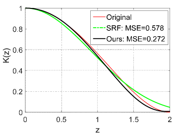
(a) graph of kernels

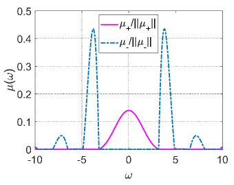
(b) signed measure $\mu$

Figure 1: Approximation of the spherical polynomial kernel with $a=p=2$.

which results from the oscillatory behavior of the Bessel function of the first kind $J_{d/2+i}(2\omega)$. We demonstrate $\|\mu\|<\infty$ (see in Appendix C), which makes the integration our random features algorithm feasible by decomposing $\mu=\mu_{+}-\mu_{-}$ with $\mu_{+}=\max\{0,\mu\}$ and $\mu_{-}=\min\{0,\mu\}$. Then random feature map for this kernel can be also given by Eq. (3.2) with $\{\bm{\omega}_{i}\}_{i=1}^{s}\sim\mu_{+}/\|\mu_{+}\|$ and $\{\bm{\nu}_{i}\}_{i=1}^{s}\sim\mu_{-}/\|\mu_{-}\|$. Therefore, Algorithm 1 is suitable for this kernel. Note that the (scaled) measure $\mu_{\pm}$ is not a typical probability distribution, but the radial property of the Fourier transform allows us to conduct rejection sampling in one dimension to sample from this “complex” distribution, which does not incur too much computational cost. We experimentally evaluate this with other sampling schemes in Section 5. Compared to [46] using a positive sum of Gaussians to approximate $\mu(\omega)$, where parameters in Gaussians need to be optimized aforehand, our algorithm achieves both simplicity and effectiveness by having (i) an unbiased estimator, (ii) incurring no extra parameters. Figure 1 shows the superiority of our method to SRF on approximating the spherical polynomial kernel $k(z)$. It can be found that, our method is unbiased to achieve lower mean squared error since SRF directly overlooks the negative part of the signed measure $\mu$.

Next we consider the NTK of two-layer ReLU networks on the unit sphere [7]. Since this kernel in fact consists of zero/first-order arc-cosine kernels [14], we combine them together for discussion.

NTK of Two-layer ReLU networks on the unit sphere: Bietti and Mairal [7] consider a two-layer ReLU network of the form $f(\bm{x};\bm{\theta})=\sqrt{2}{s}\sum_{j=1}^{s}\sum_{j=1}^{s}a_{j}\max\{\bm{\omega}_{j}^{\!\top}\bm{x},0\}$, with the parameter $\bm{\theta}=(\bm{\omega}_{1}^{\!\top},\cdots,\bm{\omega}_{s}^{\!\top},a_{1},\cdots,a_{s})$ initialized according to $\mathcal{N}(0,1)$. By formulating ReLU as $\max\{\bm{\omega}_{j}^{\!\top}\bm{x},0\}=(\bm{\omega}_{j}^{\!\top}\bm{x})_{+}$, we have the following formulation corresponding to NTK [7, 12]

$$k\left(\bm{x},\bm{x}^{\prime}\right)=2\mathbb{E}_{\bm{\omega}\sim\mathcal{N}(\bm{0},\bm{I})}\!\left[(\bm{\omega}^{\top}\!\bm{x})_{+}(\bm{\omega}^{\!\top}\!\bm{x}^{\prime})_{+}\right]$$ (4.2)

$$\!+\!2\left(\bm{x}^{\top}\!\bm{x}^{\prime}\right)\mathbb{E}_{\bm{\omega}\sim\mathcal{N}(\bm{0},\bm{I})}\!\left[1\left\{\bm{\omega}^{\top}\!\bm{x}\!\geq\!0\right\}\!1\!\left\{\bm{\omega}^{\top}\!\bm{x}^{\prime}\!\geq\!0\right\}\right],$$

which can be further represented by $k\left(\bm{x},\bm{x}^{\prime}\right)=\|\bm{x}\|\left\|\bm{x}^{\prime}\right\|\cdot\kappa\,\bigl{(}\left\langle\bm{x},\bm{x}^{\prime}\right\rangle/(\|\bm{x}\|\left\|\bm{x}^{\prime}\right\|)\!\bigr{)}$ with $\kappa(u)\coloneqq u\kappa_{0}(u)+\kappa_{1}(u)$. Here, $\kappa_{0}(u)=1-\frac{1}{\pi}\arccos(u)$ corresponds to the zero-order arc-cosine kernel and $\kappa_{1}(u)=\frac{1}{\pi}(u(\pi-\arccos(u))+\sqrt{1-u^{2}})$ is the first-order arc-cosine kernel [14]. Furthermore, such NTK kernel is proved to be stationary but indefinite by the following theorem.

Theorem 4.

For any $\bm{x},\bm{x}^{\prime}\in\mathbb{R}^{d}$, by $\ell_{2}$ normalization, the NTK kernel of a two layer ReLU network of the form $f(\bm{x};\bm{\theta})=\sqrt{2}{s}\sum_{j=1}^{s}\sum_{j=1}^{s}a_{j}\max\{\bm{\omega}_{j}^{\!\top}\bm{x},0\}$ is stationary, that is,

$$k(\bm{x},\bm{x}^{\prime})=\frac{2-z^{2}}{\pi}\arccos\left(\frac{1}{2}z^{2}-1\right)+\frac{z}{2\pi}\sqrt{4-z^{2}}\,,$$

where $z\coloneqq\|\bm{x}-\bm{x}^{\prime}\|_{2}\in[0,2]$. However, the function $k(z),z\in[0,2]$ is not positive definite.

Proof    The proof can be found in Appendix D. ∎
Since the above NTK on the unit sphere can be formulated as $k(\bm{x},\bm{x}^{\prime})=\langle\bm{x},\bm{x}^{\prime}\rangle\kappa_{0}(\bm{x},\bm{x}^{\prime})+\kappa_{1}(\bm{x},\bm{x}^{\prime})$ associated with arc-cosine kernels, we have the direct corollary for arc-cosine kernels.

Corollary 4.1.

The zero/first order arc-cosine kernel is not positive definite if the data are $\ell_{2}$-normalized, and its measure $\mu$ is given in Appendix E.

Remark: These spherical dot-product kernels including polynomial kernels, arc-cosine kernels, and NTK are indefinite by $\ell_{2}$ normalization, which extends the classical insight on spherical dot-product kernels via spherical harmonics [40]. Besides, our findings motivate us to scrutinize functional spaces, the approximation performance, and generalization properties of over-parameterized networks in deep learning theory if considering $\ell_{2}$-normalization data, which in return expands the usage scope of indefinite kernels.

In Appendix E, we compute the measure $\mu$ of arc-cosine kernels, which is quite complex as it involves with the sum of infinite series with Bessel functions. When taking finite series (e.g., one term) as an approximation, we demonstrate $\|\mu\|<\infty$. In this case, Algorithm 1 is accordingly suitable for arc-cosine kernels and NTK on the unit sphere. If we take more terms in finite series, the calculation appears non-trivial. And specifically, there exists a gap between the original $\mu$ and its approximation by finite series, so we do not include these two kernels in our experiments.

5 Experiments

We evaluate the proposed method on four representative benchmark datasets including letter, ijcnn1, covtype⁶, and cod-RNA⁶, see in Table 1. The datasets are normalized to $[0,1]^{d}$ by an $\ell_{2}$-norm scaling scheme and have been given with training/test partition except for covtype. Hence, we randomly split the covtype dataset into the training and test sets by half. In our experiment, the used indefinite kernels are the spherical polynomial kernel $k(\bm{x},\bm{x}^{\prime})=\left(1-{\|\bm{x}-\bm{x}^{\prime}\|_{2}^{2}}/{a^{2}}\right)^{p}$ with $a=2,\leavevmode\nobreak\ p=2$ in [46], and the Delta-Gaussian kernel $k(\bm{x},\bm{x}^{\prime})=\exp(-{\|\bm{x}-\bm{x}^{\prime}\|^{2}}/{2\tau_{1}^{2}})-\exp(-{\|\bm{x}-\bm{x}^{\prime}\|^{2}}/{2\tau_{2}^{2}})$ with $\tau_{1}=1$ and $\tau_{2}=10$ in [42]. The compared algorithms include SRF (Spherical Random Features) [46], DIGMM (Double-Infinite Gaussian Mixtures Model) [32], and Nyström with leverage score [43]. Moreover, we also include Random Maclaurin (RM) [27], Tensor Sketch (TS) [47], and Tensorized Random Projection (TRP) [39] for polynomial kernel approximation. Note that the related error bars and standard deviations are obtained by running the experiments for $10$ times. All experiments are implemented in MATLAB and carried out on a PC with Intel^® i7-8700K CPU (3.70 GHz) and 64 GB RAM. The source code of our implementation can be found in http://www.lfhsgre.org.

Table 1: Benchmark datasets.

Datasets	$d$	#training	#test
letter	16	12,000	6,000
ijcnn1	22	49,990	91,701
covtype	54	290,506	290,506
cod-RNA	8	59,535	157,413

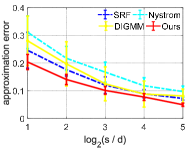
(a) letter

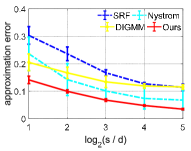
(b) ijcnn1

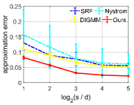
(c) covtype

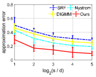
(d) cod-RNA

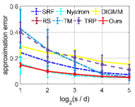
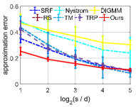
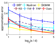
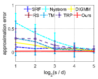
Figure 2: Comparisons of various algorithms for approximation error across the Delta-Gaussian kernel (top) and the spherical polynomial kernel (bottom) on four datasets.

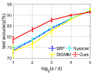
(a) letter

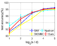
(b) ijcnn1

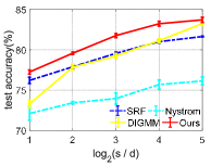
(c) covtype

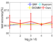
(d) cod-RNA

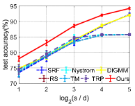
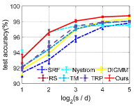
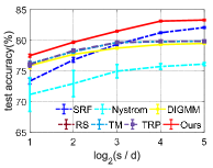
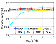
Figure 3: Comparisons of various algorithms for classification accuracy with LibLinear across the Delta-Gaussian kernel (top) and the spherical polynomial kernel (down) on four datasets.

Kernel approximation: The relative error $\|\bm{K}-\widetilde{\bm{K}}\|_{\mathrm{F}}/\|\bm{K}\|_{\mathrm{F}}$ is chosen to measure the approximation quality where $\bm{K}$ and $\widetilde{\bm{K}}$ denote the exact kernel matrix on 1,000 random selected samples and its approximated kernel matrix, respectively. Figure 2 shows the approximation error under two indefinite kernels as a function of #random features $s$. Our method achieves lower approximation error than the other algorithms across such two kernels on these datasets in most cases. A clear look at the case of Delta-Gaussian kernel approximation will find that our approach significantly improves the approximation quality compared to random features based algorithms: SRF and DIGMM. There always exists a gap in SRF that uses a PD kernel to approximate an indefinite one since the negative part is overlooked. DIGMM only focuses on approximating a subset of the kernel matrix. Different from these two, our method directly approximates the indefinite kernel function by an unbiased estimator, which incurs no extra loss for kernel approximation. Besides, when compared with several representative algorithms for polynomial kernels, e.g., RM, TS, and TRP, our method still performs well, which extends the application of our model.

Table 2: Time cost (sec.) for generating feature matrices of various algorithms.

Datasets	$s$	Spherical polynomial kernel							Delta-Gaussian kernel
		SRF1	Nyström	DIGMM	RM	TS	TRP	Ours	SRF1	Nyström	DIGMM	Ours
letter	$2d$	17.7+0.02	0.12	0.21	0.04	0.07	0.01	0.08	17.2+0.03	0.14	0.32	0.07
	$8d$	0.09	0.24	0.41	0.12	0.10	0.21	0.23	0.10	0.39	1.19	0.23
	$32d$	0.33	1.27	2.69	0.38	0.31	0.89	0.85	0.30	1.69	4.56	0.92
ijcnn1	$2d$	10.3+0.24	0.83	0.42	0.33	0.53	0.73	0.70	20.3+0.23	1.23	0.61	0.41
	$8d$	0.89	2.78	1.08	1.20	0.90	2.74	1.87	0.86	4.38	1.96	1.44
	$32d$	3.30	16.44	8.36	4.50	2.64	10.50	7.31	3.42	22.64	6.86	5.67

• On each dataset, SRF obtains parameters in GMM by an off-line grid search scheme in advance, of which this extra time cost is reported in bold.

Classification with linear SVM: We train a linear classifier: LibLinear [20] with the obtained randomized feature map. The balanced parameter in linear SVM is tuned by five-fold cross validation on a grid of points: $C=[0.01,0.1,1,10,100]$. The test accuracy of various algorithms are shown in Figure 3. As we expected, higher-dimensional randomized feature map outputs higher classification accuracy except the cod-RNA dataset. On this dataset, all of algorithms achieve the similar classification accuracy under various $s$. Apart from this dataset, our method performs best in most cases.

Computational time: Table 2 reports the time cost on generating randomized feature map with various dimensions $s$ on two datasets. Our method achieves the same complexity with the standard RFF with $\mathcal{O}(ns^{2})$ time and $\mathcal{O}(ns)$ memory. In practice, as reported by Table 2, our method takes a little more time than SRF to generate randomized feature maps due to the introduced extra imaginary part. Nevertheless, on each dataset, SRF requires extra time to obtain parameters of a sum of Gaussians in advance.

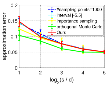
(a) approximation error

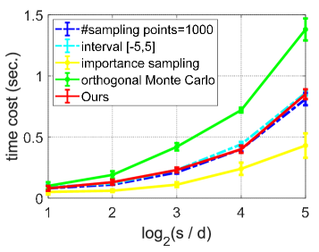
(b) time cost

Figure 4: Comparisons of various sampling schemes across the spherical polynomial kernel on letter.

Sampling schemes in spherical polynomial kernel: The measures $\mu_{+}/\|\mu_{+}\|$ and $\mu_{-}/\|\mu_{-}\|$ associated with the spherical polynomial kernel are not typical distributions, so we conduct rejection sampling to acquire them by generating a set of uniformly 10,000 samples in a range of $[-10,10]$. Here we compare various sampling schemes in our method for spherical polynomial kernel approximation, including sampling with 1,000 points, sampling in a sub-interval $[-5,5]$, importance sampling, and orthogonal Monte Carlo. Here the surrogate distribution in importance sampling is chosen as the Gaussian distribution. The applied orthogonal Monte Carlo, followed by [64], aims to obtain orthogonal random features.

Figure 4 shows the approximation error and time cost of various sampling schemes. It can be found that, orthogonal random features achieve lower approximation error but require more computational cost, as suggested by [64, 15]. Instead, the applied importance sampling decreases the time cost with a slight improvement on the approximation performance. If we choose the ridge leverage function in importance sampling, our model works with the leverage score based sampling, refer to [4] for details.

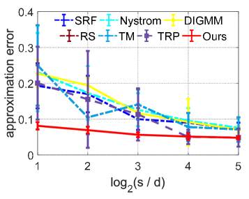
(a) order $p=1$

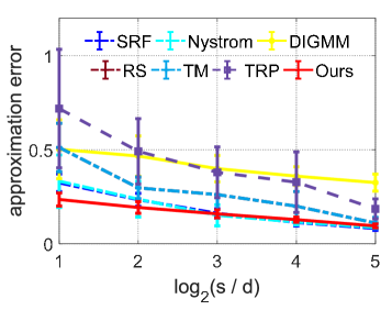
(b) order $p=3$

Figure 5: Approximation error of various algorithms across the spherical polynomial kernel with different orders on the letter dataset.

Different orders in spherical polynomial kernel: Apart from the used $p=2$ in the spherical polynomial kernel in our experiment, we evaluate our model on spherical polynomial kernels with various orders, e.g., $p=1$ and $p=3$. Kernel approximation results in Figure 5 show that, under different orders, our method performs better than other algorithms in terms of the approximation error.

6 Conclusion

We answer the open question of indefinite kernels in machine learning community by the introduced measure decomposition technique, which motivates us to develop a general random features algorithm across various kernels that are stationary indefinite kernels. Albeit simple, our algorithm is effective to output unbiased estimates for indefinite kernel approximation. Besides, our findings on the indefiniteness of NTK on the unit sphere (by $\ell_{2}$ normalization) encourages us to better understand the approximation performance, functional spaces, and generalization properties in over-parameterized networks in the future.

Appendix is organized as follows.

• Section A gives the proof of Theorem 3 on the studied open question.

• The approximation performance is theoretically demonstrated in Section B in terms of uniform approximation error bound and variance reduction.

• In Section (C), we demonstrate that polynomial kernels on the unit sphere by $\ell_{2}$ normalization data is with finite total mass.

• Section D gives the proof of Theorem 4.

• The measure of arc-cosine kernels on the unit sphere by $\ell_{2}$ normalization data is given in Section E.

Appendix A Proof of Theorem 3

Proof    We give the proof of the existence.
(i) Necessity.
An stationary indefinite kernel associated with RKKS admits the positive decomposition

$$k(\bm{x}-\bm{x}^{\prime})=k_{+}(\bm{x}-\bm{x}^{\prime})-k_{-}(\bm{x}-\bm{x}^{\prime})\,,\quad\forall\bm{x},\bm{x}^{\prime}\in X\,,$$

where $k_{+}$ and $k_{-}$ are two positive definite kernels. According to the Bochner’s theorem [8], there exists two probability measures $\mu_{+}$, $\mu_{-}$ such that

$$k(\bm{z})=k_{+}(\bm{z})-k_{-}(\bm{z})=\int_{\Omega}\exp\left(\mathrm{i}{\bm{\omega}}^{\!\top}\bm{z}\right)\mu_{+}(\mathrm{d}{\bm{\omega}})-\int_{\Omega}\exp\left(\mathrm{i}{\bm{\omega}}^{\!\top}\bm{z}\right)\mu_{-}(\mathrm{d}{\bm{\omega}})\,,$$

where $\bm{z}\coloneqq\bm{x}-\bm{x}^{\prime}$. Denote $\mu\coloneqq\mu_{+}-\mu_{-}$, it is clear that $\mu$ is a signed measure, and its total mass is finite because of $\|\mu\|=\|\mu_{+}\|+\|\mu_{-}\|=2$.

(ii) Sufficiency.
Let $\Omega\coloneqq\mathbb{R}^{d}$ and $\mathcal{A}$ be the smallest $\sigma$-algebra containing all open subsets of $\Omega$, and $\mu:\mathcal{A}\rightarrow[-\infty,\infty]$

$$\mu(\bm{\omega})=\int_{\Omega}\exp\left(-\mathrm{i}{\bm{\omega}}^{\!\top}\bm{z}\right)k(\bm{z})\mathrm{d}\bm{z}\,.$$

Since we assume that $\mu$ has total mass $\|\mu\|<\infty$, i.e., $\mu$ is finite, $\mu$ can be regarded as a signed measure. By virtue of Jordan decomposition in Theorem 2, there exist two nonnegative finite measures $\mu_{+}$ and $\mu_{-}$ such that $\mu=\mu_{+}-\mu_{-}$. One intuitive implementation way is choosing $\mu_{+}=\max\{\mu,0\}$ and $\mu_{-}=\min\{0,\mu\}$. Then using the inverse Fourier transform and Plancherel’s theorem [19], we have

$$\begin{split}k(\bm{z})=\int_{\Omega}\exp\left(\mathrm{i}{\bm{\omega}}^{\!\top}\bm{z}\right)\mu(\mathrm{d}{\bm{\omega}})&=\int_{\Omega}\exp\left(\mathrm{i}{\bm{\omega}}^{\!\top}\bm{z}\right)\mu_{+}(\mathrm{d}{\bm{\omega}})-\int_{\Omega}\exp\left(\mathrm{i}{\bm{\omega}}^{\!\top}\bm{z}\right)\mu_{-}(\mathrm{d}{\bm{\omega}})\\ &=\|\mu_{+}\|\int_{\Omega}\exp\left(\mathrm{i}{\bm{\omega}}^{\!\top}\bm{z}\right)\tilde{\mu}_{+}(\mathrm{d}{\bm{\omega}})-\|\mu_{-}\|\int_{\Omega}\exp\left(\mathrm{i}{\bm{\omega}}^{\!\top}\bm{z}\right)\tilde{\mu}_{-}(\mathrm{d}{\bm{\omega}})\\ &=\|\mu_{+}\|\tilde{k}_{+}(\bm{z})-\|\mu_{-}\|\tilde{k}_{-}(\bm{z})\,,\end{split}$$

where $\tilde{\mu}_{+}\coloneqq\mu_{+}/\|\mu_{+}\|$ and $\tilde{\mu}_{-}\coloneqq\mu_{-}/\|\mu_{-}\|$ are two nonnegative Borel measures, which correspond to two positive definite kernels $\tilde{k}_{+}$ and $\tilde{k}_{-}$, respectively. By defining $k_{+}\coloneqq\|\mu_{+}\|\tilde{k}_{+}$ and $k_{-}\coloneqq\|\mu_{+}\|\tilde{k}_{-}$, we have

$$k(\bm{x},\bm{x}^{\prime})=k_{+}(\bm{x},\bm{x}^{\prime})-k_{-}(\bm{x},\bm{x}^{\prime}),\quad\forall\bm{x},\bm{x}^{\prime}\in X\,.$$

This completes the proof.

Based on the above analysis, we give a characterization of the RKHSs $\mathcal{H}_{\pm}$ through the given spectral density $\mu_{\pm}$. In [22], a RKHS can be characterized by its measure via Fourier transform. Therefore, in our model, the RKHSs $\mathcal{H}_{\pm}$ are represented by $\mu_{\pm}$. That is, for any $f\in\mathcal{H}_{\pm}$, the inner product is induced by the Hilbert norm

$$\|f\|_{\mathcal{H}_{\pm}}^{2}=\int_{\mathbb{R}^{d}}\frac{|F(\bm{\omega})|^{2}}{\mu_{+}(\bm{\omega})}\mathrm{d}\bm{\omega}\,,$$

where $F(\bm{\omega})=\mathscr{F}(f)=\int_{\mathbb{R}^{d}}f(\bm{x})e^{-2\pi\mathrm{i}\bm{\omega}^{\!\top}\bm{x}}\mathrm{d}\bm{x}$ is the Fourier transform of $f$.

∎

Appendix B Proof of Proposition 3.1

The proof can be easily derived from [57, 16], and we briefly present here for completeness. Proof    Proposition 1 in [57] demonstrates

$$\operatorname{Pr}\!\left[\sup_{\bm{x},\bm{x}^{\prime}\in\mathcal{S}_{R}}\!|k_{\pm}(\bm{x},\bm{x}^{\prime})\!-\!\tilde{k}_{\pm}(\bm{x},\bm{x}^{\prime})|\geq\epsilon\right]\!\leq\!66\!\left(\frac{\sigma_{\pm}R}{\epsilon}\right)^{\!2}\exp\left(-\frac{s\epsilon^{2}}{8(d+2)}\right)\,,$$

where $\sigma_{\pm}^{2}=\mathbb{E}_{\bm{\omega}\sim\tilde{\mu}_{\pm}}[{\bm{\omega}}^{\!\top}{\bm{\omega}}]<\infty$. Since the indefinite kernel $k$ admits

$$|k(\bm{x},\bm{x}^{\prime})-\tilde{k}(\bm{x},\bm{x}^{\prime})|\leq|k_{+}(\bm{x},\bm{x}^{\prime})-\tilde{k}_{+}(\bm{x},\bm{x}^{\prime})|+|k_{-}(\bm{x},\bm{x}^{\prime})\!-\!\tilde{k}_{-}(\bm{x},\bm{x}^{\prime})|\,,\quad\forall\bm{x},\bm{x}^{\prime}\in\mathcal{S}_{R}\,,$$

then we have

$$\begin{split}\operatorname{Pr}\!\left[\sup_{\bm{x},\bm{x}^{\prime}\in\mathcal{S}_{R}}\!|k(\bm{x},\bm{x}^{\prime})\!-\!\tilde{k}(\bm{x},\bm{x}^{\prime})|\geq\epsilon\right]&\leq\operatorname{Pr}\!\left[\sup_{\bm{x},\bm{x}^{\prime}\in\mathcal{S}_{R}}\!|k_{+}(\bm{x},\bm{x}^{\prime})\!-\!\tilde{k}_{+}(\bm{x},\bm{x}^{\prime})|\geq\frac{\epsilon}{2}\right]+\operatorname{Pr}\!\left[\sup_{\bm{x},\bm{x}^{\prime}\in\mathcal{S}_{R}}\!|k_{-}(\bm{x},\bm{x}^{\prime})\!-\!\tilde{k}_{-}(\bm{x},\bm{x}^{\prime})|\geq\frac{\epsilon}{2}\right]\\ &\leq 66\!\left(\frac{2\sigma_{+}R}{\epsilon}\right)^{\!2}\exp\left(-\frac{s\epsilon^{2}}{32(d+2)}\right)+66\!\left(\frac{2\sigma_{-}R}{\epsilon}\right)^{\!2}\exp\left(-\frac{s\epsilon^{2}}{32(d+2)}\right)\\ &=66\!\left(\frac{2\sigma R}{\epsilon}\right)^{\!2}\exp\left(-\frac{s\epsilon^{2}}{32(d+2)}\right)\,.\end{split}$$

Then we study the variance reduction of the applied orthogonal Monte Carlo (OMC) sampling. Based on the definition of $\operatorname{MSE}$, i.e., $\mathbb{E}[\tilde{k}(\bm{x},\bm{x}^{\prime})]=\mathbb{E}[k(\bm{x},\bm{x}^{\prime})-\tilde{k}(\bm{x},\bm{x}^{\prime})]$, we conclude that $\mathbb{E}[\tilde{k}(\bm{x},\bm{x}^{\prime})]$ is the variance of $\tilde{k}(\bm{x},\bm{x}^{\prime})$, termed as $\operatorname{Var}[\tilde{k}(\bm{x},\bm{x}^{\prime})]$ due to our unbiased estimator. According to Theorem 4.2 in [16], for sufficiently large $d$, we have

$$\operatorname{MSE}[\tilde{k}_{+}^{\operatorname{OMC}}(\bm{x},\bm{x}^{\prime})]\leq\operatorname{MSE}[\tilde{k}_{+}^{\operatorname{MC}}(\bm{x},\bm{x}^{\prime})]\quad\mbox{and}\quad\operatorname{MSE}[\tilde{k}_{-}^{\operatorname{OMC}}(\bm{x},\bm{x}^{\prime})]\leq\operatorname{MSE}[\tilde{k}_{-}^{\operatorname{MC}}(\bm{x},\bm{x}^{\prime})]\,,$$

where $\bm{\omega}\sim\tilde{\mu}_{+}(\cdot)$ in $\tilde{k}_{+}$ and $\bm{\nu}\sim\tilde{\mu}_{-}(\cdot)$ in $\tilde{k}_{-}$ as indicated by Eq. (3.1). Since these two random vectors $\bm{\omega}$ and $\bm{\nu}$ are independent, we have

$$\operatorname{Var}[\tilde{k}^{\operatorname{OMC}}(\bm{x},\bm{x}^{\prime})]=\operatorname{Var}[\tilde{k}_{+}^{\operatorname{OMC}}(\bm{x},\bm{x}^{\prime})]+\operatorname{Var}[\tilde{k}_{-}^{\operatorname{OMC}}(\bm{x},\bm{x}^{\prime})]\leq\operatorname{Var}[\tilde{k}_{+}^{\operatorname{MC}}(\bm{x},\bm{x}^{\prime})]+\operatorname{Var}[\tilde{k}_{-}^{\operatorname{MC}}(\bm{x},\bm{x}^{\prime})]=\operatorname{Var}[\tilde{k}^{\operatorname{MC}}(\bm{x},\bm{x}^{\prime})]\,.$$

which implies $\operatorname{MSE}[\tilde{k}^{\operatorname{OMC}}(\bm{x},\bm{x}^{\prime})]\leq\operatorname{MSE}[\tilde{k}^{\operatorname{MC}}(\bm{x},\bm{x}^{\prime})]$ for sufficiently large $d$.

∎

Appendix C Polynomial kernels on the unit sphere with finite total mass

We consider the asymptotic properties of the Bessel function of the first kind $J_{\alpha}(x)$ under the large and small cases to study the $\|\mu\|$.

C.1 A small $\omega$

Consider the asymptotic behavior for small $\omega$. The Bessel function of the first kind is asymptotically equivalent to

$$J_{\alpha}(x)\sim\frac{1}{\Gamma(\alpha+1)}\left(\frac{x}{2}\right)^{\alpha}\,,\leavevmode\nobreak\ \mbox{when}\leavevmode\nobreak\ 0<x\ll\sqrt{\alpha+1}\,.$$

In this case, the measure $\mu$ is formulated as

$$\mu(\omega)\sim\sum_{i=0}^{p}\frac{p!}{(p-i)!}\left(1-\frac{4}{a^{2}}\right)^{p-i}\left(\frac{2}{a^{2}}\right)^{i}\frac{2^{d/2+i}}{\Gamma(d/2+i+1)}\,,$$ (C.1)

which can be regarded as a generalized version of a uniform distribution. Therefore, $\mu$ is absolutely integrable over a finite range $(0,c_{1}]$, where $c_{1}$ is some constant satisfying $c_{1}\ll\sqrt{\frac{d}{2}-1}$.

C.2 A large $\omega$

Consider the asymptotic behavior for large $\omega$. The Bessel function of the first kind is asymptotically equivalent to

$$J_{\alpha}(x)\sim\sqrt{\frac{2}{\pi x}}\cos(x-\frac{\pi\alpha}{2}-\frac{\pi}{4})\,,\leavevmode\nobreak\ \mbox{when}\leavevmode\nobreak\ x\gg|\alpha^{2}-\frac{1}{4}|\,.$$

The Fourier transform of the polynomial kernel on the sphere, i.e., the measure $\mu$, is hence given by [46]

$$\mu(\omega)\sim\frac{1}{\sqrt{\pi\omega}}\left(1-\frac{4}{a^{2}}\right)^{p}\left(\frac{2}{\omega}\right)^{d/2}\cos\left((d+1)\frac{\pi}{4}-2\omega\right)\,,\leavevmode\nobreak\ \mbox{for a large $\omega$}\,.$$ (C.2)

In this way, we have $\int_{c_{2}}^{\infty}\left|\mu(\omega)\right|\mathrm{d}\omega<\infty$ for a large $\omega$, where $c$ is some constant satisfying $c_{2}\gg\frac{1}{4}|d^{2}-1|$.

Accordingly, combining Eq. (C.2) with Eq. (C.1), we conclude that

$$\|\mu\|\coloneqq\int_{0}^{\infty}\left|\mu(\omega)\right|\mathrm{d}\omega=\int_{0}^{c_{1}}\left|\mu(\omega)\right|\mathrm{d}\omega+\int_{c_{1}}^{c_{2}}\left|\mu(\omega)\right|\mathrm{d}\omega+\int_{c_{2}}^{\infty}\left|\mu(\omega)\right|\mathrm{d}\omega<\infty\,,$$

where we use $\int_{c_{1}}^{c_{2}}\left|\mu(\omega)\right|\mathrm{d}\omega$ is finite due to the continuous, bounded Bessel function $J_{\alpha}(x)$ on a finite region $[c_{1},c_{2}]$.

Appendix D Proof of Theorem 4

To prove Theorem 4, we firstly derive its formulation on the unit sphere and then demonstrate that it is a shift-invariant but not positive definite kernel via completely monotone functions.

Definition D.1.

(Completely monotone [53]) A function $f$ is called completely monotone on $(0,+\infty)$ if it satisfies $f\in C^{\infty}(0,+\infty)$ and

$$(-1)^{r}f^{(r)}(x)\geq 0\,,$$

for all $r=0,1,2,\cdots$ and all $x>0$. Moreover, $f$ is called completely monotone on $[0,+\infty)$ if it is additionally defined in $C[0,+\infty)$.

Note that the definition of completely monotone functions can be also restricted to a finite interval, i.e., $f$ is completely monotone on $[a,b]\subset\mathbb{R}$, see in [46].

Besides, we need the following lemma that demonstrates the connection between positive definite and completely monotone functions for the proof.

Lemma D.1.

(Schoenberg’s theorem [53]) A function $f$ is completely monotone on $[0,+\infty)$ if and only if $f\coloneqq g(\|\cdot\|_{2}^{2})$ is radial and positive definite function on all $\mathbb{R}^{d}$ for every $d$.

Now let us prove Theorem 4. Proof    By virtue of $\langle\bm{x},\bm{x}^{\prime}\rangle=1-\frac{1}{2}\|\bm{x}-\bm{x}^{\prime}\|_{2}^{2}$ and $\|\bm{x}\|_{2}=\|\bm{x}^{\prime}\|_{2}=1$, we have $\|\bm{x}-\bm{x}^{\prime}\|_{2}\in[0,2]$. Therefore, the standard NTK of a two-layer ReLU network can be formulated as

$$\begin{split}k(\bm{x},\bm{x}^{\prime})&=\langle\bm{x},\bm{x}^{\prime}\rangle\kappa_{0}(\langle\bm{x},\bm{x}^{\prime}\rangle)+\kappa_{1}(\langle\bm{x},\bm{x}^{\prime}\rangle)\\ &=\left(1-\frac{1}{2}\|\bm{x}-\bm{x}^{\prime}\|_{2}^{2}\right)\kappa_{0}\left(1-\frac{1}{2}\|\bm{x}-\bm{x}^{\prime}\|_{2}^{2}\right)+\kappa_{1}\left(1-\frac{1}{2}\|\bm{x}-\bm{x}^{\prime}\|_{2}^{2}\right)\\ &=\frac{2-\|\bm{x}-\bm{x}^{\prime}\|_{2}^{2}}{\pi}\arccos(\frac{1}{2}\|\bm{x}-\bm{x}^{\prime}\|_{2}^{2}-1)+\frac{\|\bm{x}-\bm{x}^{\prime}\|_{2}}{2\pi}\sqrt{4-\|\bm{x}-\bm{x}^{\prime}\|_{2}^{2}}\\ &=\frac{2-z^{2}}{\pi}\arccos(\frac{1}{2}z^{2}-1)+\frac{z}{2\pi}\sqrt{4-z^{2}}\,,z\coloneqq\|\bm{x}-\bm{x}^{\prime}\|_{2}\in[0,2]\,,\end{split}$$

which is shift-invariant.

Next, we prove that $k(z)$ is not a positive definite kernel, i.e., $g(\sqrt{z})\coloneqq k(z)$ is not a completely monotone function over $[0,\infty)$ by Lemma D.1. In other words, there exist some value $x\in[0,\infty)$ such that $(-1)^{l}g^{(l)}(x)<0$ for some $l$. To this end, the function $g$ is given by

$$g(x)=\frac{2-x}{\pi}\arccos(\frac{1}{2}x-1)+\frac{1}{2\pi}\sqrt{4x-x^{2}}\,,\leavevmode\nobreak\ x\in[0,4]\,,$$

and its first-order derivative is

$$g^{\prime}(x)=\dfrac{4-2x}{4{\pi}\sqrt{4x-x^{2}}}-\dfrac{2-x}{2{\pi}\sqrt{1-\left(\frac{x}{2}-1\right)^{2}}}-\dfrac{\arccos\left(\frac{x}{2}-1\right)}{{\pi}}\,.$$

Since $g^{\prime}(x)$ is continuous, and $\lim_{x\rightarrow 0}g^{\prime}(x)=-\infty$ and $\lim_{x\rightarrow 4}g^{\prime}(x)=\infty$, there exists a constant $c$ such that $g^{\prime}(x)<0$ over $(0,c)$ and $g^{\prime}(x)>0$ over $(c,4)$. That is to say, $(-1)^{l}g^{(l)}(x)<0$ holds for $x\in(c,4)$, which violates the definition of completely monotone functions. In this regard, $g(\sqrt{z})\coloneqq k(z)$ is not a completely monotone function over $[0,\infty)$ and thus $\{k(z),z\in[0,2];0,z>2\}$ is not positive definite. ∎

Appendix E The measure of arc-cosine kernels on the unit sphere

According to Appendix D, the zero/first-order arc-cosine kernel on the unit sphere is proven to be stationary but indefinite. In this section, we derive its measure $\mu$.

E.1 The measure of the zero-order arc-cosine kernel

In this section, we derive the measure $\mu$ of the zero-order arc-cosine kernel on the unit sphere.

Proposition E.1.

The measure $\mu$ of the zero-order arc-cosine kernel on the unit sphere: $\kappa_{0}(\bm{x},\bm{x}^{\prime}):=\kappa_{0}(z)=\frac{1}{\pi}\arccos(\frac{1}{2}z^{2}-1)$ is given by

$$\begin{split}\mu(\omega)=(\frac{1}{\omega})(\frac{2}{\omega})^{\frac{d}{2}-1}J_{\frac{d}{2}}(2\omega)-\frac{1}{\pi}(\frac{1}{\omega})^{\frac{d}{2}-2}\sum_{j=0}^{\infty}\frac{(2j)!}{4^{j}(j!)^{2}(2j+1)}\int_{0}^{2}\left(\frac{1}{2}z^{2}-1\right)^{2j+1}\omega z^{d/2}J_{d/2-1}(z\omega)\mathrm{d}z\,,\end{split}$$

where the integral $\int_{0}^{2}\left(\frac{1}{2}z^{2}-1\right)^{2j+1}\omega z^{d/2}J_{d/2-1}(z\omega)\mathrm{d}z$ can be computed by parts with the following simple recurrence formula

$$\int z^{a}J_{v+1}(z)\mathrm{d}z=2v\int z^{a-1}J_{v}(z)\mathrm{d}z-\int z^{a}J_{v-1}(z)\mathrm{d}z\,.$$ (E.1)

Proof    According to the definition of $\kappa_{0}(z)$, we have

$$\mu(\omega)=\int_{0}^{2}\frac{z}{\pi}\arccos(\frac{1}{2}z^{2}-1)(z/\omega)^{d/2-1}J_{d/2-1}(z\omega)\mathrm{d}z\,,$$ (E.2)

where $\kappa_{0}(\bm{z})$ is a radial function, i.e., $\kappa_{0}(\bm{z})=\kappa_{0}(z)$ with $z\coloneqq\|\bm{z}\|_{2}$, and thus its Fourier transform is also a radial function, i.e., $\mu(\omega)=\mu(\bm{\omega})$ with $\omega\coloneqq\|\bm{\omega}\|_{2}$. Obviously, the integrand in Eq. (E.2) and the integration region are both bounded, and thus we have $\mu(\omega)<\infty$. Following the proof of $\|\mu\|<\infty$ for polynomial kernels on the unit sphere in Section C, we can also demonstrate that $\|\mu\|<\infty$ for the zero-order arc-cosine kernel on the unit sphere.

To compute the integration in Eq. (E.2), we take the Taylor expansion of $\arccos(\frac{1}{2}z^{2}-1)$ with $t$ terms

$$\arccos(\frac{1}{2}z^{2}-1) =\frac{\pi}{2}-\sum_{j=0}^{t}\frac{(2j)!}{4^{j}(j!)^{2}(2j+1)}\left(\frac{1}{2}z^{2}-1\right)^{2j+1}\,,$$

and thus the integration in Eq. (E.2) can be integrated by each term regarding to Bessel functions. Moreover, by virtue of $\frac{\mathrm{d}z^{v}J_{v}(z\omega)}{\mathrm{d}z}=\omega z^{v}J_{v-1}(z\omega)$, the above integral can be computed by parts

$$\begin{split}\mu(\omega)&=\int_{0}^{2}\frac{z}{\pi}\arccos(\frac{1}{2}z^{2}-1)(z/\omega)^{d/2-1}J_{d/2-1}(z\omega)\mathrm{d}z\\ &=\frac{1}{2}(\frac{1}{\omega})^{\frac{d}{2}-2}\int_{0}^{2}\omega z^{\frac{d}{2}}J_{\frac{d}{2}-1}(z\omega)\mathrm{d}z-\frac{1}{\pi}(\frac{1}{\omega})^{\frac{d}{2}-2}\sum_{j=0}^{\infty}\frac{(2j)!}{4^{j}(j!)^{2}(2j+1)}\int_{0}^{2}\left(\frac{1}{2}z^{2}-1\right)^{2j+1}\omega z^{d/2}J_{d/2-1}(z\omega)\mathrm{d}z\,,\end{split}$$ (E.3)

where the first term equals to $(\frac{1}{\omega})(\frac{2}{\omega})^{\frac{d}{2}-1}J_{\frac{d}{2}}(2\omega)$. Accordingly, we can conclude our proof. ∎

It appears non-trivial to prove $\|\mu\|<\infty$ as Eq. (E.3) is quite complex. Here we choose $j=0$ in Eq. (E.3) as an example, we have

$$\begin{split}&\int_{0}^{2}\left(\frac{1}{2}z^{2}-1\right)\omega z^{d/2}J_{d/2-1}(z\omega)\mathrm{d}z=2^{\frac{d}{2}}J_{\frac{d}{2}}(2\omega)-\int_{0}^{2}z^{\frac{d}{2}+1}J_{\frac{d}{2}}(z\omega)\left(\frac{1}{2}z^{2}-1\right)\mathrm{d}z\\ &\quad=2^{\frac{d}{2}}J_{\frac{d}{2}}(2\omega)+\frac{1}{\omega}J_{\frac{d}{2}+1}(2\omega)-\frac{1}{2}\int_{0}^{2}z^{\frac{d}{2}+3}J_{\frac{d}{2}}(z\omega)\mathrm{d}z\,,\end{split}$$ (E.4)

where $\int_{0}^{2}z^{\frac{d}{2}+3}J_{\frac{d}{2}}(z\omega)\mathrm{d}z$ can be computed by parts

$$\begin{split}\int_{0}^{2}z^{\frac{d}{2}+3}J_{\frac{d}{2}}(z\omega)\mathrm{d}z=2^{\frac{d}{2}+3}J_{\frac{d}{2}}(2\omega)-\frac{1}{\omega^{2}}2^{\frac{d}{2}+2}J_{\frac{d}{2}+2}(2\omega)\,.\end{split}$$ (E.5)

Incorporating Eqs. (E.5), (E.4) into Eq. (E.3), we have

$$\begin{split}\mu(\omega)&=\left(\frac{1}{\omega}\right)\left(\frac{2}{\omega}\right)^{\frac{d}{2}-1}J_{\frac{d}{2}}(2\omega)-\frac{1}{\pi}(\frac{1}{\omega})^{\frac{d}{2}-2}\left[(-3)2^{\frac{d}{2}}J_{\frac{d}{2}}(2\omega)+\frac{1}{\omega}J_{\frac{d}{2}+1}(2\omega)+\frac{1}{\omega^{2}}2^{\frac{d}{2}+1}J_{\frac{d}{2}+2}(2\omega)\right]\,.\end{split}$$

Following with the proof in Section C, we can demonstrate $\|\mu\|<\infty$ by the asymptotic equivalence of Bessel functions. Accordingly, in this case, $\mu$ can be decomposed into two nonnegative measures with $\mu(\omega)=\mu_{+}(\omega)-\mu_{-}(\omega)$, where $\mu_{+}(\omega)=\max\{0,\mu(\omega)\}$ and $\mu_{-}(\omega)=\max\{0,-\mu(\omega)\}$. As a consequence, Algorithm 1 is also suitable for this kernel.

E.2 the first-order arc-cosine kernel

In this subsection, we derive the measure $\mu$ of the zero-order arc-cosine kernel admitting $\kappa_{1}(\bm{x},\bm{x}^{\prime})=\frac{z}{2\pi}\sqrt{4-z^{2}}$.

Proposition E.2.

The measure $\mu$ of the zero-order arc-cosine kernel on the unit sphere: $\kappa_{0}(\bm{x},\bm{x}^{\prime}):=\kappa_{1}(z)=\frac{z}{2\pi}\sqrt{4-z^{2}}$ is given by

$$\begin{split}\mu(\omega)=(\frac{1}{\omega})(\frac{2}{\omega})^{\frac{d}{2}-1}J_{\frac{d}{2}}(2\omega)-\frac{1}{\pi}(\frac{1}{\omega})^{\frac{d}{2}-2}\sum_{j=0}^{\infty}\frac{(2j)!}{4^{j}(j!)^{2}(2j+1)}\int_{0}^{2}\left(\frac{1}{2}z^{2}-1\right)^{2j+1}\omega z^{d/2}J_{d/2-1}(z\omega)\mathrm{d}z\,,\end{split}$$

where the integral $\int_{0}^{2}\left(\frac{1}{2}z^{2}-1\right)^{2j+1}\omega z^{d/2}J_{d/2-1}(z\omega)\mathrm{d}z$ can be computed by parts with the following simple recurrence formula (E.1).

Proof    By fractional binomial theorem, we have

$$\left(\begin{array}[]{c}1/2\\ j\end{array}\right)= (-1)^{k-1}\frac{1}{2(2j-1)}\frac{(2j)!}{(2\cdot 4\cdot\cdot(2j))^{2}}=\frac{-1}{2(2j-1)}\left(-\frac{1}{4}\right)^{j}\left(\begin{array}[]{c}2j\\ j\end{array}\right)\,.$$

Then, according to the definition of $\kappa_{1}(z)$, we have

$$\sqrt{4-z^{2}}=2\left(1-\frac{z^{2}}{4}\right)^{\frac{1}{2}}=2\sum_{j=0}^{\infty}\left(\begin{array}[]{l}1/2\\ j\end{array}\right)\left(-\frac{z^{2}}{4}\right)^{j}=\sum_{j=0}^{\infty}\frac{-1}{2j-1}\left(\begin{array}[]{l}2j\\ j\end{array}\right)\left(\frac{z}{4}\right)^{2j}\,.$$

Therefore, the measure $\mu$ of $\kappa_{1}$ is

$$\mu(\omega) =\frac{1}{2\pi}\int_{0}^{2}z^{2}\sqrt{4-z^{2}}(z/\omega)^{d/2-1}J_{d/2-1}(z\omega)\mathrm{d}z$$ (E.6)

$$=\frac{1}{2\pi}\int_{0}^{2}z^{2}(z/\omega)^{d/2-1}J_{d/2-1}(z\omega)\sum_{j=0}^{\infty}\frac{-1}{2j-1}\left(\begin{array}[]{l}2j\\ j\end{array}\right)\left(\frac{z}{4}\right)^{2j}\mathrm{d}z.$$

Accordingly, the above equation needs to compute the following integral

$$\int_{0}^{2}z^{\frac{d}{2}+1+2j}J_{\frac{d}{2}-1}(z\omega)\mathrm{d}z\,,$$

which can be computed by Eq. (E.1). ∎

Similarly, it appears non-trivial to prove $\|\mu\|<\infty$ as Eq. (E.6) is quite complex. Here we choose $j=0$ in Eq. (E.6) as an example, we have

$$\mu(\omega)=\frac{1}{2\pi}\int_{0}^{2}z^{2}(z/\omega)^{d/2-1}J_{d/2-1}(z\omega)\mathrm{d}z=\frac{\sqrt{2}-1}{2\pi}\left(\frac{1}{\omega}\right)^{\frac{d}{2}-2}2^{\frac{d}{2}}J_{\frac{d}{2}}(2\omega)\,.$$

In this case, it is clear that $\|\mu\|<\infty$ and thus Algorithm 1 is also suitable for this kernel.

References

- [1] Daniel Alpay. Some remarks on reproducing kernel Kreĭn spaces. The Rocky Mountain Journal of Mathematics, pages 1189–1205, 1991.
- [2] Daniel Alpay. Some reproducing kernel spaces of continuous functions. Journal of Mathematical Analysis and Applications, 160(2):424–433, 1991.
- [3] Krishna B Athreya and Soumendra N Lahiri. Measure theory and probability theory. Springer Science & Business Media, 2006.
- [4] Haim Avron, Michael Kapralov, Cameron Musco, Christopher Musco, Ameya Velingker, and Amir Zandieh. Random Fourier features for kernel ridge regression: Approximation bounds and statistical guarantees. In the 34th International Conference on Machine Learning, pages 253–262, 2017.
- [5] Haim Avron, Huy Nguyen, and David Woodruff. Subspace embeddings for the polynomial kernel. In Advances in neural information processing systems, pages 2258–2266, 2014.
- [6] Francis Bach. On the equivalence between kernel quadrature rules and random feature expansions. Journal of Machine Learning Research, 18(1):714–751, 2017.
- [7] Alberto Bietti and Julien Mairal. On the inductive bias of neural tangent kernels. In Proceedingso of Advances in Neural Information Processing Systems, pages 12873–12884, 2019.
- [8] Salomon Bochner. Harmonic Analysis and the Theory of Probability. Courier Corporation, 2005.
- [9] János Bognár. Indefinite inner product spaces. Springer, 1974.
- [10] Aurélie Boisbunon. The class of multivariate spherically symmetric distributions. Université de Rouen, Technical Report,# 2012-005, 2012.
- [11] Yihua Chen, Maya R Gupta, and Benjamin Recht. Learning kernels from indefinite similarities. In the International Conference on Machine Learning, pages 145–152. ACM, 2009.
- [12] Lenaic Chizat, Edouard Oyallon, and Francis Bach. On lazy training in differentiable programming. In Advances in Neural Information Processing Systems, pages 2933–2943, 2019.
- [13] Hyunghoon Cho, Benjamin DeMeo, Jian Peng, and Bonnie Berger. Large-margin classification in hyperbolic space. In International Conference on Artificial Intelligence and Statistics, pages 1832–1840. PMLR, 2019.
- [14] Youngmin Cho and Lawrence K Saul. Kernel methods for deep learning. In Advances in Neural Information Processing Systems, pages 342–350, 2009.
- [15] Krzysztof Choromanski, Mark Rowland, Wenyu Chen, and Adrian Weller. Unifying orthogonal Monte Carlo methods. In International Conference on Machine Learning, pages 1203–1212, 2019.
- [16] Krzysztof Choromanski, Mark Rowland, Tamás Sarlós, Vikas Sindhwani, Richard Turner, and Adrian Weller. The geometry of random features. In International Conference on Artificial Intelligence and Statistics, pages 1–9, 2018.
- [17] Krzysztof M. Choromanski, Mark Rowland, and Adrian Weller. The unreasonable effectiveness of structured random orthogonal embeddings. In Advances in Neural Information Processing Systems, pages 219–228, 2017.
- [18] Tri Dao, Christopher M. De Sa, and Christopher Ré. Gaussian quadrature for kernel features. In Advances in neural information processing systems, pages 6107–6117, 2017.
- [19] William F Donoghue. Distributions and Fourier transforms. Academic Press, 2014.
- [20] Rong-En Fan, Kai-Wei Chang, Cho-Jui Hsieh, Xiang-Rui Wang, and Chih-Jen Lin. LIBLINEAR: a library for large linear classification. Journal of Machine Learning Research, 9:1871–1874, 2008.
- [21] Aasa Feragen, François Lauze, and Søren Hauberg. Geodesic exponential kernels: when curvature and linearity conflict. In the IEEE Conference on Computer Vision and Pattern Recognition, pages 3032–3042, 2015.
- [22] Thomas Hotz and Fabian JE Telschow. Representation by integrating reproducing kernels. arXiv preprint arXiv:1202.4443, 2012.
- [23] Xiaolin Huang, Johan A.K. Suykens, Shuning Wang, Joachim Hornegger, and Andreas Maier. Classification with truncated distance kernel. IEEE Transactions on Neural Networks and Learning Systems, 29(5):2025 – 2030, 2018.
- [24] Arthur Jacot, Franck Gabriel, and Clément Hongler. Neural tangent kernel: Convergence and generalization in neural networks. In Advances in neural information processing systems, pages 8571–8580, 2018.
- [25] Lalit Jain, Blake Mason, and Robert Nowak. Learning low-dimensional metrics. In Proceedins of Advances in Neural Information Processing Systems, pages 4142–4150, 2017.
- [26] Sadeep Jayasumana, Richard Hartley, Mathieu Salzmann, Hongdong Li, and Mehrtash Harandi. Kernel methods on the Riemannian manifold of symmetric positive definite matrices. In the IEEE Conference on Computer Vision and Pattern Recognition, pages 73–80, 2013.
- [27] Purushottam Kar and Harish Karnick. Random feature maps for dot product kernels. In the International Conference on Artificial Intelligence and Statistics, pages 583–591, 2012.
- [28] Brian Kulis. Metric learning: a survey. Foundations and Trends in Machine Learning, 5(4), 2013.
- [29] Zhu Li, Jean-Francois Ton, Dino Oglic, and Dino Sejdinovic. Towards a unified analysis of random Fourier features. In the 36th International Conference on Machine Learning, pages 3905–3914, 2019.
- [30] Fanghui Liu, Xiaolin Huang, Yudong Chen, and Johan A.K. Suykens. Random features for kernel approximation: A survey in algorithms, theory, and beyond. arXiv preprint arXiv:2004.11154, 2020.
- [31] Fanghui Liu, Xiaolin Huang, Yudong Chen, and Johan A.K. Suykens. Towards a unified quadrature framework for large-scale kernel machines. arXiv preprint arXiv:2011.01668, 2020.
- [32] Fanghui Liu, Lei Shi, Xiaolin Huang, Jie Yang, and Johan A.K. Suykens. A double-variational Bayesian framework in random Fourier features for indefinite kernels. IEEE Transactions on Neural Networks and Learning Systems, 31(8):2965–2979, 2020.
- [33] Fanghui Liu, Lei Shi, Xiaolin Huang, Jie Yang, and Johan A.K. Suykens. Analysis of regularized least squares in reproducing kernel kreĭn spaces. Machine Learning, pages 1–20, 2021.
- [34] Gaëlle Loosli, Stéphane Canu, and Soon Ong Cheng. Learning SVM in Kreĭn spaces. IEEE Transactions on Pattern Analysis and Machine Intelligence, 38(6):1204–1216, 2016.
- [35] David Lopez-Paz, Suvrit Sra, Alex J. Smola, Zoubin Ghahramani, and Bernhard Schölkopf. Randomized nonlinear component analysis. In the International Conference on Machine Learning, pages 1359–1367, 2014.
- [36] Yueming Lyu. Spherical structured feature maps for kernel approximation. In the 34th International Conference on Machine Learning, pages 2256–2264. JMLR.org, 2017.
- [37] P.H. Maserick. BV-functions, positive-definite functions and moment problems. Transactions of the American Mathematical Society, 214:137–152, 1975.
- [38] Siamak Mehrkanoon, Xiaolin Huang, and Johan A.K. Suykens. Indefinite kernel spectral learning. Pattern Recognition, 78:144–153, 2018.
- [39] Michela Meister, Tamas Sarlos, and David Woodruff. Tight dimensionality reduction for sketching low degree polynomial kernels. In Advances in Neural Information Processing Systems, pages 9475–9486, 2019.
- [40] Claus Müller. Spherical harmonics, volume 17. Springer, 2006.
- [41] Marina Munkhoeva, Yermek Kapushev, Evgeny Burnaev, and Ivan Oseledets. Quadrature-based features for kernel approximation. In Advances in Neural Information Processing Systems, pages 9147–9156, 2018.
- [42] Dino Oglic and Thomas Gäertner. Learning in reproducing kernel Kreĭn spaces. In the International Conference on Machine Learning, pages 3859–3867, 2018.
- [43] Dino Oglic and Thomas Gärtner. Scalable learning in reproducing kernel kreĭn spaces. In International Conference on Machine Learning, pages 4912–4921, 2019.
- [44] Cheng Soon Ong, Xavier Mary, and Alexander J. Smola. Learning with non-positive kernels. In the International Conference on Machine Learning, pages 81–89, 2004.
- [45] Cheng Soon Ong, Alexander J. Smola, and Robert C Williamson. Learning the kernel with hyperkernels. Journal of Machine Learning Research, 6(Jul):1043–1071, 2005.
- [46] Jeffrey Pennington, Felix Xinnan X. Yu, and Sanjiv Kumar. Spherical random features for polynomial kernels. In Advances in Neural Information Processing Systems, pages 1846–1854, 2015.
- [47] Ninh Pham and Rasmus Pagh. Fast and scalable polynomial kernels via explicit feature maps. In ACM International Conference on Knowledge Discovery and Data Mining, pages 239–247, 2013.
- [48] Ali Rahimi and Benjamin Recht. Random features for large-scale kernel machines. In Advances in Neural Information Processing Systems, pages 1177–1184, 2007.
- [49] Volker Roth, Julian Laub, Motoaki Kawanabe, and Joachim Buhmann. Optimal cluster preserving embedding of nonmetric proximity data. IEEE Transactions on Pattern Analysis and Machine Intelligence, 25(12):1540–1551, 2003.
- [50] Akash Saha and Balamurugan Palaniappan. Learning with operator-valued kernels in reproducing kernel kreĭn spaces. In Advances in Neural Information Processing Systems, pages 1–11, 2020.
- [51] Frank-Michael Schleif, Andrej Gisbrecht, and Peter Tino. Probabilistic classifiers with low rank indefinite kernels. arXiv preprint arXiv:1604.02264, 2016.
- [52] Frank Michael Schleif and Peter Tino. Indefinite proximity learning: a review. Neural Computation, 27(10):2039–2096, 2015.
- [53] Isaac J Schoenberg. Metric spaces and completely monotone functions. Annals of Mathematics, pages 811–841, 1938.
- [54] Alex J. Smola, Zoltan L. Ovari, and Robert C. Williamson. Regularization with dot-product kernels. In Advances in Neural Information Processing Systems, pages 308–314, 2001.
- [55] Xingping Sun. Conditionally positive definite functions and their application to multivariate interpolations. Journal of Approximation Theory, 74(2):159–180, 1993.
- [56] Yitong Sun, Anna Gilbert, and Ambuj Tewari. But how does it work in theory? Linear SVM with random features. In Advances in Neural Information Processing Systems, pages 3383–3392, 2018.
- [57] Dougal J. Sutherland and Jeff Schneider. On the error of random Fourier features. In the Thirty-First Conference on Uncertainty in Artificial Intelligence, pages 862–871, 2015.
- [58] Holger Wendland. Scattered data approximation, volume 17. Cambridge university press, 2004.
- [59] David P Woodruff and Amir Zandieh. Near input sparsity time kernel embeddings via adaptive sampling. In International Conference on Machine Learning, pages 10324–10333, 2020.
- [60] Bo Xie, Yingyu Liang, and Le Song. Scale up nonlinear component analysis with doubly stochastic gradients. In Advances in Neural Information Processing Systems, pages 2341–2349, 2015.
- [61] Jiyan Yang, Vikas Sindhwani, Haim Avron, and Michael Mahoney. Quasi-Monte Carlo feature maps for shift-invariant kernels. In the International Conference on Machine Learning, pages 485–493, 2014.
- [62] Han-Jia Ye, De-Chuan Zhan, and Yuan Jiang. Fast generalization rates for distance metric learning. Machine Learning, 108(2):267–295, 2019.
- [63] Yiming Ying, Colin Campbell, and Mark Girolami. Analysis of SVM with indefinite kernels. In Advances in Neural Information Processing Systems, pages 2205–2213, 2009.
- [64] Felix Xinnan Yu, Ananda Theertha Suresh, Krzysztof Choromanski, Daniel Holtmannrice, and Sanjiv Kumar. Orthogonal random features. In Advances in Neural Information Processing Systems, pages 1975–1983, 2016.