Memory effects in a gas of viscoelastic particles

Abstract

We study a granular gas of viscoelastic particles (kinetic energy loss upon collision is a function of the particles’ relative velocities at impact) subject to a stochastic thermostat. We show that the system displays anomalous cooling and heating rates during thermal relaxation processes, this causing the emergence of thermal memory. In particular, a significant Mpemba effect is present; i.e., an initially hotter/cooler granular gas can cool down/heat up faster than an in comparison cooler/hotter granular gas. Moreover, a Kovacs effect is also observed; i.e., a non-monotonic relaxation of the granular temperature –if the gas undergoes certain sudden temperature changes before fixing its value. Our results show that both memory effects have distinct features, very different and eventually opposed to those reported in theory for granular fluids under simpler collisional models. We study our system via three independent methods: approximate solution of the kinetic equation time evolution and computer simulations (both molecular dynamics simulations and Direct Simulation Monte Carlo method), finding good agreement between them.

I Introduction

Recently, observations in a number of systems have increasingly focused attention on two –apparently– paradoxical and different memory effects, namely the Mpemba Mpemba and Osborne (1969) and Kovacs Kovacs et al. (1979) effects, which can be referred to as thermal memory effects Vega Reyes and Lasanta (2019). The memory of a system can be described as its ”ability to encode, access and erase signatures of past history" in its current state, which is intrinsically related to a far-from-equilibrium behavior Keim et al. (2019). In this work we study the existence of both the Mpemba effect (ME) Lasanta et al. (2017) and the Kovacs effect (KE) Lasanta et al. (2019) in low density granular fluids (granular gases). A granular gas is comprised of a large number of particles with typical sizes larger than $1~{}\mu\mathrm{m}$. These macroscopic particles undergo inelastic collisions, so that mechanical energy is not conserved. Moreover, in the case of a low density gas, collisions are approximately instantaneous Goldhirsch (2003).

The ME has been characterized in granular gases as follows: an initially hotter sample can eventually cool faster than an initially comparatively warm one, when both are put in contact with a granular temperature source that is cooler than both samples. The ME is typically triggered only for a given set of far-from-equilibrium initial conditions Lasanta et al. (2017).

Traditional culture has been aware, since long ago, of the ME in water undergoing freezing, although it was systematically studied in a scientific work only more recently. In particular, the effect owes its name to high-school student Erasto B. Mpemba, who noticed and measured the effect in milk while making ice-cream in a high-school lab. A complete account of the experimental observations (also with water experiments) was later published by Erasto B. Mpemba in collaboration with Prof. Osborne Mpemba and Osborne (1969). A recent study reveals the reproducibility of such experiments Burridge and Hallstadius (2020). And yet the explanation of the underlying physical mechanism triggering the effect has remained elusive for long.

However, rather recently, Lu and Raz showed that the ME should always be present in Markovian processes Lu and Raz (2017). In fact, they also proved that there exists also an inverse ME; i.e., a sample of a system that is colder than another, otherwise identical sample may heat up faster when both are put in contact with the same hotter temperature source. The direct and inverse ME were almost simultaneously (and independently) confirmed by other authors in a granular gas of hard particles Lasanta et al. (2017). Other systems like carbon nanotube resonators Greaney et al. (2011) or clathrate hydrates Ahn et al. (2016) had also shown this interesting effect shortly earlier, although only in its classical direct variant.

These works have raised renewed interest in this long-time problem; the ME has been detected in theoretical models such as non-Markovian mean-field systems Yang and Hou (2020), driven granular gases Biswas et al. (2020); Gómez González, Khalil, and Garzó (2020), molecular gases Santos and Prados (2020), inertial suspensions Takada, Hayakawa, and Santos (2021), antiferromagnetic models Klich et al. (2019); Gal and Raz (2020), quantum spin models Nava and Fabrizio (2019) and spin glasses Baity-Jesi et al. (2019), liquid water (not involving a phase transition) Gijón, Lasanta, and Hernández (2019) and experiments with colloids experiments Kumar and Bechhoefer (2020). In addition, the inverse ME has been observed for the first time in experiments Kumar, Chetrite, and Bechhoefer (2021), in particular in a colloidal system. Interestingly and very recently, it has been proven that classical Gómez González, Khalil, and Garzó (2020) and quantum Carollo, Lasanta, and Lesanovsky (2021) relaxation dynamics in many particle systems can be accelerated using Mpemba-like strategies, opening the door to future direct applications.

More recently, and in other fields, related memory effects are being actively investigated. The existence of the so-called mixed ME, a process where two identical systems with initial temperatures respectively above and below their common relaxation temperature have relaxation curves that cross each other, has been latterly detected Takada, Hayakawa, and Santos (2021); Gómez González and Garzó (2020). In the same line, asymmetry in thermal relaxation for equidistant temperature quenches has been found for systems near stable minima Lapolla and Godec (2020) and the fact that uphill relaxation (warming) is faster than downhill one (cooling) is being currently studied Van Vu and Hasewaga (2021); Manikandan (2021).

Granular dynamics is perhaps the field where recent literature on the ME is most abundant. Indeed, the ME in granular fluids has also been analyzed in recently published works on slightly different systems, such as in confined granular layers Maynar, García de Soria, and Brey (2019), granular gases with rotational degrees of freedom Torrente et al. (2019), granular suspensions Takada, Hayakawa, and Santos (2021) and particles subject to a drag force Santos and Prados (2020). These works provide insight into the same phenomenon; namely the faster cooling/heating of a comparatively hotter/cooler system. This results in two (granular) temperature relaxation curves that cross each other at some point in their evolution, as essentially predicted by the original work in granular gases Lasanta et al. (2017), with the only variation of a subtly different collisional model or another extra modification, such as boundary conditions (for the confined layer) or volume forces (as in the case of suspensions and particles subject to a drag force).

And yet, experimental verification of the ME in granular dynamics is still pending, unlike in the case of colloids, where experiments have clearly demonstrated the existence of the ME Kumar and Bechhoefer (2020). Moreover, this recent experimental observation in colloids, combined with advances from theoretical works predicting the ME in granular fluids, encourage conducting laboratory experiments of granular dynamics, in search of more experimental confirmation.

However, prior to searching for corroboration of the ME in granular matter, a significant improvement in the collisional model used for the theoretical detection is much needed. In effect, the collisional models used so far to describe the ME in granular fluids do not take into consideration the experimental evidence that collisions usually depend on the particles’ relative velocities on impact Walton (1992); Foerster et al. (1994). These particle models may actually be seen as reductions of the Walton collisional model Walton (1992), which takes into account the velocity dependence only through the friction coefficient (which, in turn, depends on the impact angle, for sufficiently small grazing angles Grasselli, Bossis, and Morini (2015); Foerster et al. (1994)).

Walton’s model is a simplification of the theory by Maw, Barber, and Fawcett Maw, Barber, and Fawcett (1981) (although the work by Walton does incorporate the kinetic energy loss during collisions), which is an extension of Hertz’s theory for elastic contacts Maw, Barber, and Fawcett (1981); Gugan (2000). Walton’s model includes the effects of oblique impact in detail, which are usually of relevance at experimental level grain collisions (an exhaustive report of careful measurements of coefficients of restitution for macroscopic particle collisions may be found in Louge (2009)).

Although Walton’s model makes a fair enough description for the experimental conditions of collisions in a variety of hard materials (such as metals) Foerster et al. (1994), it is known that the normal component of the post-collisional relative velocity depends significantly, in general, on the impact velocity absolute value Grasselli, Bossis, and Morini (2015). In this sense, Brilliantov, Pöschel and collaborators worked on collisional models for inelastic particles Brilliantov et al. (1996); Brilliantov and Pöschel (2004) where the kinetic energy loss upon collision is considered to be dependent on the impact velocity (henceforth, this model is referred to as viscoelastic particle model) Brilliantov and Pöschel (2004).

On a different note, there is also an extensive literature on the KE, which was originally detected in a polymer system by André J. Kovacs and co-workers Kovacs (1963); Kovacs et al. (1979), in an experiment described as follows. A sample of polyvinyl acetate, initially in a thermal equilibrium state (with known temperature $T_{0}$) is subject to a temperature drop, to a value $T_{1}\ll T_{0}$. While the polymer is still relaxing towards the new equilibrium state, the temperature is suddenly increased, at a (waiting) time $t_{w}$, to an intermediate value $T_{\mathrm{st}}$, with $T_{1}<T_{\mathrm{st}}<T_{0}$. This temperature $T_{\mathrm{st}}$ is maintained stationary until the polymer reaches a final equilibrium state. The trick in their set of experiments is that when $T_{\mathrm{st}}$ is applied at time $t_{w}$, the instantaneous volume $V(t=t_{w})$ equals the stationary value that the volume should have for $T_{\mathrm{st}}$; i.e., $V(t=t_{w},T_{\mathrm{st}})=V_{\mathrm{st}}$. In this way, both $T(t=t_{w})$ and $V(t=t_{w})$ are equal to their stationary value and hence, as temperature is kept by means of a temperature source, no further evolution for the volume would be expected. Instead, the volume follows a non-monotonic time evolution; in this case, what Kovacs and co-workers observed was that the volume rebounds up to a maximum, decreasing afterwards towards its final equilibrium value $V_{\mathrm{st}}=V(t=t_{w})$.

This non-monotonic behavior, later denominated Kovacs hump, consists therefore in the volume reaching one maximum before returning to its equilibrium value ${V}_{\mathrm{st}}$. As these authors explained, such a behavior is due to the fact that the polymer has complex dynamics and there are additional relevant variables (other than volume and temperature) involved in the relaxation process, these being coupled with each other and with the temperature Kovacs et al. (1979).

More recently, the KE has been reported in several other complex systems such as glassy systems Mossa and Sciortino (2004); Aquino, Leuzzi, and Nieuwenhuizen (2006); Banik and McKenna (2018); Song et al. (2020), active matter Kürsten, Sushkov, and Ihle (2017) or in the thermalization of the center of mass motion of a levitated nanoparticle Militaru et al. (2021); thus, one could expect this memory effect to appear in other real systems. Additionally, an analogous effect has been observed in the temperature time evolution of other athermal systems Kürsten, Sushkov, and Ihle (2017); Plata and Prados (2017) and granular fluids subject to a sudden temperature change Prados and Trizac (2014); Trizac and Prados (2014); Brey et al. (2014); Lasanta et al. (2019); Sánchez-Rey and Prados (2020). However, the collisional models in these works have neglected the effects of impact velocity on the collision inelasticity. We will analyze here the KE in a granular system for the more realistic viscoelastic collisional model, in search of a more definitive confirmation of this effect in granular dynamics. Furthermore, as we will see, both ME and KE pertain to the same class of thermal memory effects.

Therefore, in the next section we describe our system and the theoretical basis in more detail. Section III is devoted to the analysis of our results involving the presence of a clear Mpemba-like effect in our viscoelastic granular system, where we have considered both a cooling and a heating protocol. In Section IV we investigate the existence of a Kovacs-like effect and its relationship with the parameters characterizing the system. Finally, Sections V and VI are dedicated to discussion and final conclusions.

II System and time evolution equations

We consider a system of thermalized grains, with a very low particle density ($n$) at all times. In our system, all particles are identical spheres of mass $m$ and diameter $\sigma$ and, apart from having a mesoscopic size, there is no restriction regarding the value of their diameter. With low particle density in this context one usually means Goldhirsch (2003) that contacts occur only between two particles and contact time is negligible as compared to the typical time between collisions. The fact that such collisions are instantaneous and binary allows ignoring velocity correlations and thus, assuming the molecular chaos ansatz Goldhirsch (2003), considering a statistical description based on a single particle velocity distribution function $f(v,t)$.

Since particles are not microscopic, collisions are inelastic; i.e., energy is not preserved. Furthermore, the degree of inelasticity in each collision experimentally depends on particles’ relative velocities at impact, Grasselli, Bossis, and Morini (2015) $v_{12}$. For this reason, collisions are best described in this case if the effect of relative velocity on collision inelasticity is taken into account. In particular, a velocity-dependent restitution coefficient, in the model by Brilliantov & Pöschel is given by Brilliantov et al. (1996); Brilliantov and Pöschel (2004)

$$\epsilon=1-C_{1}A\alpha^{2/5}|\text{$v_{12}$}\cdot e_{12}|^{1/5}+C_{2}A^{2}\alpha^{4/5}|\text{$v_{12}$}\cdot e_{12}|^{2/5}\pm\dots,$$ (1)

where $e_{12}$ is a unit vector in the direction of the colliding particles’ relative position vector, $A$ is a material dependent dissipative constant, $\alpha=\left(\frac{3}{2}\right)^{3/2}\frac{Y\sqrt{\sigma}}{m(1-\nu^{2})}$, $Y$ is the Young modulus, $\nu$ is the Poisson ratio and $C_{1}=1.15344$ and $C_{2}=\frac{3}{5}C_{1}^{2}=0.79825$ are known constants; the terms containing higher powers of $A$ can be neglected for small enough $A$. In summary, the restitution coefficient can be described as Dubey et al. (2013)

$$\epsilon\simeq 1-\gamma_{\nu}|\text{$v_{12}$}\cdot e_{12}|^{1/5}+(3/5)\gamma_{\nu}^{2}|\text{$v_{12}$}\cdot e_{12}|^{2/5},$$ (2)

where the known dissipative coefficient $\gamma_{\nu}=C_{1}A\alpha^{2/5}$ depends on the material properties. It is however possible, provided that dissipation is not too largeDubey et al. (2013), to reduce the velocity-dependent equation (2) to an approximate expression that depends only on the velocity ensemble average through a dependence on the granular temperature $T(t)$

$$\epsilon_{\mathrm{eff}}=1+\sum_{k=1}^{N_{\epsilon}}B_{k}\text{$\eta$}^{k/2}\left[2T(t)/T_{0}\right]^{k/20},$$ (3)

with $\eta=\frac{\gamma_{\nu}}{C_{1}}\left(\frac{T_{0}}{m}\right)^{1/10}$ the dissipation coefficient and $T_{0}=T(0)$ the initial temperature of the system. Expression (3) was deduced by Dubey et al. Dubey et al. (2013), in whose manuscript the values of the coefficients $B_{k}$ can also be found. We assume that inelasticity is not large so that the approximation in (3) remains accurate.

Thermalization of grains is achieved by means of the action of a homogeneous stochastic force, $\mathbf{F}^{\mathrm{wn}}$. In this case, the thermostat is modelled as a zero-mean Gaussian white noise Montanero and Santos (2000a):

$$\left<\mathbf{F}^{\mathrm{wn}}\right>=\mathbf{0},\quad\left<\mathbf{F}_{i}^{\mathrm{wn}}(t)\,\mathbf{F}_{j}^{\mathrm{wn}}(t^{\prime})\right>=\delta_{ij}\delta(t-t^{\prime})\xi_{0}^{2}\mathbf{I},$$ (4)

where $\mathbf{I}$ is the $3\times 3$ unit matrix, $\delta_{ij}$ is the Kronecker delta and $\delta(t)$ is the Dirac delta function; $\xi_{0}$ characterizes the strength of the stochastic force.

The appropriate kinetic equation for our low density granular gas is the Boltzmann equation Brilliantov and Pöschel (2004), where there is an additional term that takes into account the action of the stochastic thermostat

$$\frac{\partial f(v,t)}{\partial t}=J[f,f]+\frac{\xi_{0}^{2}}{2}\frac{\partial^{2}f(v,t)}{\partial v^{2}},$$ (5)

in which $f$ is the particle velocity distribution function and $J[f,f]$ is the collision integral for viscoelastic spheres Brilliantov and Pöschel (2004), with collisions modeled in this case by taking into account a coefficient of restitution according to (3), as we said. We have also considered that the system is at constant density and homogeneous at all times, and therefore, in our case, $f(\mathbf{r},\mathbf{v},t)=f(v,t)$.

As is known, the stationary distribution of a granular gas of viscoelastic particles typically differs very slightly from the Maxwell-Boltzmann distribution, this difference being noticeable only in the high energy tails Brilliantov and Pöschel (2004); Dubey et al. (2013). (Only under extreme non-equilibrium conditions do deviations from the Maxwellian become more significant). Such deviations can be quantified as follows. The set of associated Laguerre polynomials (called also Sonine polynomials Brilliantov and Pöschel (2004); Sonine (1880)) $L_{p}^{(k)}(x)$ fulfills the orthogonality conditions $\int_{0}^{\infty}x^{k}e^{-x}L_{p}^{(k)}(x)L_{q}^{(k)}(x)\mathrm{d}x=\delta_{p,q}(p+k)!/p!$. Therefore, they can be used to express accurately $f(v)$ (with $x\equiv mv^{2}/2T$) as a truncated expansion (usually called Sonine expansion in the context of kinetic theory of gases Goldhirsch (2003)) in the form

$$\text{$f(c)$}=\phi(c)\left[1+\sum_{p=1}^{\infty}a_{p}S_{p}(c^{2})\right],$$ (6)

where $c$ is the scaled velocity $c\equiv v/v_{T}$, $v_{T}=\sqrt{2T/m}$ is the thermal temperature and $\phi(c)\equiv n/(v_{T}\pi^{1/2})^{3}e^{-c^{2}}$ is the Maxwell distribution expressed as a function of $c$. Also, $S_{p}(c^{2})$ represents an associated Laguerre polynomial $L_{p}^{(k)}(c^{2})$ of order $k=1/2$. Note that in this case $k=1/2$ is the appropriate choice, since it yields $a_{p}=0$ for all $p$ if the distribution function is the Maxwellian van Noije and Ernst (1998).

In other words, the coefficients $a_{p}$, which are denoted as cumulants, measure the deviation of $f(v)$ off the Maxwellian. Henceforth, we will deal only with slightly non-Maxwellian states, for which we need to retain only the first two cumulants; i.e., we use Chamorro, Vega Reyes, and Garzó (2013)

$$a_{2}=\frac{4}{15}\langle c^{4}\rangle-1,\quad\quad a_{3}=\frac{4}{5}\langle c^{4}\rangle-\frac{8}{105}\langle c^{6}\rangle-2,\quad\quad a_{p>3}\simeq 0.$$ (7)

The thermal evolution of the system can be described by means of the differential equations that result from integration of the moments of the kinetic equation (5) within the degree of approximation in Brilliantov and Pöschel (2004); van Noije and Ernst (1998):

$$\frac{dT}{dt} =-\frac{\widehat{\kappa}}{3}\mu_{2}T^{\frac{3}{2}}+m\xi_{0}^{2},$$ (8)

$$\frac{da_{2}}{dt} =\frac{2}{3}\widehat{\kappa}(1+a_{2})\mu_{2}\sqrt{T}-\frac{2}{15}\widehat{\kappa}\mu_{4}\sqrt{T}-2\frac{a_{2}}{T}m\xi_{0}^{2},$$ (9)

$$\begin{split}\frac{da_{3}}{dt}&=\widehat{\kappa}(1-a_{2}+a_{3})\mu_{2}\sqrt{T}-\frac{2}{5}\widehat{\kappa}\mu_{4}\sqrt{T}\\ &+\frac{4}{105}\widehat{\kappa}\mu_{6}\sqrt{T}-3\frac{a_{3}}{T}m\xi_{0}^{2},\end{split}$$ (10)

where $\mu_{p}$ is the $p$-th moment of the collision integral, linearized in Dubey et al. (2013) as:

$$\begin{split}\mu_{p}(T,a_{2},a_{3})=&\sum_{k=0}^{20}\Big{(}M_{k}^{(p,0)}+M_{k}^{(p,2)}a_{2}+M_{k}^{(p,3)}a_{3}+M_{k}^{(p,22)}a_{2}^{2}\\ &+M_{k}^{(p,33)}a_{3}^{2}+M_{k}^{(p,23)}a_{2}a_{3}\Big{)}\left[\frac{\gamma_{\nu}}{C_{1}}\left(\frac{2T}{m}\right)^{\frac{1}{10}}\right]^{\frac{k}{2}}.\end{split}$$ (11)

Here, $M_{k}^{(p,j)}$ are known numerical constants Dubey et al. (2013) and we have defined $\widehat{\kappa}\equiv 2\sqrt{2}\sigma^{2}n/\sqrt{m}$.

When a steady-state is reached ($d/dt=0$), all of the moments of the distribution function become time independent Vega Reyes, Santos, and Kremer (2014). We label the steady state parameters with superscript “$\mathrm{st}$”. With some little algebra, we obtain

$$\mu_{2}^{\mathrm{st}}=\frac{3m\xi_{0}^{2}}{\widehat{\kappa}\left(T^{\mathrm{st}}\right)^{\frac{3}{2}}},\quad\mu_{4}^{\mathrm{st}}=5\mu^{\mathrm{st}}_{2},\quad\mu_{6}^{\mathrm{st}}=\frac{105}{4}(a_{2}^{\mathrm{st}}+1)\mu^{\mathrm{st}}_{2},$$ (12)

where $\mu_{2}^{\mathrm{st}}$ has previously been obtained from (8) with $dT/dt=0$.

Expressions (12) can be solved numerically with a fixed point iteration scheme by means of the approximation given by equation (11).

II.1 Initial conditions and thermal memory

From a mathematical point of view, analyzing a thermal relaxation process in our system involves solving the differential equations (8)–(10). For this, we logically need to specify the initial conditions triplet $(T(0),a_{2}(0),a_{3}(0))$, after which the relaxation process is fully specified (its relaxation is unique).

Therefore, the thermal memory emerging from the ME and KE in granular dynamics strictly does not recall (does not provide information about) past states, i.e., states, at $t<0$, prior to its final relaxation. This is in contrast with the persistent memory of past history in other systems, such as foam sheets, which can remember past shear cycles and have the ability, under the appropriate conditions, to mimic them Pashine et al. (2020).

Thus, for a comprehensive study of thermal memory in granular dynamics, we will explore wide intervals of the initial triplet $(T(0),a_{2}(0),a_{3}(0))$. Moreover, we already know not all initial states can produce memory effects Keim et al. (2019); Lasanta et al. (2017). In fact, ME and KE usually occur during a relaxation process off an initial state that is sufficiently far from the stationary state (henceforth, by far in this context we mean an initial temperature that is not close to the stationary temperature) to which the system is going to relax Kovacs et al. (1979); Lasanta et al. (2017). This feature can be characterized attending to the initial values of the relevant distribution moments vs. their final values. Therefore, our study will pay attention to the relative differences $\Lambda=(T^{rel},a_{2}^{rel},a_{3}^{rel})=(|T(0)-T^{\mathrm{st}}|/T^{\mathrm{st}},|a_{2}(0)-a_{2}^{\mathrm{st}}|/a_{2}^{\mathrm{st}},|a_{3}(0)-a_{3}^{\mathrm{st}}|/a_{3}^{\mathrm{st}})$.

II.2 Initial conditions and experiments/computer simulations

Analyzing thermal relaxation processes for different ranges of the initial triplet $\Lambda$ out of the differential equations (8)–(10) is relatively straightforward since it only involves specifying the numerical values of $(T(0),a_{2}(0),a_{3}(0))$ and $\xi_{0}^{2}$, the noise intensity, which sets the final state and therefore $(T^{\mathrm{st}},a_{2}^{\mathrm{st}},a_{3}^{\mathrm{st}})$.

Undertaking the analogous task in experiments and computer simulations is, notwithstanding, somewhat more subtle. In particular, in experiments we can indeed control the degree of thermalization of the system (here, this role is played by the parameter $\xi_{0}^{2}$). However, in experiments there is no complete control on the initial microscopic state and thus the triplet $\Lambda$ cannot in general be set at will to specific values, except for the temperature. All we can do is to make the system undergo subsequent thermal Prados and Trizac (2014); Schindler and Rohwer (2020) or pressure source Kovacs (1963) changes, so we can produce a far from equilibrium initial state with a priori unknown values of $(T(0),a_{2}(0),a_{3}(0))$.

Luckily enough, in particle simulations we can always control the particles initial velocities as well, and in this way we have control of the initial velocity distribution function, but not of its moments. Thus, the most efficient way to produce an initial distribution function with the desired values of $(T(0),a_{2}(0),a_{3}(0))$ is with the use of random variate distribution functions Bird (2004).

Since the stationary absolute values of the cumulants $(a_{2}^{\mathrm{st}},a_{3}^{\mathrm{st}})$ tend to be rather small (close to zero) Dubey et al. (2013), we would need distributions that can attain at least moderate values of $(|a_{2}(0)|,|a_{3}(0)|)$, so that the values of $(a_{2}^{rel},a_{3}^{rel})$ are not close to zero. Thus, a good choice is the random variate of a Gamma distribution, since it can achieve such values for $(a_{2}(0),a_{3}(0))$ MKL . The Gamma distribution function with shape parameter $a$, shift parameter $\varsigma$ and scale parameter $\beta$ may be expressed in terms of the variable $v^{2}$ as MKL

$$f_{a,\varsigma,\beta}(v^{2})=\begin{cases}\frac{1}{\Gamma(a)\beta^{a}}(v^{2}-\varsigma)^{a-1}e^{-(v^{2}-\varsigma)/\beta},&\ v^{2}>\varsigma\\ 0,&\ v^{2}\leq\varsigma\end{cases}.$$ (13)

The angular parts (in spherical coordinates) of particle velocities are drawn from random variates of a uniform distribution, since the system is isotropic. Therefore, for computer simulations in this work, we use the random variates of a Gamma distribution and of a uniform distribution for generating the initial particle velocity modulus and angular part, respectively.

III Mpemba Effect in a granular gas of viscoelastic particles

Since the ME occurs during a thermal transient, given the noise intensity $\xi_{0}$ and inelasticity $\epsilon$, we need to set an initial temperature different from its corresponding stationary value. Thus, we will consider two variants of the protocol for choosing initial conditions: a) a heating process ($T(0)<T^{\mathrm{st}}$); and b) a cooling process ($T(0)>T^{\mathrm{st}}$).

This is not enough, however, since (as demonstrated in a former work for a granular fluid composed of hard particles with constant coefficient of restitution Lasanta et al. (2017)) the memory effect will emerge only under particular conditions, among which it is necessary that the shape of the initial distribution function is far from its steady state form; i.e., the relative differences of the first distribution function moments, and hence $(a_{2}^{rel},a_{3}^{rel})$, need to be big enough a3p .

Therefore, the question remains if an anomalous temperature relaxation rate can be observed when the granular gas is driven off its steady state distribution function. By anomalous we mean here that the transient from the initial state with $T(0)^{\mathrm{closer}}$ will be longer than the transient resulting from $T(0)^{\mathrm{further}}$, with $|T(0)^{\mathrm{closer}}-T^{\mathrm{st}}|<|T(0)^{\mathrm{further}}-T^{\mathrm{st}}|$. This implies, for instance, that a hotter system can cool more quickly than a warmer one, which is the counter-intuitive effect known from Antiquity in water. Conversely, it also implies that a colder system may heat up more quickly than a warmer one.

For each of these two protocol variants (heating and cooling transients), we will compare the evolution of the same physical system (in this case, granular gas with the same inelasticity) evolving off different initial states. We used there three different sets of initial conditions for each protocol variant. We compare the three resulting different transients in pairs, in such a way that one of the initial states to be compared with has a temperature $T(0)^{\mathrm{closer}}$ and the other $T(0)^{\mathrm{further}}$. The ME is indistinctly identified as a crossing between such two transients (the normal transient temperature relaxation rate during transients would not produce such a crossing since the initial state with temperature closest to its stationary value would relax faster).

In this sense, Figure 1 depicts the evolution of the temperature ratio $\theta(\tau)=T(\tau)/T^{\mathrm{st}}$ for three transients for each protocol. Here, time has been expressed as $\tau\equiv\widehat{\kappa}\sqrt{T^{\mathrm{st}}}t$, i.e., as number of collisions per particle, referenced to the steady state, since $\nu^{\mathrm{st}}\equiv\widehat{\kappa}\sqrt{T^{\mathrm{st}}}$ is the collision frequency for a system at temperature $T^{\mathrm{st}}$. Results are shown for both cooling (top curves) and heating (bottom curves) processes as obtained via three independent methods: solution of the system of equations (8)–(10), molecular dynamics simulations (MD) and exact numerical solution of the kinetic equation obtained from the Direct Simulation Monte Carlo (DSMC) method (see Appendix for more details on our numerical technique and MD and DSMC simulations).

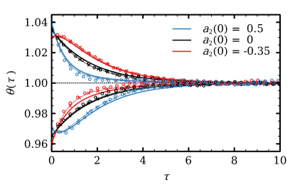
Figure 1: Evolution of the scaled temperature $\theta$ towards the steady state showing a clear Mpemba-like effect in a cooling process (top curves, with initial states $(\theta(0),a_{2}(0),a_{3}(0))=(1.04,0.5,-0.071)$, $(1.035,0,0)$ and $(1.03,-0.35,-0.375)$) and an inverse Mpemba-like effect in a heating process (bottom curves, with initial states $(\theta(0),a_{2}(0),a_{3}(0))=(0.97,0.5,-0.071)$, $(0.965,0,0)$ and $(0.96,-0.35,-0.375)$). Solid lines represent the exact solution, open circles correspond to MD, and dotted lines with crosses refer to DSMC simulations.

As we can see, our results exhibit an excellent agreement between the three independent methods, clearly displaying the ME in both the cooling and heating processes (the latter referred to as inverse ME). In effect, curve crossings between transients are clearly observed, in this case at very early times (before $\tau\sim 1$, i.e., before all particles have statistically had the chance to collide once after initialization).

For the cooling variant ($T(0)^{\mathrm{further}}>T(0)^{\mathrm{closer}}>T^{\mathrm{st}}$), we have represented the triplets $(1.04,0.5,-0.071)$, $(1.035,0,0)$ and $(1.03,-0.35,-0.375)$, whereas for the heating protocol ($T^{\mathrm{st}}>T(0)^{\mathrm{closer}}>T(0)^{\mathrm{further}}$) we have used the triplets $(0.96,0.5,-0.071)$, $(0.965,0,0)$ and $(0.97,-0.35,-0.375)$. Notice that the relaxation curve of the initial state whose temperature is furthest from the stationary value also crosses the one having intermediate Maxwellian initial state. This is an interesting result that indicates that the initial conditions further away from the steady state can also produce an ME relative to an initial state that resembles a microscopic equilibrium state.

We analyze now to what extent the ME is observable in a granular gas of viscoelastic particles. For this, we determine, from integration of equations (8)-(10), the ratio $\Delta\theta(0)/\Delta a_{2}(0)$, where $\Delta\theta(0)\equiv(T_{A}(0)-T_{B}(0))/T^{\mathrm{st}}$ and $\Delta a_{2}(0)\equiv a_{2A}(0)-a_{2B}(0)$ as a function of the dissipative coefficient $\gamma_{\nu}$. Results are displayed in Figure 2, where we can see there is a wide region of the parameter space in which the ME is present. Much like in the case of a gas of hard spheres, the Mpemba region grows as inelasticity increases ($\gamma_{\nu}=0$ is the perfectly elastic collision limit, and inelasticity grows as $\gamma_{\nu}$) but here, distinctively, the width of the Mpemba region for higher inelasticities soon reaches an asymptotic value and thus increasing inelasticity stops yielding wider Mpemba regions. Moreover, the ME is in general smaller for viscoelastic particles ($\Delta\theta(0)/\Delta a_{2}(0)<0.02$, even for higher inelasticities) which is less than $25\%$ the size of the ME that has been detected at high inelasticities in granular gases of hard spheresLasanta et al. (2017).

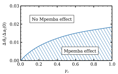
Figure 2: Theoretical phase diagram in the plane $\Delta\theta(0)/\Delta a_{2}(0)$ vs $\gamma_{\nu}$. The regions of the plane inside which there appears or does not appear the ME are separated by a curve, showing that there is a maximum of the parameter for which the ME can be observed.

IV Kovacs effect in a granular gas of viscoelastic particles

As we already know, the behavior of the KE is, in general, rather more complex in granular fluids than that of the original KE in a polymer layer Kovacs (1963); Kovacs et al. (1979). For instance, granular fluids display an upwards hump, analogously to the behavior encountered in the original work by Kovacs (and thus called henceforth normal hump); but also an anomalous hump downwards was found, this consisting in further cooling after the bath temperature is fixed during a cooling transient in systems with high inelasticities Prados and Trizac (2014); Trizac and Prados (2014). Furthermore, multiple –alternatively upwards and downwards– humps have been detected in granular fluids where particles have rotational degrees of freedom as well Lasanta et al. (2019). But, again, the question remains if the KE is really present in granular fluid experiments and, as we said, a first theoretical approach is to model grain collisions more realistically, via the viscoelastic model in this case.

(a)

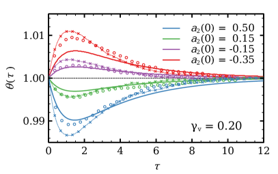
(b)

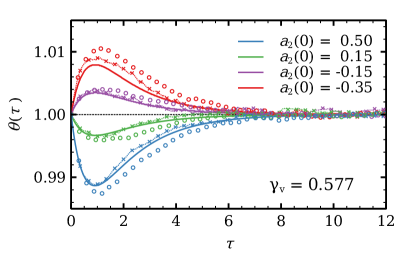
Figure 3: Theoretical (lines), MD simulation (open circles) and DSMC (dotted lines with crosses) results, showing the KE for (a) $\gamma_{\nu}=0.2$ and (b) $\gamma_{\nu}=0.577$.

Thus, in order to detect the KE in granular fluids with the (more realistic) viscoelastic model, we subject the system to a stochastic thermostat of intensity $\xi_{0}^{2}$, which is set so that $T(0)=T^{\mathrm{st}}(\xi_{0}^{2})$. In addition, the initial values of the cumulants, $a_{2}(0)$ and $a_{3}(0)$, are set to values very different from their steady state values (similarly to the ME case), so that the initial distribution function is far from its stationary form. Therefore, once the system is left to evolve, it will undergo a transient with the necessary time for the cumulants to approach their steady state values (which are known a priori since they only depend on the dissipation coefficient Dubey et al. (2013)).

But, since the system is already initially at its steady state temperature, any eventual departure during the transient of the granular temperature at later times should correspond to a Kovacs-like effect. This is potentially possible due to the strong coupling of the time evolution of the cumulants $a_{2}$ and $a_{3}$ and $T$ (see Equations (8)-(10)). And, as we will show, we have certainly observed the KE for wide ranges of the parameter space for viscoelastic particles.

(a)

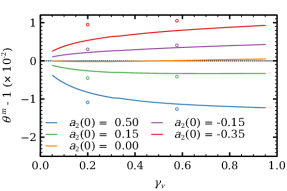
(b)

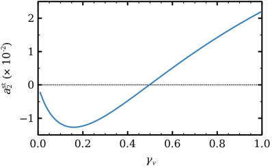
Figure 4: (a) Size of the theoretical (lines) and MD simulation (open circles) hump in the granular temperature evolution as a function of $\gamma_{\nu}$ for different values of $a_{2}(0)$ and $a_{3}(0)$ (as reported in Table 1). The sign of the kurtosis difference $a_{2}(0)-a_{2}^{\mathrm{st}}$ determines whether the evolution curves exhibit an upwards ($a_{2}(0)<a_{2}^{\mathrm{st}}$) or downwards ($a_{2}(0)>a_{2}^{\mathrm{st}}$) hump. (b) The theoretical stationary kurtosis $a_{2}^{\mathrm{st}}$ is a non-constant function of the inelasticity parameter $\gamma_{\nu}$.

Table 1: Initial values of the cumulants $a_{2}$ and $a_{3}$ used in Figure 3. The stationary values of the cumulants are $a_{2}^{\mathrm{st}}=-0.012312$ and $a_{3}^{\mathrm{st}}=-0.003249$ for $\gamma_{\nu}=0.2$ and $a_{2}^{\mathrm{st}}=0.003957$ and $a_{3}^{\mathrm{st}}=-0.002768$ for $\gamma_{\nu}=0.577$.

$a_{2}(0)$	0.5	0.15	$-0.15$	$-0.35$
$a_{3}(0)$	$-0.07143$	0.05357	$-0.11786$	$-0.375$

We illustrate this in Figure 3, in panel (a) for low inelasticity ($\gamma_{\nu}=0.2$) and in (b) for a more inelastic gas ($\gamma_{\nu}=0.577$); the different values of $a_{2}(0)$ and $a_{3}(0)$ used in these curves are summarized in Table 1. For the two values of $\gamma_{\nu}$ used here, strong and remarkably similar KEs are observed, as Figure 3 shows. Note that the hump sign for the curves present matches that of the difference $a_{2}^{\mathrm{st}}-a_{2}(0)$; i.e., the hump is downwards for $a_{2}^{\mathrm{st}}-a_{2}(0)<0$ and upwards for $a_{2}^{\mathrm{st}}-a_{2}(0)>0$. This behavior is identical in both dissipative coefficient values analyzed here ($\gamma=0.577$, which has high dissipation and $\gamma_{v}=0.2$, with small dissipation). Therefore, it does not appear to be essentially determined by inelasticity. This is much in contrast with the behavior for hard spheres, where a clear hump sign transition for the coefficient of restitution critical value $\alpha_{c}=1/\sqrt{2}\sim 0.7$ was reported in the bibliography Prados and Trizac (2014). It is also interesting to notice that, in general, there is a good agreement between theory and simulation, so it is guaranteed that the result observed here is not an artifact of the approximations used in the theoretical approach.

In order to further clarify this behavior, we analyze in Figure 4(a) the evolution of the signed hump size (here represented as $\theta^{m}-1$ where $\theta^{m}\equiv T^{m}/T^{\mathrm{st}}$ and $T^{m}$ is the maximum/minimum value achieved by the granular temperature during the transient), for different initial values of the cumulants $a_{2}(0),a_{3}(0)$, vs. the dissipative coefficient (as summarized in Table 1). Results show that the hump sign does not depend essentially on dissipation upon collision. Notice that each curve remains with the same hump sign whether dissipation is high or low. This corroborates that the behavior of this memory effect for viscoelastic particles and, thus, very possibly in experiments, is essentially different from that in the less realistic hard sphere collisional model.

However, a subtle sign transition for the $a_{2}(0)=0$ curve can be observed at $\gamma_{\nu}\sim 0.45$ (orange line in Figure 4(a)). We plot in Figure 4(b), the difference $a_{2}^{\mathrm{st}}-a_{2}(0)$ for the case $a_{2}(0)=0$ (i.e., $a_{2}^{\mathrm{st}}-a_{2}(0)=a_{2}^{\mathrm{st}}$). We note that, in effect, $a_{2}^{\mathrm{st}}$ changes sign at $\gamma_{\nu}\sim 0.45$. Moreover, Figure 4(b) shows that the sign of this difference matches the hump sign for all $\gamma_{\nu}$, by comparison with the corresponding curve in Figure 4(a), and therefore, that the hump sign is determined by the difference $a_{2}^{\mathrm{st}}-a_{2}(0)$. But, even more interestingly, we observe that curve $a_{2}(0)$ displays a Kovacs sign transition that is the opposite to the one reported for hard spheres; i.e., in a granular gas of viscoelastic particles the Kovacs hump is in the quasi-elastic collision limit.

Since, due to the scale in Figure 4 this detail is hard to grasp, we plot in Figure 5 the hump size for varying $a_{2}(0)$ and several dissipative coefficient ($\gamma_{\nu}$) values. The large panel helps to visualize that, regarding the hump sign, the initial value of $a_{2}(0)$ is indeed by far the most determining factor. Remarkably, it helps to figure also that it is not the only factor, since the hump changes sign at slightly different values of $a_{2}(0)$ for different values of the dissipative coefficients (see inset). This feature is also exclusive of our system and does not appear in granular gases of hard spheres, for which the transition is fixed at coefficient of restitution $\alpha_{c}=1/\sqrt{2}$ for all thermal protocols; i.e., all initial state cases (see Figure 9 in Trizac and Prados (2014), for instance). Figure 5 inset helps to visualize also that the hump sign, for $a_{2}(0)\sim 0$, changes from negative for quasi-elastic collisions (smaller $\gamma_{\nu}$ values) to positive sign for highly inelastic collisions (larger $\gamma_{\nu}$ values). This is evident since, at $a_{2}(0)=0$, the curves for more elastic collisions ($\gamma_{\nu}=0.1;\gamma_{\nu}=0.2$) have a negative hump whereas the curves for more inelastic gases ($\gamma_{\nu}=0.8;\gamma_{\nu}=0.9$) have a positive hump.

Moreover, this is a striking result since it implies that the most dissipative granular gases of viscoelastic particles, and not the quasi-elastic ones, display a thermal memory more similar to that of equilibrium systems.

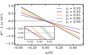
Figure 5: The signed hump size ($\theta^{m}-1$) vs. $a_{2}(0)$ for different dissipative coefficient values ($\gamma_{\nu}$ in this case).

V Discussion

We have analysed the presence of two memory effects in a system of identical viscoelastic spherical grains, where the coefficient of restitution depends on the relative velocities of pairs of colliding particles Dubey et al. (2013). We subject the granular gas to thermal protocols by means of a homogeneous stochastic force or thermostat. We have observed that, under appropriate conditions, the temperature relaxation curves may display a rich phenomenology of memory effects; i.e., both the ME and the KE are observed in granular gases of viscoelastic particles, like in their analogs with simpler, less realistic collisional models.

Nevertheless, we have reported profound differences in the behavior of both memory effects with respect to inelastic hard spheres. Namely, the ME is significantly smaller for viscoelastic particles, and the increase of the effect for more inelastic particles is much more limited.

It is interesting to note that the KE behavior that we observed is qualitatively different from the one reported for granular gases of smooth hard particles, as described in the previous section. Much like in the case of a granular gas of hard particles, we observe here downwards and upwards KEs, but the hump sign is mainly –but not uniquely– controlled here by the initial values of the cumulants, whereas for smooth hard particles the sign transition is driven by inelasticity Prados and Trizac (2014). Moreover, the hump sign is always positive for more inelastic collisions for all initial values of the cumulants, except in the region $a_{2}(0)\sim 0$. Indeed, a hump sign transition with respect to the dissipative coefficient has been detected for $a_{2}(0)\sim 0$, from positive hump –for more inelastic particles– to negative hump –for more elastic particles–. Strikingly as well, the critical value of the dissipative coefficient for hump sign transition slightly varies for different initial conditions, contrary to the case of hard particles, where the transition has been reported to occur at the fixed value of coefficient of restitution $\alpha_{c}=1/\sqrt{2}$ for all initial conditions.

VI Conclusion

We have shown that the ME and/or KE appear when a system is relaxing towards a stationary state and the initial values of the cumulants are far from their steady state values. We also demostrate numerically that this is due to the existing coupling between cumulants and temperature, which induces its direction. Furthermore, both memory effects arising from a coupling of the granular temperature with $a_{2}$ and $a_{3}$ represents a step towards a unifying description of memory effects in the context of granular dynamics and opens new avenues for the study of more sophisticated systems like the ones composed by anisotropic particles Gómez-Solano, Blokhuis, and Bechinger (2016); Mallory, Valeriani, and Cacciuto (2018); Lasanta, Torrente, and López de Haro (2019).

In summary, thermal memory effects are intrinsically present in a granular gas whose particle collisions are described with the more realistic viscoelastic model, but with important differences with respect to simpler collisional models. In fact, this is another proof that the ME is not a theoretical artifact depending on a particular model. Therefore, and since these memory effects are ubiquitous in granular fluid theoretical studies, we suggest they should be detectable in laboratory experiments but also with important differences with results reported in previous theoretical developments.

The present work is thus a step towards a more realistic description of memory effects in granular dynamics, to be compared with the experimental behavior in a future work, in the same train of thought that both effects have been found in single particle experiments. Insight into thermal relaxation will improve the understanding of the granular dynamics, whose transport properties are known to be highly dependent on temperature. Since grains are a component present in a variety of industrial processes Goldhirsch (2003); Brilliantov and Pöschel (2004), applied research is expected to benefit from these results as well.

Data Availability Statement

The data that support the findings of this study are available from the corresponding author upon reasonable request.

*

Appendix A Numerical methods

As explained in the body of the text, we have carried out our study by using three complementary techniques: numerical solution (by means of the MATLAB package) of the time differential equation system of the first three moments of the distribution function, accounting for the required approximations, molecular dynamics (MD) simulations Pöschel and Schwager (2005), and numerical solution of the kinetic equation obtained through the Direct Simulation Monte Carlo method (DSMC) Bird (2004).

Solutions to equations (8)-(10) were numerically approximated using a forward Euler method with a time step $\Delta\tau=0.001$. The method’s expected first order of convergence was numerically verified as follows: let $u$ denote the solution to one of the differential equations, and let $u_{h}$ be the numerical approximation to $u$ using time steps of length $h$. As the actual solution is not known beforehand, for any length $h$ we shall store the approximated values at times $\tau=n\Delta\tau$, for $n=0,1,2,\ldots$, into a vector $v_{h}$. That is, $v_{h}^{n}\approx u(n\Delta\tau)$. If the method has an order of convergence $p$, then $\max_{n}|u(n\Delta\tau)-v_{h}^{n}|\leq Ch^{p}$, for some constant $C>0$. Since $u$ is not available, the order can be estimated by means of successive refinements of the time step length:

$$\frac{\|v_{\Delta\tau}-v_{\Delta\tau/2}\|_{\infty}}{\|v_{\Delta\tau/2}-v_{\Delta\tau/4}\|_{\infty}}=2^{p}+O(\Delta\tau),$$ (A.14)

where $\|v\|_{\infty}=\max_{n}|v^{n}|$. Using this, the order of convergence $p\approx 1$ has been consistently recovered for all the experiments described heretofore. Moreover, a time step $\Delta\tau\leq 0.01$ was sufficient in all cases. Hence $\Delta\tau=0.001$ lies well within the stability region of the method.

MD computer simulation is a powerful tool that allows knowing the spatial coordinates of every constituent particle in the molecular gas at all times, an option that, though time-consuming, is barely accessible through experiments. It numerically solves Newton’s equations of motion for all particles by accounting for forces and torques acting on them and by incorporating realistic values for the parameters describing the material properties.

In (event-driven) MD simulations, collisions are binary and of infinitesimal duration, and the dynamics is regulated by a sequence of discrete events. The system particles follow known ballistic trajectories during the time intervals between collisions, allowing the computation of particle positions on the next collision in a single step. The MD algorithm can be summarized as:

1. Initialization of positions and velocities for all $N$ particles at time $t=0$.

2. Determination of the time $t_{next}$ at which the next collision occurs and the particles $i$ and $j$ involved in such a collision.

3. Update of positions of all particles at time $t_{next}$.

4. Update of velocities of the two colliding particles, according to the system collision rule, in our case given by:

   $$v_{i}^{\prime}=v_{i}-\dfrac{1+\epsilon}{2}\left(v_{ij}\cdot e_{ij}\right)e_{ij},$$ (A.15)

   $$v_{j}^{\prime}=v_{j}-\dfrac{1+\epsilon}{2}\left(v_{ij}\cdot e_{ij}\right)e_{ij}.$$ (A.16)

   Here, the not-primed and primed $v_{k}$s refer to pre- and post-collisional velocities, respectively, $\epsilon$ is the restitution coefficient given in equation (2), $v_{ij}=v_{i}-v_{j}$ is the relative velocity and $e_{ij}$ is a unit vector pointing from the center of mass of particle $j$ to that of particle $i$ at the instant of the collision.

Steps (ii)–(iv) are repeated until a steady state, which is defined by a target temperature provided by a thermostat, is reached.

In our experiments, the MD data sets have been obtained out of simulation runs for systems with dimensionless number density $n\sigma^{3}=0.01$, with $n$ the number of particles per volume unit, which are composed of particles of mass and diameter equal to 1. We have considered periodic boundary conditions to mimic an infinitely extended system. In the ME study, we have used a coefficient of restitution with dissipative coefficient $\gamma_{\nu}=0.577$ and an appropriate gamma density function for the initial velocity distribution Hogg and Craig (1978) to recreate the selected values of $a_{2}$. Hence, the values of $a_{3}$ are the ones associated to such a distribution. For ME simulations, we have averaged over $10^{3}$ trajectories. On the other hand, more computational trajectories are needed to evince the more subtle KE for some of the values of $\gamma_{\nu}$, thus we have averaged over $10^{4}$ trajectories for each of the reported dissipative coefficient values, $\gamma_{\nu}=0.20$ and $0.577$.

As a brief description of the DSMC method, one must remember that the dynamics of the system is determined by the Boltzmann equation:

$$\left[\partial_{t}+(v\cdot\gradient)\right]f+\frac{1}{m}\frac{\partial}{\partial v}\cdot(Ff)=J[f,f].$$ (A.17)

To solve this equation, rather than exactly calculating the outcome of every impact, the Monte Carlo approach generates collisions stochastically. These are not necessarily real collisions but outcome makes the system behaviour be correct around mean free path length scales Alexander and Garcia (1997).

The standard algorithm (using Bird’s no-time-counter, NTC, scheme Bird (1994)) consists of the following steps:

1. Initialization: As with MD, $N$ particles are randomly created and distributed (with positions $r_{i}$) among the simulation volume. One key difference though is that there is no need to care for overlapping particles since the computed collisions will not be physically exact. A large number of particles can be simulated in DSMC, typically from $10^{4}$ to $10^{8}$. However, if the number of grains is fewer than about $20$ per cubic mean free path the results may not be accurate ($\lambda=(\sqrt{2}\pi\sigma^{2}n)^{-1}$ in a dilute gas). Besides positions, each particle is given an initial velocity $v_{i}$, usually extracted from a Maxwellian distribution function.

2. Collision: A random number of particles are selected for colliding; this selection method is derived from kinetic theory. For inhomogeneus systems, particles very distant from each other should not interact, so the simulation box should be divided into cells and collisions are evaluated only among particles of the same sub-cell (this is not our case, there are no long-range gradients in our system that require grid sub-division). This set of random representative collisions is processed at each time step $\Delta t$ (which is set at a value much smaller than the mean free time); only the magnitude of the relative velocity between particles is used to evaluate the probability of a collision, regardless of their positions. Therefore, the probability of a collision between a pair of particles is:

   $$P_{col}(i,j)=\frac{\absolutevalue{v_{ij}}}{\sum_{m=1}^{N_{c}}\sum_{n=1}^{m-1}\absolutevalue{v_{mn}}},$$ (A.18)

   where $N_{c}$ is the number of particles in that sub-cell.

   Since using previous equation is very inneficient due to the iteration over every particle in the denominator, another method is used for selecting which collisions to evaluate.

   First, a random uniform value $r\in(0,1)$ is generated, then an aleatory pair of particles $i,j$ is selected. That pair is considered to undergo a collision if the following condition is met:

   $$\frac{\absolutevalue{v_{ij}}}{v_{\mathrm{r,max}}}>r,$$ (A.19)

   where $v_{\mathrm{r,max}}$ is the maximum relative speed in the cell. If the pair $i,j$ is accepted, post-collisional velocities are computed for that pair. Finally, this algorithm is repeated until a certain number $M_{col}$ of collisions has been accepted and processed. The value of $M_{col}$ is costly to calculate, thus, the algorithm should be repeated a number of times given by $M_{cand}$, for a hard-sphere model:

   $$M_{cand}=\frac{N_{c}^{2}\pi\sigma^{2}v_{\mathrm{r,max}}\Delta t}{2V_{c}},$$ (A.20)

   where $V_{c}$ is the volume of the cell. Special attention must be paid to the estimation of $v_{\mathrm{r,max}}$, which is very computationally expensive, so usually $v_{\mathrm{r,max}}$ is indirectly overestimated by multiplying $\langle v\rangle$ by a certain factor.

These steps are repeated until the system reaches a steady state; to achieve this, a thermostat has been implemented following the methods described in Montanero and Santos (2000b). Finally, the viscoelastic behaviour of our particles has been encoded in the operator $J[f,f]$ which defines the outcome of collisions. In this paper, for DSMC simulations we have used 100 statistically independent replicas with $N=2\times 10^{5}$ particles each, a number which has proven to yield small errors in other works Maltsev (2011).

References

- Mpemba and Osborne (1969) E. B. Mpemba and D. G. Osborne, “Cool?” Phys. Educ. 4, 172–175 (1969).
- Kovacs et al. (1979) A. J. Kovacs, J. J. Aklonis, J. M. Hutchinson, and A. R. Ramos, “Isobaric volume and enthalpy recovery of glasses. ii. a transparent multiparameter theory,” J. Polym. Sci. B 17, 1097–1162 (1979).
- Vega Reyes and Lasanta (2019) F. Vega Reyes and A. Lasanta, “Time evolution of the microscopic state of an athermal fluid,” in AIP Conference Proceeding, 31st International Symposium on Rarefied Gas Dynamics, Vol. 2132, 080004 (2019) https://doi.org/10.1063/1.5119585 .
- Keim et al. (2019) N. C. Keim, J. D. Paulsen, Z. Zeravcic, S. Sastry, and S. R. Nagel, “Memory formation in matter,” Rev. Mod. Phys. 91, 035002 (2019).
- Lasanta et al. (2017) A. Lasanta, F. Vega Reyes, A. Prados, and A. Santos, “When the hotter cools more quickly: Mpemba effect in granular fluids,” Phys. Rev. Lett. 119, 148001 (2017).
- Lasanta et al. (2019) A. Lasanta, F. Vega Reyes, A. Prados, and A. Santos, “On the emergence of large and complex memory effects in nonequilibrium fluids,” New J. Phys. 21, 033042 (2019).
- Goldhirsch (2003) I. Goldhirsch, “Rapid granular flows,” Annu. Rev. Fluid Mech. 35, 267–293 (2003).
- Burridge and Hallstadius (2020) H. C. Burridge and O. Hallstadius, “Observing the Mpemba effect with minimal bias and the value of the Mpemba effect to scientific outreach and engagement,” Proc. R. Soc. A 476, 20190829 (2020).
- Lu and Raz (2017) Z. Lu and O. Raz, “Nonequilibrium thermodynamics of the Markovian Mpemba effect and its inverse,” Proc. Natl. Acad. Sci. U. S. A. 114, 5083–5088 (2017).
- Greaney et al. (2011) P. A. Greaney, G. Lani, G. Cicero, and J. C. Grossman, “Mpemba-like behavior in carbon nanotube resonators,” Metall. Mater. Trans. A 42, 3907–3912 (2011).
- Ahn et al. (2016) Y. H. Ahn, H. Kang, D. Y. Koh, and H. Lee, “Experimental verifications of Mpemba-like behaviors of clathrate hydrates,” Korean J. Chem. Eng. 33, 1903–1907 (2016).
- Yang and Hou (2020) Z.-Y. Yang and J.-X. Hou, “Non-Markovian Mpemba effect in mean-field systems,” Phys. Rev. E 101, 052106 (2020).
- Biswas et al. (2020) A. Biswas, V. V. Prasad, O. Raz, and R. Rajesh, “Mpemba effect in driven granular Maxwell gas,” Phys. Rev. E 102, 012906 (2020).
- Gómez González, Khalil, and Garzó (2020) R. Gómez González, N. Khalil, and V. Garzó, “Mpemba-like effect in driven binary mixtures,” arXiv:2010.14215v2 (2020).
- Santos and Prados (2020) A. Santos and A. Prados, “Mpemba effect in molecular gases under nonlinear drag,” Phys. Fluids 32, 072010 (2020).
- Takada, Hayakawa, and Santos (2021) S. Takada, H. Hayakawa, and A. Santos, “Mpemba effect in intertial suspensions,” Phys. Rev. E 103, 032901 (2021).
- Klich et al. (2019) I. Klich, O. Raz, O. Hirschberg, and M. Vucelja, “Mpemba index and anomalous relaxation,” Phys. Rev. X 9, 021060 (2019).
- Gal and Raz (2020) A. Gal and O. Raz, “Precooling strategy allows exponentially faster heating,” Phys. Rev. Lett. 124, 060602 (2020).
- Nava and Fabrizio (2019) A. Nava and M. Fabrizio, “Lindblad dissipative dynamics in the presence of phase coexistence,” Phys. Rev. B 100, 125102 (2019).
- Baity-Jesi et al. (2019) M. Baity-Jesi, E. Calore, A. Cruz, L. A. Fernandez, J. M. Gil-Narvión, A. Gordillo-Guerrero, D. Iñiguez, A. Lasanta, A. Maiorano, E. Marinari, V. Martin-Mayor, J. Moreno-Gordo, A. M. Sudupe, D. Navarro, G. Parisi, S. Perez-Gaviro, F. Ricci-Tersenghi, J. J. Ruiz-Lorenzo, S. F. Schifano, B. Seoane, A. Tarancón, R. Tripiccione, D. Yllanes, and et al., “The Mpemba effect in spin glasses is a persistent memory effect,” Proc. Natl. Acad. Sci. U. S. A. 116, 15350–15355 (2019).
- Gijón, Lasanta, and Hernández (2019) A. Gijón, A. Lasanta, and E. R. Hernández, “Paths towards equilibrium in molecular systems: the case of water,” Phys. Rev. E. 100, 032103 (2019).
- Kumar and Bechhoefer (2020) A. Kumar and J. Bechhoefer, “Exponentially faster cooling in a colloidal system,” Nature 584, 64 (2020).
- Kumar, Chetrite, and Bechhoefer (2021) A. Kumar, R. Chetrite, and J. Bechhoefer, “Anomalous heating in a colloidal system,” arXiv:2104.12899 (2021).
- Carollo, Lasanta, and Lesanovsky (2021) F. Carollo, A. Lasanta, and I. Lesanovsky, “Exponentially accelerated approach to stationarity in markovian open quantum systems through the mpemba effect,” arXiv:2103.05020 (2021).
- Gómez González and Garzó (2020) R. Gómez González and V. Garzó, “Anomalous Mpemba effect in binary molecular suspensions,” arXiv:2011.13237 (2020).
- Lapolla and Godec (2020) A. Lapolla and A. c. v. Godec, “Faster uphill relaxation in thermodynamically equidistant temperature quenches,” Phys. Rev. Lett. 125, 110602 (2020).
- Van Vu and Hasewaga (2021) T. Van Vu and Y. Hasewaga, “Toward conjecture: Warming is faster than cooling,” arXiv:2102.07429 (2021).
- Manikandan (2021) S. K. Manikandan, “Faster uphill relaxation of a two-level quantum system,” arXiv:2102.06161 (2021).
- Maynar, García de Soria, and Brey (2019) P. Maynar, M. I. García de Soria, and J. J. Brey, “Homogeneous dynamics in a vibrated granular monolayer,” J. Stat. Mech.: Theory Exp. 2019, 093205 (2019).
- Torrente et al. (2019) A. Torrente, M. A. López-Castaño, A. Lasanta, F. Vega Reyes, A. Prados, and A. Santos, “Large Mpemba-like effect in a gas of inelastic rough hard spheres,” Phys. Rev. E 99, 060901(R) (2019).
- Walton (1992) O. R. Walton, “Particulate two-phase flow,” (Butterworth-Heinemann, Boston, 1992) Chap. Numerical simulation of inelastic, frictional particle-particle interactions, pp. 884–911.
- Foerster et al. (1994) S. F. Foerster, M. Y. Louge, H. Chang, and K. Allis, “Measurements of the collision properties of small spheres,” Phys. Fluids. 6, 1108–1115 (1994).
- Grasselli, Bossis, and Morini (2015) Y. Grasselli, G. Bossis, and R. Morini, “Translational and rotational temperatures of a 2D vibrated granular gas in microgravity,” Eur. Phys. J. E. Soft Matter 38, 93 (2015).
- Maw, Barber, and Fawcett (1981) N. Maw, J. R. Barber, and J. N. Fawcett, “The role of elastic tangential compliant in oblique impact,” ASME J. Lub. Technol. 103, 74–80 (1981).
- Gugan (2000) D. Gugan, “Inelastic collision and the hertz theory of impact,” Am. J. Phys. 68, 920 (2000).
- Louge (2009) M. Louge, “Research on the impact of small spheres at cornell university,” http://grainflowresearch.mae.cornell.edu/impact/impact.html (1994–2009).
- Brilliantov et al. (1996) N. V. Brilliantov, F. Spahn, J. M. Hertzsch, and T. Pöschel, “Model for collisions in granular gases,” Phys. Rev. E 53, 5382–5392 (1996).
- Brilliantov and Pöschel (2004) N. Brilliantov and T. Pöschel, Kinetic Theory of Granular Gases (Oxford University Press, 2004).
- Kovacs (1963) A. J. Kovacs, “Transition vitreuse dans les polymères amorphes. étude phénoménologique,” Fortschr. Hochpolymer–Forsch. 3, 394–507 (1963).
- Mossa and Sciortino (2004) S. Mossa and F. Sciortino, “Crossover (or kovacs) effect in an aging molecular liquid,” Phys. Rev. Lett. 92, 045504 (2004).
- Aquino, Leuzzi, and Nieuwenhuizen (2006) G. Aquino, L. Leuzzi, and T. M. Nieuwenhuizen, “Kovacs effec in a model for a fragile glass,” Phys. Rev. B 73, 094205 (2006).
- Banik and McKenna (2018) S. Banik and G. B. McKenna, “Isochoric structural recovery in molecular glasses and its analog in colloidal glasses,” Phys. Rev. E 97, 062601 (2018).
- Song et al. (2020) L. Song, W. Xu, J. Huo, F. Li, L.-M. Wang, M. D. Ediger, and J.-Q. Wang, “Activation entropy as a key factor controlling the memory effect in glasses,” Phys. Rev. Lett. 125, 135501 (2020).
- Kürsten, Sushkov, and Ihle (2017) R. Kürsten, V. Sushkov, and T. Ihle, “Giant kovacs-like memory effect for active particles,” Phys. Rev. Lett. 119, 188001 (2017).
- Militaru et al. (2021) A. Militaru, A. Lasanta, M. Frimmer, L. L. Bonilla, L. Novotny, and R. A. Rica, “Kovacs memory effect with an optically levitated nanoparticle,” arXiv:2103.14412 (2021).
- Plata and Prados (2017) C. Plata and A. Prados, “Kovacs-like memory effect in athermal systems: linear response analysis,” Entropy 19, 539 (2017).
- Prados and Trizac (2014) A. Prados and E. Trizac, “Kovacs-like memory effect in driven granular gases,” Phys. Rev. Lett. 112, 198001 (2014).
- Trizac and Prados (2014) E. Trizac and A. Prados, “Memory effect in uniformly heated granular gases,” Phys. Rev. E. 90, 012204 (2014).
- Brey et al. (2014) J. J. Brey, M. I. García de Soria, P. Maynar, and V. Buzón, “Memory effects in the relaxation of a confined granular gas,” Phys. Rev. E 90, 032207 (2014).
- Sánchez-Rey and Prados (2020) B. Sánchez-Rey and A. Prados, “Linear response in the uniformly heated granular gas,” arXiv:2010.10196 (2020).
- Dubey et al. (2013) A. K. Dubey, A. Bodrova, S. Puri, and N. Brilliantov, “Velocity distribution function and effective restitution coefficient for a granular gas of viscoelastic particles,” Phys. Rev. E 87, 062202 (2013).
- Montanero and Santos (2000a) J. M. Montanero and A. Santos, “Computer simulation of uniformly heated granular fluids,” Granular Matt. 2, 53–64 (2000a).
- Sonine (1880) N. Sonine, “Recherches sur les fonctions cylindriques et le développement des fonctions continues en série,” Math Ann. 16, 1 (1880).
- van Noije and Ernst (1998) T. P. C. van Noije and M. H. Ernst, “Velocity distributions in homogeneous granular fluids: the free and the heated case,” Granul. Matter 1, 57–64 (1998).
- Chamorro, Vega Reyes, and Garzó (2013) M. G. Chamorro, F. Vega Reyes, and V. Garzó, “Homogeneous steady states in a granular fluid driven by a stochastic bath with friction,” J. Stat. Mech.: Theory and Experiment 2013, P07013 (2013).
- Vega Reyes, Santos, and Kremer (2014) F. Vega Reyes, A. Santos, and G. M. Kremer, “Role of roughness on the hydrodynamic homogeneous base state of inelastic spheres,” Phys. Rev. E 89, 020202(R) (2014).
- Pashine et al. (2020) N. Pashine, D. Hexner, A. J. Liu, and S. R. Nagel, “Directed aging, memory, and nature’s greed,” Science Adv. 5, eaax4215 (2020).
- Schindler and Rohwer (2020) T. Schindler and C. M. Rohwer, “Ballistic propagation of density correlations and excess wall forces in quenched granular media,” Phys. Rev. E 102, 052901 (2020).
- Bird (2004) G. I. Bird, Molecular Gas Dynamics and the Direct Simulation of Gas Flows (Clarendon, Oxford, 2004).
- (60) We use for this the Intel MKL performance libraries.
- (61) Notice that, contrary to the case of inelastic smooth hard particles [ref. 31] the cumulant for viscoelastic particles is in general not negligible in comparison with [ref. 17] and for this reason we consider both cumulants in the relaxation process.
- Gómez-Solano, Blokhuis, and Bechinger (2016) J. R. Gómez-Solano, A. Blokhuis, and C. Bechinger, “Dynamics of self-propelled janus particles in viscoelastic fluids,” Phys. Rev. Lett. 116, 138301 (2016).
- Mallory, Valeriani, and Cacciuto (2018) S. A. Mallory, C. Valeriani, and A. Cacciuto, “An active approach to colloidal self-assembly,” Ann. Rev. Phys. Chem. 69, 59–79 (2018).
- Lasanta, Torrente, and López de Haro (2019) A. Lasanta, A. Torrente, and M. López de Haro, “Induced correlations and rupture of molecular chaos by anisotropic dissipative janus hard disks,” Phys. Rev. E 100, 052128 (2019).
- Pöschel and Schwager (2005) T. Pöschel and T. Schwager, Computational Granular Dynamics (Springer-Verlag Berlin Heidelberg, 2005).
- Hogg and Craig (1978) R. V. Hogg and A. T. Craig, Introduction to mathematical statistics (Macmillan Publishing, New York, 1978) pp. 103–108.
- Alexander and Garcia (1997) F. J. Alexander and A. L. Garcia, “The Direct Simulation Monte Carlo Method,” Comp. in Phys. 11, 588 (1997).
- Bird (1994) G. A. Bird, “Molecular Gas Dynamics and the Direct Simulation of Gas Flows,” (1994).
- Montanero and Santos (2000b) J. M. Montanero and A. Santos, “Computer simulation of uniformly heated granular fluids,” Gran. Matt. 2, 53–64 (2000b).
- Maltsev (2011) R. V. Maltsev, “On the selection of the number of model particles in DSMC computations,” AIP Conference Proceedings 1333, 289–294 (2011).