Unsighted deconvolution ghost imaging

Abstract

Ghost imaging (GI) is an unconventional imaging method that retrieves the image of an object by correlating a series of known illumination patterns with the total reflected (or transmitted) intensity. We here demonstrate a scheme which can remove the basic requirement of knowing the incident patterns on the object, enabling GI to non-invasively image objects through turbid media. As an experimental proof, we project a set of patterns towards an object hidden inside turbid media that scramble the illumination, making the patterns falling on the object completely unknown. We theoretically prove that the spatial frequency of the object is preserved in the measurement of GI, even though the spatial information of both the object and the illumination is lost. The image is then reconstructed with phase retrieval algorithms.

I Introduction

Different than the conventional imaging methods that rely on the first-order interference (typically using lenses), Ghost imaging(GI) exploits the second-order correlation to reconstruct an imagePittman et al. (1995), bringing advantages such as better resistance to turbulenceYang et al. (2016), high detection sensitivityMorris et al. (2015); Zhao et al. (2019), lensless imaging capabilityScarcelli et al. (2006), and broad adaptability for different scenariosPeng et al. (2015); Liu and Zhang (2017); Aspden et al. (2015). Therefore, GI has drawn a lot of attention during the past two decades, invoking a lot potential applications in various fields ranging from optical imagingGong et al. (2016), X-ray imagingPelliccia et al. (2016); Yu et al. (2016); Zhang et al. (2018), to atomic sensingKhakimov et al. (2016); Baldwin et al. (2017).

A typical GI setup consists of a test and a reference arms. In the test arm, an object is illuminated by a temporally and spatially changing light field. The reflected or transmitted light from the object is collected by a bucket detector with no spatial-resolving capability. The reference arm is used to measure the variance of the light field on a conjugate plane of the object plane, i.e., the illumination patterns. The correlation between the patterns and the bucket signal results in the image of the object. Computational ghost imaging (CGI) is a setup that removes the reference arm. Instead, it pre-calculates or pre-determines the light patterns on the object plane. Since the bucket detector is simply used for collecting all the light from the object, the test arm is resistant to turbulence or strong light scattering. Most works focused on investigating GI with a turbid medium placed between an object and a bucket detectorTajahuerce et al. (2014); Yang et al. (2016); Bai et al. (2017); Ye et al. (2020). GI requires the light patterns illuminating the object be well determined. If the illumination patterns are disturbed by weak scattering, the reconstruction quality will be degradedBina et al. (2013); Li et al. (2020). If a strong-scattering medium placed between the source and the object totally scrambles the patterns, GI will fail to recover an imageGong and Han (2011); Yang et al. (2016). Although there was an approach that used ghost imaging configuration to image objects hidden behind turbid media, it exploited the non-Gaussion correlation which results in the resolution of the same order as the distance from the front surface of a turbid medium to the object (the width of the medium plus the distance between object to the medium)Paniagua-Diaz et al. (2019). If this distance is several centimeters, it could not resolve structures smaller than a centimeter, limiting its applications. This is different from a typical GI scheme which is based on Gaussian statistics and whose resolution depends on the grain size of the illuminating patterns on the objectCai and Zhu (2005); Fayard et al. (2015).

We here propose a new scheme that allows one to perform ghost imaging without knowing the illumination patterns on the object. The imaging resolution still obeys the same rule in GI: it is determined by the average grain size of the illumination patterns. Our method enables GI to non-invasively image an object completely hidden inside opaque media. In the following, We demonstrate a GI experiment with an opaque medium presented between the light source and an object. The image is deconvolved from the correlation between the preset patterns of the source and the bucket detections, after applying a phase retrieval algorithm. A theoretical proof is provided in the following section.

II Experiment

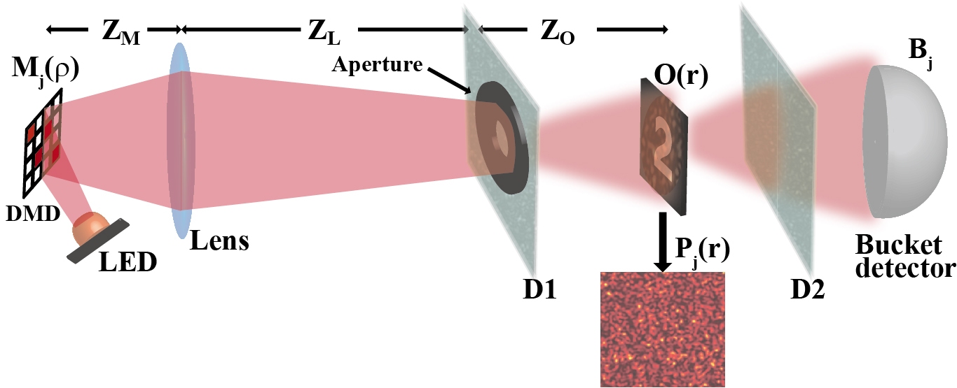
Figure 1: Schematic of ghost imaging for an object hidden between two opaque diffusers. A DMD (Digital Micromirror Device) displays a sequence of patterns $\{M_{j}({\boldsymbol{\rho}})\}$. A LED bulb and a lens are used to project the patterns towards an object hidden behind a diffuser (D1). D1 scatters the illuminating light and generates random speckles $\{P_{j}({\boldsymbol{r}})\}$ on object $O({\boldsymbol{r}})$. A small aperture with a diameter of $D\simeq 6\;mm$ is placed right in front of D1. A bucket detector measures the transmitted light from the object passing through another diffuser (D2), giving the bucket signals of $\{B_{j}\}$. The size of each cell is of the DMD $\sim 7.4\;\mu m$. The object is a hollow letter “2” of $\sim 0.8\times 0.5\;mm$. The focus length of the lens is $25\;mm$. $Z_{M}=70\;mm$. $Z_{L}=250\;mm$. $Z_{O}=300\;mm$.

The experimental setup is sketched in Fig. 1. We used $1024\times 1024$ cells of the DMD to project $\sim 10^{6}$ preset patterns, $\{M_{j}({\boldsymbol{\rho}})\}$, towards the object. The diffuser D1 placed between the light source and the object scatters the projecting patterns and forms random speckle-like illuminating patterns on the object plane which is denoted as $\{P_{j}({\boldsymbol{r}})\}$. As illustrated in the inset of Fig. 1, $\{P_{j}({\boldsymbol{r}})\}$ become completely indeterminable due to strong scattering. The corresponding bucket signals were successively recorded. The correlation between $\{M_{j}({\boldsymbol{\rho}})\}$ and the corresponding bucket signals, $C({\boldsymbol{r}})$, yields a random pattern (see Fig. 2(a)) rather than the image of the object as in a typical GI system. However, as long as the size of the light source is small enough (satisfying the isoplanatic condition for the scattering layers), the Fourier magnitude of $C({\boldsymbol{r}})$, denoted as $|\tilde{C}({\boldsymbol{u}})|$ (see Fig. 2(b)), exhibits the spatial frequency of the object. Applying a phase retrieval algorithm, we eventually obtained the image of the object (Fig. 2(c)). A theoretical interpretation is given in the following section.

Figure 2: (a) The correlation between the preset patterns and the corresponding bucket signals, $C({\boldsymbol{r}})$; (b) the Fourier magnitude of (a), $|\tilde{C}({\boldsymbol{u}})|$; (c) The image reconstructed from $|\tilde{C}({\boldsymbol{u}})|$ after using the phase retrieval algorithm which is a combination of the hybrid input-output (HIO) and the error reduction (ER) algorithmsFienup (1978); (d) The direct image of the object.

III Theory

In the following, we provide a general theoretical analysis for ghost imaging system with incoherent source in terms of PSFs. If the size of the light source satisfies the isoplanatic condition, i.e., it is within the memory effect range with respective to the scattering medium (D1 in Fig. 1), the PSF from the DMD plane to the object plane, $S_{MO}({\boldsymbol{r}}-{\boldsymbol{\rho}})$, is shift-invariantFreund et al. (1988). The resulting illumination pattern on the object plane can be described by the linear system theory, which is written as the convolution of the source and the PSF, i.e., $P_{j}({\boldsymbol{r}})=[M_{j}{\ast}S_{MO}]({\boldsymbol{r}})$. The bucket detection can be formulated as:

$$B_{j} =\int O({\boldsymbol{r}})\cdot P_{j}({\boldsymbol{r}})d{\boldsymbol{r}}=\int O({\boldsymbol{r}})\cdot\int M_{j}({\boldsymbol{\rho}})S_{MO}({\boldsymbol{r}}-{\boldsymbol{\rho}})d{\boldsymbol{\rho}}d{\boldsymbol{r}}$$ (1)

$$=\int\left[O{\ast}S_{MO}\right]({\boldsymbol{\rho}})\cdot M_{j}({\boldsymbol{\rho}})d{\boldsymbol{\rho}}.$$ (2)

Since the spatial information of the illumination on the object is lost due to scattering, the correlation between $\{P_{j}({\boldsymbol{r}})\}$ and the corresponding bucket signals cannot be established. Instead, we analyze the correlation between the preset patterns on the DMD and the bucket signals:

$$C({\boldsymbol{\rho}^{\prime}}) \equiv\sum_{j}B_{j}\cdot M_{j}({\boldsymbol{\rho}^{\prime}})=\int\left[O{\ast}S_{MO}\right]({\boldsymbol{\rho}})\sum_{j}M_{j}({\boldsymbol{\rho}^{\prime}})M_{j}({\boldsymbol{\rho}})d{\boldsymbol{\rho}}$$ (3)

$$=\int\left[O{\ast}S_{MO}\right]({\boldsymbol{\rho}})\cdot\delta_{D}({\boldsymbol{\rho}^{\prime}}-{\boldsymbol{\rho}})d{\boldsymbol{\rho}}=\big{[}\left[O{\ast}S_{MO}\right]{\ast}\delta_{D}\big{]}({\boldsymbol{\rho}^{\prime}}).$$ (4)

Here, $\delta_{D}$ is a peak function with a width that represents the resolution of $\{M_{j}({\boldsymbol{\rho}})\}$ (i.e., the pixel size of the DMD). Taking the Fourier transform of both sides, we obtain

$$\tilde{C}({\boldsymbol{u}})=\tilde{O}({\boldsymbol{u}})\cdot\tilde{S}_{MO}({\boldsymbol{u}})\cdot\tilde{\delta}_{D}({\boldsymbol{u}}),$$ (5)

where the tilde denotes the two-dimensional Fourier transform, ${\boldsymbol{u}}$ is the spatial-frequency coordinate vector. $\tilde{S}_{MO}$ is called the optical-transfer function (OTF). The Fourier magnitude form of Eq. (5) is

$$|\tilde{C}({\boldsymbol{u}})|=|\tilde{O}({\boldsymbol{u}})|\cdot|\tilde{S}_{MO}({\boldsymbol{u}})|\cdot|\tilde{\delta}_{D}({\boldsymbol{u}})|.$$ (6)

$|\tilde{S}_{MO}({\boldsymbol{u}})|$ is the magnitude of the OTF (MTF). Note that $\tilde{C}({\boldsymbol{u}})$ and $\tilde{\delta}_{D}({\boldsymbol{u}})$ can be easily determined. As long as $|\tilde{S}_{MO}({\boldsymbol{u}})|$ is predictable, the spatial frequency of the object, $|\tilde{O}({\boldsymbol{u}})|$, can be resolved.

Eq. (1)-(6) work for a general GI system with incoherent source. In the following, we discuss two cases without or with turbid media, respectively, in which the property of $|\tilde{S}_{MO}({\boldsymbol{u}})|$ can be predicted:

Case 1: without the turbid medium (namely D1 is removed). Here, the patterns on the DMD can be precisely projected on the object with the lens. In a lens system, $\tilde{S}_{MO}$ is determined only by the pupil function of the lens, $\tilde{S}_{MO}\propto T_{L}^{1/2}{\ast}T_{L}^{1/2}$, where $T_{L}$ is the squared modulus of the pupil function. From Eq. (5), $\tilde{C}({\boldsymbol{u}})$ is the Fourier transform of the object filtered by $\tilde{S}_{MO}$ and $\tilde{\delta}_{D}$. In another word, $C({\boldsymbol{\rho}^{\prime}})$ is the diffraction-limited image of the GI system. $|\tilde{S}_{MO}|$ and $|\tilde{\delta}_{D}|$ act as spatial frequency filters, defining the resolution of the image.

Case 2: with strong-scattering medium. Here, the projecting patterns are scrambled by the diffuser and become speckle-like patterns. Neither ${S}_{MO}$ can be determined, nor the image can be directly recovered from a correlation measurement. To solve this problem, we write the PSF into the convolution of two successive PSFs: $S_{MO}({\boldsymbol{r}}-{\boldsymbol{\rho}})=[S_{L}({\boldsymbol{\xi}}-{\boldsymbol{\rho}}){\ast}S_{S}({\boldsymbol{r}}-{\boldsymbol{\xi}})]({\boldsymbol{r}}-{\boldsymbol{\rho}})$. Here, ${\boldsymbol{\xi}}$ is the coordinate vector of an arbitrary transvers plane located in between the lens and the object. $S_{L}({\boldsymbol{\xi}}-{\boldsymbol{\rho}})$ is the PSF of the lens system from the DMD plane to ${\boldsymbol{\xi}}$’s plane. $S_{S}({\boldsymbol{r}}-{\boldsymbol{\xi}})$ is the PSF of the scattering system from the ${\boldsymbol{\xi}}$’s plane to the object plane. The Fourier magnitude form is,

$$|\tilde{C}({\boldsymbol{u}})|=|\tilde{O}({\boldsymbol{u}})|\cdot|\tilde{S}_{L}({\boldsymbol{u}})|\cdot|\tilde{S}_{S}({\boldsymbol{u}})|\cdot|\tilde{\delta}_{D}({\boldsymbol{u}})|.$$ (7)

$|\tilde{S}_{S}|$ plays the same role as $|\tilde{S}_{L}|$ does, i.e., limits the range of the spatial frequency. The product of the three MTFs, $F({\boldsymbol{u}})\equiv|\tilde{S}_{L}({\boldsymbol{u}})|\cdot|\tilde{S}_{S}({\boldsymbol{u}})|\cdot|\tilde{\delta}_{D}({\boldsymbol{u}})|$, acts as an overall spatial filter which cuts off the high spatial frequency, defining the resolution of the image. Based on the above analysis we can see that, $|\tilde{C}({\boldsymbol{u}})|=|\tilde{O}({\boldsymbol{u}})|\cdot F({\boldsymbol{u}})$ is the Fourier magnitude of a diffraction-limited image.

When the scattering system contains sufficient random scatterers to satisfy the ergodic-like conditionFreund (1990); Yuan and Chen (2020),

$$|\tilde{S}_{S}({\boldsymbol{u}})|\propto\left\{[T_{S}\star T_{S}]({\boldsymbol{u}})+\delta_{G}\right\}^{1/2},$$ (8)

where $\delta_{G}$ is a delta-like peak, representing the zero frequency relating to the background of the illumination. $T_{S}$ represents the squared modulus of the aperture function right in front of the D1. With an even light intensity attenuation over the circular-shape diffuser (as in our experiment), $|\tilde{S}_{S}({\boldsymbol{u}})|$ has a gentle slope within the spatial-frequency range of [-$\frac{D}{\lambda Z_{O}}$, $\frac{D}{\lambda Z_{O}}$]Yuan and Chen (2020). $|\tilde{S}_{S}|$ works as a spatial frequency filter as $|\tilde{S}_{L}|$ and $|\tilde{\delta}_{D}|$ do. In our experiment, the resolution of the image is mainly limited by $|\tilde{S}_{S}|$, i.e., $\sim\lambda Z_{O}/D$. The missing Fourier phase of the image can be restored from $|\tilde{C}({\boldsymbol{u}})|$ using a phase retrieval algorithm, such as HIO or ERFienup (1978). The image is then reconstructed.

IV Discussion

We have demonstrated a GI experiment without knowing the light patterns illuminating on an object. Even if the object is hidden entirely inside strong-scattering media, the image can still be recovered as long as the light source is small enough. To interpret this imaging scheme, we provide a theoretical analysis for a general ghost imaging system with incoherent light in terms of PSFs. In the presence of a turbid medium between the source and the object, the correlation measurement of GI resolves the spatial frequency of the object (instead of an image of the object), from which a diffraction-limited image can be deconvolved with a phase retrieval algorithm, without knowing the spatial information of the PSF and the patterns falling on the object.

In this imaging scheme, the source should be within the memory effect range with respect to the turbid medium (D1). Otherwise, the speckles generated by scattering would be flattened out. It is not hard to fulfill this condition though: one can either physically shrink the size of the source, or employ lenses to produce a smaller virtual source, or move the source further away. This feature makes ghost imaging a candidate for non-invasive imaging through turbid media.

References

- Pittman et al. (1995) T. B. Pittman, Y. H. Shih, D. V. Strekalov, and A. V. Sergienko, Physical Review A 52, R3429 (1995).
- Yang et al. (2016) Z. Yang, L. Zhao, X. Zhao, W. Qin, and J. Li, Chinese Physics B 25, 024202 (2016).
- Morris et al. (2015) P. A. Morris, R. S. Aspden, J. E. Bell, R. W. Boyd, and M. J. Padgett, Nat. Commun. 6, 5913 (2015).
- Zhao et al. (2019) W. Zhao, H. Chen, Y. Yuan, H. Zheng, J. Liu, Z. Xu, and Y. Zhou, Phys. Rev. Applied 12, 034049 (2019).
- Scarcelli et al. (2006) G. Scarcelli, V. Berardi, and Y. Shih, Phys. Rev. Lett. 96, 063602 (2006).
- Peng et al. (2015) H. Peng, Z. Yang, D. Li, and L. Wu, in Selected Papers of the Photoelectronic Technology Committee Conferences held June–July 2015, Vol. 9795 (International Society for Optics and Photonics, 2015) p. 97952O.
- Liu and Zhang (2017) H. Liu and S. Zhang, Appl. Phys. Lett. 111, 031110 (2017).
- Aspden et al. (2015) R. S. Aspden, N. R. Gemmell, P. A. Morris, D. S. Tasca, L. Mertens, M. G. Tanner, R. A. Kirkwood, A. Ruggeri, A. Tosi, R. W. Boyd, et al., Optica 2, 1049 (2015).
- Gong et al. (2016) W. Gong, C. Zhao, H. Yu, M. Chen, W. Xu, and S. Han, Sci Rep 6, 26133 (2016).
- Pelliccia et al. (2016) D. Pelliccia, A. Rack, M. Scheel, V. Cantelli, and D. M. Paganin, Phys. Rev. Lett. 117, 113902 (2016).
- Yu et al. (2016) H. Yu, R. Lu, S. Han, H. Xie, G. Du, T. Xiao, and D. Zhu, Phys. Rev. Lett. 117, 113901 (2016).
- Zhang et al. (2018) A. Zhang, Y. He, L. Wu, L. Chen, and B. Wang, Optica 5, 374 (2018).
- Khakimov et al. (2016) R. I. Khakimov, B. Henson, D. Shin, S. Hodgman, R. Dall, K. Baldwin, and A. Truscott, Nature 540, 100 (2016).
- Baldwin et al. (2017) K. Baldwin, R. Khakimov, B. Henson, D. Shin, S. Hodgman, R. Dall, and A. Truscott, in Optics and Photonics for Energy and the Environment (Optical Society of America, 2017) pp. EM4B–1.
- Tajahuerce et al. (2014) E. Tajahuerce, V. Durán, P. Clemente, E. Irles, F. Soldevila, P. Andrés, and J. Lancis, Optics Express 22, 16945 (2014).
- Bai et al. (2017) B. Bai, Y. He, J. Liu, Y. Zhou, H. Zheng, S. Zhang, and Z. Xu, Optik 147, 136 (2017).
- Ye et al. (2020) Z. Ye, J. Pan, H.-B. Wang, and J. Xiong, Optics Communications 467, 125726 (2020).
- Bina et al. (2013) M. Bina, D. Magatti, M. Molteni, A. Gatti, L. A. Lugiato, and F. Ferri, Physical Review Letters 110, 083901 (2013).
- Li et al. (2020) F. Li, M. Zhao, Z. Tian, F. Willomitzer, and O. Cossairt, Optics Express 28, 17395 (2020).
- Gong and Han (2011) W. Gong and S. Han, Optics Letters 36, 394 (2011).
- Paniagua-Diaz et al. (2019) A. M. Paniagua-Diaz, I. Starshynov, N. Fayard, A. Goetschy, R. Pierrat, R. Carminati, and J. Bertolotti, Optica 6, 460 (2019).
- Cai and Zhu (2005) Y. Cai and S.-Y. Zhu, Phys. Rev. E 71, 056607 (2005).
- Fayard et al. (2015) N. Fayard, A. Cazé, R. Pierrat, and R. Carminati, Physical Review A 92, 033827 (2015).
- Fienup (1978) J. R. Fienup, Optics Letters 3, 27 (1978).
- Freund et al. (1988) I. I. Freund, M. Rosenbluh, and S. Feng, Physical Review Letters 61, 2328 (1988).
- Freund (1990) I. Freund, Physica A: Statistical Mechanics & Its Applications 168, 49 (1990).
- Yuan and Chen (2020) Y. Yuan and H. Chen, New Journal of Physics 22, 093046 (2020).