Multi-fidelity machine-learning with uncertainty quantification and Bayesian optimization for materials design: Application to ternary random alloys

Abstract

We present a scale-bridging approach based on a multi-fidelity (MF) machine-learning (ML) framework leveraging Gaussian processes (GP) to fuse atomistic computational model predictions across multiple levels of fidelity. Through the posterior variance of the MFGP, our framework naturally enables uncertainty quantification, providing estimates of confidence in the predictions. We used Density Functional Theory as high-fidelity prediction, while a ML interatomic potential is used as low-fidelity prediction. Practical materials design efficiency is demonstrated by reproducing the ternary composition dependence of a quantity of interest (bulk modulus) across the full aluminum-niobium-titanium ternary random alloy composition space. The MFGP is then coupled to a Bayesian optimization procedure and the computational efficiency of this approach is demonstrated by performing an on-the-fly search for the global optimum of bulk modulus in the ternary composition space. The framework presented in this manuscript is the first application of MFGP to atomistic materials simulations fusing predictions between Density Functional Theory and classical interatomic potential calculations.

I Introduction

Materials design can be seen as an inverse problem in the structure-property relationship. In the context of modern random alloys, such as medium- and high-entropy alloys, optimizing functional performance can require the exploration of vast composition spaces. It is therefore highly desirable to develop numerical tools to enable the prediction of optimal concentrations of the different components, in order to optimize a set of materials properties Gubaev et al. (2019); Kostiuchenko et al. (2019). Such predictive tools could greatly reduce experimental testing and manufacturing costs, and are of great interest Wen et al. (2019).

High-accuracy first-principles approaches, such as Density Functional Theory (DFT), are an efficient tool to complement experiments in this optimization process. However, their predictive capabilities are limited by their computational cost and $\displaystyle{\cal O}(N^{3})$ scaling Guerra et al. (1998), making them impractical for the optimization of multiple properties across large composition spaces, particularly for properties requiring more than a few hundred atoms to resolve.

Machine learning (ML) interatomic potentials (IAPs) are emerging as a promising solution to run large-scale problems, while preserving a level of accuracy close to first-principles methods Bartók et al. (2010). Trained on extensive datasets of atomic configurations (usually extracted from DFT calculations), ML-IAPs are computationally efficient and preserve the $\displaystyle{\cal O}(N)$ linear scaling of computational cost with atom count Zuo et al. (2020). This leads to prediction costs orders of magnitude cheaper than ab initio calculations, allowing to effectively bridge the gap between nano- and meso-scale models with a controlled level of accuracy Chen et al. (2017); Wood et al. (2019).

However, MD performed with ML-IAPs loses some of its prediction accuracy (and thus materials design and discovery capabilities) when configurations and compositions departing from the training set are considered. While a lot of effort has been concentrated on training and validating ML-IAPs, the use of DFT and MD predictions mostly remains segregated: in the context of ML-IAPs, the former is used to build training and testing sets, and the latter is used to run statistical averaging and large scale simulations. Although they form a natural pair of high- and low-fidelity computational models, there seems to be a lack of research effort to fuse their information.

In the field of materials science, few studies have sought to exploit the correlation between low- and high-fidelity levels to obtain high-accuracy multi-fidelity (MF) predictions, thus fusing the information across multiple levels of fidelity hierarchically. Batra el al. recently wrote a comprehensive review of different levels of fidelity used to obtain forces in atomistic materials modelingBatra and Sankaranarayanan (2020). Pilania el al. developed a MF co-kriging ML framework enabling low-cost accurate quantum mechanical predictions of bandgaps by fusing the information obtained from DFT calculations performed with different exchange correlation functionals Pilania et al. (2017). Other recent studies have been aiming at fusing information and predictions across multiple-levels of fidelity for materials study and design Acar (2018); Sun et al. (2010); Razi et al. (2018); Chen et al. (2020).

Gaussian processes (GP) and associated Bayesian optimization (BO) methods are among popular approaches that have been employed extensively in computational materials science Ramprasad et al. (2017), most notably in the construction of Gaussian Approximation Potential (GAP) ML-IAPs Bartók et al. (2010). This includes studies of shape memory alloy Xue et al. (2016), polymer dielectrics Mannodi-Kanakkithodi et al. (2016), polymer bandgaps Patra et al. (2020), dopant formation energies in hafnia Batra and Sankaranarayanan (2020), search for saddle points on high-dimensional potential energy surfaces Tran et al. (2020a, 2018); Koistinen et al. (2019), fusing MD simulation with different time-steps Razi et al. (2018), and calibrating coarse-grain MD potential Razi et al. (2020).

Our previous work developed a data-driven MF-ML method leveraging a multi-fidelity Gaussian-process (MFGP) approach Tran et al. (2019a, 2020b) and utilized it to fuse the predictions of the same quantity of interest (QoI) from multiple levels of fidelity. Here we apply the approach to atomistic materials simulation. The high- (HF) and low-fidelity (LF) models are DFT and a Spectral Neighbor Analysis Potential (SNAP) ML-IAP Thompson et al. (2015), respectively. A MF Bayesian optimization is then applied to optimize the QoI with respect to chemical composition. The goal of this work is to demonstrate the applicability of our MF framework to applications in atomistic materials simulation. To the knowledge of the authors, this work presents the first MF-ML framework exploiting the respective strengths of DFT and ML-IAP (i.e. high-accuracy but expensive predictions versus low-cost and scalable but less accurate predictions) and to fuse their predictions.

This manuscript is organized as follows. In Section II, we describe the details of DFT simulations (Section II.1) and MD simulations (Section II.2) for AlNbTi system. Section III briefly formulates the MFGP framework and its MF BO extension. Section IV presents the results for AlNbTi system. Section V discusses and concludes the paper.

II High- and Low-fidelity bulk modulus calculations

In this section, we describe the ab initio and classical calculations used to build the high- and low-fidelity models, respectively. The high-fidelity model relies on Density Functional Theory (DFT) and is presented in section II.1. The low-fidelity model is based on a ML-IAP and is presented in II.2.

As a proof of concept calculation, the bulk modulus is chosen to be the physical quantity of interest for the multi-fidelity prediction. It is known to converge more rapidly with respect to the k-point sampling than other elastic properties, such as the shear moduli Mattsson et al. (2004), which made our high-fidelity calculations more tractable. However, our MF approach is easily transferable to any other QoI that can be evaluated by both ab initio and classical calculations.

II.1 Density functional theory

Ab initio calculations were carried out using plane-wave density functional theory as implemented in the Quantum ESPRESSO package Giannozzi et al. (2009, 2017), within the framework of the PBE formalism Perdew et al. (1996). The interactions between the electrons and ions were represented using projector augmented wave (PAW) pseudopotentials. We used a kinetic energy cutoff of 55 Ry for the wave function and 600 Ry for the charge density. The Brillouin zone was sampled using a 2x2x2 k-point grid and Gaussian smearing with a smearing value of 0.025 eV. For all calculations, the convergence threshold for self-consistency was set to 10^-8. Within this ab initio formalism and for a large amount of chemical compositions and materials, bulk mudulus calculations have been shown to remain within a 15% accuracy compared to experimental measurements Tran et al. (2016). This level of accuracy proved sufficient for materials design and discovery Saal et al. (2013).

Initial body-centered cubic (bcc) cells are generated following the approach described in former work Tranchida et al. (2020). The atoms of the cell are randomly selected to be Al, Nb, or Ti, subject to the constraint of a particular total number of atoms of each element. The number of distinct chemical compositions that can be generated with configurations of $\displaystyle N$ atoms and $\displaystyle E$ elements is given by the multiset coefficient $\displaystyle\left((\tiny\begin{array}[]{c}N\\ E\end{array})\right)=\left(\tiny\begin{array}[]{c}N+E-1\\ E-1\end{array}\right)$. The total number of distinct compositions achievable with 54 atoms and 3 elements is then $\displaystyle 1540$. The number of expensive DFT calculations to be performed is reduced by considering atom counts that are multiples of 3, leading to 190 distinct compositions. For each composition, one random coloring is generated. It is shown in Ref. Tranchida et al. (2020) that for 54 atom cells, the particular random coloring does not strongly modify the bulk modulus calculation. We leverage that result to reduce the number of expensive calculations to be performed. For each of these 190 structures, an equation of state (EOS) is computed by ranging its volume through eight points. The volume variation corresponds to an approximate compression and expansion of $\displaystyle 6\%$. Fig. 1 displays the results of eight of those EOS calculations at the equicomposition point.

The EOS results were interpolated with a Birch-Murnaghan equation, using a third order polynomial Birch (1978); Murnaghan (1937). This procedure allowed us to extract the high-fidelity bulk modulus corresponding to a given composition.

II.2 Classical potential calculations

Classical potential calculations were carried out using the LAMMPS package Plimpton (1995) and a SNAP machine learning potential Thompson et al. (2015) whose training set contained information at the equicomposition point, and for each of the single-element phases. Details of the training and testing of the SNAP potential are provided in Tranchida et al. Tranchida et al. (2020).

The bulk modulus is computed following the same approach as described in section II.1 above. The accuracy of bulk modulus calculations performed with a classical ML-IAP should be expected to be at best as good as the HF DFT model (and commonly lower), as the potential is trained to match this reference information. As the computational cost of the LF calculations is very small compared to the HF calculations, we densified the number of LF points in three ways. First, we computed the LF bulk modulus for all 1540 possible compositions of 54 atom cells. Then, instead of varying the cell volume through eight points, we use 100 points. This ensures a better convergence of the Birch-Murnaghan polynomials. Finally, for each composition point, the bulk modulus is averaged over 10 initial cells, each one corresponding to different random coloring for the given composition.

In this proof-of-concept study, we decide to keep the same cell size across the two levels of fidelity (54 atoms). This simplified the comparison between the LF and HF models. However, it is straightforward and almost computationally transparent to largely increase the LF cells. This could for example enable the discovery of correlations between large scale effects and information extracted from small DFT cells. This path would increase the scale-bridging aspect of our work, and will be explored in future studies.

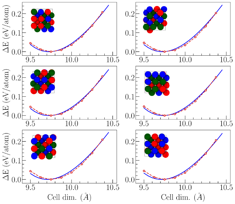
Figure 1: Equation of state calculations for six configurations. The red circles and blue lines display the high-fidelity DFT and low-fidelity SNAP results, respectively.

Fig. 1 displays the comparison of eight LF EOS calculations compared to the HF ones, at the equicomposition point. As detailed in Tranchida et al. Tranchida et al. (2020), about $\displaystyle 70\%$ of the training set of the SNAP potential contains equicomposition information. This explains the excellent agreement displayed on Fig. 1. Inferior agreement is expected when large departures from the equicomposition point are observed.

III Multi-fidelity Gaussian-process and multi-fidelity Bayesian optimization

In this section, we briefly review the formulation of GP, particularly the MF extension of the classical GP, and the relevant MF BO method Tran et al. (2020b, 2019a).

III.1 Gaussian Processes

Gaussian process regression is an efficient and flexible framework to approximate a response surface for a single-fidelity, single-objective function. We briefly summarize the GP theoretical formulation for the sake of completeness Shahriari et al. (2016). Let $\displaystyle\mathcal{D}=(\bm{x}_{i},y_{i})_{i=1:n}$ denote the dataset of $\displaystyle n$ observations with output $\displaystyle y$ and $\displaystyle d$-dimensional input $\displaystyle\bm{x}\in\mathcal{X}\subseteq\mathbb{R}^{d}$. A GP is a nonparametric model characterized by its prior mean function $\displaystyle\mu_{0}(\bm{x}):\mathcal{X}\to\mathbb{R}$ and a covariance function $\displaystyle k(\bm{x},\bm{x^{\prime}}):\mathcal{X}\times\mathcal{X}\to\mathbb{R}$. Assuming that the observations $\displaystyle\bm{f}=f_{1:n}$ are jointly Gaussian, and the observation $\displaystyle y$ is normally distributed given $\displaystyle\bm{f}$, i.e.

$$\bm{f}|\bm{x}\sim\mathcal{N}(\bm{m},\bm{K}),$$ (1)

$$\bm{y}|\bm{f},\sigma^{2}\sim\mathcal{N}(\bm{f},\sigma^{2}\bm{I}),$$ (2)

where $\displaystyle m_{i}:=\mu(\bm{x}_{i})$ and $\displaystyle K_{i,j}:=k(\bm{x}_{i},\bm{x}_{j})$.

The classical GP regression formulation assumes a stationary covariance matrix and only considers the weighted distance $\displaystyle r^{2}(\bm{x},\bm{x^{\prime}})=(\bm{x}-\bm{x^{\prime}})^{T}\Lambda(\bm{x}-\bm{x^{\prime}})$, where $\displaystyle\Lambda$ is a diagonal matrix of $\displaystyle d$ squared length scales $\displaystyle\theta_{i}^{2}$. Matérn kernels offer a broad class for stationary kernels, controlled by a smoothness parameter $\displaystyle\nu>0$ (cf. Section 4.2, Rasmussen (2006)), including the square-exponential ($\displaystyle\nu\to\infty$) and exponential $\displaystyle(\nu=1/2)$ kernels widely used in the literature. The $\displaystyle\nu=3/2$ Matérn kernel $\displaystyle k(\bm{x},\bm{x^{\prime}})=\theta_{0}^{2}\exp{(-\sqrt{3}r)}(1+\sqrt{3}r)$ is used in this work. At a known sampling point $\displaystyle\bm{x}\in\mathcal{X}$, the posterior mean $\displaystyle\mu(\bm{x})$ is calculated by

$$\mu(\bm{x})=\mu_{0}(\bm{x})+\bm{k}(\bm{x})^{T}(\bm{K}+\sigma^{2}\bm{I})^{-1}(\bm{y}-\bm{m}),$$ (3)

and the posterior variance $\displaystyle\sigma^{2}(\bm{x})$ is given by

$$\begin{array}[]{lll}\sigma^{2}(\bm{x})&=&k(\bm{x},\bm{x})\\ &&-\bm{k}(\bm{x})^{T}(\bm{K}+\sigma^{2}\bm{I})^{-1}\bm{k}(\bm{x}),\end{array}$$ (4)

where $\displaystyle\bm{k}(\bm{x})$ is a vector of covariance $\displaystyle\bm{k}(\bm{x})_{i}=k(\bm{x},\bm{x}_{i})$, $\displaystyle\sigma^{2}=\frac{1}{n}(\bm{y}-\mu_{0}(\bm{x}))^{T}\bm{K}^{-1}(\bm{y}-\mu_{0}(\bm{x}))$ is the intrinsic variance. To obtain the hyper-parameter $\displaystyle\theta=(\theta_{i})_{i=1:d}$, we maximize the log marginal likelihood, which is computed as

$$\begin{array}[]{lll}\log p(\bm{y}|\bm{x}_{1:n},\theta)&=&-\frac{1}{2}(\bm{y}-\bm{m})^{T}(\bm{K}^{\theta}+\sigma^{2}\bm{I})^{-1}(\bm{y}-\bm{m})\\ &&-\frac{1}{2}\log{|\bm{K}^{\theta}+\sigma^{2}\bm{I}|}-\frac{n}{2}\log{(2\pi)}.\end{array}$$ (5)

Here, $\displaystyle\bm{K}^{\theta}$ is emphasized to be strongly dependent on $\displaystyle\theta$.

III.2 Multi-fidelity Gaussian Processes

We assume that the prediction at highest level of fidelity, i.e. level $\displaystyle s$, can be written as an auto-regressive model Xiao et al. (2018),

$$f_{H}(\bm{x})=\rho f_{L}(\bm{x})+\delta(\bm{x}),$$ (6)

where $\displaystyle f_{H}(\bm{x})$ and $\displaystyle f_{L}(\bm{x})$ denote the high- and low-fidelity predictions, respectively, $\displaystyle\rho$ is the scaling factor, and $\displaystyle\delta(\bm{x})$ is the discrepancy between the high- and low-fidelity model. The dataset $\displaystyle\mathcal{D}$ is divided into $\displaystyle\mathcal{D}_{L}=(\bm{x}_{i},y_{i})_{i=1:n_{L}}$ and $\displaystyle\mathcal{D}_{H}=(\bm{x}_{i},y_{i})_{i=1:n_{H}}$, corresponding to low-fidelity and high-fidelity datasets, respectively. Our multi-fidelity formulation is closely related to Couckuyt et al.  Couckuyt et al. (2012, 2013, 2014) and Forrester et al.  Forrester et al. (2007). Following the auto-regressive scheme described in Equation 6, the main idea of MFGP in two levels of fidelity is to model $\displaystyle f_{L}$ as the first GP and the discrepancy $\displaystyle\delta(\bm{x})$ as the second GP, before fusing both of them together.

In the MFGP, the covariance matrix $\displaystyle\tilde{K}$ is computed as

$$\tilde{\bm{K}}=\begin{pmatrix}\sigma_{L}^{2}\bm{K}_{L}(\bm{x}_{L},\bm{x}_{L})&\rho\sigma_{L}^{2}\bm{K}_{L}(\bm{x}_{L},\bm{x}_{H})\\ \rho\sigma_{L}^{2}\bm{K}_{L}(\bm{x}_{H},\bm{x}_{L})&~{}~{}\rho^{2}\sigma_{L}^{2}\bm{K}_{L}(\bm{x}_{H},\bm{x}_{H})+\sigma_{d}^{2}\bm{K}_{D}(\bm{x}_{H},\bm{x}_{H})\end{pmatrix}.$$ (7)

At the high-fidelity level, the posterior mean $\displaystyle\mu(\bm{x})$ and the posterior variance $\displaystyle\sigma^{2}(\bm{x})$ are computed, respectively, as

$$\begin{array}[]{lll}\mu(\bm{x})&=&\mu_{0}(\bm{x})+\tilde{\bm{k}}(\bm{x})^{T}(\tilde{\bm{K}}+\sigma^{2}\bm{I})^{-1}(\tilde{\bm{y}}-\tilde{\bm{m}}),\\ \sigma^{2}(\bm{x})&=&\rho^{2}\sigma_{L}^{2}(\bm{x})+\sigma_{d}^{2}(\bm{x})\\ &&-\tilde{\bm{k}}(\bm{x})(\tilde{\bm{K}}+\sigma^{2}\bm{I})^{-1}\tilde{\bm{k}}(\bm{x}),\\ \end{array}$$ (8)

where

$$\begin{array}[]{lll}\mu_{H}(\bm{x})&=&\rho\mu_{L}(\bm{x})+\mu_{d}(\bm{x}),\\ \sigma_{L}^{2}(\bm{x})&=&k_{L}(\bm{x},\bm{x}),\\ \sigma_{d}(\bm{x})&=&k_{d}(\bm{x},\bm{x}),\\ \tilde{\bm{y}}&=&\begin{pmatrix}\bm{y}_{L}^{T}\\ \bm{y}_{H}^{T}\end{pmatrix}=\begin{pmatrix}\left(y_{1,L},\dots,y_{n_{L},_{L}}\right)^{T}\\ \left(y_{1,H},\dots,y_{n_{H},_{H}}\right)^{T}\end{pmatrix},\\ \tilde{\bm{m}}&=&\begin{pmatrix}\bm{\mu}_{L}\\ \bm{\mu}_{H}\end{pmatrix}\\ &=&\begin{pmatrix}\left(\mu_{L}(\bm{x}_{1,L}),\dots,\mu_{L}(\bm{x}^{n_{L},L})\right)^{T}\\ \left(\mu_{H}(\bm{x}_{1,H}),\dots,\mu_{H}(\bm{x}^{n_{H},H})\right)^{T}\end{pmatrix},\\ \tilde{\bm{k}}(\bm{x})&=&\begin{pmatrix}\rho\bm{k}_{L}(\bm{x})\\ \bm{k}_{H}(\bm{x})\end{pmatrix}\\ &=&\begin{pmatrix}\left(\rho k_{L}(\bm{x},\bm{x}_{1,L}),\dots,\rho k_{L}(\bm{x},\bm{x}_{n_{L},L})\right)^{T}\\ \left(k_{H}(\bm{x},\bm{x}_{1,H}),\dots,k_{H}(\bm{x},\bm{x}_{n_{H},H})\right)^{T}\end{pmatrix}\\ k_{H}(\bm{x},\bm{x^{\prime}})&=&\rho^{2}k_{L}(\bm{x},\bm{x^{\prime}})+k_{d}(\bm{x},\bm{x^{\prime}}).\\ \end{array}$$ (9)

$\displaystyle\bm{x}_{i,L}$ and $\displaystyle\bm{x}_{i,H}$ denote the $\displaystyle i^{\text{th}}$ inputs at the low- and high-fidelity levels, respectively. $\displaystyle y_{i,L}$ and $\displaystyle y_{i,H}$ denote the $\displaystyle i^{\text{th}}$ observations at the low- and high-fidelity levels, respectively. The hyper-parameters in $\displaystyle\tilde{\theta}=(\theta_{L},\theta_{H})$ in $\displaystyle k_{L}(\cdot,\cdot)$ and $\displaystyle k_{D}(\cdot,\cdot)$ can be obtained by maximizing the log marginal likelihood as

$$\begin{array}[]{lll}&&\log p(\tilde{\bm{y}}|\bm{x}_{1:n_{L}},\bm{x}_{1:n_{H}},\tilde{\theta})\\ &=&-\frac{1}{2}(\tilde{\bm{y}}-\tilde{\bm{m}})^{T}(\tilde{\bm{K}}^{\tilde{\theta}}+\sigma^{2}\bm{I})^{-1}(\tilde{\bm{y}}-\tilde{\bm{m}})\\ &&-\frac{1}{2}\log{|\tilde{\bm{K}}^{\tilde{\theta}}+\sigma^{2}\bm{I}|}-\frac{n_{H}+n_{L}}{2}\log{(2\pi)}.\end{array}$$ (10)

For further details, readers are referred to previous work in literature Couckuyt et al. (2013); Xiao et al. (2018); Yang et al. (2020).

III.3 Multi-fidelity Bayesian Optimization

In the traditional BO method, the next sampling location is determined by maximizing an acquisition function, i.e.,

$$\bm{x}^{*}=\operatorname*{argmax}_{\bm{x}\in\mathcal{X}}\ a(\bm{x}),$$ (11)

where $\displaystyle a(\bm{x})$ denotes the acquisition function and $\displaystyle\bm{x}^{*}$ is the next sampling location. The acquisition function is deeply connected to an underlying utility function, which corresponds to a reward scheme for performance of the new sampling point relative to previous samples. There are three acquisition functions that are widely used: the probability of improvement (PI), the expected improvement (EI), and the upper-confident bounds (UCB), but other forms also exist.

The UCB acquisition function Srinivas et al. (2009, 2012); Daniel et al. (2014) is defined as

$$a_{\text{UCB}}(\bm{x};\{\bm{x}_{i},y_{i}\}_{i=1}^{n},\theta)=\\ \mu(\bm{x};\{\bm{x}_{i},y_{i}\}_{i=1}^{n},\theta)+\kappa\sigma(\bm{x};\{\bm{x}_{i},y_{i}\}_{i=1}^{n},\theta),$$ (12)

where $\displaystyle\kappa$ is a hyper-parameter describing the acquisition exploitation-exploration balance. We adopt the $\displaystyle\kappa$ computation from Daniel et al. Daniel et al. (2014), which is based on Srinivas et al. Srinivas et al. (2009, 2012), instead of fixing $\displaystyle\kappa$ as a constant.

Regarding the fidelity selection criteria, we adopt the approach developed in Tran et al. (2020b) by choosing level $\displaystyle t^{*}$ such that

$$t^{*}=\operatorname*{argmin}_{t}\left(C_{t}\int_{\mathcal{X}}\sigma^{2}(\bm{x})d\bm{x}\right),$$ (13)

where $\displaystyle C_{t}$ is the computational cost at level $\displaystyle t$, $\displaystyle t$ can be low- or high-fidelity level. The term $\displaystyle\int_{\mathcal{X}}\sigma^{2}(\bm{x})d\bm{x}$ is sometimes referred to as the integrated mean square error, as opposed to the conventional mean square error $\displaystyle\sigma^{2}(\bm{x})$, to reduce the number of sampling points on the boundary of $\displaystyle\mathcal{X}$ for further efficiency improvement. To facilitate information at the high-fidelity level when the computational cost are comparable, we impose a hard condition that if $\displaystyle C_{L}n_{L}\geq C_{H}n_{H}$, meaning that some of the computational budget for building the low-fidelity dataset $\displaystyle\mathcal{D}_{L}$ could be traded for building the high-fidelity dataset $\displaystyle\mathcal{D}_{H}$, then the high-fidelity is chosen.

IV Results

IV.1 Fusing low- and high-fidelity bulk modulus predictions

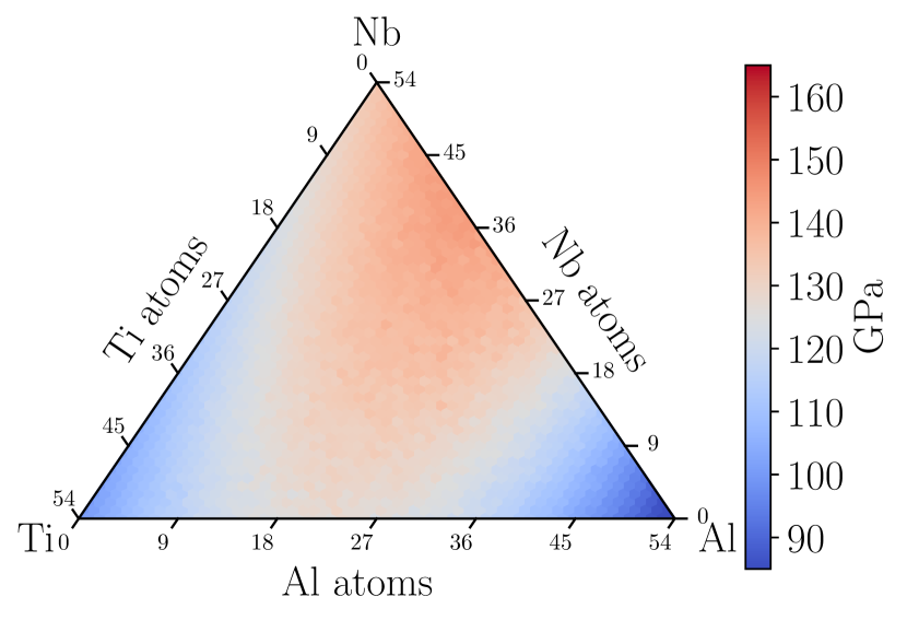
(a) Low-fidelity.

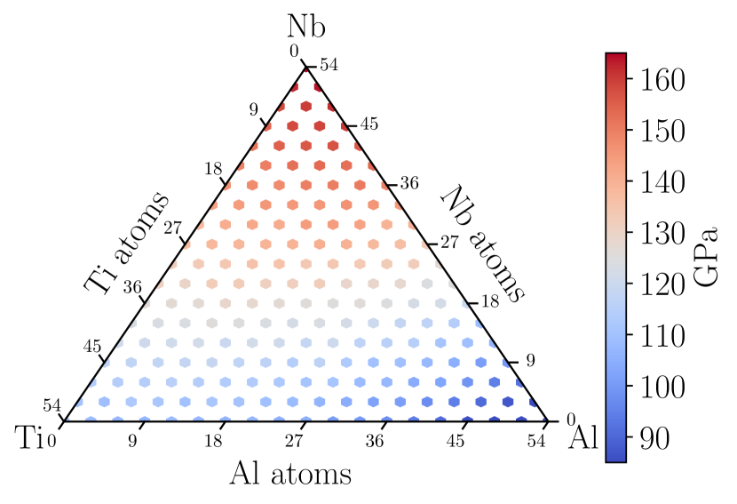
(b) High-fidelity.

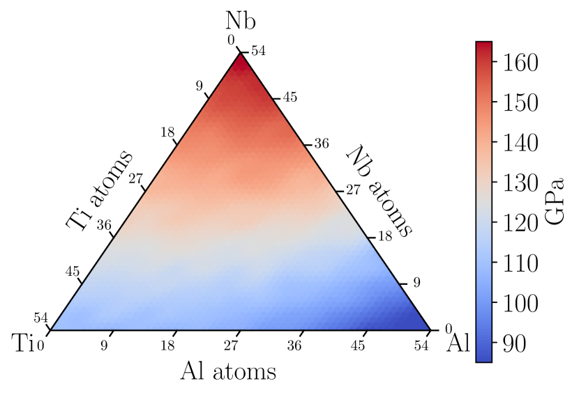
(c) Multi-fidelity.

Figure 2: Low-fidelity (SNAP potential – Figure 2(a)) and high-fidelity (DFT – Figure 2(b)) calculated values of bulk modulus for AlNbTi ternary compositions, as well as multi-fidelity (SNAP/DFT – Figure 2(c)) predictions.

As explained in section II.1 and II.2, 190 HF and 1540 LF calculations of bulk modulus at different compositions were performed to build the dataset. Figure 2 displays the LF (Fig. 2(a)) and HF (Fig. 2(b)) data sets, as well as the MF predictions using the MFGP approach (Fig. 2(c)). As can be seen by comparing Fig. 2(b) and Fig. 2(c), starting from a sparse HF ternary composition map, the MFGP approach is able to leverage the LF-HF correlations to produce a high-resolution diagram predicting the composition dependence of the bulk modulus with an accuracy almost equal to DFT.

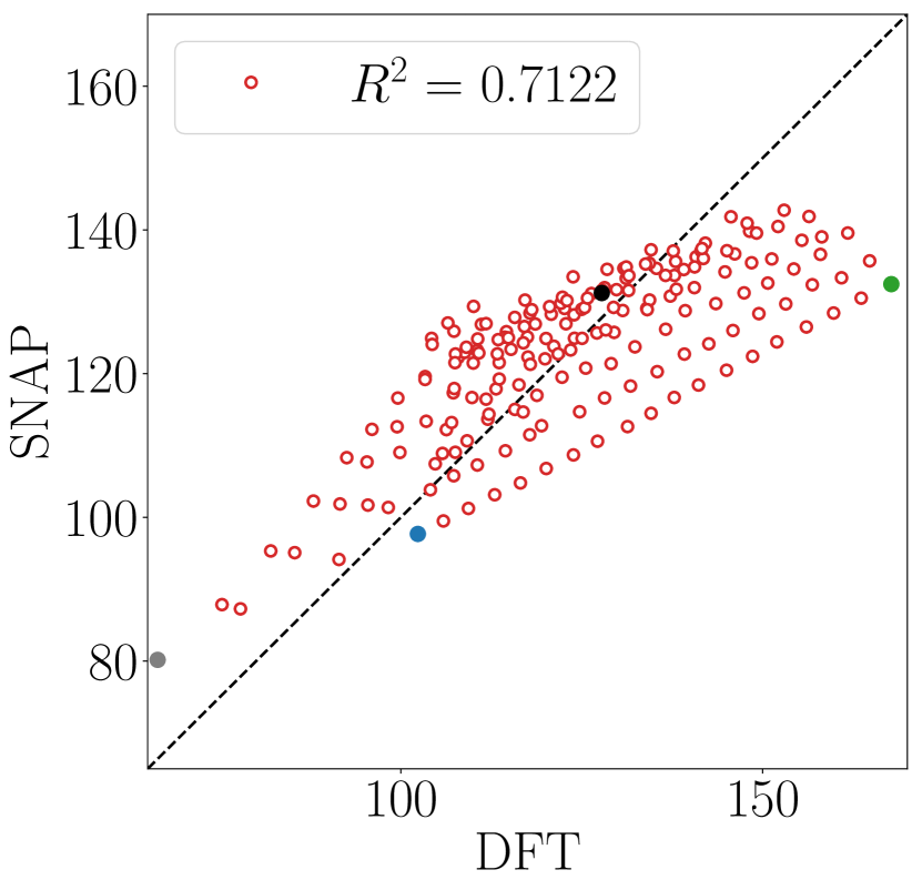
(a) SNAP

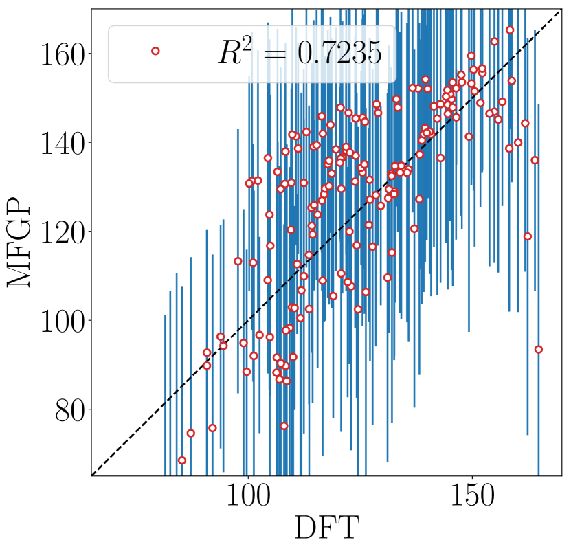
(b) MFGP-10

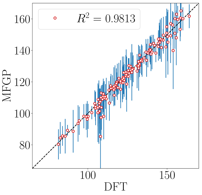
(c) MFGP-30

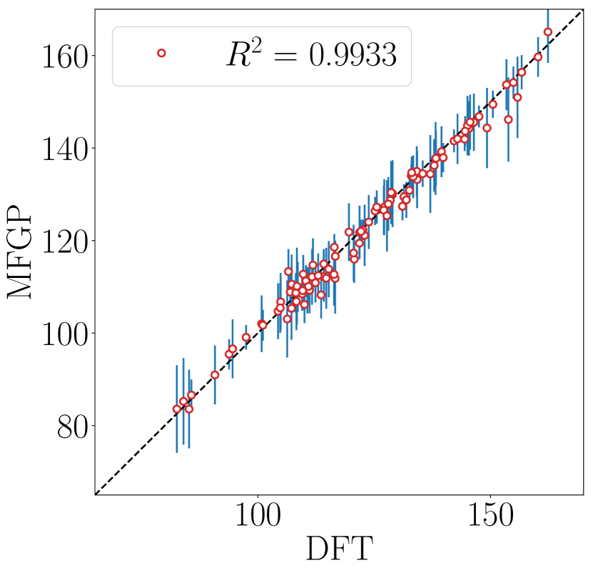
(d) MFGP-50

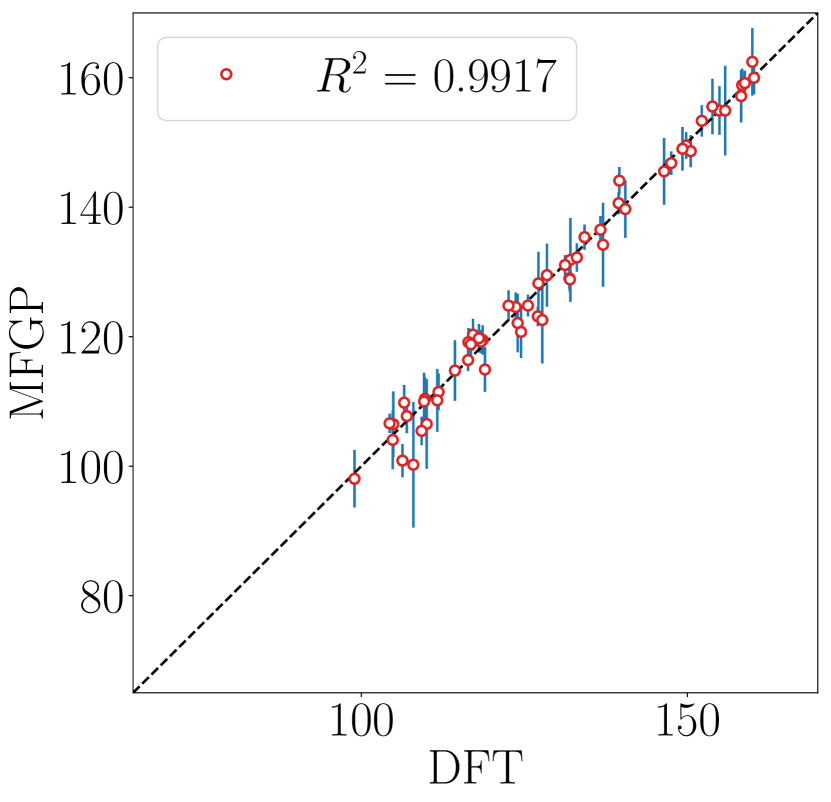
(e) MFGP-70

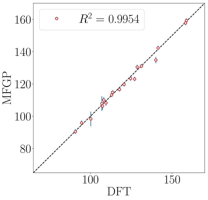
(f) MFGP-90

Figure 3: Comparison of the low-fidelity (SNAP, Figure 3(a)) and multi-fidelity (MFGP, Figs. 3(b)- 3(f)) models against the high-fidelity model (DFT) estimates of bulk modulus (GPa). For the SNAP model, estimates for all the AlNbTi ternary compositions in Figure 2(b) are shown. Pure aluminum, pure niobium, pure titanium and the equicomposition point for the grey, green, blue and black dots, respectively. For each MFGP models, the random fraction of the DFT data used in training is indicated in the subcaption (MFGP-N meaning that N % of the HF dataset was used to train the corresponding MFGP model), with remaining DFT points shown in the figure. Vertical blue bars indicate the associated uncertainty quantification $\displaystyle\mu\pm 1.0\sigma$. The legends indicate the squared correlation coefficients $\displaystyle R^{2}$.

Fig. 3 assesses the accuracy evolution of the approach by displaying the numerical predictions of the SNAP ML-IAP and of the MFGP results at various sizes of training datasets, with respect to the DFT predictions. For the MFGP, it also provides us with a measure of uncertainty quantification by displaying the posterior Gaussian process prediction of $\displaystyle\mu\pm 1.0\sigma$ (vertical bars).

Across the full ternary composition range, the SNAP potential predictions correlate with the DFT results with $\displaystyle R^{2}=0.7122$ (Fig. 3(a)). Fig. 3(a) highlights the SNAP bulk modulus results of the pure element and equicomposition points. As explained in section II.2, about 70% of the training set of the SNAP potential consisted in data at the equicomposition point, which explains the very good agreement observed for that particular composition. Figs. 3(b)-3(f) display the rapid convergence of the MFGP towards the DFT results with an increasing training dataset size. The dataset size was varied by randomly choosing a fraction of the full HF dataset. The remaining HF points were used as a testing dataset and are plotted in Figs 3(b)-3(f).

With a 10% training dataset (19 LF and 19 HF data points, Fig. 3(b)) to train the MFGP model, the MFGP performs on a par with the LF SNAP model ($\displaystyle R^{2}=0.7235$). Increasing the training dataset to 30% (57 LF and 57 HF data points, Fig. 3(c)) and 50% (95 LF and 95 HF data points, Fig. 3(d)) considerably improved the accuracy of the prediction ($\displaystyle R^{2}=0.9813$ and $\displaystyle R^{2}=0.9933$, respectively) and reduced the uncertainty. Additional increases to 70% (133 LF and 133 HF data points, Fig. 3(e)) and 90% (171 LF and 171 HF data points, Fig. 3(f)) of the training dataset do not significantly improve the predictions (i.e. the posterior mean) as there is almost no change in the correlation coefficients $\displaystyle R^{2}$, but increase the confidence in those predictions by reducing the uncertainty (i.e. the posterior variance).

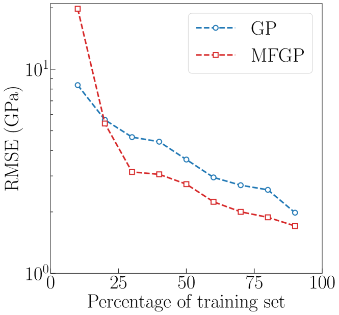
Figure 4: Convergence of the GP (single-fidelity) and MFGP (multi-fidelity) RMSE of bulk modulus prediction as a function of the amount of training data used. For each point, the HF training and testing training data are the same.

In order to probe the improvement in learning efficiency obtained from the use of the MFGP model, we generated learning curves for both MFGP and single-fidelity GP. Fig. 4 compares the bulk modulus root mean-squared error (RMSE) convergence of the MFGP to a single-fidelity GP model. Once a sufficient amount of data is added to the training set, the RMSE of the MFGP model is consistently below that of the single-fidelity GP. This demonstrates the improved learning obtained by adding a level of fidelity to the model.

A computational cost assessment and comparison of the two levels of fidelity and of the MFGP model was also performed. For consistency, all calculations were performed on Sandia’s Solo cluster consisting of dual-socket Intel Xeon E5-2695 (Broadwell) CPUs with 36 cores per node, and an Intel Omnipath interconnect. Each HF and LF bulk modulus prediction is obtained in computation times of approximately 4.1 and 1.83$\displaystyle\times 10^{-6}$ hours, on 2 and 1 Solo nodes, respectively. This leads to relative speeds of 297.6 hours per core for the HF model, and of 6.6 $\displaystyle\times 10^{-5}$ hours per core for the LF model. In comparison, the MFGP model performs a bulk modulus prediction with a relative speed of 1.95$\displaystyle\times 10^{-7}$ hours per core (approximately 1.95$\displaystyle\times 10^{-7}$ hours to perform one bulk modulus prediction on one core). The relative speed of each different model (HF, LF and MFGP) differs by orders of magnitude. Once trained, the MFGP model allows to perform predictions with accuracy comparable to the HF calculations for an almost negligible computational cost.

IV.2 Multi-fidelity Bayesian optimization of bulk modulus

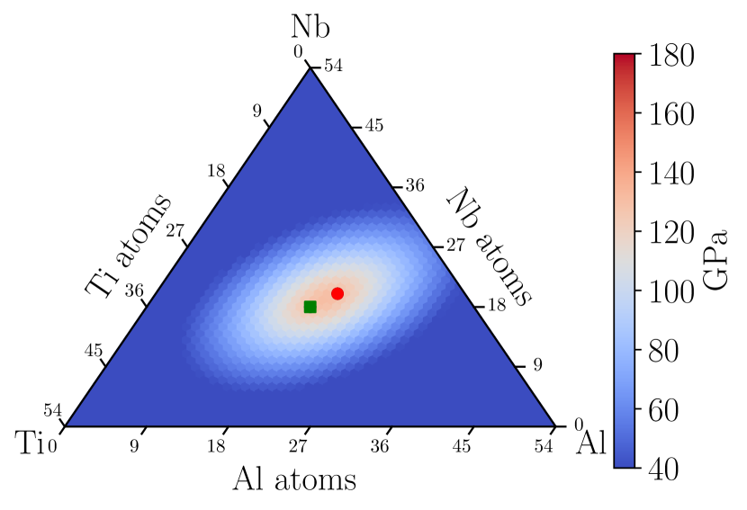
(a) Iteration 4: 2 LF + 2 HF.

(b) Iteration 24: 21 LF + 3 HF.

(c) Iteration 35: 31 LF + 4 HF.

(d) Iteration 130: 116 LF + 14 HF.

Figure 5: Progression of the multi-fidelity Bayesian optimization (MF BO) for bulk modulus in the ternary composition space of AlNbTi alloys. The color map indicates the MFGP predictions at iterations 4, 24, 35, and 130. The red dot indicates the best HF data point evaluated so far, while the green squares indicate the other HF data points and the green black dots indicate LF data points. At iteration 35, MF BO finds the global optimum near the niobium vertex after evaluating only 4 HF points.

We demonstrate the application MF BO for practical materials design by searching for the chemical composition optimizing the QoI across the ternary AlNbTi composition range, and using the MFGP framework to couple the SNAP and DFT predictions. The computational cost ratio between DFT and MD simulations is set to 10.0, and the UCB acquisition function is used.

The concept of using the acquisition function described in Section III.3 allows the MF BO to sequentially sample at the most informative point. Four sampling points, including 2 LF and 2 HF points around the equicomposition point, are used to build the initial MFGP, as shown in Fig. 5(a). At iteration 24, the MF BO queries another HF evaluation (Fig. 5(b)) in the vicinity of the global maximum given by the LF predictions, as shown in Fig. 2(a), and corrects itself after obtaining the corresponding HF sampling value. The global maximum is obtained at iteration 35 (Fig. 5(c)) after only four HF and 31 LF evaluations.

V Conclusions

This work presented and applied a scale-bridging MFGP framework fusing information from DFT and MD calculations performed with a SNAP ML-IAP. Equation-of-state (EOS) calculations were performed with DFT and the SNAP potential across the full AlNbTi ternary composition range. The EOS data allowed us to extract 190 high- and 1540 low-fidelity predictions of the QoI, the bulk modulus. This full dataset (HF + LF predictions) is used as a training set. The HF configurations are also used as reference values to probe the validity of our approach (testing set).

The MFGP framework is then applied to this dataset to build a MF model. Its efficiency is demonstrated through the construction of a high-resolution and highly accurate ternary composition diagram for the QoI using only 50% of the HF data points (corresponding to 95 EOS evaluations performed with DFT) with an excellent correlation coefficient of $\displaystyle R^{2}=0.9933$ and low prediction uncertainty. Additional increase of the training dataset size allowed even lower prediction uncertainty.

By leveraging LF-HF correlations, our framework drastically reduces the amount of expensive first principles calculations necessary to obtain a dense and highly accurate ternary composition diagram for the property of interest. An MF BO algorithm is finally presented and tested by performing an optimization of the QoI. After only 4 HF and 31 LF evaluations, the MF BO algorithm was able to locate the QoI optimum value across the composition space. Performed on the fly, the computational cost associated with materials property optimization and design would be drastically reduced.

For the QoI we used in this study, the optimization problem was trivial, as pure niobium has the highest value of bulk modulus across the AlNbTi composition space. However, reapplying the same framework to a different material composition space and QoI is straightforward. In future work, our framework will be extended to perform multi-objective Tran et al. (2020c); Shu et al. (2020), constrained mixed-integer Tran et al. (2019b) MF calculations, allowing to search for optimum compromises between different materials properties in an asynchronously parallel manner Tran et al. (2019c, 2020d).

Our results demonstrated the efficiency of our a MFGP framework to fuse in the predictions and therefore bridge the gap between two of the most commonly employed atomistic simulation approaches (DFT and molecular dynamics), each of them acting at very different length and time scales. The same methodology remains valid for different scales, and could be leveraged to build materials modelling road-maps van der Giessen et al. (2020) by understanding the existing correlations between atomistic methods Bulatov et al. (1998); Tranchida et al. (2018a); Zepeda-Ruiz et al. (2017) and associated higher scale coarse-grained Tranchida et al. (2018b) or continuum numerical models Arsenlis et al. (2007); Roters et al. (2010).

Data Availability

The data that support the findings of this study are available from the corresponding authors upon reasonable request.

References

- Gubaev et al. (2019) K. Gubaev, E. V. Podryabinkin, G. L. Hart, and A. V. Shapeev, Computational Materials Science 156, 148 (2019).
- Kostiuchenko et al. (2019) T. Kostiuchenko, F. Körmann, J. Neugebauer, and A. Shapeev, npj Computational Materials 5, 1 (2019).
- Wen et al. (2019) C. Wen, Y. Zhang, C. Wang, D. Xue, Y. Bai, S. Antonov, L. Dai, T. Lookman, and Y. Su, Acta Materialia 170, 109 (2019).
- Guerra et al. (1998) C. F. Guerra, J. Snijders, G. t. te Velde, and E. J. Baerends, Theoretical Chemistry Accounts 99, 391 (1998).
- Bartók et al. (2010) A. P. Bartók, M. C. Payne, R. Kondor, and G. Csányi, Physical review letters 104, 136403 (2010).
- Zuo et al. (2020) Y. Zuo, C. Chen, X. Li, Z. Deng, Y. Chen, J. Behler, G. Csányi, A. V. Shapeev, A. P. Thompson, M. A. Wood, et al., The Journal of Physical Chemistry A 124, 731 (2020).
- Chen et al. (2017) C. Chen, Z. Deng, R. Tran, H. Tang, I.-H. Chu, and S. P. Ong, Physical Review Materials 1, 043603 (2017).
- Wood et al. (2019) M. A. Wood, M. A. Cusentino, B. D. Wirth, and A. P. Thompson, Physical Review B 99, 184305 (2019).
- Batra and Sankaranarayanan (2020) R. Batra and S. Sankaranarayanan, arXiv preprint arXiv:2004.00232 (2020).
- Pilania et al. (2017) G. Pilania, J. E. Gubernatis, and T. Lookman, Computational Materials Science 129, 156 (2017).
- Acar (2018) P. Acar, Integrating Materials and Manufacturing Innovation 7, 186 (2018).
- Sun et al. (2010) G. Sun, G. Li, M. Stone, and Q. Li, Computational Materials Science 49, 500 (2010).
- Razi et al. (2018) M. Razi, A. Narayan, R. Kirby, and D. Bedrov, Computational Materials Science 152, 125 (2018).
- Chen et al. (2020) C. Chen, Y. Zuo, W. Ye, X. Li, and S. P. Ong, arXiv preprint arXiv:2005.04338 (2020).
- Ramprasad et al. (2017) R. Ramprasad, R. Batra, G. Pilania, A. Mannodi-Kanakkithodi, and C. Kim, npj Computational Materials 3, 1 (2017).
- Xue et al. (2016) D. Xue, P. V. Balachandran, J. Hogden, J. Theiler, D. Xue, and T. Lookman, Nature communications 7, 1 (2016).
- Mannodi-Kanakkithodi et al. (2016) A. Mannodi-Kanakkithodi, G. Pilania, T. D. Huan, T. Lookman, and R. Ramprasad, Scientific reports 6, 20952 (2016).
- Patra et al. (2020) A. Patra, R. Batra, A. Chandrasekaran, C. Kim, T. D. Huan, and R. Ramprasad, Computational Materials Science 172, 109286 (2020).
- Tran et al. (2020a) A. Tran, D. Liu, L. He-Bitoun, and Y. Wang, in Uncertainty Quantification in Multiscale Materials Modeling (Elsevier, 2020).
- Tran et al. (2018) A. Tran, L. He, and Y. Wang, ASCE-ASME Journal of Risk and Uncertainty in Engineering Systems, Part B: Mechanical Engineering 4, 011006 (2018).
- Koistinen et al. (2019) O.-P. Koistinen, V. Asgeirsson, A. Vehtari, and H. Jónsson, Journal of Chemical Theory and Computation (2019).
- Razi et al. (2020) M. Razi, A. Narayan, R. Kirby, and D. Bedrov, Computational Materials Science 176, 109518 (2020).
- Tran et al. (2019a) A. Tran, T. Wildey, and S. McCann, in Proceedings of the ASME 2019 IDETC/CIE, International Design Engineering Technical Conferences and Computers and Information in Engineering Conference, Vol. Volume 1: 39th Computers and Information in Engineering Conference (American Society of Mechanical Engineers, 2019) v001T02A073.
- Tran et al. (2020b) A. Tran, T. Wildey, and S. McCann, Journal of Computing and Information Science in Engineering 20, 1 (2020b).
- Thompson et al. (2015) A. P. Thompson, L. P. Swiler, C. R. Trott, S. M. Foiles, and G. J. Tucker, Journal of Computational Physics 285, 316 (2015).
- Mattsson et al. (2004) A. E. Mattsson, P. A. Schultz, M. P. Desjarlais, T. R. Mattsson, and K. Leung, Modelling and Simulation in Materials Science and Engineering 13, R1 (2004).
- Giannozzi et al. (2009) P. Giannozzi, S. Baroni, N. Bonini, M. Calandra, R. Car, C. Cavazzoni, D. Ceresoli, G. L. Chiarotti, M. Cococcioni, I. Dabo, et al., Journal of physics: Condensed matter 21, 395502 (2009).
- Giannozzi et al. (2017) P. Giannozzi, O. Andreussi, T. Brumme, O. Bunau, M. B. Nardelli, M. Calandra, R. Car, C. Cavazzoni, D. Ceresoli, M. Cococcioni, et al., Journal of Physics: Condensed Matter 29, 465901 (2017).
- Perdew et al. (1996) J. P. Perdew, K. Burke, and M. Ernzerhof, Physical review letters 77, 3865 (1996).
- Tran et al. (2016) F. Tran, J. Stelzl, and P. Blaha, The Journal of chemical physics 144, 204120 (2016).
- Saal et al. (2013) J. E. Saal, S. Kirklin, M. Aykol, B. Meredig, and C. Wolverton, Jom 65, 1501 (2013).
- Tranchida et al. (2020) J. Tranchida, P. A. Schultz, A. Tran, M. E. Chandross, and A. P. Thompson, Modelling and Simulation in Materials Science and Engineering 13 (2020), to be published.
- Birch (1978) F. Birch, Journal of Geophysical Research: Solid Earth 83, 1257 (1978).
- Murnaghan (1937) F. D. Murnaghan, American Journal of Mathematics 59, 235 (1937).
- Plimpton (1995) S. Plimpton, Journal of Computational Physics 117, 1 (1995).
- Shahriari et al. (2016) B. Shahriari, K. Swersky, Z. Wang, R. P. Adams, and N. de Freitas, Proceedings of the IEEE 104, 148 (2016).
- Rasmussen (2006) C. E. Rasmussen, Gaussian processes in machine learning (MIT Press, 2006).
- Xiao et al. (2018) M. Xiao, G. Zhang, P. Breitkopf, P. Villon, and W. Zhang, Applied Mathematics and Computation 323, 120 (2018).
- Couckuyt et al. (2012) I. Couckuyt, A. Forrester, D. Gorissen, F. De Turck, and T. Dhaene, Advances in Engineering Software 49, 1 (2012).
- Couckuyt et al. (2013) I. Couckuyt, T. Dhaene, and P. Demeester, Universiteit Gent , 3 (2013).
- Couckuyt et al. (2014) I. Couckuyt, T. Dhaene, and P. Demeester, The Journal of Machine Learning Research 15, 3183 (2014).
- Forrester et al. (2007) A. I. Forrester, A. Sóbester, and A. J. Keane, Proceedings of the Royal Society of London A: mathematical, physical and engineering sciences 463, 3251 (2007).
- Yang et al. (2020) X. Yang, X. Zhu, and J. Li, SIAM Journal on Scientific Computing 42, A220 (2020).
- Srinivas et al. (2009) N. Srinivas, A. Krause, S. M. Kakade, and M. Seeger, arXiv preprint arXiv:0912.3995 (2009).
- Srinivas et al. (2012) N. Srinivas, A. Krause, S. M. Kakade, and M. W. Seeger, IEEE Transactions on Information Theory 58, 3250 (2012).
- Daniel et al. (2014) C. Daniel, M. Viering, J. Metz, O. Kroemer, and J. Peters, in Robotics: Science and Systems (2014).
- Tran et al. (2020c) A. Tran, M. Eldred, Y. Wang, and S. McCann, in Proceedings of the ASME 2020 IDETC/CIE, International Design Engineering Technical Conferences and Computers and Information in Engineering Conference, Vol. Volume 1: 40th Computers and Information in Engineering Conference (American Society of Mechanical Engineers, 2020).
- Shu et al. (2020) L. Shu, P. Jiang, X. Shao, and Y. Wang, Journal of Mechanical Design 127, 1 (2020).
- Tran et al. (2019b) A. Tran, M. Tran, and Y. Wang, Structural and Multidisciplinary Optimization , 1 (2019b).
- Tran et al. (2019c) A. Tran, J. Sun, J. M. Furlan, K. V. Pagalthivarthi, R. J. Visintainer, and Y. Wang, Computer Methods in Applied Mechanics and Engineering 347, 827 (2019c).
- Tran et al. (2020d) A. Tran, J. A. Mitchell, L. P. Swiler, and T. Wildey, Acta Materialia 194, 80 (2020d).
- van der Giessen et al. (2020) E. van der Giessen, P. A. Schultz, N. Bertin, V. V. Bulatov, W. Cai, G. Csányi, S. M. Foiles, M. Geers, C. González, M. Hütter, et al., Modelling and Simulation in Materials Science and Engineering 28, 043001 (2020).
- Bulatov et al. (1998) V. Bulatov, F. F. Abraham, L. Kubin, B. Devincre, and S. Yip, Nature 391, 669 (1998).
- Tranchida et al. (2018a) J. Tranchida, S. Plimpton, P. Thibaudeau, and A. P. Thompson, Journal of Computational Physics 372, 406 (2018a).
- Zepeda-Ruiz et al. (2017) L. A. Zepeda-Ruiz, A. Stukowski, T. Oppelstrup, and V. V. Bulatov, Nature 550, 492 (2017).
- Tranchida et al. (2018b) J. Tranchida, P. Thibaudeau, and S. Nicolis, Physical Review E 98, 042101 (2018b).
- Arsenlis et al. (2007) A. Arsenlis, W. Cai, M. Tang, M. Rhee, T. Oppelstrup, G. Hommes, T. G. Pierce, and V. V. Bulatov, Modelling and Simulation in Materials Science and Engineering 15, 553 (2007).
- Roters et al. (2010) F. Roters, P. Eisenlohr, L. Hantcherli, D. D. Tjahjanto, T. R. Bieler, and D. Raabe, Acta Materialia 58, 1152 (2010).