Abstract

This paper presents a windowed Green function (WGF) method for the numerical solution of problems of elastic scattering by “locally-rough surfaces” (i.e., local perturbations of a half space), under either Dirichlet or Neumann boundary conditions, and in both two and three spatial dimensions. The proposed WGF method relies on an integral-equation formulation based on the free-space Green function, together with smooth operator windowing (based on a “slow-rise” windowing function) and efficient high-order singular-integration methods. The approach avoids the evaluation of the expensive layer Green function for elastic problems on a half-space, and it yields uniformly fast convergence for all incident angles. Numerical experiments for both two and three dimensional problems are presented, demonstrating the accuracy and super-algebraically fast convergence of the proposed method as the window-size grows. Keywords: Elastic wave, half-space, windowed Green function, boundary integral equation

1 Introduction

In view of their great importance in diverse areas of applications, the problems of scattering by unbounded rough-surfaces, including scattering of acoustic, electromagnetic, and elastic waves, have attracted the interest of physicists, engineers, and mathematicians for many years. Specifically, simulations concerning elastic half-space problems (in which material interfaces are everywhere planar, except for bounded regions which may contain arbitrarily complex structures) play essential roles in the investigation of earthquakes, non-destructive testing of materials, and energy production from natural gas and geothermal sources [1, 3, 36]. This paper introduces an efficient high-order integral solver for problems of this type. More precisely, this paper presents an efficient and accurate methodology, based on surface integral equations over the material interfaces, for the problem of elastic wave scattering over a half-space [4, 5, 6, 26, 27]. In particular, the method is applicable to configurations in which the scattering boundary is a combination of an unbounded flat surface and local (bounded) non-planar surface perturbations and/or bounded elastic scatterers. Unlike the volumetric discretization methods for these problems, the boundary integral equation (BIE) approach [29, 33] only requires discretization of regions of lower dimensionality, and it automatically enforces the radiation condition at infinity. In conjunction with adequate acceleration techniques (see e.g. [14, 18, 31]) for the associated matrix-vector products and Krylov-subspace linear algebra solver such as GMRES, the BIE method can provide fast, high-order solvers even for problems of high frequency.

Two main integral equation approaches have been used for scattering problems on a half-space. One is based on the layer Green function (LGF) [4, 20, 24, 25]—which automatically enforces the relevant boundary conditions on the unbounded flat surfaces and thus reduces the scattering problems to integral equations on the defects. It should be pointed out that the Dirichlet and Neumann cases, for which the layer Green function is trivially calculated in the acoustic case, require Fourier-transform based layer Green function in the elastic case. A second approach relies on integral equations imposed on the complete unbounded surface [11, 23, 21, 35]. The potential benefits of the second approach arise from its use of the free-space Green-function kernel, whose evaluation cost is much lower, by orders of magnitude, than the LGF evaluation cost—since evaluation of a single value of the LGF requires computation of challenging Fourier integrals containing highly-oscillatory integrands over infinite integration intervals; see e.g. [4, Eq. (2.27)] and [20, Eq. (26)].

The integral equations based on the free-space Green function, on the other hand, are posed on the complete unbounded interface, and they therefore require, for computational purposes, use of a domain-truncation strategy of some sort—which raises questions with regard to selection of suitable truncation radii and the potentially large number of required unknowns [2, 19]. For the elastic scattering problems in a half-space, a direct-truncation approach is discussed in [18, 19, 28] (in which, significantly, only normal-incidence problems are considered). The examples considered in these papers suggest that a truncation radius equal to three to five times the radius of the surface irregularity yields acceptable accuracy for normal-incidence problems. However, as illustrated in Section 3.1 for a related approach, this truncation strategy requires, for a given accuracy, use of larger and larger truncated domains as the incidence angles depart from normal, with required inclusion of planar sections that grow beyond all finite bounds as the incidence angle approaches grazing.

The present paper proposes a novel truncation approach, called the windowed Green function (WGF) method, for the problem of elastic scattering on a half-space. The WGF method has previously been found effective in the contexts of acoustic and electromagnetic scattering by periodic structures [10, 16, 32], multiply-layered media [11, 15, 35], waveguide structures [13] and long-range volumetric propagation [22]. On the basis of certain “slow-rise” windowing functions $\widetilde{w}_{A}$, the WGF method we propose here truncates the original integral equations over unbounded surfaces to integration domains that include the surface defects and appropriate portions of the flat interfaces. As for the direct-truncation method, however, straightforward windowing of the scattering integral operators requires use of windowed regions that grow without bound, to meet a fixed error tolerance, as the incidence angle approaches grazing (see Section 3.1). To overcome this difficulty, the proposed method introduces a correction that smoothly merges the unknown density values in the original integral equations with values of the corresponding solutions of scattering by a perfectly flat surface. This modification allows the WGF method to yield super-algebraically accurate approximations of the exact infinite-domain solutions throughout the region wherein the window function equals one. As demonstrated via a variety of numerical examples in Sections 3.2 and 5, the corrected WGF method provides uniformly fast convergence, over all incident angles, as the support of windowing function grows.

It is relevant to recall that the classical integral operators of elasticity theory, which are presented in Section 2.2, are strongly singular operators defined in terms of Cauchy principal-value integrals. But the strong singularity of these operators stems from differentiation of certain weakly singular kernels and thus, as shown in [8, 39] using an integration-by-parts argument, the operators can be re-expressed as compositions of weakly-singular integral operators (with kernels expressed in terms of the free-space elastic Green function $E$ and its normal derivatives, at least for smooth boundaries), as well as certain tangential “Günter derivatives” weakly-singular free-space elastic Green function (which result in strongly-singular kernels). In detail, focusing on problems of scattering by bounded obstacles, those references utilize an integration-by-parts procedure to recast the action of a strongly-singular operator on a given density in terms of the action of an associated weakly-singular operator applied to certain derivatives of the density. In the present context, the strongly singular operators (equations (4.1) and (4.2)) are posed on a surface with boundary (the boundary of the computational integration domain), but, as indicated in Section 4.1, no boundary contributions result in the integration-by-parts process in this case either, since the window function we use, which is part of the operator integrand, vanishes at the boundary of the integration domain.

The overall proposed procedure thus reduces the operator evaluation problem to evaluation of weakly singular operators and tangential differentiation of surface densities. The weakly-singular integration problem is tackled in this paper by means of the Chebyshev-based rectangular-polar discretization methodology introduced recently [12, 17]—which can be readily applied in conjunction with geometry descriptions given by a set of non-overlapping logically-quadrilateral patches, and which, therefore, makes the algorithm particularly well suited for treatment of complex geometries. The needed tangential differentiations, in turn, can easily be produced by means of differentiation of corresponding truncated Chebyshev expansions, with evaluation either via FFT or, for sufficiently small expansions, via direct summation.

This paper is organized as follows. Section 2 describes the half-space elastic scattering problems under consideration, and it presents corresponding BIEs based on the free-space Green function. Section 3 then presents the proposed 3D WGF methodology, including a description of the windowed integral operators and a preliminary windowed integral formulation (Section 3.1), as well as a “corrected” windowed integral formulation which is uniformly accurate for all incident angles, up to grazing (Section 3.2). Section 4 introduces the proposed high order operator discretization methods we use in our 2D implementation; the 3D operator discretization methods we use are described in [12, 17]. A variety of numerical examples in 2D and 3D, finally, are presented in Section 5—demonstrating the accuracy and efficiency of the overall proposed approach.

2 Preliminaries

2.1 Elastic scattering problems

Let $\Omega\in{\mathbb{R}}^{d},d=2,3$ denote an unbounded connected open set as illustrated in Figure 1 which, in particular, satisfies

$$U_{f_{+}}\subset\Omega\subset U_{f_{-}},\quad U_{f_{\pm}}:=\{x=(x_{1},\dots,x_{d})\in{\mathbb{R}}^{d}:x_{d}>f_{\pm}\}$$

for certain constants $f_{-}<f_{+}$. Let $\Gamma:=\partial\Omega$ denote the unbounded rough surface which, in addition to the unbounded flat surface, encompasses either a local defect on the flat surface $\Pi:=\{x\in{\mathbb{R}}^{d}:x_{d}=0\}$ or a bounded obstacle in $U_{0}$, or a combination thereof. Assume that the unbounded domain $\Omega$ is occupied by a linear isotropic and homogeneous elastic medium characterized by the Lamé constants $\lambda,\mu$ ($\mu>0$, $d\lambda+2\mu>0$) and the mass density $\rho>0$. Denote by $\omega$ the frequency and by

$$k_{s}:=\omega\sqrt{\rho/\mu},\quad k_{p}=\omega\sqrt{\rho/(\lambda+2\mu)}$$

the shear and compressional wave numbers, respectively. For definiteness, throughout this paper consider cases in which the incident field $u^{inc}$ equals a plane pressure wave, but other types of boundary conditions, including plane share waves, can be treated similarly. A plane pressure wave is given by the expression

$$u^{inc}=d^{inc}e^{ik_{p}x\cdot d^{inc}},$$ (2.1)

where

$$d^{inc}=\begin{pmatrix}\sin\theta^{inc}\\ -\cos\theta^{inc}\end{pmatrix}\quad\mbox{in}\quad\mbox{2D}\quad\mbox{and}\quad d^{inc}=\begin{pmatrix}\sin\theta^{inc}\\ 0\\ -\cos\theta^{inc}\end{pmatrix}\quad\mbox{in}\quad\mbox{3D}$$

represents the incident versor direction and $\theta^{inc}$ denotes the incident angle satisfying $|\theta^{inc}|<\pi/2$. Suppressing the time-harmonic dependence $e^{-i\omega t}$, the scattered displacement field $u^{\mathrm{scat}}$ can be modeled by time-harmonic Navier equation

$$\Delta^{*}u^{\mathrm{scat}}+\rho\omega^{2}u^{\mathrm{scat}}=0\quad\mbox{in}\quad\Omega,$$ (2.2)

with either Dirichlet boundary conditions

$$u^{\mathrm{scat}}=-u^{inc}\quad\mbox{on}\quad\Gamma,$$

or Neumann boundary conditions

$$T(\partial,\nu)u^{\mathrm{scat}}=-T(\partial,\nu)u^{inc}\quad\mbox{on}\quad\Gamma.$$

and with an upward propagating radiation condition at infinity (UPRC) [7, 26, 21]. Here $\Delta^{*}$ and $T(\partial,\nu)$ denote the Lamé operator

$$\Delta^{*}:=\mu\,\mbox{div}\,\mbox{grad}+(\lambda+\mu)\,\mbox{grad}\,\mbox{div}\,,$$

and the traction operator

$$T(\partial,\nu)u:=2\mu\,\partial_{\nu}u+\lambda\,\nu\,{\rm div\,}u+\mu\nu\times{\rm curl\,}u,$$ (2.3)

respectively, where $\nu$ and $\partial_{\nu}:=\nu\cdot\nabla$ denote the outward unit normal to $\Gamma$ and the normal derivative, respectively.

Figure 1: Problem of scattering by a locally perturbed elastic half-space $\Omega\subseteq\mathbb{R}^{d}$ ($d=2$ or $d=3$).

Remark 2.1.

In the case $\Gamma=\Pi$, for which no local defect or obstacles exist, the exact solution in 2D (with a similar result in 3D) under an incident plane wave (2.1) is given by

$$u^{\mathrm{scat}}_{f}=A_{p}\begin{bmatrix}\sin\theta^{inc}\\ \cos\theta^{inc}\end{bmatrix}e^{ik_{p}(x_{1}\sin\theta^{inc}+x_{2}\cos\theta^{inc})}+A_{s}\begin{bmatrix}-\cos\theta_{s}\\ \sin\theta_{s}\end{bmatrix}e^{ik_{p}(x_{1}\sin\theta_{s}+x_{2}\cos\theta_{s})}$$

where $k_{s}\sin\theta_{s}=k_{p}\sin\theta^{inc},|\theta_{s}|<\pi/2$. The boundary conditions on $\Pi$ tell us that the factors $A_{p}$ and $A_{s}$ can be obtained from the linear systems

$$\begin{bmatrix}\sin\theta^{inc}&-\cos\theta_{s}\\ \cos\theta^{inc}&\sin\theta_{s}\end{bmatrix}\begin{bmatrix}A_{p}\\ A_{s}\end{bmatrix}=\begin{bmatrix}-\sin\theta^{inc}\\ \cos\theta^{inc}\end{bmatrix},$$

and

$$\begin{bmatrix}-2i\mu k_{p}\sin\theta^{inc}\cos\theta^{inc}&2i\mu k_{s}\cos^{2}\theta_{s}-i\mu k_{s}\\ -2i\mu k_{p}\cos^{2}\theta^{inc}-i\lambda k_{p}&-2i\mu k_{s}\sin\theta_{s}\cos\theta_{s}\end{bmatrix}\begin{bmatrix}A_{p}\\ A_{s}\end{bmatrix}=\begin{bmatrix}-2i\mu k_{p}\sin\theta^{inc}\cos\theta^{inc}\\ 2i\mu k_{p}\cos^{2}\theta^{inc}+i\lambda k_{p}\end{bmatrix}$$

for the Dirichlet and Neumann problems, respectively.

2.2 Boundary integral equation based on the free-space Green function

As is known [21], the scattered field $u^{\mathrm{scat}}$ admits the representation

$$u^{\mathrm{scat}}(x)=\mathcal{S}[Tu^{\mathrm{scat}}](x)-\mathcal{D}[u^{\mathrm{scat}}](x),\quad x\in\Omega,$$ (2.4)

where, letting

$$G_{k}(x,y)=\begin{cases}\frac{i}{4}H_{0}^{(1)}(k|x-y|),&d=2,\cr\frac{e^{ik|x-y|}}{4\pi|x-y|},&d=3,\end{cases},$$

and

$$E(x,y)=\frac{1}{\mu}G_{k_{s}}(x,y)I+\frac{1}{\rho\omega^{2}}\nabla_{x}\nabla_{x}^{\top}\left[G_{k_{s}}(x,y)-G_{k_{p}}(x,y)\right],$$

denote the free-space Green functions for the Helmholtz equation (with wavenumber $k$) and the Navier equation (with wavenumbers $k_{s}$ and $k_{p}$), respectively, $\mathcal{S}$ and $\mathcal{D}$ denote the single- and double-layer potentials

$$\mathcal{S}[\phi](x) = \int_{\Gamma}E(x,y)\phi(y)ds_{y},\quad x\in\Omega,$$ (2.5)

$$\mathcal{D}[\phi](x) = \int_{\Gamma}(T(\partial_{y},\nu_{y})E(x,y))^{\top}\phi(y)ds_{y},\quad x\in\Omega.$$ (2.6)

For $|\theta^{inc}|<\pi/2$ the incident field $u^{inc}$ satisfies

$$0=\mathcal{S}[Tu^{inc}](x)-\mathcal{D}[u^{inc}](x),\quad x\in\Omega.$$ (2.7)

Taking the limit as $x\rightarrow\Gamma$ using well-known jump relations [29], and applying the boundary conditions, we obtain the BIE

$$-\frac{1}{2}\phi+K^{\prime}[\phi]=-Tu^{inc}\quad\mbox{on}\quad\Gamma,\quad\phi=Tu^{tot},$$ (2.8)

for the Dirichlet problem, and the BIE

$$\frac{1}{2}\psi+K[\psi]=u^{inc}\quad\mbox{on}\quad\Gamma,\quad\psi=u^{tot},$$ (2.9)

for the Neumann problem, where $u^{tot}:=u^{\mathrm{scat}}+u^{inc}$ denotes the total field, and where

$$K[\phi](x) = \int_{\Gamma}(T(\partial_{y},\nu_{y})E(x,y))^{\top}\phi(y)ds_{y},\quad x\in\Gamma,$$ (2.10)

$$K^{\prime}[\psi](x) = \int_{\Gamma}T(\partial_{x},\nu_{x})E(x,y)\psi(y)ds_{y},\quad x\in\Gamma,$$ (2.11)

denote the double-layer and transpose double-layer integral operators (which are only defined in the sense of Cauchy principle value).

2.3 Boundary integral equation based on the layer Green function

In addition to the “free-space Green function” BIEs presented in the previous section we also mention, for reference, the corresponding “bounded-surface” BIEs based on the layer Green function. The LGF $\widetilde{E}(\cdot,y)$ satisfies

$$\Delta^{*}\widetilde{E}(\cdot,y)+\rho\omega^{2}\widetilde{E}(\cdot,y)=-\delta_{y}(\cdot)\quad\mbox{in}\quad U_{0},$$

as well as homogeneous Dirichlet or Neumann boundary condition on the flat surface $\Pi$ and the UPRC at infinity. As is known [4, 20, 24, 25], $\widetilde{E}$ can be expressed explicitly in terms of Fourier integrals.

Integral equations posed on bounded surfaces can be obtained, on the basis of the LGF, for the problem of scattering by the unbounded surface $\Gamma$. Indeed, letting $u^{s}:=u^{\mathrm{scat}}-u_{f}^{\mathrm{scat}}$, it follows that $u^{s}=0$ and $Tu^{s}=0$ on $\Gamma\cap\Pi$ for Dirichlet and Neumann problems, respectively. In view of the homogeneous boundary condition satisfied by the LGF on $\Pi$, it follows from Green’s formula that the solution $u^{s}$ can be expressed in the form

$$u^{s}(x)=\widetilde{\mathcal{S}}[Tu^{s}](x)-\widetilde{\mathcal{D}}[u^{s}](x),\quad x\in\Omega,$$ (2.12)

where the single-layer potential $\widetilde{\mathcal{S}}$ and double-layer potential $\widetilde{\mathcal{D}}$ are given by

$$\widetilde{\mathcal{S}}[\phi](x) = \int_{\Gamma\backslash\Pi}\widetilde{E}(x,y)\phi(y)ds_{y},\quad x\in\Omega,$$

$$\widetilde{\mathcal{D}}[\phi](x) = \int_{\Gamma\backslash\Pi}(T(\partial_{y},\nu_{y})\widetilde{E}(x,y))^{\top}\phi(y)ds_{y},\quad x\in\Omega.$$

Letting $x$ approach to the inhomogeneity $\Gamma\backslash\Pi$, the BIEs on $\Gamma\backslash\Pi$

$$\widetilde{S}[Tu^{s}] = -\frac{1}{2}u^{s}+\widetilde{K}[u^{s}],$$

$$\frac{1}{2}Tu^{s}+\widetilde{K^{\prime}}[Tu^{s}] = \widetilde{N}[u^{s}],$$

result, where, for $x\in\Gamma\backslash\Pi$ we have set

$$\widetilde{S}[\phi](x)=\int_{\Gamma\backslash\Pi}\widetilde{E}(x,y)\phi(y)ds_{y},\quad\widetilde{K}[\phi](x)=\int_{\Gamma\backslash\Pi}(T(\partial_{y},\nu_{y})\widetilde{E}(x,y))^{\top}\phi(y)ds_{y},$$

$$\widetilde{N}[\phi](x)=\int_{\Gamma\backslash\Pi}T(\partial_{x},\nu_{x})(T(\partial_{y},\nu_{y})\widetilde{E}(x,y))^{\top}\phi(y)ds_{y},\quad\widetilde{K^{\prime}}[\phi](x)=\int_{\Gamma\backslash\Pi}T(\partial_{x},\nu_{x})\widetilde{E}(x,y)\psi(y)ds_{y}.$$

It is important to note that the boundary integrals operators arising from use of the LGF are posed on the bounded surface $\Gamma\backslash\Pi$ (the local defect), and, in particular, their numerical implementation does not require truncation of an infinite physical domain. However, the evaluation of the elastic layer Green function is much more expensive than the evaluation of the elastic free space Green function [19, 24]—which motivated our search for accurate and efficient truncation strategies.

3 Windowed Green function method (WGF)

This section proposes the WGF method for truncation of the integral equations (2.8) and (2.9). The WGF method ensures superalgebraically fast convergence as the window size is increased, and uniform accuracy at fixed computational cost for arbitrary angles of incidence.

3.1 Slow-rise windowing function and preliminary considerations

In order to achieve effective domain truncation, a smooth “slow-rise” windowing function

$$w_{A}(t)=\eta(t/A;c,1),$$

where

$$\eta(t;t_{0},t_{1})=\begin{cases}1,&|t|\leq t_{0},\cr e^{\frac{2e^{-1/u}}{u-1}},&t_{0}<|t|<t_{1},u=\frac{|t|-t_{0}}{t_{1}-t_{0}},\cr 0,&|t|\geq t_{1}.\end{cases}$$

was introduced in [11, 35] in the context of acoustic layered-media scattering. The function vanishes outside an interval of length $2A$, it equals one in a region around the origin which grows linearly with $A$, and it has a slow rise: all of its derivatives tends to zero uniformly as $A\to\infty$. The width $2A>0$ of the support of the windowed function $w_{A}$ should be selected so as to ensure that $1-w_{A}(x_{1})$ vanishes on the local defect $\Gamma\backslash\Pi$, and should be additionally be large enough to meet a given error tolerance.

Utilizing the windowing function

$$\widetilde{w}_{A}(x)=\begin{cases}w_{A}(x_{1}),&\mbox{in}\quad 2D,\cr w_{A}(x_{1})w_{A}(x_{2}),&\mbox{in}\quad 3D,\end{cases}$$

we obtain the preliminary windowed version

$$-\frac{1}{2}\phi^{*}+K^{\prime}[\widetilde{w}_{A}\phi^{*}]=-Tu^{inc}\quad\mbox{on}\quad\Gamma_{A}$$ (3.1)

of equation (2.8), where $\Gamma_{A}$ denotes the part of the surface $\Gamma$ that $\widetilde{w}_{A}(x)\neq 0$. Unfortunately, however, this formulation is not uniformly accurate with respect to the angle of incidence.

To demonstrate the difficulty we consider the Dirichlet problem of scattering of an incident wave $u^{inc}$ by a semi-circular bump of radius $r=1$ in 2D with $\mu=1$, $\rho=1$ and $\omega=20$. The integral equation (3.1) was discretized on the basis of the high-order discretization approach introduced in Section 4 with refinement exponent $p=4$ (Section 4.2). Figure 2 displays the relative errors obtained in the total field

$$u^{tot}(x)=u^{inc}(x)+\mathcal{S}[W_{A}\phi^{*}](x),$$

on the line segment $\{x\in{\mathbb{R}}^{2}:-1\leq x_{1}\leq 1,x_{2}=2\}$ for two values of $\lambda$ and and under various incidence angles. The errors displayed in Figure 2 were evaluated by comparison with a highly-resolved numerical solution for a large value of $A$. The results show that the direct windowing approach embodied in (3.1) requires, for a given accuracy, increasingly large truncated domains as grazing incidence is approached. Indeed, we see that at normal incidence (blue curves) convergence to several digits is achieved by using windows for which the length $(A-1)$ of each of the two included flat windowed regions around the bump is of the order of $8\lambda_{s}$ to $32\lambda_{s}$—a computational requirement which, as shown in Section 3.2, can be greatly reduced. For $\theta^{inc}=\pi/4$ (green curves) significantly worse accuracies are obtained for each value of $\theta^{inc}$. As $\theta^{inc}$ approaches $\pi/2$ (red curves) the accuracy deteriorates much further.

As noted in [11], this difficulty can be explained by consideration of certain arguments concerning bouncing geometrical optics rays and the method of stationary phase. As shown in the following section, the convergence as $A$ grows can be significantly improved for all incidence angles. And, in fact, fast uniform convergence for all incident angles, however close to grazing, can be achieved.

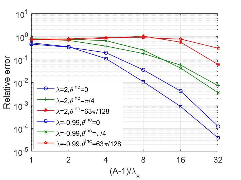
Figure 2: Relative errors $\epsilon_{\infty}$ (equation (5.1) below) in the total field resulting from the preliminary WGF method for the Dirichlet problem of scattering by a semi-circular bump. Clearly, the preliminary WGF approach is not uniformly accurate as grazing incidence is approached.

3.2 Uniformly accurate “corrected” formulation for all incidence angles

Utilizing the windowing function $\widetilde{w}_{A}$, equation (2.8) may be re-expressed in the form

$$-\frac{1}{2}\phi+K^{\prime}[\widetilde{w}_{A}\phi]=-Tu^{inc}-K^{\prime}[(1-\widetilde{w}_{A})\phi]\quad\mbox{on}\quad\Gamma.$$ (3.2)

An argument based on integration-by-parts and stationary-phase presented in [11] shows that for any positive integer $m$ there exists a constant $C_{m}$ independent of $A$, such that both the right-hand side term $K^{\prime}[(1-\widetilde{w}_{A})\phi]$ and the windowing approximation error $|\phi-\phi^{*}|$ (which results as that right-hand side term is neglected, as in (3.1)) are smaller than $C_{m}A^{-m}$ as $A\rightarrow\infty$, uniformly throughout the center region $\{\widetilde{w}_{A}=1\}$ of the surface $\Gamma_{A}$. However these errors are not uniform with respect to the incidence angle: larger and larger window sizes $A$ are required to correctly account for all fields reflected and refracted by the planar surface as the incidence angles are closer and and closer to grazing (i.e., as $\theta^{inc}$ approaches $\pm\pi/2$).

As proposed in [11, 35] for acoustic layer scattering problems, here we substitute the previously neglected right-hand side term in (3.2) by the expression that results as the density $\phi$ is corrected, that is, it is replaced by the corresponding “flat-layer” density $\phi_{\Pi}=(Tu_{f}^{tot})|_{\Pi}=(Tu_{f}^{\mathrm{scat}})|_{\Pi}+(Tu^{inc})|_{\Pi}$ that is obtained for the problems of scattering by the flat surface $\Pi$. We thus obtain the equation

$$-\frac{1}{2}\phi^{w}+K^{\prime}[\widetilde{w}_{A}\phi^{w}]=-Tu^{inc}-K^{\prime}[(1-\widetilde{w}_{A})(Tu_{f}^{tot})|_{\Pi}]\quad\mbox{on}\quad\Gamma_{A}.$$ (3.3)

for the new approximate solution $\phi^{w}$. A superalgebraically small portion of the field reflected by the windowed region reflects back into the windowed region upon reflection from the plane outside the windowed region. As a result, the substitution results in superalgebraically small errors $|\phi-\phi^{w}|$ throughout the region $\{w_{A}=1\}$.

In order to evaluate the right-hand term $K^{\prime}[(1-\widetilde{w}_{A})(Tu_{f}^{tot})|_{\Pi}]$, which is given by an integral over an unbounded domain, we note that $(1-\widetilde{w}_{A})(Tu_{f}^{tot})|_{\Pi}$ vanishes at all points at which $\Gamma_{A}$ deviates from the flat surface $\Pi$. It follows that

$$K^{\prime}[(1-\widetilde{w}_{A})(Tu_{f}^{tot})|_{\Pi}]=K^{\prime}_{\Pi}[(1-\widetilde{w}_{A})(Tu_{f}^{tot})|_{\Pi}]\quad\mbox{on}\quad\Pi,$$

where, letting now $\nu_{x}$ denote the normal to $\Pi$, the operator $K^{\prime}_{\Pi}$ is defined by

$$K^{\prime}_{\Pi}[\phi](x) = \int_{\Pi}T(\partial_{x},\nu_{x})E(x,y)\phi(y)ds_{y}.$$ (3.4)

But, clearly, $K^{\prime}_{\Pi}[\widetilde{w}_{A}(Tu_{f}^{tot})|_{\Pi}]$ can be evaluated by means of numerical integration over the bounded region $\Pi_{A}=\{x\in\Pi:\widetilde{w}_{A}(x)\neq 0\}$, and, using Green’s theorem [21], a closed form expression for $K^{\prime}_{\Pi}[(Tu_{f}^{tot})|_{\Pi}]$ results,

$$K^{\prime}_{\Pi}[(Tu_{f}^{tot})|_{\Pi}]=\begin{cases}-Tu^{inc}+\frac{1}{2}Tu_{f}^{tot}&\mbox{on}\quad\Gamma\cap\Pi,\cr Tu_{f}^{\mathrm{scat}}&\mbox{on}\quad(\Gamma\backslash\Pi)\cap{\mathbb{R}}^{d}_{+},\cr-Tu^{inc}&\mbox{on}\quad(\Gamma\backslash\Pi)\cap{\mathbb{R}}^{d}_{-},\end{cases}$$

—and, therefore, the integral in (3.4) can be easily be produced as a difference between these two quantities.

For the evaluation of the near-field, we follow [11] and substitute $\phi$ in the representation

$$u^{\mathrm{scat}}(x)=\int_{\Gamma}E(x,y)\phi(y)ds_{y}$$

by $w_{A}\phi^{w}+(1-w_{A})(Tu_{f}^{tot}|_{\Pi})$ which yields

$$u^{\mathrm{scat}}(x) = \int_{\Gamma_{A}}E(x,y)w_{A}(y)\phi^{w}(y)ds_{y}-\int_{\Pi}E(x,y)w_{A}(y)Tu_{f}^{tot}(y)ds_{y}$$ (3.5)

$$+\begin{cases}u_{f}^{\mathrm{scat}}&\mbox{in}\quad\Omega\cap{\mathbb{R}}^{d}_{+},\cr-u^{inc}&\mbox{in}\quad\Omega\cap{\mathbb{R}}^{d}_{-}.\end{cases}$$

The character of the overall approach is demonstrated in Figure 3, which presents the the relative errors in the total field $u^{tot}$ on the line segment $\{x\in{\mathbb{R}}^{2}:-1\leq x_{1}\leq 1,x_{2}=2\}$ (which were evaluated by comparison with a WGF solution with $(A-1)/\lambda_{s}=32$). Comparison with the results of the preliminary WGF method demonstrated in Figure 2 demonstrates the improvements provided by the present uniformly-accurate algorithm: much faster convergence which, as desired, is uniform for all incident angles; additional numerical illustrations of the character of the algorithm are presented in Section 5.

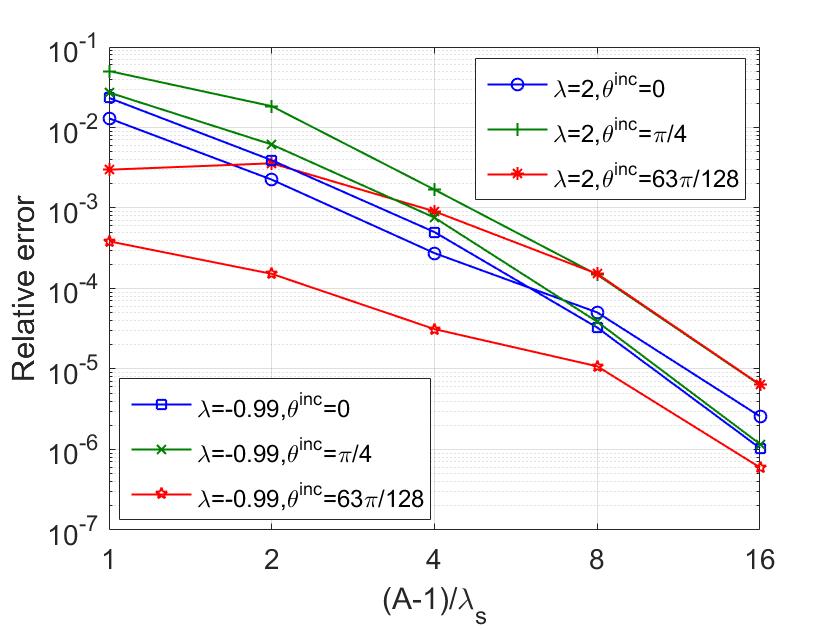
Figure 3: Relative errors $\epsilon_{\infty}$ in the total field resulting from the uniformly-accurate corrected WGF method for the Dirichlet problem of scattering by a semi-circular bump.

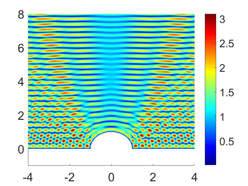
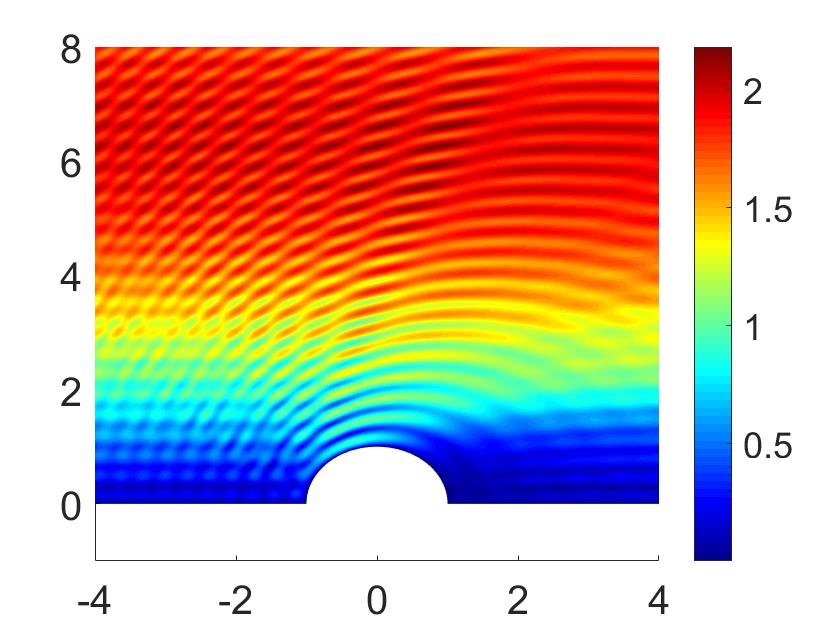
(a) $\theta^{inc}=0$	(b) $\theta^{inc}=\frac{\pi}{4}$	(c) $\theta^{inc}=\frac{63\pi}{128}$

Figure 4: Absolute values of the total field resulting from the WGF method for the Dirichlet problem of scattering of a plane pressure wave by a semi-circular bump where $\omega=20$, $\lambda=2$, $A=1+16\lambda_{s}$.

Remark 3.1.

A version of the windowed formulation of the integral equation (2.9) suitable for treatment of the Neumann problem can similarly be obtained. The resulting integral equation reads

$$\frac{1}{2}\psi^{w}+K[\widetilde{w}_{A}\psi^{w}]=u^{inc}+K_{\Pi}[(\widetilde{w}_{A}-1)(u_{f}^{tot})|_{\Pi}]\quad\mbox{on}\quad\Gamma_{A},$$ (3.6)

where the operator $K_{\Pi}$ is defined by

$$K_{\Pi}[\psi](x) = \int_{\Pi}(T(\partial_{y},\nu_{y})E(x,y))^{\top}\psi(y)ds_{y}.$$

The term $K_{\Pi}[\widetilde{w}_{A}(u_{f}^{tot})|_{\Pi}]$ can be evaluated by means of numerical integration over the bounded region $\Pi_{A}$ and the expression $K_{\Pi}[(u_{f}^{tot})|_{\Pi}]$ can be computed in closed form:

$$K_{\Pi}[(u_{f}^{tot})|_{\Pi}]=\begin{cases}u^{inc}-\frac{1}{2}u_{f}^{tot}&\mbox{on}\quad\Gamma\cap\Pi,\cr u^{inc}-u_{f}^{tot}&\mbox{on}\quad(\Gamma\backslash\Pi)\cap{\mathbb{R}}^{d}_{+},\cr u^{inc}&\mbox{on}\quad(\Gamma\backslash\Pi)\cap{\mathbb{R}}^{d}_{-}.\end{cases}$$

Furthermore, substituting $\psi=w_{A}\psi^{w}+(1-w_{A})u_{f}^{tot}|_{\Pi}$ in the scattered field representation

$$u^{\mathrm{scat}}(x)=-\int_{\Gamma}(T(\partial_{y},\nu_{y})E(x,y))^{\top}\widetilde{w}_{A}\psi(y)ds_{y}$$

for the Neumann problem yields

$$u^{\mathrm{scat}}(x) = -\int_{\Gamma}(T(\partial_{y},\nu_{y})E(x,y))^{\top}\widetilde{w}_{A}\psi^{w}(y)ds_{y}+\int_{\Pi}(T(\partial_{y},\nu_{y})E(x,y))^{\top}\widetilde{w}_{A}u_{f}^{tot}(y)ds_{y}$$ (3.7)

$$+\begin{cases}u_{f}^{\mathrm{scat}}&\mbox{in}\quad\Omega\cap{\mathbb{R}}^{d}_{+},\cr-u^{inc}&\mbox{in}\quad\Omega\cap{\mathbb{R}}^{d}_{-}.\end{cases}$$

for the evaluation of near-field.

Remark 3.2.

The expressions (3.5) and (3.7) generally do not provide accurate approximations of either far-fields or near fields outside bounded subsets of $[-cA,cA]\times{\mathbb{R}}^{d-1}$. This difficulty can be tackled [11] via an application of the Green theorem on a curve $S$ contained in $[-cA,cA]\times\{x_{d}>0\}$ and surrounding the defect, together with the layer Green function-based method discussed in Section 2.3—which, for such near- and far-field cases, for which the source and observation points are at a large or even infinite distances from each other, the layer Green function can be obtained rapidly.

4 Numerical implementation

The iterative solvers for solution of the discrete versions of (3.3) and (3.6) rely on the numerical evaluation of integral operators and the iterative linear algebra solver GMRES. This section presents the 2D algorithms for the numerical evaluation, for a given density $\psi$, of the quantities $K[\widetilde{w}_{A}\psi]$, $K^{\prime}[\widetilde{w}_{A}\psi]$, $K_{\Pi}[\widetilde{w}_{A}\psi]$ and $K_{\Pi}^{\prime}[\widetilde{w}_{A}\psi]$ associated with the WGF method for the solution of the Dirichlet and Neumann problems. For the numerical implementation in 3D, in turn, we utilize the methods presented in [12, 17].

4.1 Reformulation in terms of composite differential/weakly-singular operators

As discussed in Section 1, the methods [39] can be used to express the quantities

$$K[\widetilde{w}_{A}\psi](x) = \int_{\Gamma_{A}}(T(\partial_{y},\nu_{y})E(x,y))^{\top}\widetilde{w}_{A}(y)\psi(y)ds_{y},\quad x\in\Gamma_{A},$$ (4.1)

$$K^{\prime}[\widetilde{w}_{A}\psi](x) = \int_{\Gamma_{A}}T(\partial_{x},\nu_{x})E(x,y)\widetilde{w}_{A}(y)\psi(y)ds_{y},\quad x\in\Gamma_{A},$$ (4.2)

in the forms

$$K[\widetilde{w}_{A}\psi](x) = K_{1}[\widetilde{w}_{A}\psi](x)+K_{2}\left[T_{0}(\widetilde{w}_{A}\psi)\right](x),$$ (4.3)

$$K^{\prime}[\widetilde{w}_{A}\psi](x) = K_{1}^{\prime}[\widetilde{w}_{A}\psi](x)+T_{0}K^{\prime}_{2}\left[\widetilde{w}_{A}\psi\right](x),$$ (4.4)

where the operators $K_{1},K_{2},K^{\prime}_{1},K^{\prime}_{2}$ are given by

$$K_{1}[\phi](x) = \int_{\Gamma_{A}}H_{1}(x,y)\phi(y)ds_{y},\quad H_{1}(x,y)=\frac{\partial\gamma_{k_{s}}(x,y)}{\partial\nu_{y}}I-\nabla_{y}[\gamma_{k_{s}}(x,y)-\gamma_{k_{p}}(x,y)]\nu_{y}^{\top},$$

$$K_{2}[\phi](x) = \int_{\Gamma_{A}}H_{2}(x,y)\phi(y)ds_{y},\quad H_{2}(x,y)=[2\mu E(x,y)-\gamma_{k_{s}}(x,y)I]\begin{pmatrix}0&-1\\ 1&0\end{pmatrix},$$

$$K_{1}^{\prime}[\phi](x) = \int_{\Gamma_{A}}H_{3}(x,y)\phi(y)ds_{y},\quad H_{3}(x,y)=\frac{\partial\gamma_{k_{s}}(x,y)}{\partial\nu_{x}}I-\nu_{x}\nabla_{y}^{\top}[\gamma_{k_{s}}(x,y)-\gamma_{k_{p}}(x,y)],$$

$$K_{2}^{\prime}[\phi](x) = \int_{\Gamma_{A}}H_{4}(x,y)\phi(y)ds_{y},\quad H_{4}(x,y)=\begin{pmatrix}0&-1\\ 1&0\end{pmatrix}[2\mu E(x,y)-\gamma_{k_{s}}(x,y)I],$$

and where

$$T_{0}=\nu^{\perp}\cdot\nabla$$

denotes the tangential derivative. The quantities $K_{\Pi}[\widetilde{w}_{A}\psi]$ and $K_{\Pi}^{\prime}[\widetilde{w}_{A}\psi]$ can be re-expressed in a similar manner. In view of these reformulations, the integral operators introduced in Section 3.2 can be evaluated numerically as a sum of compositions involving the numerical differentiation operator $T_{0}$ as well as integral operators of the form

$$\mathcal{H}[\psi](x)=\int_{\Gamma_{0}}H(x,y)\psi(y)ds_{y},\quad\Gamma_{0}=\Gamma_{A}\quad\mbox{or}\quad\Pi_{A},$$ (4.5)

in which the kernel $H(x,y)$ is only weakly singular. The remainder of this section presents the algorithms we propose for numerical evaluation of operators of these two types, including a two dimensional version of the rectangular-polar Chebyshev-based quadrature method [12] for weakly singular operators of the form (4.5) and Chebyshev-based differentiation algorithms.

4.2 Surface decomposition and discretization

The proposed algorithm evaluates weakly singular integrals of the form (4.5) by first partitioning $\Gamma_{0}$ into a finite number $M$ of parametrized patches $\Gamma_{q}$, $q=1,\dots,M$:

$$\Gamma_{0}=\bigcup_{q=1}^{M}\Gamma_{q},\quad\Gamma_{q}=\{x^{q}(t):[-1,1]\rightarrow{\mathbb{R}}^{2}\}.$$

(It is assumed that each corner point $x\in\Gamma_{0}$, if any such point exists, is located at parametrization endpoints $t=1$ or $-1$ of the patches $\Gamma_{q}$ that contain $x$.) Clearly, then, the integral (4.5) can be expressed as a sum of integrals over each of the patches:

$$\mathcal{H}(x)=\sum_{q=1}^{M}\mathcal{H}_{q}(x),\quad\mathcal{H}_{q}(x)=\int_{\Gamma_{q}}H(x,y)\phi(y)ds_{y}.$$

Using the parametrization $x=x^{q}(t)$ for the patch $\Gamma_{q}$ we obtain

$$\mathcal{H}_{q}(x)=\int_{-1}^{1}\widetilde{H}(x,t)\widetilde{\phi}(t)J^{q}(t)dt,$$ (4.6)

where $\widetilde{H}(x,t)=H(x,x^{q}(t))$, $\widetilde{\phi}(t)=\phi(x^{q}(t)$ and $J^{q}(t)=|dx^{q}(t)/dt|)\neq 0$ denotes the surface Jacobian.

To treat the singular character of integral-equation densities at corners in a general and robust manner, we introduce a change of variables [12] on the parametrization variables $t$, a number of whose derivatives vanish at the corners. In detail, defining the function

$$w_{p}(\tau)=2\pi\frac{[v_{p}(\tau)]^{p}}{[v_{p}(\tau)]^{p}+[v_{p}(2\pi-\tau)]^{p}},\quad 0\leq\tau\leq 2\pi,$$

where

$$v_{p}(\tau)=\left(\frac{1}{p}-\frac{1}{2}\right)\left(\frac{\pi-\tau}{\pi}\right)^{3}+\frac{1}{p}\left(\frac{\tau-\pi}{\pi}\right)+\frac{1}{2},$$

(whose derivatives vanish up to order $p-1$ at the endpoints $\tau=0$ and $\tau=2\pi$), we define the smoothing change-of-variables $t=\eta_{t}^{q}(\tau)$ for the patch $\Gamma_{q}$ according to the expressions

$$t=\eta_{t}^{q}(\tau)=\begin{cases}\tau,&\mbox{No corner at either $\Gamma_{q}$ endpoint},\cr-1+\frac{1}{\pi}w_{p}(\pi(\tau+1)),&\mbox{Corners at both $\Gamma_{q}$ endpoints},\cr-1+\frac{2}{\pi}w_{p}(\pi(\tau+1)/2),&\mbox{Corner at the $t=-1$ $\Gamma_{q}$ endpoint only},\cr-3+\frac{2}{\pi}w_{p}(\pi+\pi(\tau+1)/2),&\mbox{Corner at the $t=1$ $\Gamma_{q}$ endpoint only}.\end{cases}$$ (4.7)

Incorporating the change of variables (4.7), we obtain

$$\mathcal{H}_{q}(x)=\int_{-1}^{1}\widetilde{H}(x,\eta_{t}^{q}(\tau))\widetilde{\phi}(\eta_{t}^{q}(\tau))J^{q}(\eta_{t}^{q}(\tau))\frac{d\eta_{t}^{q}(\tau)}{d\tau}d\tau,$$ (4.8)

Considering the distance

$$\mbox{dist}_{x,\Gamma_{q}}:=\min_{u\in[-1,1]}\left\{|x-x^{q}(u)|\right\},$$

between the point $x$ and the patch $\Gamma_{q}$, a number of “singular”, “near-singular” and “regular” integration problems arise as described in Section 4.3. For accuracy and efficiency our algorithm evaluates these integrals are produced by means of Fejér’s first quadrature rule, which effectively exploits the discrete orthogonality property satisfied by the Chebyshev polynomials in the Chebyshev meshes. Denoting by $u_{j}\in[-1,1]$ ($j=0,\cdots,N-1$) the $N$ Chebyshev points

$$u_{j}=\cos\left(\frac{2j+1}{2N}\pi\right),\quad j=0,\cdots,N-1,$$

we utilize discretization points in each patch $\Gamma_{q}$ according to $x_{i}^{q}=x^{q}(\eta_{t}^{q}(u_{i})),\quad i=0,\cdots,N-1$. Then, a given density $\varphi$ with values $\varphi_{i}^{q}=\varphi(x_{i}^{q})$ is approximated by means of the Chebyshev expansion

$$\varphi(x)\approx\sum_{i=0}^{N-1}\varphi_{i}^{q}a_{i}(u),\quad x\in\Gamma_{q},$$

where the quantities

$$a_{i}(u)=\frac{1}{N}\sum_{n=0}^{N-1}\alpha_{n}T_{n}(u_{i})T_{n}(u),\quad\alpha_{n}=\begin{cases}1,&n=0,\cr 2,&n\neq 0.\end{cases}$$

satisfy the discrete-orthogonality relations

$$a_{i}(u_{n})=\begin{cases}1,&n=i,\cr 0,&\mathrm{otherwise}.\end{cases}$$

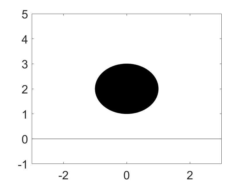
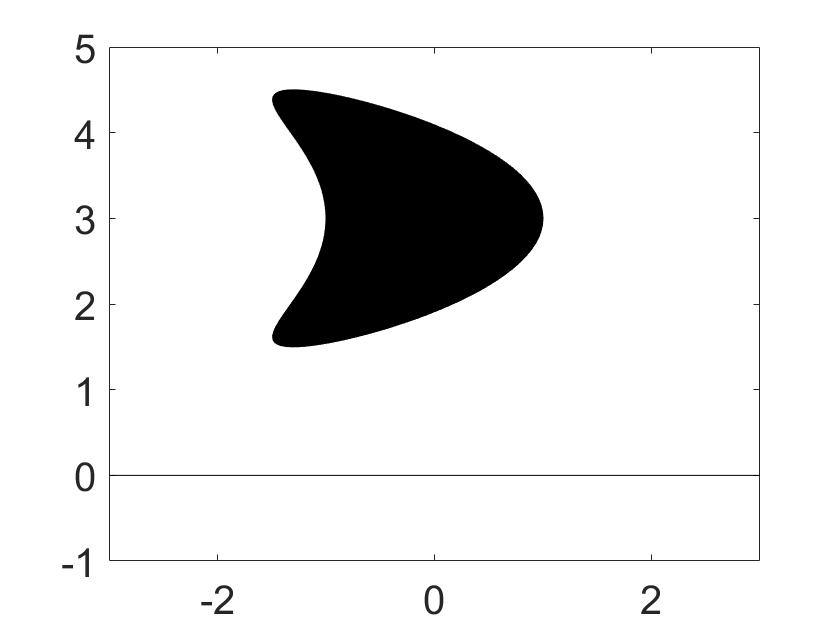
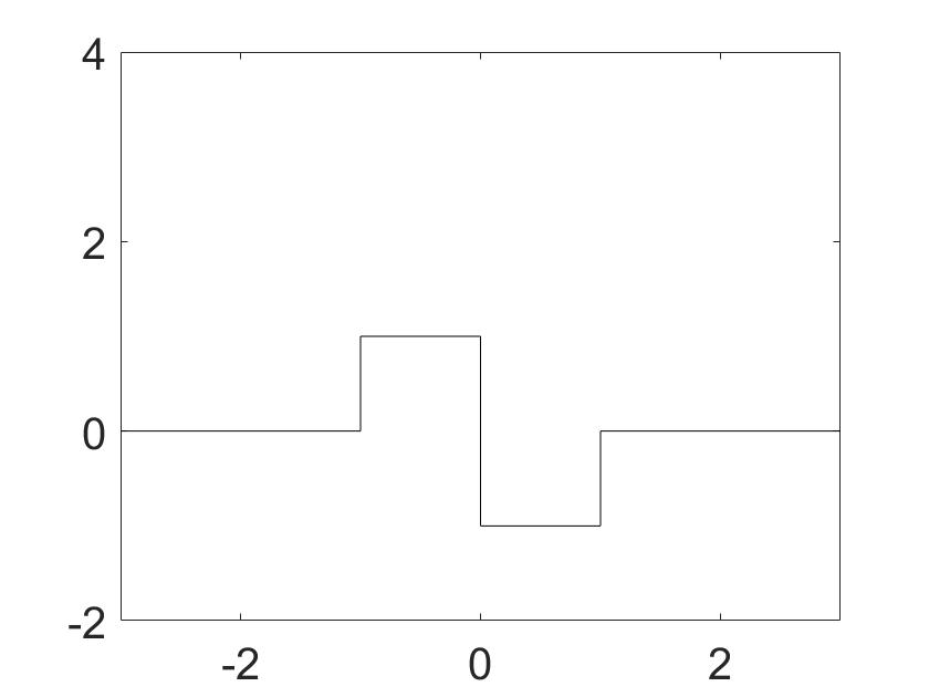
(a) disc within half-space	(b) kite within half-space	(c) local boundary perturbation

Figure 5: Various 2D half-space considered in this paper.

4.3 Non-adjacent and adjacent integration

Let $x$ be one of the discretization points on $\Gamma_{A}$. In the "non-adjacent" integration case, in which the point $x$ is far from the integration patch (i.e., $\mbox{dist}_{x,\Gamma_{q}}>\tau$ for some tolerance $\tau>0$), the integrand $\mathcal{H}_{q}(x)$ is smooth, and the integral over $\Gamma_{q}$ can be accurately evaluated by means of Fejér’s first quadrature rule

$$\mathcal{H}_{q}(x) \approx \sum_{n=0}^{N-1}w_{n}\widetilde{H}(x,\eta_{t}^{q}(u_{n}))\varphi_{n}^{q}J^{q}(\eta_{t}^{q}(u_{n}))\left(\frac{d\eta_{t}^{q}(\tau)}{d\tau}\Big{|}_{\tau=u_{n}}\right),$$ (4.9)

where $w_{j},j=0,\cdots,N-1$ are the quadrature weights

$$w_{j}=\frac{2}{N}\left(1-2\sum_{l=1}^{\lfloor N/2\rfloor}\frac{1}{4l^{2}-1}\cos(lu_{j})\right),\quad j=0,\cdots,N-1.$$

In the "adjacent" integration case, in which the point $x$ either lies within the integration patch or is "close" to it (i.e., $\mbox{dist}_{x,\Gamma_{q}}\leq\tau$), the problem of evaluation of $\mathcal{H}_{q}(x)$ presents a challenge in view of the singularity or nearly-singularity of its kernel. To tackle this difficulty we apply a change of variables whose derivatives vanish at the singularity or, for nearly singular problems, at the point in the integration patch that is closest to the singularity—in either case, the coordinates $u^{q}\in[-1,1]$ of the point around which refinements are performed are given by

$$\widetilde{u}^{q}={\arg\min}_{u\in[-1,1]}\left\{|x-x^{q}(\eta_{t}^{q}(u))|\right\}.$$

The quantities $\widetilde{u}^{q}$ can be found by means of an appropriate minimization algorithm such as the golden section search algorithm. Making use of the mapping $w_{p}$ defined in Section 4.2 we construct the change of variables

$$\xi_{\alpha}(t)=\begin{cases}\alpha+\frac{\mbox{sgn}(t)-\alpha}{\pi}w_{p}(\pi|t|),&\alpha\neq\pm 1,\cr\alpha-\frac{1+\alpha}{\pi}w_{p}\left(\pi\frac{|t-1|}{2}\right),&\alpha=1,\cr\alpha+\frac{1-\alpha}{\pi}w_{p}\left(\pi\frac{|t+1|}{2}\right),&\alpha=-1,\end{cases}$$

where $\mbox{sgn}(x)$ equals $1$, $-1$ or $0$ according to whether $x>0$, $x<0$ or $x=0$, respectively. Applying the Chebyshev expansion of the density $\varphi$, the above change of variables and the Fejér’s first quadrature rule, we obtain

$$\mathcal{H}_{q}(x) \approx \sum_{n=0}^{N-1}\varphi_{n}^{q}\sum_{m=0}^{N^{\beta}-1}\widetilde{w}_{m}\widetilde{H}(x,s^{q}_{m})\widetilde{J}^{q}(s^{q}_{m})\widetilde{a}_{n}(s^{q}_{m})\xi_{\widetilde{u}^{q}}^{\prime}(\widetilde{u}_{m})\left(\frac{d\eta_{t}^{q}(\tau)}{d\tau}\Big{|}_{\tau=\xi_{\widetilde{u}^{q}}(\widetilde{u}_{m})}\right)$$ (4.10)

where

$$s^{q}_{m}=\eta_{t}^{q}(\xi_{\widetilde{u}^{q}}(\widetilde{u}_{m})),$$

and where the quadrature nodes and weights are given by

$$\widetilde{u}_{j}=\cos\left(\frac{2j+1}{2N^{\beta}}\pi\right),\quad j=0,\cdots,N^{\beta}-1,$$

and

$$\widetilde{w}_{j}=\frac{2}{N^{\beta}}\left(1-2\sum_{l=1}^{\lfloor N^{\beta}/2\rfloor}\frac{1}{4l^{2}-1}\cos(l\widetilde{u}_{j})\right),\quad j=0,\cdots,N^{\beta}-1,$$

respectively. Using sufficiently large numbers $N^{\beta}$ of discretization points to accurately resolve the challenging integrands, all singular and nearly singular problems can be treated with high accuracy under discretizations that are not excessively fine.

$\omega$	$A/\lambda_{s}$	Disc-shaped			Kite-shaped
		$\theta^{inc}=0$	$\theta^{inc}=\frac{\pi}{4}$	$\theta^{inc}=\frac{63\pi}{128}$	$\theta^{inc}=0$	$\theta^{inc}=\frac{\pi}{4}$	$\theta^{inc}=\frac{63\pi}{128}$
	2	1.54E-2	2.61E-2	1.18E-2	3.79E-2	5.13E-2	8.76E-3
	4	1.62E-3	8.10E-3	3.92E-3	3.29E-3	1.46E-2	8.92E-3
4	8	1.49E-4	5.20E-4	2.73E-4	1.48E-4	3.60E-4	5.58E-4
	16	2.12E-6	2.49E-6	1.14E-6	1.85E-6	1.30E-6	4.43E-6
	32	2.99E-8	4.29E-8	1.98E-8	3.27E-8	2.06E-8	1.11E-7
	2	1.98E0	1.35E0	2.71E-1	8.34E-1	1.65E0	1.06E0
	4	4.92E-2	2.81E-2	2.25E-2	5.30E-1	1.54E0	1.33E0
20	8	4.72E-3	1.09E-2	2.85E-3	7.80E-3	1.24E-2	1.63E-3
	16	3.22E-5	1.45E-4	6.90E-5	7.17E-5	2.13E-4	2.93E-4
	32	9.55E-7	1.46E-6	1.81E-6	9.30E-7	2.12E-6	1.53E-6

Table 1: Relative errors $\epsilon_{\infty}$ in the total field resulting from the WGF method for the Dirichlet problems of scattering by a disc-shaped and a kite-shaped obstacle within a half space.

$\omega$	$A/\lambda_{s}$	Disc-shaped			Kite-shaped
		$\theta^{inc}=0$	$\theta^{inc}=\frac{\pi}{4}$	$\theta^{inc}=\frac{63\pi}{128}$	$\theta^{inc}=0$	$\theta^{inc}=\frac{\pi}{4}$	$\theta^{inc}=\frac{63\pi}{128}$
	2	4.31E-2	2.95E-2	1.78E-2	5.85E-2	5.47E-2	4.05E-2
	4	4.48E-3	7.24E-3	5.87E-3	7.75E-3	1.60E-2	8.51E-3
4	8	3.87E-4	3.36E-4	2.60E-4	2.67E-4	6.06E-4	6.67E-4
	16	8.16E-6	3.65E-6	2.83E-6	6.48E-6	7.84E-6	8.37E-6
	32	1.31E-7	5.07E-8	1.51E-7	5.97E-8	1.04E-7	1.30E-7
	2	2.02E0	2.24E0	2.95E-1	7.31E-1	1.50E0	1.39E0
	4	1.66E-1	2.88E-1	1.91E-1	4.27E-1	1.55E0	1.41E0
20	8	5.37E-3	2.15E-2	3.37E-3	6.40E-3	1.16E-2	4.98E-3
	16	7.64E-5	1.67E-4	8.09E-5	9.05E-5	1.96E-4	5.73E-4
	32	2.21E-6	3.18E-6	2.37E-6	1.01E-6	3.52E-6	2.38E-6

Table 2: Relative errors $\epsilon_{\infty}$ in the total field resulting from the WGF method for the Neumann problems of scattering by a disc-shaped and a kite-shaped obstacle within a half space.

4.4 Evaluation of tangential derivatives

Finally, we describe the implementation we use for the evaluation of the tangential derivative operator $T_{0}$. On each patch $\Gamma_{q}$, applying the surface parametrization for a given density $\varphi$ we have

$$\varphi(x)=\phi(x^{q}(\eta_{t}^{q}(\tau)))=\phi(x^{q}(\eta_{t}^{q}(\cos\theta))),\quad\theta\in[0,\pi].$$

It follows the tangential derivative of $\varphi$ on $\Gamma_{q}$ is given by

$$(T_{0}\varphi)(x)=-\frac{1}{J^{q}(\eta_{t}^{q}(\cos\theta))\sin\theta\left(\frac{d\eta_{t}^{q}(\tau)}{d\tau}\Big{|}_{\tau=\cos\theta}\right)}\frac{d\varphi(x^{q}(\eta_{t}^{q}(\cos\theta)))}{d\theta}.$$

(Note that the tangential derivative operator is evaluated at the Chebyshev points $\theta_{j}=\pi\frac{2j+1}{2N}$, $j=0,1,\cdots,N-1$, at which $J^{q}(\eta_{t}^{q}(\cos\theta_{j}))\sin\theta_{j}\left(\frac{d\eta_{t}^{q}(\tau)}{d\tau}\Big{|}_{\tau=\cos\theta_{j}}\right)\neq 0$.) Given the values of density $\phi(x^{q}(\eta_{t}^{q}(\cos\theta)))$ at the Chebyshev points $\theta_{j}=\pi\frac{2j+1}{2N}$, $j=0,1,\cdots,N-1$, the necessary derivative with respect to $\theta$ can be evaluated by extending the density as an even function in $[-\pi,\pi]$ and using FFT.

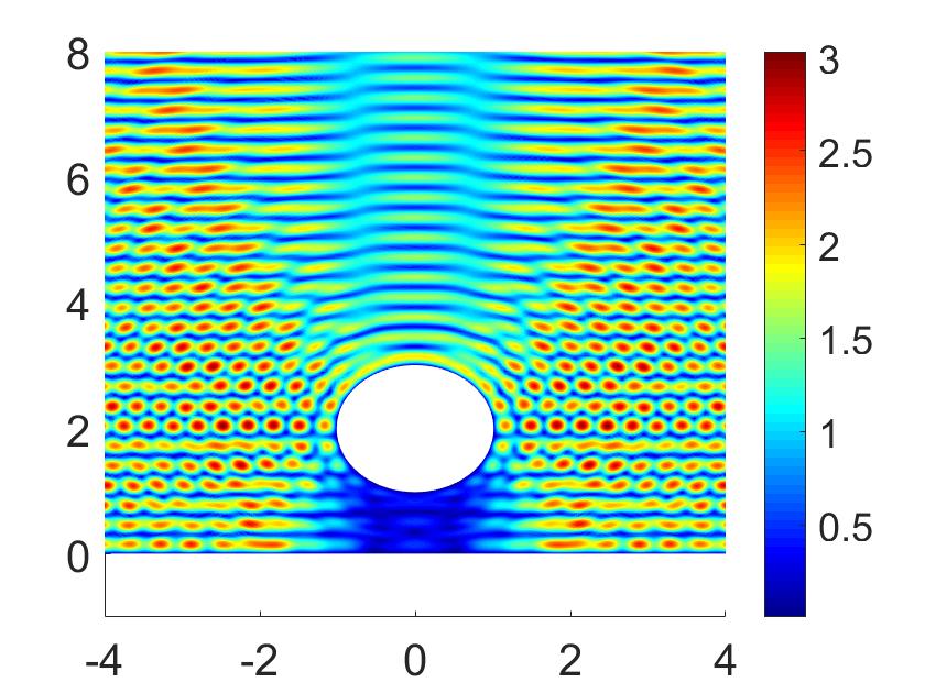
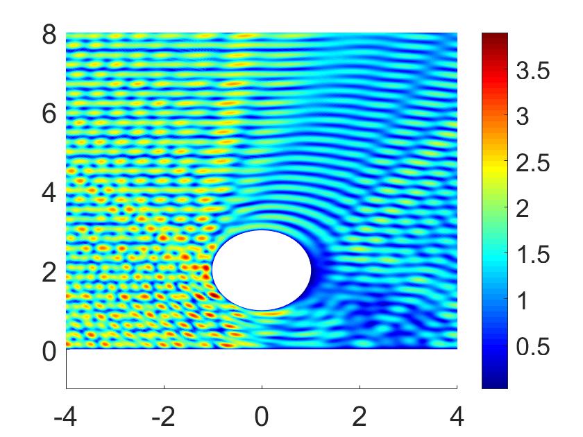
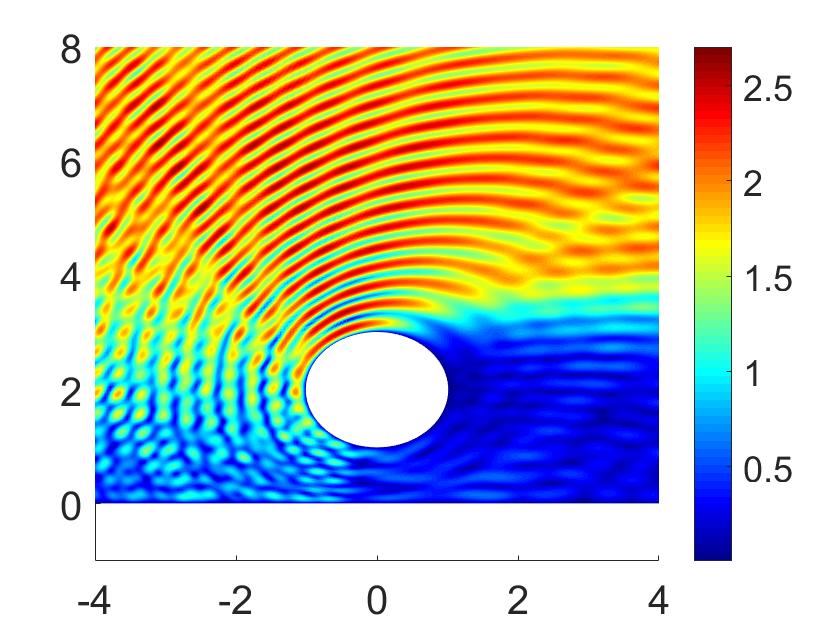
(a) $\theta^{inc}=0$	(b) $\theta^{inc}=\frac{\pi}{4}$	(c) $\theta^{inc}=\frac{63\pi}{128}$

Figure 6: Absolute values of the total field resulting from the WGF method for the Dirichlet problem of scattering by a disc-shaped obstacle where $\omega=20$, $A=32\lambda_{s}$.

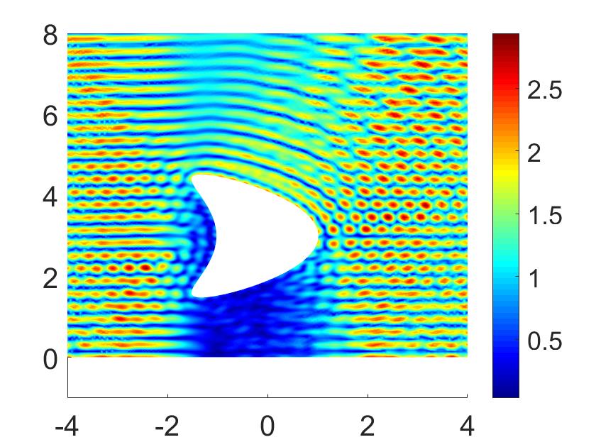
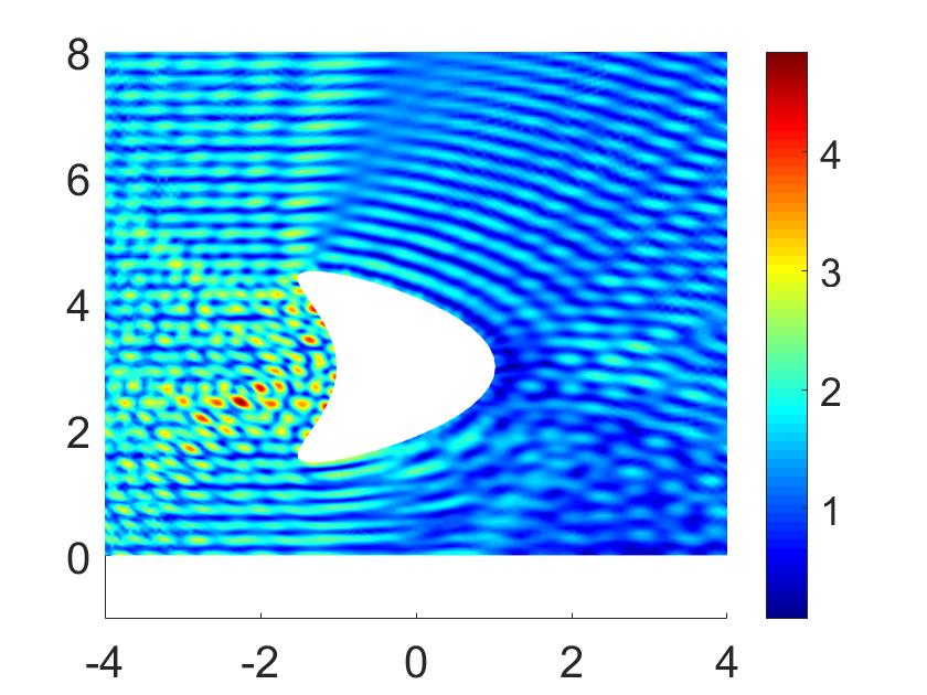
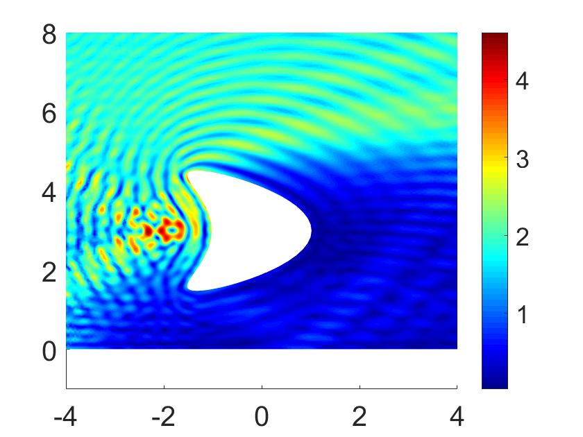
(a) $\theta^{inc}=0$	(b) $\theta^{inc}=\frac{\pi}{4}$	(c) $\theta^{inc}=\frac{63\pi}{128}$

Figure 7: Absolute values of the total field resulting from the WGF method for the Neumann problem of scattering by a kite-shaped obstacle where $\omega=20$, $A=32\lambda_{s}$.

5 Numerical results

The two-dimensional numerical results presented in section 3, and, particularly, Figures 3 and 4, demonstrate the advantages inherent in the uniformly-accurate fixed-windowed integral formulation (3.3), namely, fast convergence uniformly over all incidence angles. The present section, in turn, presents a variety of additional numerical examples in both 2D and 3D, which demonstrate the efficiency and accuracy of the proposed WGF method. Solutions for the integral equations were produced by means of the fully complex version of the iterative solver GMRES. All of the numerical tests were obtained by means of Fortran numerical implementations, parallelized using OpenMP, on a single node (twenty-four computing cores) of a dual socket Dell R420 with two Intel Xenon E5-2670 v3 2.3 GHz, 128GB of RAM. In all cases, unless otherwise stated, the values $\lambda=2$, $\mu=1$, $\rho=1$, $p=8$, $c=0.7$ were used and the relative errors reported were calculated in accordance with the expression

$$\epsilon_{\infty}=\frac{\max_{x\in S}|u^{\mbox{num}}(x)-u^{\mbox{ref}}(x)|}{\max_{x\in S}|u^{\mbox{ref}}(x)|},$$ (5.1)

where $u^{\mbox{ref}}$ is produced by means of numerical solution with a sufficiently fine discretization and a sufficiently large value of $A$, and where $S$ is a suitably selected line segment (2D) or square plane (3D) above the defect, and at a distance from it no larger than 2. The parameters $M$, $N$, $N^{\beta}$ were selected in such a way that the errors arising from the numerical integration are negligible in comparison with the smooth-windowing errors. Throughout this section aEn denotes $a\times 10^{n}$.

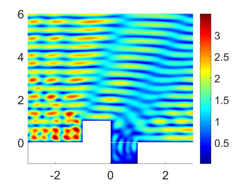
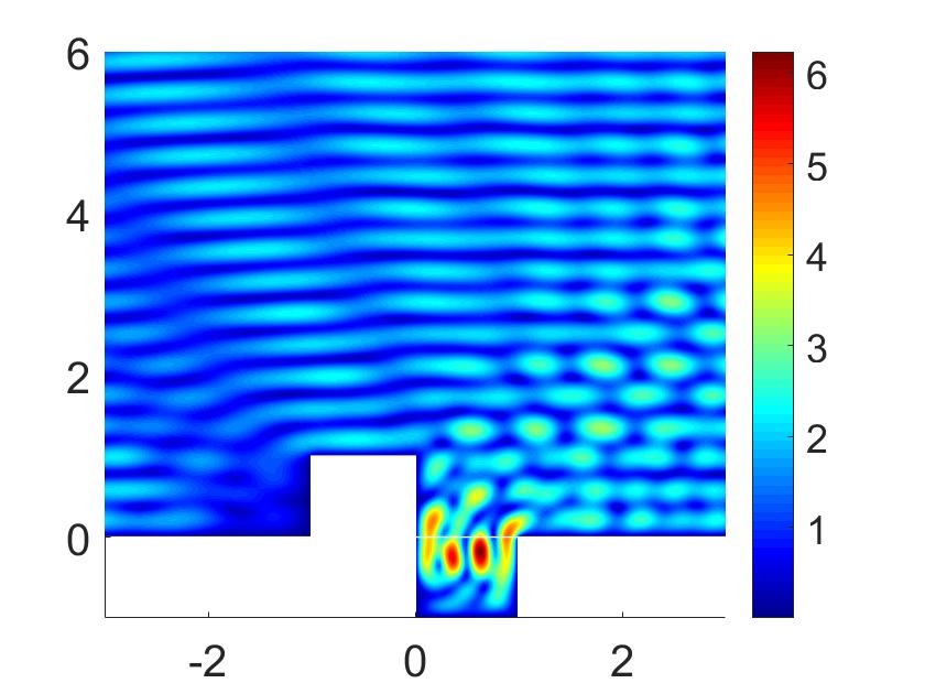
(a) $\theta^{inc}=\frac{\pi}{4}$	(b) $\theta^{inc}=-\frac{\pi}{4}$

Figure 8: Absolute values of the total field resulting from the WGF method for the Dirichlet problem of scattering by a locally perturbed surface where $\omega=4\pi$, $A=1+16\lambda_{s}$; $\epsilon_{\infty}=$ 1E-5.

5.1 2D examples

In our first example we consider problems of elastic scattering by the two-dimensional locally-rough surfaces depicted in Figure 5. These include problems of scattering of bounded scatterers under both Dirichlet and Neumann boundary conditions over a half-plane (disc-shaped and kite-shaped see Figure 5(a,b)), as well as the local corrugation depicted in Figure 5(c). In all three cases the impenetrable (Dirichlet or Neumann) infinite boundary is shown as a thin black line. Tables 1 and 2 display the relative errors in the total field that result from use of the proposed WGF method for the Dirichlet and Neumann problems, respectively, clearly demonstrating the uniform fast convergence of the proposed approach over wide angular variations, going from normal incidence to grazing. Figures 6 and 7 The near fields for the problem of scattering by the Dirichlet disc-shaped obstacle and the Neumann kite-shaped obstacle are presented in Figures 6 and 7, respectively.

We consider next the problem of scattering by a locally-rough surface containing multiple corners, see Figure 5(c). In this example we assumed $\omega=4\pi$, and we utilized a total of twelve integration patches over the local perturbation, with refinement exponent $p=4$ at corners, and with window radius $A=1+16\lambda_{s}=9$. Figure 8 displays the total fields for the Dirichlet problem with incident angles $\theta^{inc}=\pi/4$ and $\theta^{inc}=-\pi/4$, respectively. In both cases the relative error is smaller than 1E-5.

5.2 3D examples

$A/\lambda_{s}$	Dirichlet problem			Neumann problem
	$\theta^{inc}=0$	$\theta^{inc}=\frac{\pi}{4}$	$\theta^{inc}=\frac{63\pi}{128}$	$\theta^{inc}=0$	$\theta^{inc}=\frac{\pi}{4}$	$\theta^{inc}=\frac{63\pi}{128}$
2	1.61E-1	7.76E-2	8.10E-2	5.40E-2	4.44E-1	5.03E-2
3	3.03E-2	2.37E-2	3.44E-2	1.49E-2	8.24E-2	2.03E-2
4	5.15E-3	4.03E-3	7.60E-3	3.66E-3	5.28E-3	1.36E-2
5	1.24E-3	9.93E-4	1.98E-3	1.75E-3	1.90E-3	4.07E-3
6	2.27E-4	1.75E-4	3.51E-4	6.19E-4	6.38E-4	1.94E-3

Table 3: Relative errors $\epsilon_{\infty}$ in the total field resulting from the WGF method for Dirichlet and Neumann problems of scattering by a spherical obstacle within a half space.

$\theta^{inc}$	$A/\lambda_{s}$	$M$	$N_{\mathrm{DOF}}$	Time (prec.)	Time (1 iter.)	$N_{iter}$
	2	22	$3\times 12672$	32.92 s	5.12 s	29
0	4	70	$3\times 40320$	2.79 min	1.12 min	32
	6	150	$3\times 86400$	8.60 min	5.05 min	34
	2	22	$3\times 12672$	33.23 s	5.07 s	40
$\frac{\pi}{4}$	4	70	$3\times 40320$	2.84 min	1.12 min	42
	6	150	$3\times 86400$	8.55 min	5.00 min	45
	2	22	$3\times 12672$	33.02 s	5.11 s	33
$\frac{63\pi}{128}$	4	70	$3\times 40320$	2.87 min	1.13 min	33
	6	150	$3\times 86400$	8.57 min	5.04 min	34

Table 4: Computing costs required by the WGF method for the Neumann problem of scattering by a spherical obstacle, with GMRES tolerance equal to 1E-4, and with $N=24$ and $N^{\beta}=100$.

We consider two 3D inclusion types, namely, a sphere and a kite-shaped obstacle, in both cases over a half space. The total-field relative errors presented in Table 3 demonstrate the high accuracy and fast convergence of the proposed 3D WGF method, which is observed, once again, uniformly for all incidence angles. Table 4 displays the corresponding computing costs required by the solver; for definiteness we only present results for the Neumann case, but the statistics for the corresponding Dirichlet case are entirely analogous.

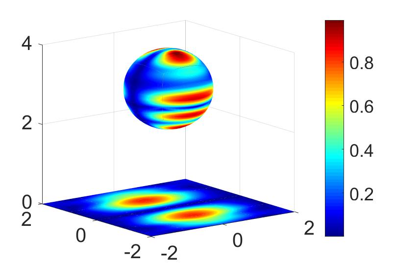
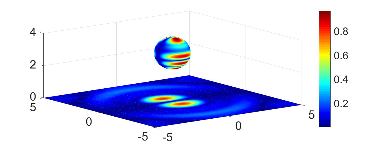
(a) $A=2$, $|u_{2}|$	(b) $A=5$, $|u_{2}|$
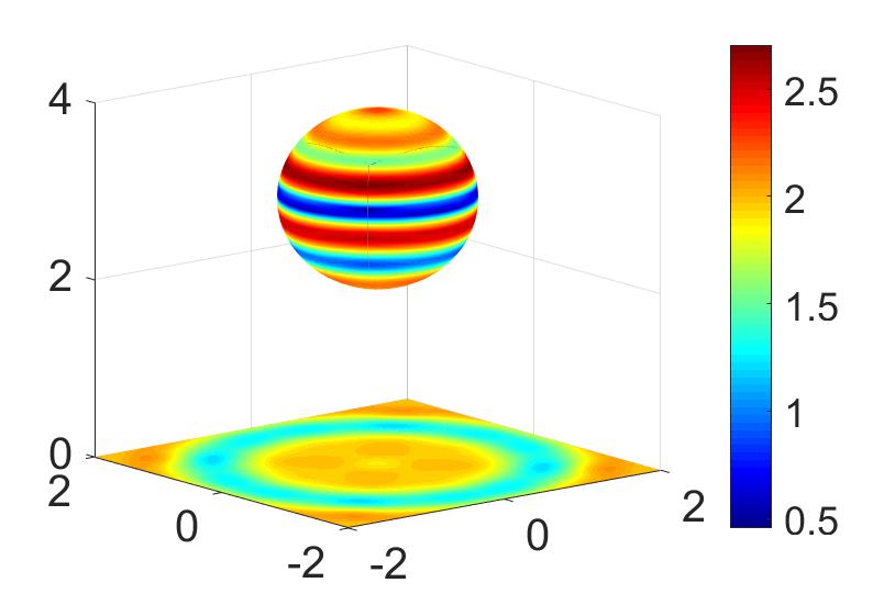
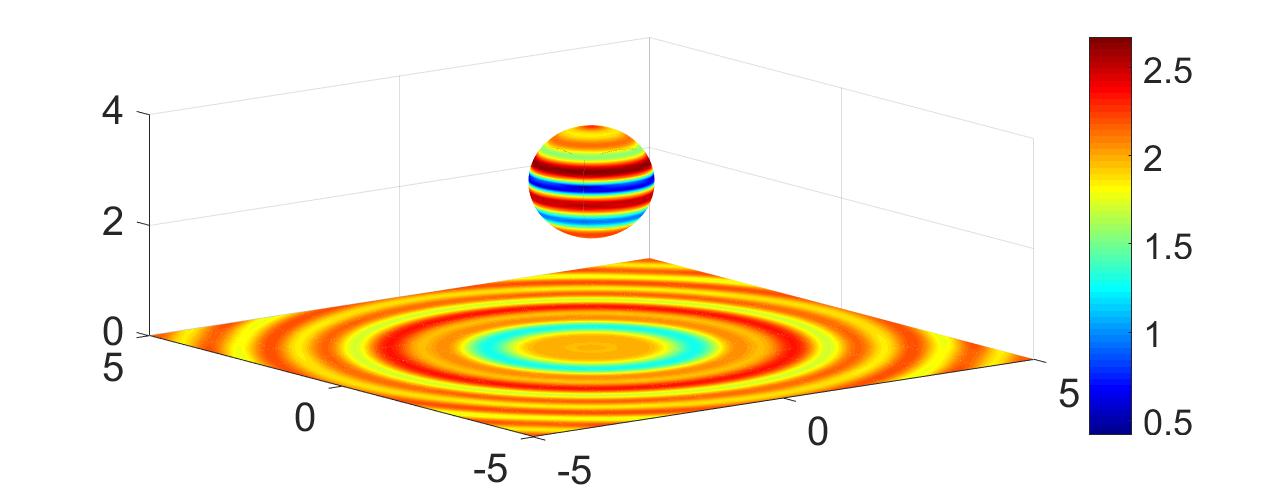
(c) $A=2$, $|u_{3}|$	(d) $A=5$, $|u_{3}|$

Figure 9: Absolute values of the second (a,b) and third (c,d) components of the total field resulting from the WGF method for the Neumann problem of scattering by a spherical obstacle. The section of the planar interface shown in each case coincides with the windowed region in the plane where the corresponding windowing function $\widetilde{w}_{A}$ does not vanish. $\theta^{inc}=0$.

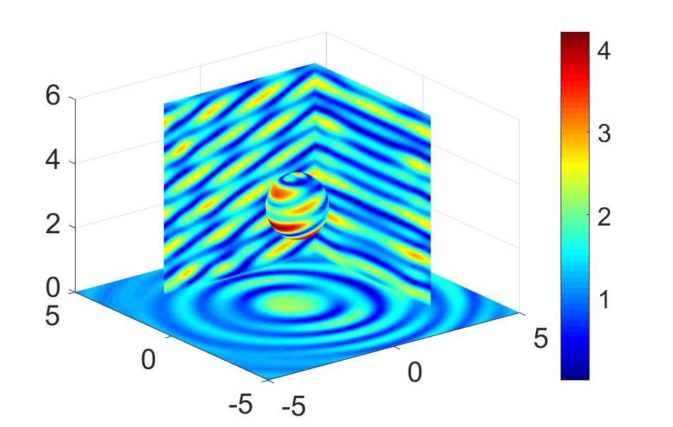
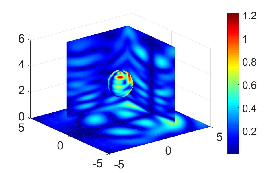
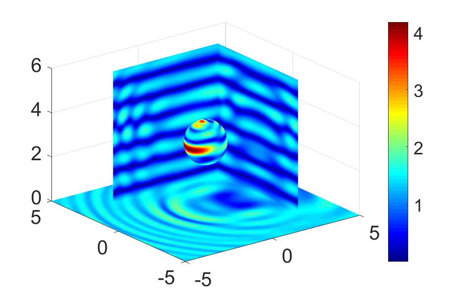
(a) $|u_{1}|$	(b) $|u_{2}|$	(c) $|u_{3}|$

Figure 10: Absolute values of the three components of the total field resulting from the WGF method for the Neumann problem of scattering by a spherical obstacle. The section of the planar interface shown in each case coincides with the windowed region in the plane where the corresponding windowing function $\widetilde{w}_{A}$ does not vanish. $\theta^{inc}=\pi/4$.

Figure 9 displays the computed values of the total field for the Neumann problem with $\lambda=\mu=3$ and $\omega=5\sqrt{3}\pi/2$. These results are consistent with the LGF-based results presented in [19], which include a treatment of this problem but only under $\theta^{inc}=0$ incidence. The LGF evaluation that is required in the treatment [20], on the other hand, is much more expensive, on a per-point basis than the free-space Green function we use. A direct truncation of the infinite planar surface to the square $|x|\leq A$ was proposed in [18, 19] for an equation similar to (3.1); as discussed in Sections 1 and Section 2 and suggested by the WGF results in Figure 2, however, such approaches lead to significant difficulties as the incidence angles sufficiently depart from normal incidence.

Finally, the total field produced by the WGF method for the Dirichlet problem of scattering by the bean-shaped obstacle over a half space displayed in Figure 11(a), for a problem with $\omega=2\pi$, $\theta^{inc}=-\pi/3$ and $A=5\lambda_{s}$, which was treated using the algorithmic parameter selections $M=106$, $N=24$ and $N^{\beta}=100$, is presented in Figures 11(b,c,d). The relative solution error $\epsilon_{\infty}$ is smaller than 1E-3 and the absolute computing time (including precomputation as well as GMRES iteration and field evaluation) is 1.94h with GMRES tolerance equal to 1E-4. Of course, all of the computing times can be greatly reduced by means of suitable acceleration method such as those presented in [20, 14] and references therein.

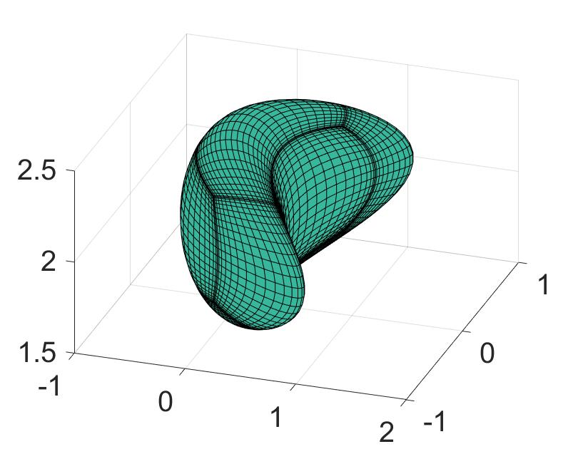
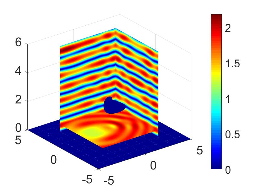
(a) Bean-shaped obstacle	(b) $|u_{1}|$
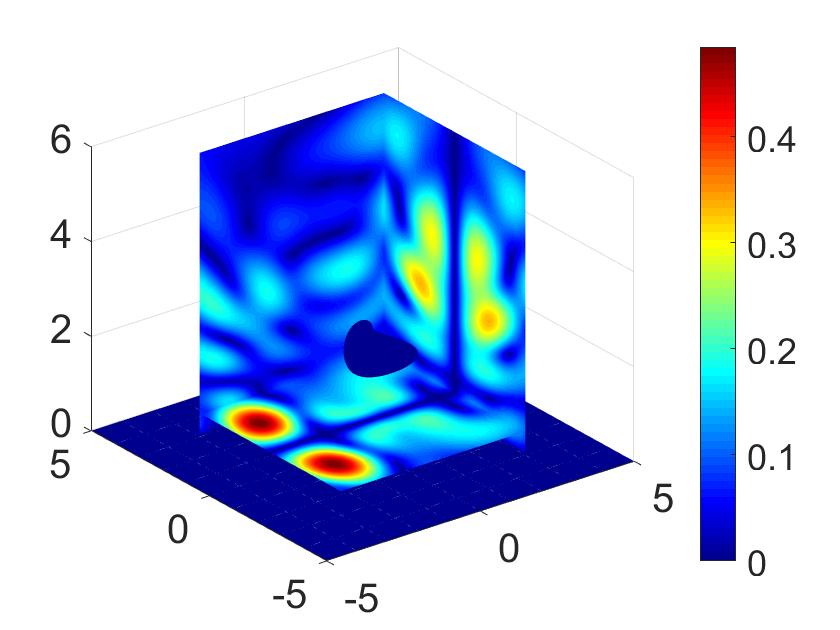
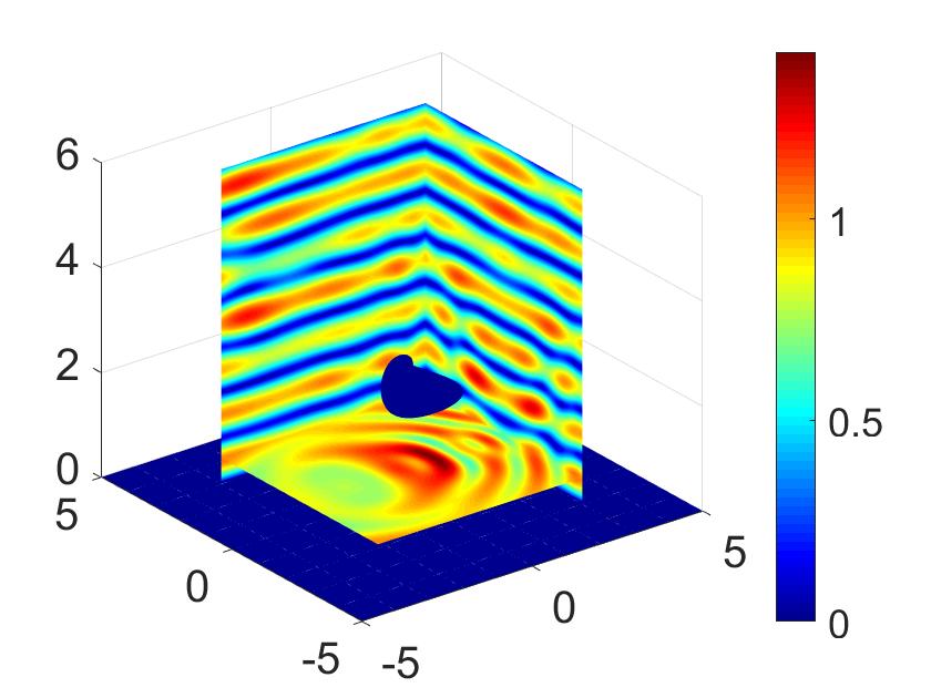
(c) $|u_{2}|$	(d) $|u_{3}|$

Figure 11: Absolute values of the three components of the total field resulting from the WGF method for the Dirichlet problem of scattering by a Bean-shaped obstacle. The section of the planar interface shown in each case coincides with the windowed region in the plane where the corresponding windowing function $\widetilde{w}_{A}$ equals to 1. $\theta^{inc}=-\pi/3$.

6 Conclusions

This paper introduced novel WGF methods for the solution of half-space elastic scattering problems with Dirichlet or Neumann boundary conditions. Relying on 1) The free-space Green function, together with 2) A novel windowed version of the classical elasticity integral equations, 3) A novel integral formulation that is uniformly accurate for all incidence angles, and 4) Efficient high-order singular-integration methods, the proposed approach avoids the expensive evaluation of the elastic layer Green function and, as demonstrated by a variety of numerical tests, can achieve uniform fast convergence for all incident angles. Extensions of the WGF approach to other types of half-space scattering problems, including e.g. fluid-solid interaction problems with multiple layers [34], Rayleigh wave scattering problems [2], and scattering problems with tapered incidence [38], etc., which can be treated by similar methods, are left for future work.

References

- [1] J. D. Achenbach, Wave Propagation in Elastic Solids, North-Holland Publishing Company: Amsterdam, 1973.
- [2] I. Arias, J.D. Achenbach, Rayleigh wave correction for the BEM analysis of elastic layer scattering problems two-dimensional elastodynamic problems in a half-space, Internat. J. Numer. Methods Engrg. 60 (2004) 2131-2146.
- [3] K. Aki, P. G. Richards, Quantitative Seismology, 2ed edition, University Science Books, Mill Valley: California, 2002.
- [4] T. Arens, The scattering of elastic waves by rough surfaces, PhD thesis, Brunel University, 2000.
- [5] T. Arens, Uniqueness for elastic wave scattering by rough surfaces, SIAM J. Math. Anal. 33 (2001) 461-476.
- [6] T. Arens, Existence of solution in elastic wave scattering by unbounded rough surfaces Math. Methods Appl. Sci. 25 (2002) 507-528.
- [7] T. Arens, T. Hohage, On radiation conditions for rough surface scattering problems, IMA J. Appl. Math. 70 (2005) 839-847.
- [8] G. Bao, L. Xu, T. Yin, Boundary integral equation methods for the elastic and thermoelastic waves in three dimensions, Comput. Method Appl. Methanics Eng. 354 (2019) 464-486.
- [9] G. Bao, T. Yin, Recent progress on the study of direct and inverse elastic scattering problems(in Chinese), Sci. Sin., Math. 47(10) (2017) 1103-1118.
- [10] O.P. Bruno, B. Delourme, Rapidly convergent two-dimensional quasi-periodic Green function throughout the spectrum-including Wood anomalies, J. Comput. Phys. 262 (2014) 262-290.
- [11] O.P. Bruno, M. Lyon, C. Pérez-Arancibia, C. Turc, Windowed Green function method for layered-media scattering, SIAM Journal on Applied Mathematics 76(5) (2016) 1871-1898.
- [12] O.P. Bruno, E. Garza, A Chebyshev-based rectangular-polar integral solver for scattering by general geometries described by non-overlapping patches, arXiv:1807.01813v1, 2018.
- [13] O.P. Bruno, E. Garza, C. Pérez-Arancibia, Windowed Green function method for nonuniform open-waveguide problems, IEEE Transactions on Antennas and Propagation 65 (2017) 4684-4692.
- [14] O.P. Bruno, L.A. Kunyansky, A fast, high-order algorithm for the solution of surface scattering problems: basic implementation, tests, and applications, J. Comput. Phys. 169(1) (2001) 80-110.
- [15] O.P. Bruno, C. Pérez-Arancibia, Windowed Green function method for the Helmholtz equation in presence of multiply layered media, Proceedings of the Royal Society A 473(2202) (2017) 20170161.
- [16] O.P. Bruno, S. P. Shipman, C. Turc, S. Venakides. Superalgebraically convergent smoothly windowed lattice sums for doubly periodic green functions in three-dimensional space, Proceedings of the Royal Society of London A: Mathematical, Physical and Engineering Sciences, 472 (2016) 2191.
- [17] O.P. Bruno, T. Yin, Regularized integral equation methods for elastic scattering problems in three dimensions, J. Comput. Phys. 410 (2020) 109350.
- [18] S. Chaillat, M. Bonnet, J.F. Semblat, A multi-level fast multipole BEM for 3-D elastodynamics in the frequency domain, Comput. Meth. Appl. Mech. Eng. 197 (2008) 4233-4249.
- [19] S. Chaillat, M. Bonnet, Recent advances on the fast multipole accelerated boundary element method for 3D time-harmonic elastodynamics, Wave Motion 50 (2013) 1090-1104.
- [20] S. Chaillat, M. Bonnet, A new Fast Multipole formulation for the elastodynamic half-space Green’s tensor, J. Comput. Phys. 258 (2014) 787-808.
- [21] A. Charalambopoulos, D. Gintides, K. Kiriaki, Radiation conditions for rough surfaces in linear elasticity, Q. J. Mech. Appl. Math. 55(3) (2002) 421-441.
- [22] J. Chaubell, O.P. Bruno, C.O. Ao, Evaluation of em-wave propagation in fully three dimensional atmospheric refractive index distributions, Radio Science 44(1) (2009) RS1012.
- [23] J. DeSanto, P.A. Martin, On the derivation of boundary integral equations for scattering by an infinite one-dimensional rough surface, J. Acous. Soc. Am. 102(1) (1997) 67.
- [24] M. Durán, E. Godoy, J.C. Nédélec, Theoretical aspects and numerical computation of the time-harmonic Green’s function for an isotropic elastic halfplane with an impedance boundary condition, ESAIM Math. Model. Numer. Anal. 44 (4) (2010) 671-692.
- [25] M. Durán, I. Muga, J.C. Nédélec, The outgoing time-harmonic elastic wave in a half-plane with free boundary, SIAM J. Appl. Math. 71(2) (2011) 443-464.
- [26] J. Elschner, G. Hu, Elastic scattering by unbounded rough surface, SIAM J. Math. Anal. 44(6) (2012) 4101-4127.
- [27] J. Elschner, G. Hu, Elastic scattering by unbounded rough surfaces: Solvability in weighted Sobolev spaces, Applicable Analysis 94 (2015) 251-278.
- [28] E. Grasso, S. Chaillat, M. Bonnet, J.F. Semblat, Application of the multi-level time-harmonic fast multipole BEM to 3-D visco-elastodynamics, Eng. Anal. Bound. Elem. 36 (2012) 744-758.
- [29] G.C. Hsiao, W. L. Wendland, Boundary Integral Equations, Applied Mathematical Sciences, Vol. 164, Springer-verlag, 2008.
- [30] G. Hu, X. Liu, F. Qu, B. Zhang, Variational approach to rough surface scattering problems with Neumann and generalized impedance boundary conditions, Communications in Mathematical Sciences 13 (2015) 511-537.
- [31] Y. Liu, Fast Multipole Boundary Element Method, Cambridge University Press, New York, 2009.
- [32] J.A. Monro. A Super-Algebraically Convergent, Windowing-Based Approach to the Evaluation of Scattering from Periodic Rough Surfaces. PhD thesis, California Institute of Technology, 2007.
- [33] J.C. Nédélec, Acoustic and Electromagnetic Equations: Integral Representations for Harmonic Problems, Springer-Verlag, New York, 2001.
- [34] D.-G. Peng, Normal Mode Acoustic Scattering Considering Elastic Layers Over a Half Space, Master thesis, Massachusetts Institute of Technology, 1997.
- [35] C. Pérez-Arancibia, Windowed integral equation methods for problems of scattering by defects and obstacles in layered media, PhD thesis, California Institute of Technology, 2016.
- [36] P.M. Shearer, Introduction to Seismology, 2nd edition, Cambridge University Press, New York, 2009.
- [37] J.W.C. Sherwood, Elastic wave propagation in a semi-infinite solid medium, Proc. Phys. Soc. 71 (1958) 207-219.
- [38] E.I. Thorsos, The validity of the Kirchhoff approximation for rough surface scattering using a Gaussian roughness spectrum, J. Acoust. Soc. Am. 83 (1988) 78-92.
- [39] T. Yin, G.C. Hsiao, L. Xu, Boundary integral equation methods for the two dimensional fluid-solid interaction problem, SIAM J. Numer. Anal. 55(5) (2017) 2361-2393.