A single-step third-order temporal discretization with Jacobian-free and Hessian-free formulations for finite difference methods

Abstract

Discrete updates of numerical partial differential equations (PDEs) rely on two branches of temporal integration. The first branch is the widely-adopted, traditionally popular approach of the method-of-lines (MOL) formulation, in which multi-stage Runge-Kutta (RK) methods have shown great success in solving ordinary differential equations (ODEs) at high-order accuracy. The clear separation between the temporal and the spatial discretizations of the governing PDEs makes the RK methods highly adaptable. In contrast, the second branch of formulation using the so-called Lax-Wendroff procedure escalates the use of tight couplings between the spatial and temporal derivatives to construct high-order approximations of temporal advancements in the Taylor series expansions. In the last two decades, modern numerical methods have explored the second route extensively and have proposed a set of computationally efficient single-stage, single-step high-order accurate algorithms. In this paper, we present an algorithmic extension of the method called the Picard integration formulation (PIF) that belongs to the second branch of the temporal updates. The extension presented in this paper furnishes ease of calculating the Jacobian and Hessian terms necessary for third-order accuracy in time.

1 Introduction

The evolution of high-performance computing (HPC) drives the advent of high-order discrete methods in computational fluid dynamics (CFD) research area. As the hardware progression of the memory capacity per compute core has become gradually saturated [1, 2], the HPC community has been compelling to find more efficient ways that can best exercise computing resources in pursuing computer simulations. Developing highly efficient numerical algorithms has become an important subject in CFD research fields. Modern practitioners have relentlessly delved into advancing high-arithmetic-intensity models that can increase numerical accuracy per degree of freedom, while at the same time, can operate with reduced memory requirements and data transfers in HPC architectures. One such computing paradigm is to promote high-order methods in which high arithmetic intensity is achieved by putting to use an increasing number of higher order terms. High-order methods (third-order or higher) avail themselves of an improved figure-of-merit in terms of reaching a target numerical error per computational time faster than the other counterpart, i.e., lower-order methods.

Within the broad framework of finite difference method (FDM) and finite volume method (FVM) discretization schemes, it has proven that high-order data interpolations and reconstructions play a key role to reduce numerical errors for solving discrete partial differential equations (PDEs) on a given grid resolution. As seen in the success of the Piecewise Parabolic Method (PPM) [3] and Weighted Essentially Non-Oscillatory (WENO) method [4], to name a few, high-order interpolation/reconstruction schemes produce more accurate numerical solutions with a faster rate of convergence-to-solution on a limited computing resource. It is of great advantage to adopting the increased intensity of floating-point operations in scientific simulations on modern HPC architecture, because otherwise increasing grid resolutions to reach the desired solution convergence will require a larger memory footprint which is typically bounded for most HPC systems.

To acquire highly accurate numerical solutions, a high-order temporal discretization scheme ought to be considered alongside the high-order spatial data interpolation/reconstruction. In the context of FDM and FVM formulations, numerical errors arise from both spatial and temporal axes since the solution lies on the spatio-temporal plane. In most compressible simulations of hyperbolic PDE systems with strong shocks, the magnitude of the maximum wave speed could most likely surpass the size of the smallest grid delta. Thus, the timestep size $\Delta t$ is typically smaller than the minimum size of grid deltas, $\min_{d=x,y,z}\{\Delta d\}$, subject to the hyperbolic CFL stability requirement. Under this condition, it is seen that the temporal error of an $m$-th order time integrator is smaller than the spatial error of an $n$-th order spatial solver, i.e., $\mathcal{O}(\Delta t^{m})<\mathcal{O}(\sum_{d=x,y,z}\Delta d^{n})$ in 3D, with the usual assumption of $m\leq n$. This, however, flips to the other end in which the temporal error becomes more dominant over the spatial error as the computational need necessitates a finer grid resolution to resolve smaller physical length scales.

For decades, the strong stability preserving Runge-Kutta (SSP-RK) time integrator [5, 6, 7] has been considered to be the standard strategy for an extensive range of high-order numerical schemes for PDE solvers. The SSP-RK schemes have proven its high fidelity which guarantees not only high-order accuracy but also numerical stability with total variation diminishing (TVD) property. The chief objective of SSP-RK schemes is to maintain the strong stability property (SSP) at high-order accuracy by sequentially applying convex combinations of the first-order forward Euler method as a building-block at each sub-stage [6]. The desired total variation diminishing (TVD) property is achieved if each of the sub-stage is TVD. The Runge-Kutta schemes pertaining this TVD property are known as SSP-RK schemes. Designed this way, the SSP-RK procedure requires $s$ multiple sub-stages to advance the solution by a single time step $\Delta t$ at $m$-th accuracy.

Of the most popular choice among various SSP-RK solvers is the three-stage, third-order RK3, given that, in practice, spatial accuracy is often considered to carry more weights than temporal accuracy in designing higher accurate spatial models [8, 9]. In contrast, devising a fourth-order SSP-RK4 is more involved to meet the favorable SSP property. Several theoretical studies have shown that a fourth-order SSP-RK4 cannot be formulated with just four sub-stages [5], meaning that the classical four-stage, fourth-order RK4 is not SSP. Other authors have demonstrated that SSP-RK4 with positive coefficients could be constructed with an increasing number of sub-stages from five up to eight [10, 11]. We remark that, to provide stable, non-oscillatory predictions in the presence of shocks, it is safer to employ SSP-RK schemes than to use non SSP-RK schemes. However, such SSP-RK schemes experience theoretical barriers in attaining the maximum available order and the maximum CFL coefficient [12, 13]. Besides, the spatial interpolation/reconstruction, as well as boundary conditions, should be applied at each sub-stage, which makes the overall procedure of SSP-RK computationally expensive. In parallel simulations, these operations also increase the footprint of data movements between node communications as the number of sub-stages grows. This very nature of SSP-RK makes it less efficient for massively parallel simulations particularly when the level of adaptive mesh refinement (AMR) progressively builds up around interesting features in simulations.

As a means of circumventing the said issues in SSP-RK, practitioners have taken a different route of providing a high-order temporal updating strategy for solving numerical PDEs. The core design principle lies in formulating a conservative temporal integrator which works for nonlinear PDEs in multiple spatial dimensions with the equivalent high-order accuracy as in SSP-RK, but, this time, in a single-stage, single-step update. The effort in this direction has resulted in what is now widely known as Arbitrary high order DERivative (ADER) method, which was first introduced in [14] for linear equations. Since then, ADER schemes have gone through several generations of breakthrough by numerous authors with the common goal of meeting the high-order requirement in a compact single-step update.

In the developments lead by Toro and his collaborators, the single-step, high-order ADER solution update is attained by solving a series of generalized (or high-order) Riemann problems (GRPs) [15, 16, 17] to compute the coefficients corresponding to the high-order terms in the power series expansion of each conservative variable in time [18, 19, 14]. Solving GRPs involves two steps. The first step is to solve one set of classical nonlinear Riemann problems for the leading term. The second step is to solve another set of classical – but linearized – Riemann problems for the rest higher derivative terms via the Cauchy-Kowalewski procedure, which exercises a sequence of full couplings between spatial and temporal derivatives.

The ADER formulation has been further taken to a more modern direction. Dumbser et al. [20] extended the original ADER scheme with multiple quadrature points to an efficient quadrature-free ADER scheme with a space-time averaged numerical flux, and the authors applied the scheme to integrate a discontinuous Galerkin (DG) solver. Balsara et al. [21] presented a new compact ADER framework that replaces the usual Cauchy-Kowalewski procedure in the original ADER formalism with a local continuous space-time Galerkin formulation up to fourth-order, and called the new approach ADER-CG (CG for continuous Galerkin). A comprehensive review on the recent developments of ADER-CG has been reported in [22]. In [23], the ADER-CG schemes are shown to be approximately twice faster than the RK methods at the same order of accuracy. It is also shown that ADER is highly adaptable to the AMR grid configuration [24]. The ADER formulation has been further extended to compressible dissipative flows in both hydrodynamics and magnetohydrodynamics in the ADER-DG framework [25] using the MOOD method [26, 27, 28, 29, 30] as a posteriori detection to enhance the shock-capturing capability; a comparison study of the space-time predictor calculation based on primitive, conservative, and characteristic variables [31]; a new approach of using the so-called automatic differentiation (or the differential transform method) to reduce the computational cost of ADER schemes called the ADER-Taylor method [32, 33, 34], etc.

Unlike the broad usage of SSP-RK in various discrete PDE solvers, the developments of ADER mentioned above have been exclusively applied to FV and DG methods, but FD methods. This is mainly because the fundamental principle of obtaining high-order accuracy in the original ADER scheme relies on solving generalized (or high-order) Riemann problems, which are the characteristic building blocks of FV and DG methods. In this regard, perhaps there could be a pathway to devise an ADER scheme for FDM within a context of a new FDM formulation called FD-Prim [35, 36, 37] in which solving Riemann problems is fully utilized as a new way of forming high-order FD fluxes.

Categorically, ODE solvers can be classified as members of multi-stage multi-derivative methods [38, 39]. For example, RK schemes are of the multi-stage type as they attain high-order accuracy via utilizing multi-stages as a primary mechanism, whereas ADER methods are of the multi-derivative type since they explore multi-derivatives as a central engine. In this paper, we are interested in constructing – for general FD solvers – a single-stage, single-step temporal updating algorithm that belongs to the class of multi-derivative methods. We follow the recent approach of the Picard integral formulation (PIF) method [40, 41] for achieving high-order temporal accuracy in FDM, where the authors designed a high-order temporal discretization by constructing a high-order approximation to the time-averaged fluxes over $[t^{n},t^{n+1}]$. The PIF discretization introduced in [40] attains third-order temporally accurate numerical fluxes by computing the coefficients of the Taylor expansion of the averaged fluxes up to third-order via the Lax-Wendroff (or Cauchy–Kowalewski) procedure which converts the high-order temporal derivatives terms in the Taylor expansion to spatial derivative terms.

As the resulting PIF scheme incorporates the needed high-order discretization directly into the numerical fluxes, the governing hyperbolic conservation law, $\partial_{t}\mathbf{U}+\nabla\cdot\mathcal{F}(\mathbf{U})=0$, can be inherently satisfied at least on a simple uniform Cartesian geometry. In contrast, in the one-step temporal discretization methods reported previously in [42, 43] for FDM, which are analogously based on the Lax-Wendroff procedure, the high-order expansion was performed on conserved variables with the Lax-Wendroff conversion of temporal derivatives to spatial derivatives. The mechanism that made these approaches conservative is set by discretizing those spatial derivatives via central differencing, which is less intrinsic than that of PIF in terms of constructing a conservative update in a discrete sense. Accordingly, in PIF, there are a few more benefits of working on the time-averaged fluxes. As shown in [41], an extra manipulation of numerical fluxes (e.g., a hybrid numerical flux as a linear combination of a low- and high-order flux to preserve positivity) does not break the hyperbolic conservation law. In addition, as will be seen throughout the present study, the high-order handling of the time-averaged fluxes can serve as an extra standalone step, apart from the rest of the conventional FDM discretization steps such as the flux splitting, high-order flux reconstruction, as well as the final temporal update. As a consequence, the PIF step can readily replace any existing SSP-RK updating step, boosting the overall performance gain by a factor of two.

The primary objective of the current work lies in providing increased flexibility and ease of computing the needed flux Jacobian and Hessian tensor terms in the original third-order PIF method [40, 41]. To do that, we offer an extended algorithmic development that permits the equivalent single-step, third-order PIF method that does not involve the analytic evaluations of the Jacobian and Hessian terms as described in [40, 41]. We call our new method a system-free PIF method (or SF-PIF in short) to reflect the added capability of the proposed Jacobian-free and Hessian-free approach.

We organize the paper as follows. In Section 2, we give an overview of the general principles in the PIF-based FD discretization. The new concept of our system-free approach to approximating the flux Jacobian and Hessian tensor terms is introduced in Section 3. We test the new SF-PIF method on a series of 1D and 2D benchmark problems in the system of the Euler equations as well as the shallow water equations. The test results are presented in Section 4. We conclude our paper with a brief summary in Section 5.

2 PIF Method

We are interested in solving the general conservation laws of hyperbolic PDEs in 1D and 2D, predicting numerical solutions with the target third-order accuracy in time. To present a mathematical foundation of our method, we begin with the following general system of equations in 2D,

$$0=\frac{\partial\mathbf{U}}{\partial t}+\nabla\cdot\mathcal{F}(\mathbf{U})=\frac{\partial\mathbf{U}}{\partial t}+\frac{\partial\mathbf{F}(\mathbf{U})}{\partial x}+\frac{\partial\mathbf{G}(\mathbf{U})}{\partial y}.$$ (1)

Denoted by $\mathbf{U}$ is a vector of conservative variables, $\mathbf{F}$ and $\mathbf{G}$ are the flux functions in $x$- and $y$- directions, respectively. Here, we apply the Picard integral formulation (PIF) [40] by taking a time average of Eq. (1) within a single timestep $\Delta t$ over an interval $[t^{n},t^{n}+\Delta t]=[t^{n},t^{n+1}]$,

$$\mathbf{U}^{n+1}=\mathbf{U}^{n}-\Delta t\left(\frac{\partial\mathbf{F}^{avg}}{\partial x}+\frac{\partial\mathbf{G}^{avg}}{\partial y}\right),$$ (2)

where $\mathbf{F}^{avg}$ and $\mathbf{G}^{avg}$ represent the time-averaged fluxes in $x$- and $y$-direction respectively,

$$\mathbf{F}^{avg}(\mathbf{x})\equiv\frac{1}{\Delta t}\int^{t^{n+1}}_{t^{n}}\mathbf{F}(\mathbf{U}(\mathbf{x},t))\mathop{dt},\quad\quad\mathbf{G}^{avg}(\mathbf{x})\equiv\frac{1}{\Delta t}\int^{t^{n+1}}_{t^{n}}\mathbf{G}(\mathbf{U}(\mathbf{x},t))\mathop{dt},\quad\quad\mathbf{x}=(x,y)\in\mathbb{R}^{2}.$$ (3)

In order to get a spatially discretized solution $\mathbf{U}_{i,j}\equiv\mathbf{U}(\mathbf{x}_{ij})$, we wish to express Eq. (2) with numerical fluxes $\hat{\mathbf{f}}$ and $\hat{\mathbf{g}}$ at cell interfaces defined as,

$$\left.\frac{\partial\mathbf{F}^{avg}}{\partial x}\right|_{\mathbf{x}=\mathbf{x}_{ij}}=\frac{1}{\Delta x}\left(\hat{\mathbf{f}}_{i+\frac{1}{2},j}-\hat{\mathbf{f}}_{i-\frac{1}{2},j}\right)+\mathcal{O}(\Delta x^{p}+\Delta t^{q}),\quad\quad\mathbf{x}_{ij}=(x_{i},y_{j}).$$ (4)

The numerical flux in $y$-direction, $\hat{\mathbf{g}}$, is defined in a similar fashion. Now we are able to express Eq. (1) in a fully discretized form as,

$$\mathbf{U}^{n+1}_{i,j}=\mathbf{U}^{n}_{i,j}-\frac{\Delta t}{\Delta x}\left(\hat{\mathbf{f}}_{i+\frac{1}{2},j}-\hat{\mathbf{f}}_{i-\frac{1}{2},j}\right)-\frac{\Delta t}{\Delta y}\left(\hat{\mathbf{g}}_{i,j+\frac{1}{2}}-\hat{\mathbf{g}}_{i,j-\frac{1}{2}}\right).$$ (5)

We remark that the derived governing form in Eq. (5) for PIF is something in between those of FVM and FDM. It is different from that of FVM that it does not carry any spatial average but the temporal average. It is also different from that of FDM that it does involve the temporal average in the fluxes in Eq. (3) to which the numerical fluxes $\hat{\mathbf{f}}$ and $\hat{\mathbf{g}}$ approximate.

We aim to get a high-order approximated solution for $\hat{\mathbf{f}}$ and $\hat{\mathbf{g}}$, both in space and time, by which the update in Eq. (5) enables us to update the solution $\mathbf{U}^{n+1}_{i,j}$ in a single step at the desired $p$-th and $q$-th accuracy in space and time. To do this, we first follow the standard convention in FDM in which we treat the pointwise $x$-flux $\mathbf{F}(x,y_{j})$ as a 1D cell average of an auxiliary function $\hat{\mathbf{F}}$ in 1D,

$$\mathbf{F}(x,y_{j})=\frac{1}{\Delta x}\int_{x-{\frac{\Delta x}{2}}}^{x+{\frac{\Delta x}{2}}}\hat{\mathbf{F}}(\xi,y_{j})d\xi.$$ (6)

Then the analytic derivative of $\mathbf{F}$ at $x=x_{i}$ in $x$-direction becomes

$$\left.\frac{\partial\mathbf{F}}{\partial x}\right|_{x=x_{i}}=\frac{1}{\Delta x}\left(\hat{\mathbf{F}}(x_{i+\frac{1}{2}},y_{j})-\hat{\mathbf{F}}(x_{i-\frac{1}{2}},y_{j})\right).$$ (7)

Comparing Eq. (7) and Eq. (4), our goal is to be achieved if we can define the numerical flux $\hat{\mathbf{f}}$ that satisfies the following relationship with $\hat{\mathbf{F}}$,

$$\hat{\mathbf{f}}_{i\pm\frac{1}{2},j}=\hat{\mathbf{F}}(x_{i\pm\frac{1}{2}},y_{j})+\mathcal{O}(\Delta x^{p}+\Delta t^{q}).$$ (8)

Mathematically speaking, the inverse problem of Eq. (6) is exactly the same as the conventional 1D reconstruction problem in FVM, the operation of which is specifically designed to find the primitive function value $\hat{\mathbf{F}}$ at a certain location (mostly, $x_{i\pm 1/2}$) in the $i$-th cell, given the integral-averaged (or volume-averaged) values ${\mathbf{F}}$ at nearby stencil points as input. Namely, this can be written as

$$\hat{\mathbf{F}}(\xi,y_{j})=\mathcal{R}\left(\mathbf{F}_{i-r,j},\dots,\mathbf{F}_{i+r,j}\right)+\mathcal{O}(\Delta x^{p}),\quad\xi\in[x_{i-\frac{1}{2}},x_{i+\frac{1}{2}}],$$ (9)

where $\mathcal{R}$ is a $p$-th order accurate reconstruction operator that takes inputs of the pointwise fluxes $\mathbf{F}$ at the $x$ neighboring stencil $[x_{i-r,j},\dots,x_{i+r,j}]$ with fixed $y=y_{j}$.

We can split the task in Eq. (8) and Eq. (9) in two different stages in the following sequential order. The first step is to attain $q$-th order temporal accuracy, followed by the second step that provides $p$-th order spatial accuracy:

1. Step 1 Approximation of the time-averaged flux – Obtain a $q$-th order approximated solution $\mathbf{F}^{appx}(\mathbf{x})$ to Eq. (3):

   $$\mathbf{F}^{avg}(\mathbf{x})\equiv\frac{1}{\Delta t}\int^{t^{n+1}}_{t^{n}}\mathbf{F}(\mathbf{U}(\mathbf{x},t))\mathop{dt}=\mathbf{F}^{appx}(\mathbf{x})+\mathcal{O}(\Delta t^{q}).$$ (10)

2. Step 2 Approximation of the high-order spatial reconstruction – Use a traditional high-order finite difference method with the approximated time-averaged fluxes $\mathbf{F}^{appx}_{i,j}$ from Step 1, instead of the conventional choice of pointwise fluxes, i.e., $\mathbf{F}_{i,j}$ at $t=t^{n}$:

   $$\hat{\mathbf{f}}_{i+\frac{1}{2},j}=\mathcal{R}\left(\mathcal{FS}\left(\mathbf{F}^{appx}_{i-r,j},\dots,\mathbf{F}^{appx}_{i+r+1,j}\right)\right)+\mathcal{O}(\Delta x^{p}).$$ (11)

   Here, $\mathcal{FS}(\cdot)$ represents a characteristic flux splitting in the positive and negative directions, and $\mathcal{R}(\cdot)$ is a high-order reconstruction scheme which is also used for FVM formulations.

In this study, we adopt the fifth-order WENO method (or WENO5) [4] for the reconstruction in Step 2, combined with the Rusanov Lax–Friedrichs flux splitting described in [9], in order to attain high-order accuracy in space domain.

Before we discuss Step 1 in details, we give a brief description on the flux splitting $\mathcal{FS}(\cdot)$, given the fact that we perform the splitting on the time-averaged approximated fluxes, $\mathbf{F}^{appx}_{\ell,j}$, $i-r\leq\ell\leq i+r+1$, whose temporal state is not at $t=t^{n}$ but at an average state over $[t^{n},t^{n+1}]$. This is different from the conventional FDM splitting which performs on the pointwise fluxes $\mathbf{F}$ at $t=t^{n}$. Following [9], the Rusanov Lax-Friedrichs splitting projects the temporally averaged fluxes $\mathbf{F}^{appx}_{\ell,j}$ from Step 1 to the left- and the right-going parts according to the characteristic decomposition of the Jacobian matrix,

$$\left.\frac{\partial\mathbf{F}}{\partial\mathbf{U}}\right|_{\mathbf{U}^{n}_{i+\frac{1}{2},j}}=\mathbf{R}_{i+\frac{1}{2},j}\Lambda_{i+\frac{1}{2},j}\mathbf{L}_{i+\frac{1}{2},j},\quad\mathbf{U}^{n}_{i+\frac{1}{2},j}=\frac{\mathbf{U}^{n}_{i,j}+\mathbf{U}^{n}_{i+1,j}}{2},$$ (12)

where $\mathbf{R}$ and $\mathbf{L}$ are the corresponding matrices of right and left eigenvectors, and $\Lambda$ is the diagonal matrix whose diagonal entries are eigenvalues. The projection proceeds to construct $s$ different left-going ($-$) and right-going ($+$) characteristic states of the averaged-fluxes, denoted as $\mathbf{V}^{k,\pm}_{(i+\frac{1}{2}):{s},j}$, to the cell interface $(i+\frac{1}{2},j)$ as

$$\mathbf{V}^{k,+}_{(i+\frac{1}{2}):{s},j}=\mathcal{FS}^{+}(\mathbf{F}^{appx}_{s,j})=\frac{1}{2}\mathbf{L}_{i+\frac{1}{2},j}^{k}\cdot\left(\mathbf{F}^{appx}_{s,j}+\alpha^{k}\mathbf{U}_{s,j}\right),\quad\mathbf{V}^{k,-}_{(i+\frac{1}{2}):{s},j}=\mathcal{FS}^{-}(\mathbf{F}^{appx}_{s^{\prime},j})=\frac{1}{2}\mathbf{L}_{i+\frac{1}{2},j}^{k}\cdot\left(\mathbf{F}^{appx}_{s^{\prime},j}-\alpha^{k}\mathbf{U}_{s^{\prime},j}\right),$$ (13)

where the sub-index $s$ ranges from $i-r,\dots,i+r$, while at the same time, $s^{\prime}=2i-s+1$. The super-index $k$ represents each characteristic field. The coefficient $\alpha^{k}$ is chosen to be the maximum absolute value of the $k$-th characteristic speed over the entire computational domain, resulting in the so-called global Lax-Friedrichs flux splitting. Here, we point out that, in conventional FDM, the temporal states of the flux and conservative vectors, the left eigenvectors, and $\alpha^{k}$ in Eq. (13) are all consistently at $t=t^{n}$. For PIF, though, the flux vector $\mathbf{F}^{appx}_{s,j}$ is at the averaged temporal state, while the others are at $t=t^{n}$. Ideally, one can also choose to compute a similar temporally averaged conservative vectors $\mathbf{U}^{appx}_{s,j}$, use them to compute $\mathbf{L}_{i+\frac{1}{2},j}^{k}$ and $\alpha^{k}$, in order to provide a consistent temporal handling across all the quantities in Eq. (13). However, we have found that the level of numerical stability as well as the solution accuracy (e.g., preserving the expected symmetries in some symmetry-preserving problems) tend to become less maintained in that approach. This observation has made us to decide that our flux splitting uses theoretically inconsistent temporal states between $\mathbf{F}^{appx}_{s,j}$ and the other quantities. As will be shown in Section 4, this treatment does not affect the overall solution accuracy and stability. The same choice has been also made in the original PIF method [40]. The rest of the flux splitting procedure follows to compute the numerical fluxes $\hat{\mathbf{f}}_{i\pm\frac{1}{2},j}$ via a high-order FDM reconstruction operator, $\mathcal{R}(\cdot)$. More specifically, we write,

$$\hat{\mathbf{f}}_{i+\frac{1}{2},j}=\sum\limits_{k}\left(\hat{\mathbf{V}}_{i+\frac{1}{2},j}^{k,+}+\hat{\mathbf{V}}_{i+\frac{1}{2},j}^{k,-}\right)\mathbf{R}^{k}_{i+\frac{1}{2},j},$$ (14)

which is a linear combination (over the $k$ characteristic fields) of the coefficients $\hat{\mathbf{V}}_{i+\frac{1}{2},j}^{k,\pm}$ obtained by solving a high-order reconstruction,

$$\hat{\mathbf{V}}_{i+\frac{1}{2},j}^{k,\pm}=\mathcal{R}\left(\mathbf{V}^{k,\pm}_{(i+\frac{1}{2}):{s},j}\right)=\mathcal{R}\left(\mathcal{FS}^{+}(\mathbf{F}^{appx}_{s,j}),\mathcal{FS}^{-}(\mathbf{F}^{appx}_{s^{\prime},j})\right),\quad s=i-r,\dots,i+r,\quad\mbox{with}\;\;\;s^{\prime}=2i-s+1.$$ (15)

In this paper we use $r=2$ for the fifth-order WENO5 method [4]. We assume that readers are familiar with the WENO5 procedure in Eq. (15); hence it is omitted in this paper. Interested readers are encouraged to refer to [4, 9].

Let us now focus on Step 1, our main interest in this study, which comprises achieving a high-order temporal accuracy of the numerical fluxes $\mathbf{F}^{appx}_{i,j}$. Traditionally, this is accomplished by a multi-stage time integrator, such as an $s$-stage, $m$-th order RK method. However, as briefly discussed in Section 1, a multi-stage method is computationally expensive, and in practice, is not suitable on an adaptive mesh refinement (AMR) grid configuration due to the increasing amount of calculation and data movements as the refinement level grows in simulations. On the other hand, by being a single-stage, single-step method, a predictor-corrector-type of time integration schemes that are based on the Lax-Wendroff (or Cauchy-Kowalewski) procedure has an advantage to reduce a plenty of computational costs and is favorable to be implemented on an AMR grid configuration while maintaining a high-order accuracy.

The PIF method is to be considered as an approach that belongs to this time integration category, featuring a new formulation of involving the concept of time-averaged fluxes. Using a time-averaged quantity in a predictor step has been widely used in FVM formulations, including the original Godunov scheme [44], piecewise-type methods [3, 45] and arbitrary derivative (ADER) schemes [18, 19, 21]. Recently, Seal et al. [40, 41] extended this approach to the FDM formulation, by way of introducing a Picard integration as described in Eq. (2), in which the time-averaged fluxes in Eq. (3) are approximated through Taylor expansion of the integrand around $t^{n}$. For example, in the third-order temporal PIF method, the time-averaged flux $\mathbf{F}^{avg}(\mathbf{x})$ is approximated by an integral of the Taylor expansion of the pointwise flux $\mathbf{F}(\mathbf{x},t)$ around $t^{n}$,

$$\begin{split}\mathbf{F}^{avg}(\mathbf{x})&=\frac{1}{\Delta t}\int^{t^{n+1}}_{t^{n}}\mathbf{F}(\mathbf{x},t)\mathop{dt}\\ &=\frac{1}{\Delta t}\int^{t^{n+1}}_{t^{n}}\left[\mathbf{F}(\mathbf{x},t^{n})+(t-t^{n})\left.\frac{\partial\mathbf{F}(\mathbf{x},t)}{\partial t}\right|_{t=t^{n}}+\frac{(t-t^{n})^{2}}{2!}\left.\frac{\partial^{2}\mathbf{F}(\mathbf{x},t)}{\partial t^{2}}\right|_{t=t^{n}}+\cdots\right]\mathop{dt}\\ &=\mathbf{F}(\mathbf{x},t^{n})+\frac{\Delta t}{2!}\left.\frac{\partial\mathbf{F}(\mathbf{x},t)}{\partial t}\right|_{t=t^{n}}+\left.\frac{\Delta t^{2}}{3!}\frac{\partial^{2}\mathbf{F}(\mathbf{x},t)}{\partial t^{2}}\right|_{t=t^{n}}+\mathcal{O}(\Delta t^{3}).\end{split}$$ (16)

Dropping the error term $\mathcal{O}(\Delta t^{3})$ in Eq. (16), we achieve a third-order temporally accurate approximation to the averaged-flux $\mathbf{F}^{avg}(\mathbf{x})$, which is what we aimed for.

The temporal derivatives can be cast in terms of spatial derivatives through the Cauchy–Kowalewski procedure, satisfying the governing system of equations. We adopt an approach conceptually slightly different from [40] to convert the temporal derivatives in Eq. (16). To wit, in [40] the temporal derivatives of the fluxes in Eq. (16) inadvertently treats $\mathbf{F}$ as a function (through $\mathbf{U}$) that depends only on $t$ but not on $\mathbf{x}$. The authors then followed a consistent logical pathway to convert the temporal derivatives to the corresponding spatial derivatives via the Cauchy-Kowalewski procedure. Although the final expression of such converted terms in [40] are found to be equivalent to our results presented below, we introduce a new self-consistent approach to converting the temporal partial derivatives in Eq. (16) to the related spatial derivatives.

To this end, we first apply the chain rule to the governing equation in Eq. (1) as,

$$\frac{\partial\mathbf{U}}{\partial\mathbf{F}}\frac{\partial\mathbf{F}}{\partial t}+\frac{\partial\mathbf{F}}{\partial x}+\frac{\partial\mathbf{G}}{\partial y}=0,$$ (17)

which leads us to write an evolution equation of the $x$-flux $\mathbf{F}$,

$$\frac{\partial\mathbf{F}}{\partial t}=-\frac{\partial\mathbf{F}}{\partial\mathbf{U}}\left(\frac{\partial\mathbf{F}}{\partial x}+\frac{\partial\mathbf{G}}{\partial y}\right),\quad\mbox{where}\quad\frac{\partial\mathbf{F}}{\partial\mathbf{U}}=\left(\frac{\partial\mathbf{U}}{\partial\mathbf{F}}\right)^{-1}.$$ (18)

From Eq. (18), the higher temporal derivatives are acquired in a successive manner. For example, the second derivative can be computed as,

$$\frac{\partial^{2}\mathbf{F}}{\partial t^{2}}=-\frac{\partial}{\partial t}\left(\frac{\partial\mathbf{F}}{\partial\mathbf{U}}\right)\cdot\left(\frac{\partial\mathbf{F}}{\partial x}+\frac{\partial\mathbf{G}}{\partial y}\right)-\frac{\partial\mathbf{F}}{\partial\mathbf{U}}\cdot\frac{\partial}{\partial t}\left(\frac{\partial\mathbf{F}}{\partial x}+\frac{\partial\mathbf{G}}{\partial y}\right),$$ (19)

where

$$\begin{split}\frac{\partial}{\partial t}\left(\frac{\partial\mathbf{F}}{\partial\mathbf{U}}\right)=\frac{\partial^{2}\mathbf{F}}{\partial\mathbf{U}^{2}}\cdot\frac{\partial\mathbf{U}}{\partial t}=-\frac{\partial^{2}\mathbf{F}}{\partial\mathbf{U}^{2}}\cdot\left(\frac{\partial\mathbf{F}}{\partial x}+\frac{\partial\mathbf{U}}{\partial y}\right),\end{split}$$ (20)

and

$$\begin{split}\frac{\partial}{\partial t}\left(\frac{\partial\mathbf{F}}{\partial x}+\frac{\partial\mathbf{G}}{\partial y}\right)&=\frac{\partial}{\partial x}\left(\frac{\partial\mathbf{F}}{\partial t}\right)+\frac{\partial}{\partial y}\left(\frac{\partial\mathbf{G}}{\partial t}\right)\\ &=\frac{\partial}{\partial x}\left(-\frac{\partial\mathbf{F}}{\partial\mathbf{U}}\cdot\left(\frac{\partial\mathbf{F}}{\partial x}+\frac{\partial\mathbf{G}}{\partial y}\right)\right)+\frac{\partial}{\partial y}\left(-\frac{\partial\mathbf{G}}{\partial\mathbf{U}}\cdot\left(\frac{\partial\mathbf{F}}{\partial x}+\frac{\partial\mathbf{G}}{\partial y}\right)\right)\\ &=-\frac{\partial^{2}\mathbf{F}}{\partial\mathbf{U}^{2}}\cdot\frac{\partial\mathbf{U}}{\partial x}\cdot\left(\frac{\partial\mathbf{F}}{\partial x}+\frac{\partial\mathbf{G}}{\partial y}\right)-\frac{\partial\mathbf{F}}{\partial\mathbf{U}}\cdot\left(\frac{\partial^{2}\mathbf{F}}{\partial x^{2}}+\frac{\partial^{2}\mathbf{G}}{\partial x\partial y}\right)\\ &\quad-\frac{\partial^{2}\mathbf{G}}{\partial\mathbf{U}^{2}}\cdot\frac{\partial\mathbf{U}}{\partial y}\cdot\left(\frac{\partial\mathbf{F}}{\partial x}+\frac{\partial\mathbf{G}}{\partial y}\right)-\frac{\partial\mathbf{G}}{\partial\mathbf{U}}\cdot\left(\frac{\partial^{2}\mathbf{F}}{\partial x\partial y}+\frac{\partial^{2}\mathbf{G}}{\partial y^{2}}\right).\end{split}$$ (21)

Here, $\frac{\partial\mathbf{F}}{\partial\mathbf{U}}$ represents an $N\times N$ flux Jacobian matrix with $\mathbf{U}\in\mathbb{R}^{N}$, while $\frac{\partial^{2}\mathbf{F}}{\partial\mathbf{U}^{2}}$ represents an $N\times N\times N$ flux Hessian tensor. A dot product between the Hessian tensor and a vector is to be understood as a tensor contraction , thus a double dot products between the Hessian tensor and two vectors, i.e., $\frac{\partial^{2}\mathbf{F}}{\partial\mathbf{U}^{2}}\cdot\left(\;\right)\cdot\left(\;\right)$, yields a vector of dimension $N$.

We approximate the spatial derivatives with the following 5-point central differencing formulae that are fourth-order,

$$\frac{\partial\mathbf{F}_{i}}{\partial x}=\frac{\mathbf{F}_{i-2}-8\mathbf{F}_{i-1}+8\mathbf{F}_{i+1}-\mathbf{F}_{i+2}}{12\Delta x}+\mathcal{O}(\Delta x^{4}),$$ (22)

$$\frac{\partial^{2}\mathbf{F}_{i}}{\partial x^{2}}=\frac{-\mathbf{F}_{i-2}+16\mathbf{F}_{i-1}-30\mathbf{F}_{i}+16\mathbf{F}_{i+1}-\mathbf{F}_{i+2}}{12\Delta x^{2}}+\mathcal{O}(\Delta x^{4}).$$ (23)

Theoretically speaking, in Eq. (16), we are able to retain the third-order temporal accuracy for $\mathbf{F}^{avg}(\mathbf{x})$ as long as we approximate ${\partial\mathbf{F}}/{\partial t}=\mathcal{O}(\Delta x^{2})$ and ${\partial^{2}\mathbf{F}}/{\partial t^{2}}=\mathcal{O}(\Delta x)$, since in a hyperbolic system the Courant condition guarantees $\Delta t=\mathcal{O}(\Delta x)$. In this regard, our design choice with the fourth-order approximations in Eqs. (22) and (23) is indeed surfeited. In addition, between Eqs. (22) and (23), it is sufficient to retain one order lower in Eq. (23) than in Eq. (22) because of the extra $\Delta t$ factor for the second derivative term in Eq. (16). In fact, in case with ${\partial^{2}\mathbf{F}_{i}}/{\partial x^{2}}=\mathcal{O}(\Delta x^{2})$, some of our test results have indicated that the convergence rate drops slightly without affecting the expected third-order solution accuracy. In practice, the use of any lower order approximation in Eq. (22) or Eq. (23) does not gain the overall computational performance; hence we stick to the fourth-order approximations.

For the cross derivatives, the simple second order central differencing is sufficient to retain the third-order temporal accuracy,

$$\frac{\partial^{2}\mathbf{F}}{\partial x\partial y}=\frac{\mathbf{F}_{i+1,j+1}-\mathbf{F}_{i-1,j+1}-\mathbf{F}_{i+1,j-1}+\mathbf{F}_{i-1j-1}}{4\Delta x\Delta y}+\mathcal{O}(\Delta x^{2},\Delta y^{2}).$$ (24)

The use of the finite central differencing formulae above leads us to approximate all the terms described in Eq. (16) with sufficient accuracy, and the time-averaged flux $\mathbf{F}^{avg}$ is ready to be reconstructed by the WENO5 method. The $y$-directional flux $\mathbf{G}^{avg}$ can be obtained in a similar way, and this finalizes the general PIF procedure introduced in [40].

What remains to discuss is the system-free methodology, an approach newly introduced in Section 3, to provide a computationally affordable and efficient strategy for Jacobian and Hessian calculations. As can be seen in [40], the straight analytical calculations of the Jacobian matrix $\frac{\partial\mathbf{F}}{\partial\mathbf{U}}$ and the Hessian tensor $\frac{\partial^{2}\mathbf{F}}{\partial\mathbf{U}^{2}}$ make hurdles to implement the PIF into a code in practice. The situation becomes even worse when extending the current method to a fourth-order or higher, in which case higher derivatives will require high dimensional tensors whose size, $N^{D}$ with $D>3$, grows dramatically. Although the Jacobian and the Hessian calculations can be easily obtained with the aid of symbolic manipulators such as SymPy, Mathematica, or Maple, it still demands complicated coding/debugging efforts and ample memory consumption. Furthermore, as the Jacobian/Hessian calculations highly depend on the type of the governing system under consideration, it is required to re-derive the Jacobian/Hessian terms analytically every time we need to solve a new system, e.g., shallow water equations, or magnetohydrodynamics (MHD) equations, to name a few.

With this in mind, in the following section, we propose a new way to attain a high-order approximation for the time-averaged fluxes without the need for direct calculation of Jacobians or Hessians. The method is to be considered as a system-free PIF method, which will be referred to as SF-PIF in what follows.

3 System-Free Approach

Our goal in this section is to provide a new alternate formulation of computing the multiplications of Jacobian-vector and Hessian-vector-vector terms in Eqs. (19) – (21). The new approach will replace the necessity for analytical derivations of these Jacobian and Hessian terms in the original PIF method that are system-dependent, with a new system-independent formulation, based on the so-called “Jacobian-free” method which is widely used for Newton-Krylov-type iterative schemes [46, 47, 48, 49]. We also extend it to a “Hessian-free” method. The resulting PIF method, called the system-free PIF (SF-PIF), approximates the Jacobian and Hessian terms via the Jacobian-free and Hessian-free approach.

3.1 Jacobian approximation

To begin with our discussion, we consider a Taylor expansion for the flux vector at a small displacement from $\mathbf{U}$,

$$\mathbf{F}(\mathbf{U}+\varepsilon\mathbf{V})=\mathbf{F}(\mathbf{U})+\varepsilon\frac{\partial\mathbf{F}}{\partial\mathbf{U}}\cdot\mathbf{V}+\frac{1}{2}\varepsilon^{2}\frac{\partial^{2}\mathbf{F}}{\partial\mathbf{U}^{2}}\cdot\mathbf{V}\cdot\mathbf{V}+\mathcal{O}(\varepsilon^{3}),$$ (25a)

$$\mathbf{F}(\mathbf{U}-\varepsilon\mathbf{V})=\mathbf{F}(\mathbf{U})-\varepsilon\frac{\partial\mathbf{F}}{\partial\mathbf{U}}\cdot\mathbf{V}+\frac{1}{2}\varepsilon^{2}\frac{\partial^{2}\mathbf{F}}{\partial\mathbf{U}^{2}}\cdot\mathbf{V}\cdot\mathbf{V}+\mathcal{O}(\varepsilon^{3}),$$ (25b)

where $\mathbf{V}$ is an arbitrary vector that has the same number of components as $\mathbf{U}$, and $\varepsilon$ is a small scalar perturbation. By subtracting Eq. (25b) from Eq. (25a), we get an expression of a central differencing that is of second-order in $\varepsilon$,

$$\frac{\partial\mathbf{F}}{\partial\mathbf{U}}\cdot\mathbf{V}=\frac{\mathbf{F}(\mathbf{U}+\varepsilon\mathbf{V})-\mathbf{F}(\mathbf{U}-\varepsilon\mathbf{V})}{2\varepsilon}+\mathcal{O}(\varepsilon^{2}).$$ (26)

Alternatively, the first-order forward differencing or the backward differencing can be used here. However, we choose the above second-order central differencing so that the order of accuracy of the entire system-free approach consistently scales with $\mathcal{O}(\varepsilon^{2})$, given that the Hessian approximation described in the next subsection is to be bounded by $\mathcal{O}(\varepsilon^{2})$. With the system-free approximation of Jacobian, all the Jacobian-vector products in Eqs. (18) – (21) are to be replaced with the central differencing in Eq. (26).

3.2 Hessian approximation

The flux Hessian tensor is unavoidable in designing the third-order PIF method in time. Below, we derive two different approximations with $\mathcal{O}(\varepsilon^{2})$ accuracy to estimate the two different types of the tensor appearing in Eqs. (19)–(21). Namely, in the first type the Hessian tensor contracts with the same vector, e.g., $\mathbf{V}$, twice, and in the second type the tensor contracts with two different vectors, e.g., $\mathbf{V}$ and $\mathbf{W}$.

For the first type, we use a Taylor expansion analogous to Eq. (25) to approximate the Hessian-vector-vector product with a central differencing of order $\mathcal{O}(\varepsilon^{2})$,

$$\frac{\partial^{2}\mathbf{F}}{\partial\mathbf{U}^{2}}\cdot\mathbf{V}\cdot\mathbf{V}=\frac{\mathbf{F}(\mathbf{U}+\varepsilon\mathbf{V})-2\mathbf{F}(\mathbf{U})+\mathbf{F}(\mathbf{U}-\varepsilon\mathbf{V})}{\varepsilon^{2}}+\mathcal{O}(\varepsilon^{2}).$$ (27)

Using a simple vector calculus, the second type can be derived from the first type in Eq. (27) by exploring a symmetric property of the Hessians,

$$\frac{\partial^{2}\mathbf{F}}{\partial\mathbf{U}^{2}}\cdot\mathbf{V}\cdot\mathbf{W}=\frac{1}{2}\left(\frac{\partial^{2}\mathbf{F}}{\partial\mathbf{U}^{2}}\cdot\left(\mathbf{V}+\mathbf{W}\right)\cdot\left(\mathbf{V}+\mathbf{W}\right)-\left(\frac{\partial^{2}\mathbf{F}}{\partial\mathbf{U}^{2}}\cdot\mathbf{V}\cdot\mathbf{V}+\frac{\partial^{2}\mathbf{F}}{\partial\mathbf{U}^{2}}\cdot\mathbf{W}\cdot\mathbf{W}\right)\right)+\mathcal{O}(\varepsilon^{2}).$$ (28)

The Hessian approximations derived here are now ready to be substituted in Eqs. (19)–(21).

3.3 Proper choices of $\varepsilon$

In the previous subsections, we approximated the Jacobian-vector product and the Hessian-vector-vector product with a small perturbation $\varepsilon$. The choice of $\varepsilon$ has to be considered carefully as it affects the solution accuracy and stability. On one hand, we need to minimize $\varepsilon$ to improve the approximated solution accuracy, the quality of which will scale as the truncation error of $\mathcal{O}(\varepsilon^{2})$. On the other hand, if it is too small the solution would be contaminated by the floating-point roundoff error which is bounded by the machine accuracy $\varepsilon_{\text{mach}}$ [47]. Therefore, $\varepsilon$ is to be determined judiciously to provide a good balance between the two types of error.

A recent study by An et al. [50] presents an effective analysis of choosing $\varepsilon$ in the context of the Jacobian-free Newton-Krylov iterative framework. The authors have shown how to compute an ideal value of $\varepsilon$ which minimizes the error of the central differencing in the Jacobian-vector approximation. We follow the same idea to obtain ideal values of $\varepsilon$ for each Jacobian-vector and Hessian-vector-vector approximation.

The main idea in [50] is to find a good balance between the truncation error $\mathcal{O}(\varepsilon^{2})$ of each Jacobian-free approximation in Eq. (26) and Hessian-free approximation in Eq. (28), and the intrinsic floating-point roundoff error $\delta\mathbf{F}(\mathbf{x})$ when calculating the target exact function value $\mathbf{F}(\mathbf{x})$ with an approximate value $\mathbf{F}(\mathbf{x})+\delta\mathbf{F}(\mathbf{x})$. The perturbation $\delta\mathbf{F}(\mathbf{x})$ may include any errors characterized in computer arithmetic such as roundoff errors, and is assumed to be bounded by the machine accuracy, i.e., $||\delta\mathbf{F}(\mathbf{x})||\leq\varepsilon_{\text{mach}}\sim 2.2204\times 10^{-16}$. In this section, we only display the outcome of this analysis which will provide a good optimal estimation of $\varepsilon$. More details of the relevant study are found in [50, 47].

Let $\varepsilon^{op}$ denote the optimal value of $\varepsilon$, and in particular, we consider computer arithmetic in a 64-bit machine with double precision. Following the analysis in [50], we obtain $\varepsilon^{op}$ for each Jacobian-free and Hessian-free approximation,

$$\begin{split}\varepsilon^{op}_{\text{jac}}&=\operatorname*{arg\,min}_{\sigma>0}\left(\frac{\sigma^{2}}{2}+\frac{\varepsilon_{\text{mach}}}{2\sigma}\right)={\left(\frac{\varepsilon_{\text{mach}}}{2}\right)}^{\frac{1}{3}}\approx$4.8062\text{\times}{10}^{-06}$,\\ \varepsilon^{op}_{\text{hes}}&=\operatorname*{arg\,min}_{\sigma>0}\left(\frac{\sigma^{2}}{3}+\frac{\varepsilon_{\text{mach}}}{\sigma^{2}}\right)={\left(3\varepsilon_{\text{mach}}\right)}^{\frac{1}{4}}\approx$1.6065\text{\times}{10}^{-4}$,\end{split}$$ (29)

where $\varepsilon^{op}_{\text{jac}}$ and $\varepsilon^{op}_{\text{hes}}$ represent the optimal $\varepsilon$ value for the Jacobian-free and Hessian-free approximations, respectively.

However, direct use of $\varepsilon^{op}$ as the displacement step size in the central differencing schemes in Eq. (26) and Eq. (28) is not a good idea for stability reasons. Usually, the vector $\mathbf{V}$ in Eq. (26) and Eq. (27) could have an enormous value in a strong shock region, so it is safer to use a smaller step size to preserve the needed stability. To meet this, we normalize the ideal value, $\varepsilon^{op}$, by the magnitude of the vector $\mathbf{V}$. There are several prescriptions available in the Jacobian-free Newton–Krylov literatures [47, 46] to help finalize our decision of choosing a proper value of $\varepsilon$ as a function of $\varepsilon^{op}$. Nonetheless, we have seen that, in a suite of test problems in Section 4, a simple approach of taking a square root of $\varepsilon^{op}$ with a simple normalization is sufficient to attain the desired accuracy and stability, which is given as,

$$\overline{\varepsilon}=\frac{\sqrt{\varepsilon^{op}}}{\left\lVert\mathbf{V}\right\rVert_{2}}.$$ (30)

Lastly, we complete the $\varepsilon$ estimation by taking the minimum value between $\overline{\varepsilon}$ and $\Delta t$,

$$\begin{split}\varepsilon=\min\left(\overline{\varepsilon},\;\Delta t\right),\end{split}$$ (31)

considering the fact that the Jacobian-free and Hessian-free terms will be multiplied by (at least) $\Delta t$ after all. As a consequence, the choice of $\varepsilon$ in Eq. (31) ensures the third-order temporal accuracy in the overall SF-PIF scheme.

4 Results

In this section, we present numerical results of the SF-PIF algorithm on a suite of well-known benchmark problems in 1D and 2D using two different systems of equations. We first demonstrate the test results of SF-PIF on the system of 1D and 2D Euler equations, and compare them with the test results of RK3 and the original PIF method. The SF-PIF is also tested on the system of 2D shallow water equations to illuminate the system-free nature of the SF-PIF algorithm.

4.1 1D Euler equations

In this section we test SF-PIF to simulate numerical problems in 1D Euler equations, defined as,

$$\frac{\partial\mathbf{U}}{\partial t}+\frac{\partial\mathbf{F}(\mathbf{U})}{\partial x}=0,$$ (32)

where the conservative variables and the corresponding fluxes are given as,

$$\mathbf{U}=\begin{bmatrix}\rho\\ \rho u\\ E\end{bmatrix},\quad\mathbf{F}(\mathbf{U})=\begin{bmatrix}\rho u\\ \rho u^{2}+p\\ u\left(E+p\right)\end{bmatrix}.$$ (33)

We adopt the spatially fifth-order WENO5 method [4] for all test problems, combined with three different time integrators: the traditional three-stage third-order Runge-Kutta method (RK3) [5], the original third-order Picard Integration Formulation (PIF) [40], and our third-order system-free PIF (SF-PIF) method presented in this paper. In all three combinations the nominal solution accuracy is expected to be fifth-order in space $\mathcal{O}(\Delta x^{5})$ and third-order in time $\mathcal{O}(\Delta t^{3})$. We use a fixed Courant number, $\text{C}_{\text{cfl}}=0.7$ in all 1D cases.

4.1.1 Sine wave advection

We start with a simple convergence test to see if the desired solution accuracy is retrieved in smooth flows. To that end, we choose a simple passive advection on a smooth flow configuration following the same setup as in [45]. The density profile is initialized with a sinusoidal wave, $\rho(x)=1.5-0.5\sin(2\pi x)$. The $x$-velocity and the pressure are set as constant values of $u=1$ and $p=1/\gamma$ with the specific heat ratio, $\gamma=5/3$. Albeit solved using the nonlinear Euler equations, the problem is solved in a linear regime, viz., the velocity and pressure remain constant for all $t\geq 0$ so that the initial sinusoidal density profile is purely advected by the constant velocity $u=1$ without any nonlinear dynamics such as a formation of shocks and rarefactions.

The simulation domain is defined on an interval $[0,1]$ with the periodic boundary condition on the both ends. The density profile will propagate for one period through the simulation domain and will return to its initial position at $t=1$. On return, by being a linear problem, any deformation of the density profile from the initial shape can be considered as a numerical error associated with phase errors or numerical diffusions. The accuracy of the numerical solutions is measured by computing the $L_{1}$ error between the solution at $t=1$ and the initial profile on a different number of cells $N_{x}=32,64,128,256,512$ and $1024$. The results are depicted in Fig. 1 for all three different temporal integrating schemes, RK3, PIF, and SF-PIF.

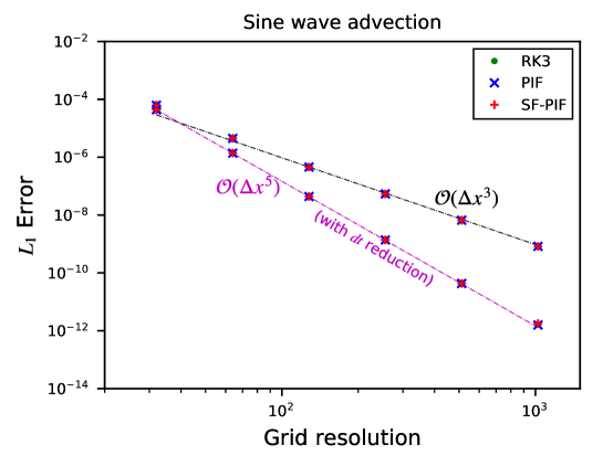
Figure 1: Convergence test for the 1D sine wave advection problem. The errors are calculated in $L_{1}$ sense against the initial density profile resolved on the computational grids refined from 32 to 1024 by a factor of 2. All numerical solutions follow the theoretical third-order convergence rate (the black-dotted line) when using the timesteps computed from the Courant condition. Also plotted are the solutions of using reduced timesteps, which follows the fifth-order convergence rate represented in the pink-dotted line.

There are two types of result demonstrated in Fig. 1. In the first type, the discrete solutions of three different temporal schemes advanced with timesteps computed from the Courant condition with $C_{\text{cfl}}=0.7$. Interestingly, we observe that the numerical solutions from SF-PIF as well as the other two schemes converge at third-order, indicating that the overall leading error of the simulation is dominated by the third-order accuracy of the temporal schemes despite the use of the more accurate fifth-order spatial WENO5 solver. As also briefly mentioned in Section 1, at low-mid resolutions, solution accuracy of simulations is mostly governed by the spatial accuracy until the leading error of the solution is caught up by the temporal error as computational grids get further refined to higher resolutions. So, in this problem, one may expect that the numerical solutions would pick up a faster convergence, faster than third-order and closer to fifth-order, at least at the lower end of the grid resolutions. Unfortunately, this doesn’t happen in this test and the third-order temporal accuracy quickly takes over the control throughout the entire range of the grid resolutions tested herein. This solution behavior supports strongly the importance of integrating spatially interpolated/reconstructed solutions with a temporal scheme whose accuracy is sufficiently high enough to be well comparable to that of the spatial solver.

In the second type, however, timesteps are restricted in order to match up the lower third-order temporal accuracy of $\mathcal{O}(\Delta t^{3})$ with the higher fifth-order spatial accuracy of $\mathcal{O}(\Delta x^{5})$ . We follow the usual trick of timestep reduction (e.g., see [9]) to manually adjust the timestep $\Delta t_{N}$ on a grid size of $N$ to an adjusted value, satisfying the equal rate of change between the spatial and temporal variations. As a result, the restricted (or reduced) timestep is defined by,

$${\Delta t_{N}}={\Delta t_{0}}\Big{(}\frac{\Delta x_{N}}{\Delta x_{0}}\Big{)}^{\frac{5}{3}}.$$ (34)

The sub-indices “$0$” and “$N$” refer to the time and grid scales on a nominal coarse and a fine resolution, respectively. For instance, in the current configuration, $\Delta x_{0}$ is the grid scale on $N_{x}=32$ and $\Delta t_{0}$ is the corresponding timestep subject to the Courant condition with $C_{\text{cfl}}=0.7$. With the reduction, the overall leading error of the simulation (from both spatial and temporal) is matched with the fifth-order spatial accuracy of WENO5, and the numerical solution of SF-PIF follows the fifth-order rate as expected. Moreover, the SF-PIF solution compares indistinctly well with the other two solutions, almost in the same pattern. Even though the timestep reduction helps improve the numerical convergence rate, particularly when a temporal solver has a lower accuracy than a spatial solver, such simulations suffer not only from a much longer computational time to reach a target final time $t=t_{\max}$ but also from a degradation of solution effectiveness in resolving small scales due to an extended simulation time [51, 52].

In all cases, the solution of SF-PIF compares equally well with the solutions of the original PIF and RK3 in both quantitatively and qualitatively.

4.1.2 Sod’s shock tube problem

The Sod’s shock tube problem [53] is the one of the most famous hydrodynamics test problems for testing a numerical scheme’s capability to handle discontinuities and shocks. The initial condition is given as,

$$\left(\rho,u,p\right)=\begin{cases}\left(1,0,1\right)&\text{for }x\leq 0.5,\\ \left(0.125,0,0.1\right)&\text{for }x>0.5,\end{cases}$$ (35)

in a simulation box of $[0,1]$, with outflow boundary conditions on both ends at $x=0$ and $x=1$.

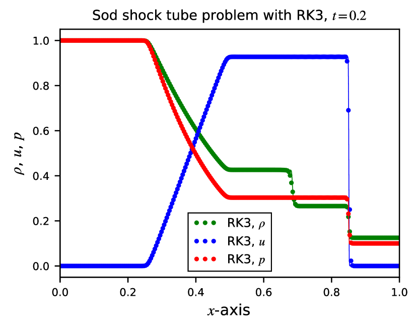
(a)

(b)

(c)

Figure 2: Sod’s shock tube problem at $t=0.2$. The reference solutions are over-plotted as solid lines in each panel, which are resolved on a grid resolution of $N_{x}=1024$ with RK3. The symbols in each panel represent the solution resolved on $N_{x}=256$ grid cells with (2(a)) RK3, (2(b)) PIF, and (2(c)) SF-PIF.

The results with the grid size of $N_{x}=256$ at $t=0.2$ are plotted as symbols in Fig. 2. The solid lines on each panel represent the reference solution resolved on a more finer grid size, $N_{x}=1024$, by using WENO5+RK3. As seen in Fig. 2, the solutions of SF-PIF agree with the reference solution and the two solutions from RK3 and PIF. We see that, in PIF and SF-PIF, there is a slight oscillation in the $x$-velocity immediately behind the shock front. We believe that this small oscillation is originated from the use of the central differencing formulae in Eqs. (22) – (24) for both SF-PIF and PIF. Even though we haven’t found any test case in our numerical experiments that this oscillatory prediction negatively impacts the overall performance of the SF-PIF scheme, this could potentially degrade the capability of shock/discontinuity handling in SF-PIF in more extreme problems. As such, this issue will be investigated further in our future studies.

4.1.3 Two-blast wave

Since originally introduced by Woodward and Colella [54], this test problem has been chosen by many practitioners to examine codes’ capability of capturing the correct dynamics of shock-shock interactions. Initially, two strong shocks are developed at each end of the simulation box $\left[0,1\right]$. The reflecting boundary conditions are used at both ends, $x=0$ and $x=1$. They are driven to each other, leading to a highly compressive collision at the middle part of the domain at $t\sim 0.028$ by the initial pressure discontinuities. The shock-shock collision produces an extremely high and narrow density peak. One of the main points of interest is to demonstrate how well numerical solutions predict the density profile and its peak amplitude particularly at $t=0.038$, one hundredth of a second after the strong collision.

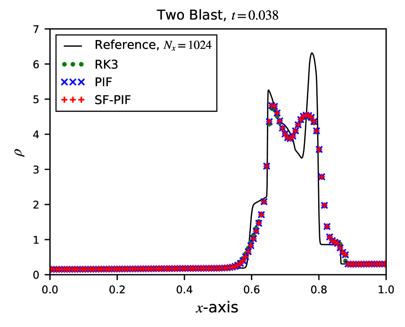
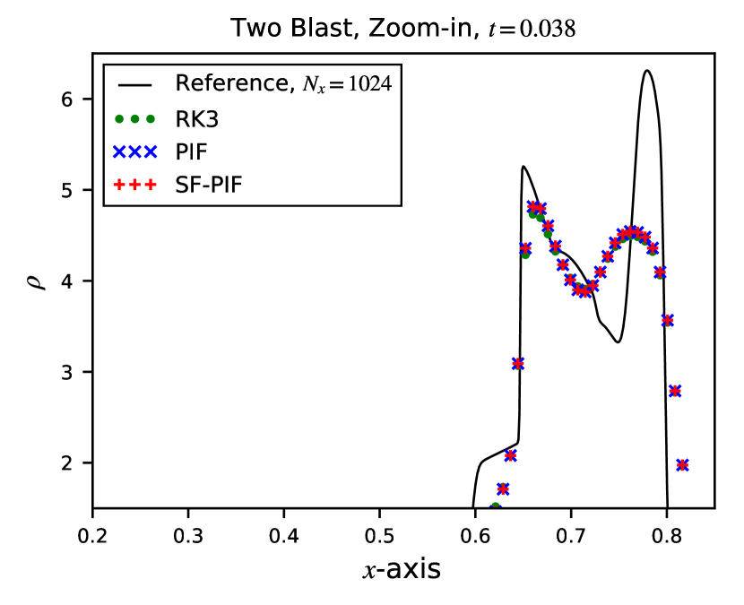
Figure 3: Two-blast wave problem at $t=0.038$. The symbols depict the numerical solutions resolved on a resolution of $N_{x}=128$, and the solid line represents the reference solution on a finer grid, $N_{x}=1024$, with RK3 method. Right: A close-up view of the shock interaction region.

In Fig. 3, the density profile with SF-PIF is plotted against two other density profiles with RK3 and PIF on a grid resolution of $N_{x}=128$. Over-plotted is the reference solution (the black solid curve) integrated with RK3 on a grid size $N_{x}=1024$ for comparison. We see that all three methods produce an acceptable quality of solutions and they are all in good agreement. As observed in the close-up view in the right panel of Fig. 3, there are slight improvements in the solutions of SF-PIF and PIF over the RK3 solution in resolving the peak density amplitudes following the sharp gradients over $0.63\leq x\leq 0.8$. It is not surprising to see that the two solutions are nigh equivalent since the two methods share the same common ground in mathematical formulation. On the other hand, the equivalency of the two methods affirms that our system-free approach described in Section 3 not only provides ease of code implementation but also guarantees high fidelity in solution accuracy compared against the analytical approach of the original PIF method.

4.1.4 Shu-Osher problem

The Shu-Osher problem [55] describes an interaction of a Mach 3 shock and a smooth density profile. Initially, a right-going Mach 3 shock propagates into the low density profile with sinusoidal perturbations. As the shock proceeds, it is superposed with the sinusoidal density profile, leaving two different trails of density behind the right-propagating shock.

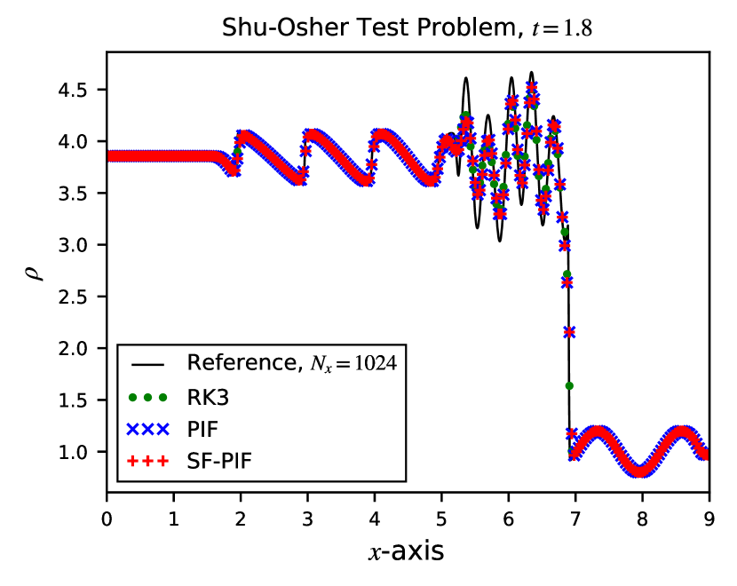
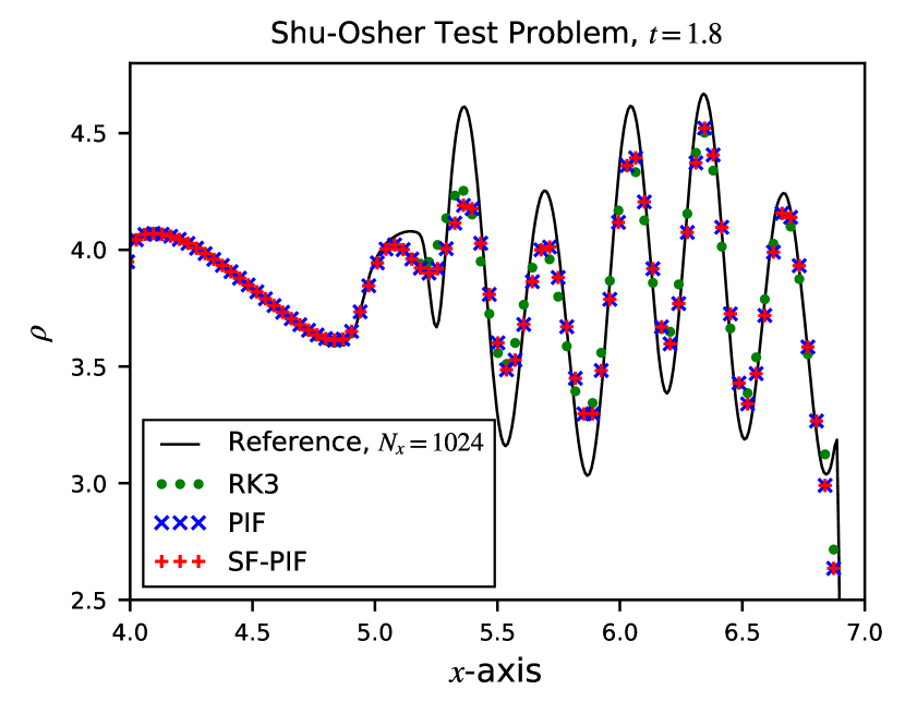
Figure 4: The Shu-Osher test problem at $t=1.8$. The reference solution, plotted as a black solid curve, is obtained on $N_{x}=1024$ grid resolution with RK3 method. Other solutions are resolved on $N_{x}=256$ grid resolution, represented as symbols. Right: A close-up view of the doubled frequency region to illustrate methods’ numerical diffusivity.

The initial sine wave gets compressed by the penetrating shock, doubling the perturbation frequency in the downstream of the immediate post-shock region. From the tail of the high frequency region to the farther left, the perturbation returns to the original frequency, but at the same time, the profile experiences a shock-steepening which leads the initial smooth profile into a sequence of sharp density gradients further away to the downstream.

Our main focus on this test problem is to check whether the SF-PIF scheme is able to advance the discrete solutions in a stable and accurate manner, capturing both the smooth and discontinuous profiles in the double-frequency region as well as at the shock front. Fig. 4 shows the SF-PIF result at $t=1.8$ with the other two methods of RK3 and PIF. All three results are resolved on $N_{x}=256$ grid cells, while the reference solution is obtained on a much higher resolution of $N_{x}=1024$ with RK3 method, displayed in a black solid curve. The results illustrated in the close-up view on the right show that the two single-stage methods, SF-PIF and PIF, are able to produce density peak amplitudes in the double-frequency region slightly higher than the solution from the multi-stage RK3 method. As before, the two solutions of SF-PIF and PIF are found to be almost indistinguishable, assuring the validity of the system-free formulations of the Jacobian and Hessian terms in SF-PIF compared with the analytic calculations of the same terms in the original PIF scheme.

4.2 2D Euler equations

In this section, we implement the SF-PIF scheme to solve the two-dimensional Euler equations, defined by Eq. (1) with,

$$\mathbf{U}=\begin{bmatrix}\rho\\ \rho u\\ \rho v\\ E\end{bmatrix},\quad\mathbf{F}(\mathbf{U})=\begin{bmatrix}\rho u\\ \rho u^{2}+p\\ \rho uv\\ u\left(E+p\right)\end{bmatrix},\quad\mathbf{G}(\mathbf{U})=\begin{bmatrix}\rho v\\ \rho uv\\ \rho v^{2}+p\\ v\left(E+p\right)\end{bmatrix}.$$ (36)

As before, WENO5 is used as the spatial method in all 2D test problems in this section so that we can focus on differing numerical effects only from the temporal methods. We present results from several 2D test problems and compare them to address the performance of the SF-PIF scheme. We choose the CFL number $C_{\text{cfl}}=0.4$ in all problems.

4.2.1 Nonlinear isentropic vortex advection

Our first 2D problem considers SF-PIF’s accuracy and speedup in two-dimensional Euler equations. We conduct the nonlinear isentropic vortex advection problem originally introduced by Shu [56]. Here, we modify the problem as presented in [57] where the size of the periodic domain $[0,20]\times[0,20]$ is twice larger in each direction than the original setup in [56] to prevent self-interactions of the vortex across the periodic domain. The same consideration was also found in [45, 37]. Initially positioned at the center of the domain, the isentropic vortex starts to advect in the positive diagonal direction and returns to the initial location after one periodic time, $t=20$. The $L_{1}$ error is calculated through the direct comparison between the initial condition and the numerical solution at $t=20$ to examine numerical convergence rates on four different grid resolutions, $N_{x}=N_{y}=50,100,200$, and $400$.

Table 1: The $L_{1}$ errors, the rates of convergence, and the relative computation times for the vortex advection test. Here, we display the comparison between RK3 and SF-PIF only since the difference between SF-PIF and PIF is indistinguishable.

$N_{x}=N_{y}$	RK3				SF-PIF
	$L_{1}$ error	$L_{1}$ order	Speedup		$L_{1}$ error	$L_{1}$ order	Speedup
50	$7.22\text{\times}{10}^{-1}$	–	1.0		$6.95\text{\times}{10}^{-1}$	–	0.64
100	$5.76\text{\times}{10}^{-2}$	3.65	1.0		$5.58\text{\times}{10}^{-2}$	3.64	0.56
200	$2.94\text{\times}{10}^{-3}$	4.29	1.0		$2.89\text{\times}{10}^{-3}$	4.27	0.56
400	$1.22\text{\times}{10}^{-4}$	4.59	1.0		$1.26\text{\times}{10}^{-4}$	4.52	0.51

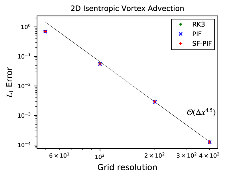
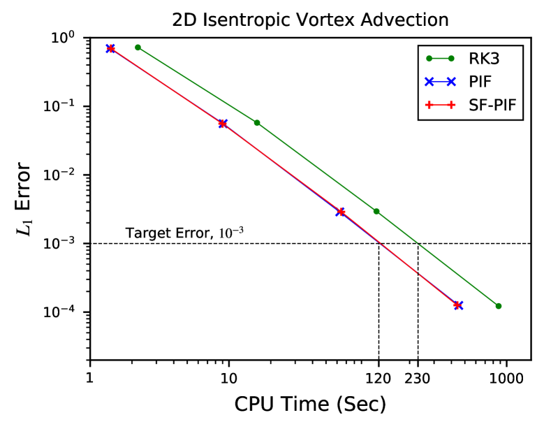
Figure 5: Left: The $L_{1}$ errors of the isentropic vortex advection problem with respect to the grid resolutions, $50,100,200,$ and $400$. All simulations use WENO5 for spatial reconstruction with CFL=0.4. Right: The $L_{1}$ errors of the isentropic vortex advection problem as a function of computational time.

The results of the convergence test are summarized in Table 1 and depicted on the left panel in Fig. 5. We see a good comparable match in magnitudes of the $L_{1}$ errors across all three methods. Between SF-PIF and PIF, there is no significant distinction in their accuracy and performance, as demonstrated on both panels in Fig. 5. All three methods converge at 4.5th order towards the initial condition at each grid resolution. Unlike the 1D linear sine advection test in Section 4.1.1, we do not see the full dominance in error from the third-order temporal discretization (at least over the range of the grid resolutions tested herein), which could potentially reduce the overall convergence rate down to third-order as in the sine advection case. Concurrently, we also see that the solution does not converge at full fifth-order either, the rate of which is due from the use of WENO5. This can be explained as a nonlinear effect in which the overall leading error term of the fifth-order spatial discretization is slightly compromised by the lower third-order time integration schemes. In general, an exact analysis of this phenomenon is highly problem dependent and it often becomes intractable in many nonlinear cases. In practice though, this issue can be improved by one of the two approaches, timestep reductions, or developments of fourth-order or higher temporal methods. As discussed, the first option is not favorable in most large-scale simulations, and hence the latter is to be considered as a better alternative from the mathematical standing point.

On the right panel, we illustrate the performance of SF-PIF measured in terms of the CPU time to reach a target error threshold, say $L_{1}$ error of $10^{-3}$. As demonstrated, the results of the two single-stage methods, SF-PIF and PIF, coincide to each other and their performance is approximately twice faster than the multi-stage method of RK3. It is worth to be noted that the SF-PIF approach can be readily swappable with an RK integrator in an existing code without too much effort, leaving any existing spatial implementations intact mostly. Moreover, such a code transformation with SF-PIF is more advantageous in simplicity than with the original PIF method because SF-PIF replaces PIF’s need for analytic derivations of the Jacobian and Hessian terms with the system-free approximations, which have shown to be highly commensurate with the analytical counterparts of the PIF scheme.

4.2.2 2D Riemann problems

Next, we consider 2D Riemann problems which are extensively studied in [58, 59, 60] and widely used for the code verifications [45, 61, 62, 63, 37]. Among a wide range of different configurations, we demonstrate two test cases, Configuration 3 and Configuration 5, following the descriptions in [63, 45]. Both test cases are resolved on a square simulation box of $\left[0,1\right]\times\left[0,1\right]$ with $400\times 400$ grid cells using outflow boundary conditions.

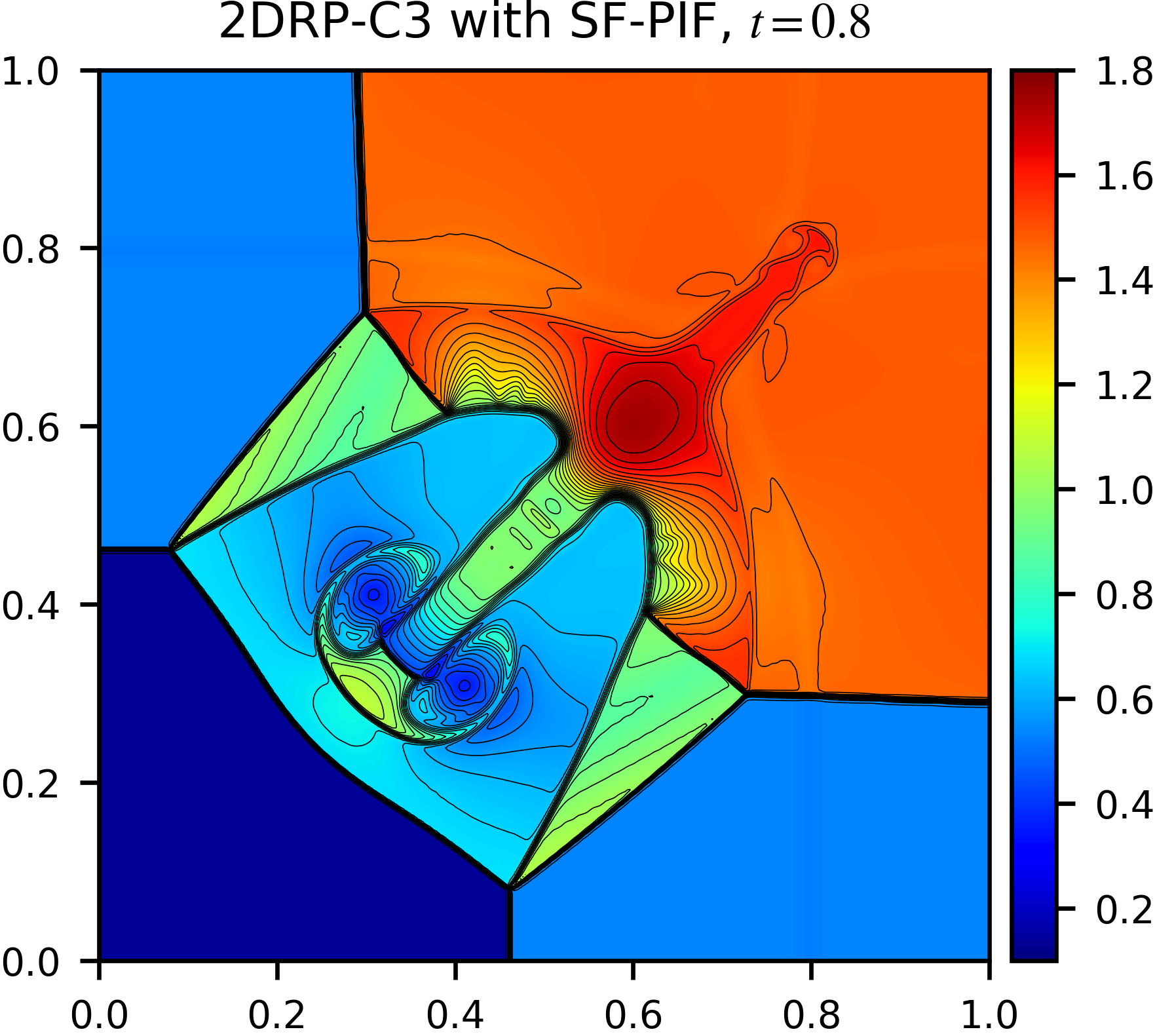
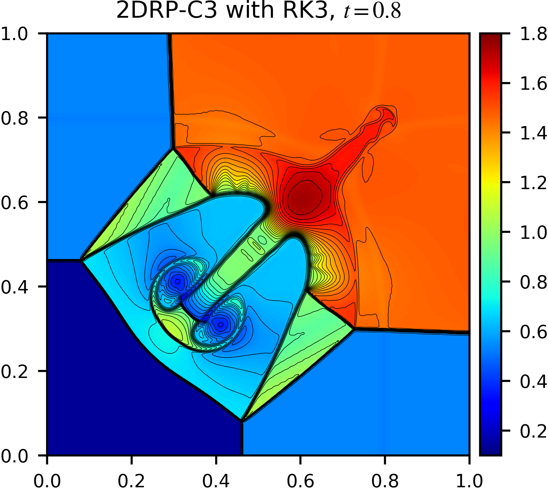
Figure 6: The density profile of Configuration 3 with SF-PIF (left) and with RK3 (right). The color map ranges from $0.1$ to $1.8$, and 40 evenly-spaced contour lines are over-plotted with the same range.

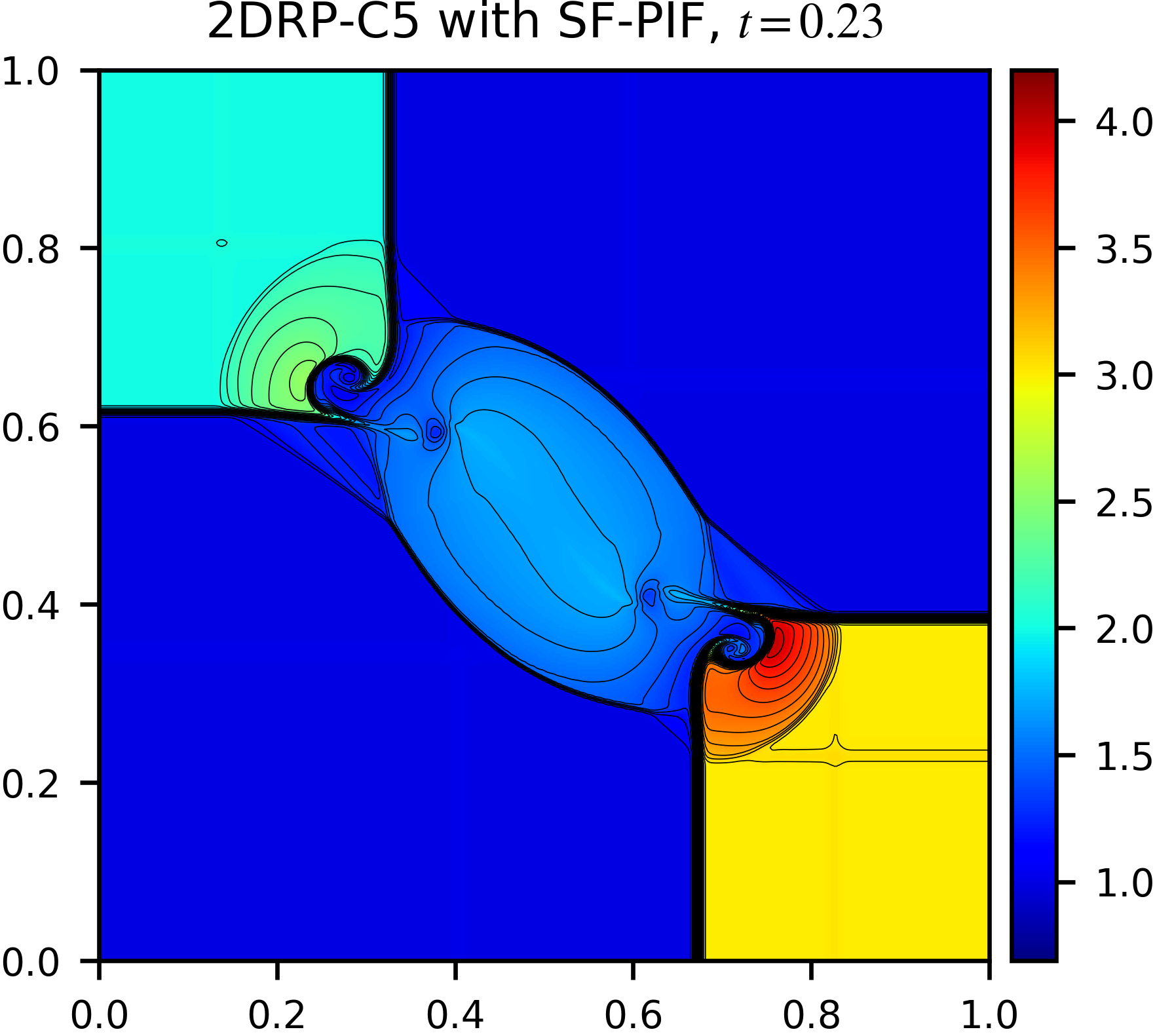
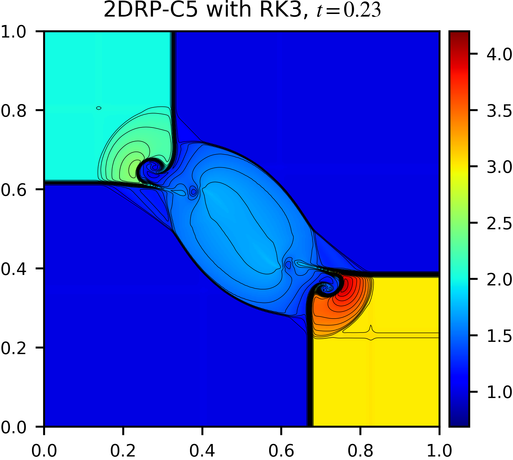
Figure 7: The density profile of Configuration 5 with SF-PIF (left) and with RK3 (right). The color map ranges from $0.69$ to $4.2$, and 40 evenly-spaced contour lines are over-plotted with the same range.

The results of Configuration 3 and Configuration 5 are shown in Fig. 6 and Fig. 7, respectively. The density maps are visualized with pseudo-color schemes ranging between 0.1 and 1.8 in Configuration 3, and between 0.69 and 4.2 in Configuration 5. Over-plotted are 40 levels of contour lines using the same density range in each configuration.

We see that the SF-PIF result is well comparable to that of RK3, which assures that SP-PIF method is eminently reliable in temporally advancing solutions with discontinuities and shocks in 2D, while at the same time, preserving the expected symmetries and flow profiles in each problem. In both, however, there is yet no formation of secondary Kelvin-Helmoltz instabilities, typically exhibited as vortical rollups along the slip lines – the regions connecting the inner edges of the triangle “arms” surrounding the mushroom-jet and the stem of the mushroom-jet. Direct comparisons with other FDM test results on the same grid resolution with comparable accuracy (e.g., Fig. 12 in [37]; Fig. 6 in [63]) reveal that their test results have more pronounced rollup structures developed along the slip lines. This implies that both of the test results here have more numerical diffusivity than those approaches therein [63, 37]. We first emphasize that developments of small-scale features relevant to grid scales depend much more sensitively on the choice of spatial solvers (e.g., WENO5 with the global Rusanov flux-splitting in our case), but less on a temporal solver. It is well-known that the global Rusanov flux-splitting (used in this study but not in [63, 37]) has added numerical diffusivity, which can delay an onset of the secondary instability formation in our experiments. Secondly, with mathematical rigor, an increasing number of rollups in any given scheme should only be understood as a proof of a less amount of numerical dissipation, but not as a proof of a better numerical method, than others. Measuring a proper amount of such rollups in any given simulations on a set of specific setups (i.e., grid resolutions, spatial and temporal orders of numerical methods, parameters, etc.) is not a simple task. Such a study will need to involve an extensive systemic comparison analysis that requires careful validation and verification tests, the topics of which are beyond the scope of this paper.

4.2.3 Implosion test

The next problem to consider is the implosion test problem introduced by Hui et al. [64]. An unsteady flow configuration is given as an initial condition which launches a converging shock wave towards the domain center. We follow a simpler version by Liska and Wendroff [65], which takes only the right upper quadrant of the original setup in [64] as the simulation domain. In this setup, the simulation is initialized on a region of a square domain, $\left[0,0.3\right]\times\left[0,0.3\right]$, enclosed with reflecting walls, in which case a converging shock wave is launched toward the lower left corner at $(x,y)=(0,0)$. The initial shock wave gets bounced by the reflecting walls and produces a double Mach reflection along two edges of $x=0$ and $y=0$. As a consequence, two jets are formed along the edges moving toward the origin $(x,y)=(0,0)$ and collide each other. This two-jet collision then ejects a newly-formed jet into the diagonal direction $x=y$. Reflecting shocks continuously interact with the diagonal jet, turning it into a longer and narrower shape over time. The observed structures of filaments and fingers along the diagonal jet and at its base are progressively intensified by the Ritchmyer-Meshkov instability, a level of which depends sensitively on numerical dissipation. The shape of the jet is the key view point of the implosion test since it is a good indicator of a code’s symmetric property and numerical dissipation. If the numerical scheme fails to maintain a high level of symmetry, the jet will eventually be derailed off-diagonally and deformed over time. Besides, an excess amount of numerical dissipation will turn the jet into a less narrow and less elongated shape along the diagonal.

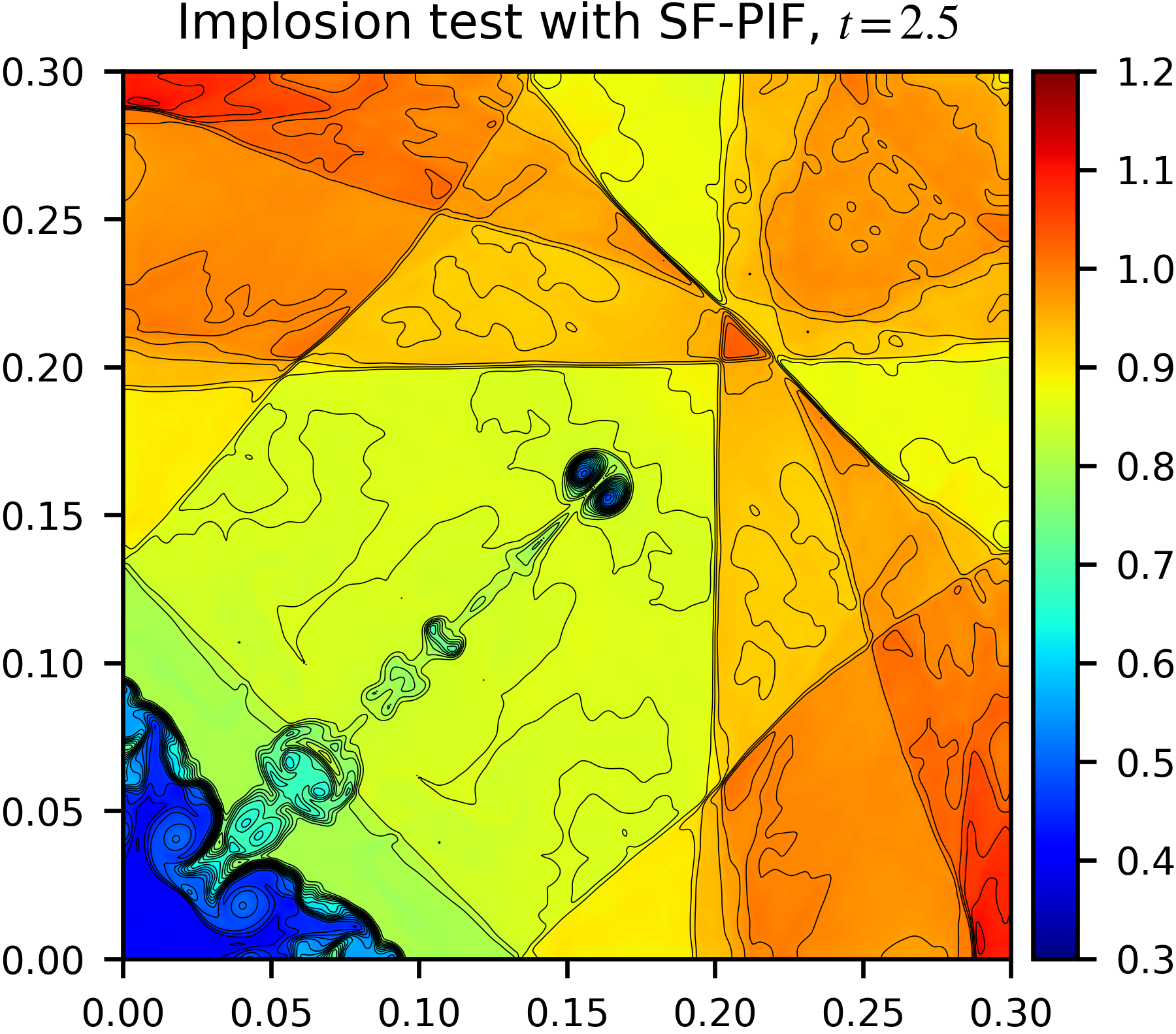
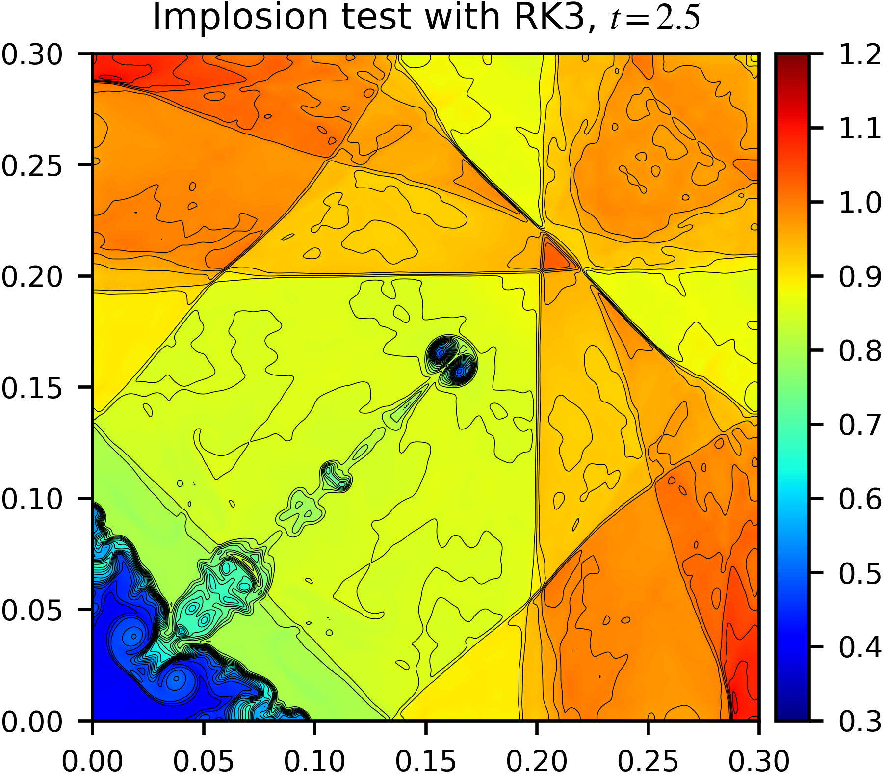
Figure 8: The density profile of the implosion test with SF-PIF (left) and with RK3 (right). The color map ranges from $0.3$ to $1.2$, and 40 evenly-spaced contour lines are over-plotted with the same range.

We display our results on a $400\times 400$ grid resolution at $t=2.5$. The result with SF-PIF is on the left panel in Fig. 8 and RK3 on the right. These results can also be directly compared with Fig. 4.7 in [65] and Fig. 17 in [66]. We clearly see that the contour lines of SF-PIF (as well as RK3) are shown to retain the diagonal symmetry at a highly sufficient level. At the same time, the shape of the diagonal jet using SF-PIF matches well with the shape using RK3, and hence is suffice to demonstrate that the numerical dissipation in SF-PIF is well-managed compared with RK3.

4.2.4 Double Mach reflection

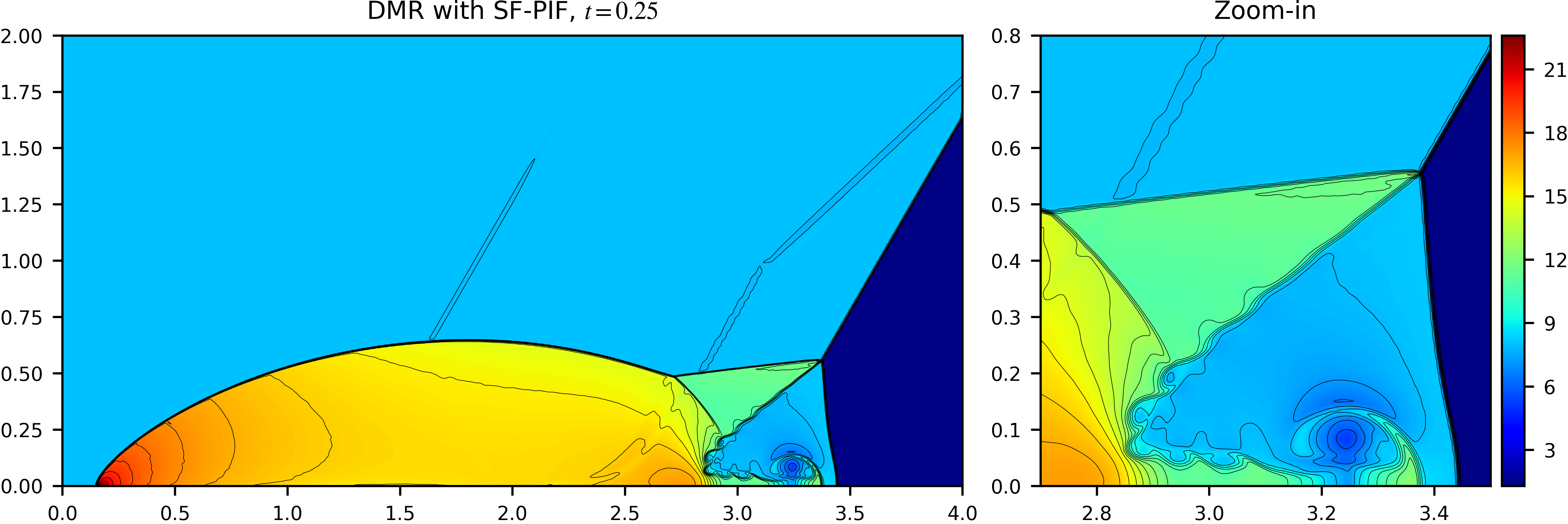
Figure 9: Left column: The density profile of the double Mach reflection (DMR) problem solved with SF-PIF (top) and RK3 (bottom). Right column: Close-up views near the triple-point of the density profile. The contour lines display 30 linearly separated points. All plots use the same range of density, $[1.3,22.6]$. All calculations are conducted on a grid resolution of $1024\times 512$ with $C_{\text{cfl}}=0.4$.

Our last test using the Euler equations in 2D is the double Mach reflection problem introduced by Woodward and Colella [54]. We follow the original setup except that we doubled the domain size in the $y-$direction to avoid any disturbances by the numerical artifacts from the top boundary [67]. A Mach 10 planar shock is initialized at the left side of the domain with a $30^{\circ}$ angle to the reflecting bottom surface. As the shock propagates to the right, the bottom wall continuously bounces off the shock wave and creates a round reflected shock. The solution further evolves into forming two contact discontinuities and two Mach stems, as well as a jet along the bottom surface. The formation of this jet is similar to the formation of the two jets in the previous implosion test, the collision of which led to the upward moving diagonal jet.

The main point of discussion is to observe the appearance of the contact discontinuity that spans from the triple-point at $(x,y)\approx(3.38,5.5)$ in Fig. 9 to the dense jet along the bottom wall, displayed in the panels on the right column in Fig. 9. A lower amount of numerical dissipation in a scheme makes this region more susceptible to Kelvin-Helmholtz instability, leading to an onset of vortical roll-ups along the slip line. Henceforth, the amount of such roll-ups serves as an indicator of the scheme’s numerical diffusivity. As discussed in the 2D Riemann problems in Section 4.2.2, we once more point out that such an assessment should only be used to address each scheme’s numerical diffusivity, but not to be used to rank different schemes without careful validation and verification studies.

The density results are represented in Fig. 9, and the detailed views are shown in the right panel. Shown in the top row in Fig. 9 is the density profile integrated using SF-PIF in the range of $[1.3,22.6]$ at $t=0.25$, computed on a grid resolution of $1024\times 512$. We also plot 30 evenly spaced contour lines of density in the same range. The result with RK3 is in the bottom row. We can see that the time prediction of density using SF-PIF matches sufficiently well with the result using RK3, confirming the validity of SF-PIF in comparison.

4.3 Shallow water equations

In this section, we switch the governing equations to a system of 2D shallow water equations (SWE) without a source term, defined by a conservative hyperbolic system as,

$$\mathbf{U}=\begin{bmatrix}h\\ hu\\ hv\end{bmatrix},\quad\mathbf{F}(\mathbf{U})=\begin{bmatrix}hu\\ hu^{2}+\frac{1}{2}gh^{2}\\ huv\end{bmatrix},\quad\mathbf{G}(\mathbf{U})=\begin{bmatrix}hv\\ huv\\ hv^{2}+\frac{1}{2}gh^{2}\end{bmatrix}.$$ (37)

Here, $h$ is the vertical depth of the fluid, $\mathbf{v}=\left(u,v\right)$ is a vector of vertically-averaged velocity components in $x$ and $y$ directions. Denoted as $g$ is a gravitational acceleration in the negative vertical $z$ direction, which is averaged out in the derivation of the shallow water equations.

The sole purpose of presenting this new system of equations is to demonstrate the flexibility of our SF-PIF scheme, in that the system-free approach allows an easy code implementation without the need for another analytical calculation of new Jacobian and Hessian terms of the new governing system. By the system-independent property of the SF-PIF method, the process of changing from the 2D Euler code to the 2D SWE code is no more than switching the governing equations. This process is much simpler than what is needed in the original PIF method, enabling the overall code transition is highly smooth and transparent without any extra effort to modify a substantial portion of code lines.

We conduct a simple circular dam breaking simulation, which has been widely adopted for code validation purposes in many SWE literatures [68, 69, 70]. Initially, a volume of still water is confined in the virtual (i.e., invisible) cylindrical wall with a radius of 11 meters (m), located at the center of simulation domain, $\left[$50\text{\,}\mathrm{m}$\times$50\text{\,}\mathrm{m}$\right]$. The depth of the water inside of the wall is $10\text{\,}\mathrm{m}$ and $1\text{\,}\mathrm{m}$ outside. This configuration would be considered as an SWE version of 2D Riemann problem. Explicitly, the initial condition is given as,

$$\left(h,u,v\right)=\begin{cases}\left($10\text{\,}\mathrm{m}$,0,0\right)&\text{for }r\leq$11\text{\,}\mathrm{m}$,\\ \left($1\text{\,}\mathrm{m}$,0,0\right)&\text{for }r>$11\text{\,}\mathrm{m}$,\\ \end{cases}$$ (38)

where $r$ is the distance from the center of domain, $r=\sqrt{\left(x-$25\text{\,}\mathrm{m}$\right)^{2}+\left(y-$25\text{\,}\mathrm{m}$\right)^{2}}$. The outflow boundary condition is applied for both directions, and we set the gravitational acceleration $g=$9.81\text{\,}\mathrm{m}\text{\,}{\mathrm{s}}^{-2}$$. Again, the Courant number is set to $C_{\text{cfl}}=0.4$.

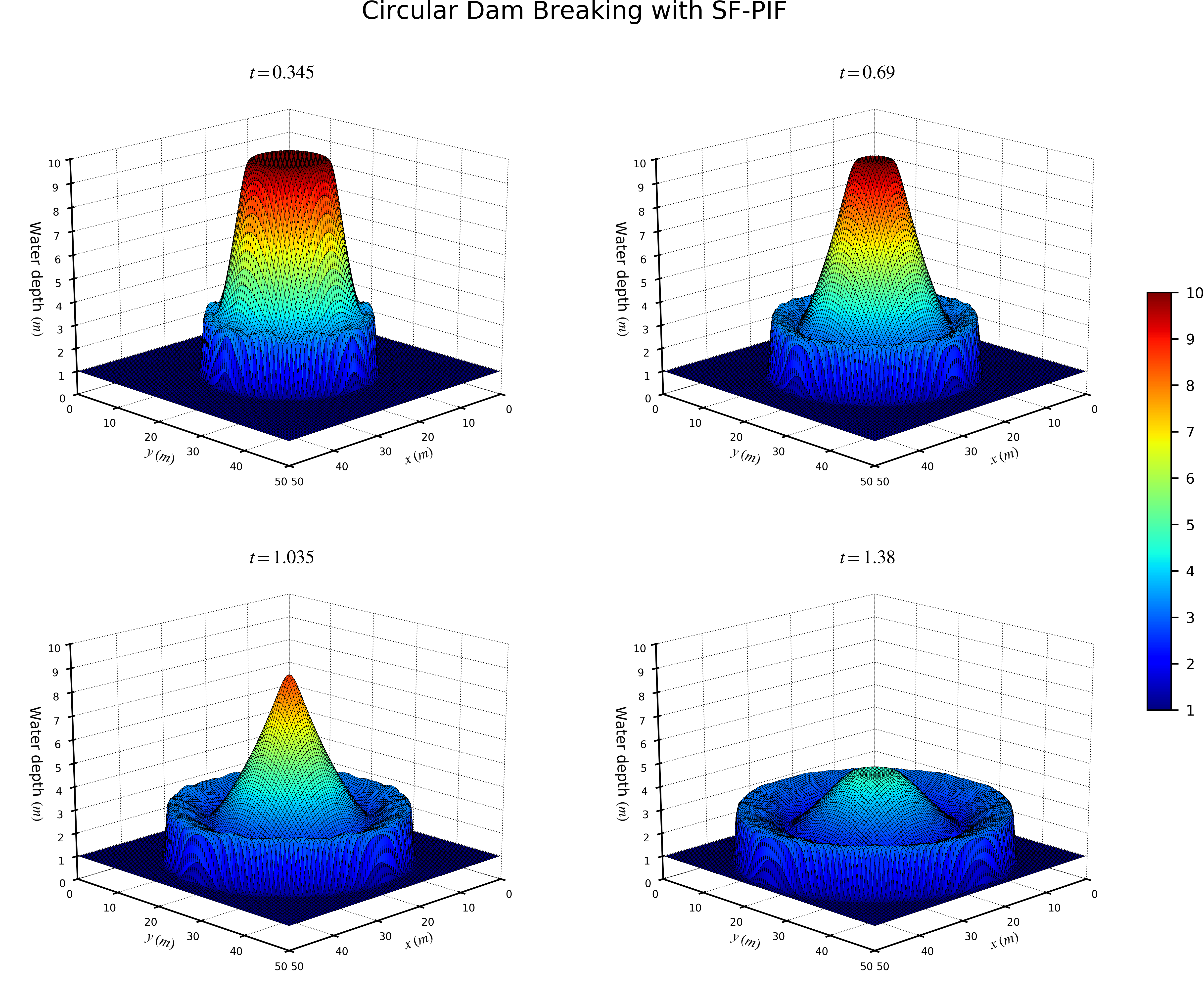
Figure 10: Snapshots of the circular dam breaking simulation at four different times, $t=0.345,0.69,1.035,$ and $1.38$ seconds. A volume of water in rest is initially confined in a cylindrical dam of a radius $r=11$ m and a height $h=10$ m. The simulation starts with an instantaneous removal of the cylindrical wall located at the center of the domain $\left[$50\text{\,}\mathrm{m}$\times$50\text{\,}\mathrm{m}$\right]$. The gravitational force is exerted on the steady water, which triggers the onset of the gravitational collapse of the entire volume of water, making the circular splash in the outer rim as well as the ripple effects in the central region that move radially outward in time.

As shown in Fig. 10, the results with SF-PIF are well comparable with the results using the same configuration reported in [68, 69, 70]. We conclude that the overall spherical symmetry and the sharp profile at the wave front are well maintained in the snapshots at four different times, $t=0.345,0.69,1.035$, and $1.38$.

5 Conclusion

In this paper, we have improved the flexibility of the PIF method in [40] by introducing a new Jacobian-free and Hessian-free approach. With this improvement, referred to as the system-free (SF) approach, the resulting SF-PIF method can be readily implemented in any existing RK-based FDM codes by swapping any multi-stage RK integrators with the single step, third-order accurate SF-PIF integrator.

The major advantage of SF-PIF lies in ease of its code implementation for practical use. In particular, SF-PIF can be applied easily to a different hyperbolic system of equations without hassle by virtue of our system-independent formulation of Jacobian-vector and Hessian-vector-vector multiplications, which operationally replaces the analytical expressions of the Jacobians and Hessians terms in the original PIF method.

In the present study, we have tested our SF-PIF algorithm to solve a wide range of well-known benchmark test problems in one and two spatial dimensions. The test results show that the solution accuracy and stability of SF-PIF are proved to be equally comparable with the solutions computed using arguably the most popular choice of the three-stage SSP-RK3 solver. Moreover, compared to RK3, SF-PIF achieves a twice fast code performance gain while maintaining the same third-order accuracy. We also have demonstrated that the SF-PIF method delivers the same order of accuracy as the original PIF method, while simplifying the calculations of the Jacobian and Hessian terms. The two methods are found to be nigh indistinguishable in their solution accuracy, stability, and performance. Mathematically speaking, the fact they are identical assures that the system-free approximation in SF-PIF is highly reliable in the Jacobian and Hessian term calculations in comparison with the analytical calculation in PIF. Practically speaking, as the SF-PIF method does not sensitively rely on a system of governing equations, it provides an increased adaptability to effortlessly switch to a different system of equations. This adaptability has been fully demonstrated in terms of switching the existing Euler equations code to a code for the shallow water equations in Section 4.3.

An extension of the current work is to design a fourth-order (or higher) SF-PIF method. However, a direct extension to a fourth-order scheme requires complex vector calculations and evaluations of the next high derivative terms, higher than the Hessian term in the Taylor expansion. Such a naive extension will be inevitably facing an increasing complexity in code implementations, and hence resulting the code performance less attractive in comparison with the use of conventional RK-based solvers. Reducing such complexities in designing a fourth- or higher-order SF-PIF method is essential, and a relevant work will be further investigated in our future studies.

6 Acknowledgements

We acknowledge use of the lux supercomputer at UC Santa Cruz, funded by NSF MRI grant AST 1828315. The authors thank Dr. Adam C. Reyes for very helpful discussions and feedback during the early stage of the development.

References

- [1] Norbert Attig, Paul Gibbon, and Th Lippert. Trends in supercomputing: The European path to exascale. Computer Physics Communications, 182(9):2041–2046, 2011.
- [2] ASCAC Subcommittee et al. Top ten exascale research challenges. US Department Of Energy Report, 2014.
- [3] Phillip Colella and Paul R Woodward. The piecewise parabolic method (PPM) for gas-dynamical simulations. Journal of computational physics, 54(1):174–201, 1984.
- [4] Guang-Shan Jiang and Chi-Wang Shu. Efficient implementation of weighted ENO schemes. Journal of computational physics, 126(1):202–228, 1996.
- [5] Sigal Gottlieb and Chi-Wang Shu. Total variation diminishing Runge-Kutta schemes. Mathematics of computation of the American Mathematical Society, 67(221):73–85, 1998.
- [6] Sigal Gottlieb, Chi-Wang Shu, and Eitan Tadmor. Strong stability-preserving high-order time discretization methods. SIAM review, 43(1):89–112, 2001.
- [7] Sigal Gottlieb, David I Ketcheson, and Chi-Wang Shu. Strong stability preserving Runge-Kutta and multistep time discretizations. World Scientific, 2011.
- [8] Dinshaw S Balsara and Chi-Wang Shu. Monotonicity preserving weighted essentially non-oscillatory schemes with increasingly high order of accuracy. Journal of Computational Physics, 160(2):405–452, 2000.
- [9] Andrea Mignone, Petros Tzeferacos, and Gianluigi Bodo. High-order conservative finite difference GLM–MHD schemes for cell-centered MHD. Journal of Computational Physics, 229(17):5896–5920, 2010.
- [10] Raymond J Spiteri and Steven J Ruuth. A new class of optimal high-order strong-stability-preserving time discretization methods. SIAM Journal on Numerical Analysis, 40(2):469–491, 2002.
- [11] Raymond J Spiteri and Steven J Ruuth. Non-linear evolution using optimal fourth-order strong-stability-preserving Runge-Kutta methods. Mathematics and Computers in Simulation, 62(1-2):125–135, 2003.
- [12] Steven J Ruuth and Raymond J Spiteri. Two barriers on strong-stability-preserving time discretization methods. Journal of Scientific Computing, 17(1-4):211–220, 2002.
- [13] Andrew Giuliani and Lilia Krivodonova. On the optimal CFL number of SSP methods for hyperbolic problems. Applied Numerical Mathematics, 135:165–172, 2019.
- [14] EF Toro, RC Millington, and LAM Nejad. Towards very high order Godunov schemes. In Godunov methods, pages 907–940. Springer, 2001.
- [15] Bram Van Leer. Towards the ultimate conservative difference scheme. v. a second-order sequel to Godunov’s method. Journal of computational Physics, 32(1):101–136, 1979.
- [16] Matania Ben-Artzi and Joseph Falcovitz. A second-order Godunov-type scheme for compressible fluid dynamics. Journal of Computational Physics, 55(1):1–32, 1984.
- [17] Matania Ben-Artzi and Jiequan Li. Hyperbolic balance laws: Riemann invariants and the generalized Riemann problem. Numerische Mathematik, 106(3):369–425, 2007.
- [18] Vladimir A Titarev and Eleuterio F Toro. ADER: Arbitrary high order Godunov approach. Journal of Scientific Computing, 17(1-4):609–618, 2002.
- [19] Vladimir A Titarev and Eleuterio F Toro. ADER schemes for three-dimensional non-linear hyperbolic systems. Journal of Computational Physics, 204(2):715–736, 2005.
- [20] Michael Dumbser, Dinshaw S Balsara, Eleuterio F Toro, and Claus-Dieter Munz. A unified framework for the construction of one-step finite volume and discontinuous Galerkin schemes on unstructured meshes. Journal of Computational Physics, 227(18):8209–8253, 2008.
- [21] Dinshaw S Balsara, Tobias Rumpf, Michael Dumbser, and Claus-Dieter Munz. Efficient, high accuracy ADER-WENO schemes for hydrodynamics and divergence-free magnetohydrodynamics. Journal of Computational Physics, 228(7):2480–2516, 2009.
- [22] Dinshaw S Balsara. Higher-order accurate space-time schemes for computational astrophysics—part I: finite volume methods. Living reviews in computational astrophysics, 3(1):2, 2017.
- [23] Dinshaw S Balsara, Chad Meyer, Michael Dumbser, Huijing Du, and Zhiliang Xu. Efficient implementation of ADER schemes for Euler and magnetohydrodynamical flows on structured meshes—speed comparisons with Runge-Kutta methods. Journal of Computational Physics, 235:934–969, 2013.
- [24] Michael Dumbser, Olindo Zanotti, Arturo Hidalgo, and Dinshaw S Balsara. ADER-WENO finite volume schemes with space–time adaptive mesh refinement. Journal of Computational Physics, 248:257–286, 2013.
- [25] Francesco Fambri, Michael Dumbser, and Olindo Zanotti. Space–time adaptive ADER-DG schemes for dissipative flows: Compressible Navier-Stokes and resistive MHD equations. Computer Physics Communications, 220:297–318, 2017.
- [26] Stéphane Clain, Steven Diot, and Raphaël Loubère. A high-order finite volume method for systems of conservation laws—multi-dimensional optimal order detection (MOOD). Journal of computational Physics, 230(10):4028–4050, 2011.
- [27] Steven Diot, Stéphane Clain, and Raphaël Loubère. Improved detection criteria for the multi-dimensional optimal order detection (MOOD) on unstructured meshes with very high-order polynomials. Computers & Fluids, 64:43–63, 2012.
- [28] Steven Diot, Raphaël Loubère, and Stephane Clain. The multidimensional optimal order detection method in the three-dimensional case: very high-order finite volume method for hyperbolic systems. International Journal for Numerical Methods in Fluids, 73(4):362–392, 2013.
- [29] Walter Boscheri, Raphaël Loubère, and Michael Dumbser. Direct arbitrary-lagrangian–Eulerian ADER-MOOD finite volume schemes for multidimensional hyperbolic conservation laws. Journal of Computational Physics, 292:56–87, 2015.
- [30] Raphaël Loubere, Michael Dumbser, and Steven Diot. A new family of high order unstructured MOOD and ADER finite volume schemes for multidimensional systems of hyperbolic conservation laws. Communications in Computational Physics, 16(3):718–763, 2014.
- [31] Olindo Zanotti and Michael Dumbser. Efficient conservative ADER schemes based on WENO reconstruction and space–time predictor in primitive variables. Computational astrophysics and cosmology, 3(1):1, 2016.
- [32] Matthew R Norman and Hal Finkel. Multi-moment ADER-Taylor methods for systems of conservation laws with source terms in one dimension. Journal of Computational Physics, 231(20):6622–6642, 2012.
- [33] Matthew R Norman. Algorithmic improvements for schemes using the ADER time discretization. Journal of Computational Physics, 243:176–178, 2013.
- [34] Matthew R Norman. A WENO-limited, ADER-DT, finite-volume scheme for efficient, robust, and communication-avoiding multi-dimensional transport. Journal of Computational Physics, 274:1–18, 2014.
- [35] L Del Zanna, O Zanotti, N Bucciantini, and P Londrillo. ECHO: a Eulerian conservative high-order scheme for general relativistic magnetohydrodynamics and magnetodynamics. Astronomy & Astrophysics, 473(1):11–30, 2007.
- [36] Yuxi Chen, Gábor Tóth, and Tamas I Gombosi. A fifth-order finite difference scheme for hyperbolic equations on block-adaptive curvilinear grids. Journal of Computational Physics, 305:604–621, 2016.
- [37] Adam Reyes, Dongwook Lee, Carlo Graziani, and Petros Tzeferacos. A variable high-order shock-capturing finite difference method with GP-WENO. Journal of Computational Physics, 381:189–217, 2019.
- [38] Ernst Hairer and Gerhard Wanner. Multistep-multistage-multiderivative methods for ordinary differential equations. Computing, 11(3):287–303, 1973.
- [39] David C Seal, Yaman Güçlü, and Andrew J Christlieb. High-order multiderivative time integrators for hyperbolic conservation laws. Journal of Scientific Computing, 60(1):101–140, 2014.
- [40] Andrew J Christlieb, Yaman Guclu, and David C Seal. The Picard integral formulation of weighted essentially nonoscillatory schemes. SIAM Journal on Numerical Analysis, 53(4):1833–1856, 2015.
- [41] David C Seal, Qi Tang, Zhengfu Xu, and Andrew J Christlieb. An explicit high-order single-stage single-step positivity-preserving finite difference WENO method for the compressible Euler equations. Journal of Scientific Computing, 68(1):171–190, 2016.
- [42] Jianxian Qiu and Chi-Wang Shu. Finite difference WENO schemes with Lax-Wendroff-type time discretizations. SIAM Journal on Scientific Computing, 24(6):2185–2198, 2003.
- [43] Yan Jiang, Chi-Wang Shu, and Mengping Zhang. An alternative formulation of finite difference weighted ENO schemes with Lax-Wendroff time discretization for conservation laws. SIAM Journal on Scientific Computing, 35(2):A1137–A1160, 2013.
- [44] Sergei Konstantinovich Godunov. A difference method for numerical calculation of discontinuous solutions of the equations of hydrodynamics. Matematicheskii Sbornik, 89(3):271–306, 1959.
- [45] Dongwook Lee, Hugues Faller, and Adam Reyes. The piecewise cubic method (PCM) for computational fluid dynamics. Journal of Computational Physics, 341:230–257, 2017.
- [46] Peter N Brown and Youcef Saad. Hybrid Krylov methods for nonlinear systems of equations. SIAM Journal on Scientific and Statistical Computing, 11(3):450–481, 1990.
- [47] Dana A Knoll and David E Keyes. Jacobian-free Newton-Krylov methods: a survey of approaches and applications. Journal of Computational Physics, 193(2):357–397, 2004.
- [48] Dana A Knoll, H Park, and Kord Smith. Application of the Jacobian-free Newton-Krylov method to nonlinear acceleration of transport source iteration in slab geometry. Nuclear Science and Engineering, 167(2):122–132, 2011.
- [49] Charles William Gear and Youcef Saad. Iterative solution of linear equations in ODE codes. SIAM journal on scientific and statistical computing, 4(4):583–601, 1983.
- [50] Heng-Bin An, Ju Wen, and Tao Feng. On finite difference approximation of a matrix-vector product in the Jacobian-free Newton-Krylov method. Journal of Computational and Applied Mathematics, 236(6):1399–1409, 2011.
- [51] James Kent, Jared P Whitehead, Christiane Jablonowski, and Richard B Rood. Determining the effective resolution of advection schemes. part I: Dispersion analysis. Journal of Computational Physics, 278:485–496, 2014.
- [52] James Kent, Christiane Jablonowski, Jared P Whitehead, and Richard B Rood. Determining the effective resolution of advection schemes. part II: Numerical testing. Journal of Computational Physics, 278:497–508, 2014.
- [53] Gary A Sod. A survey of several finite difference methods for systems of nonlinear hyperbolic conservation laws. Journal of computational physics, 27(1):1–31, 1978.
- [54] Paul Woodward and Phillip Colella. The numerical simulation of two-dimensional fluid flow with strong shocks. Journal of computational physics, 54(1):115–173, 1984.
- [55] Chi-Wang Shu and Stanley Osher. Efficient implementation of essentially non-oscillatory shock-capturing schemes, II. In Upwind and High-Resolution Schemes, pages 328–374. Springer, 1989.
- [56] Chi-Wang Shu. Essentially non-oscillatory and weighted essentially non-oscillatory schemes for hyperbolic conservation laws. In Advanced numerical approximation of nonlinear hyperbolic equations, pages 325–432. Springer, 1998.
- [57] Seth C Spiegel, HT Huynh, and James R DeBonis. A survey of the isentropic Euler vortex problem using high-order methods. In 22nd AIAA Computational Fluid Dynamics Conference, page 2444, 2015.
- [58] Tong Zhang and Yu Xi Zheng. Conjecture on the structure of solutions of the Riemann problem for two-dimensional gas dynamics systems. SIAM Journal on Mathematical Analysis, 21(3):593–630, 1990.
- [59] Carsten W Schulz-Rinne. Classification of the Riemann problem for two-dimensional gas dynamics. SIAM journal on mathematical analysis, 24(1):76–88, 1993.
- [60] Carsten W Schulz-Rinne, James P Collins, and Harland M Glaz. Numerical solution of the Riemann problem for two-dimensional gas dynamics. SIAM Journal on Scientific Computing, 14(6):1394–1414, 1993.
- [61] Dinshaw S Balsara. Multidimensional HLLE Riemann solver: Application to Euler and magnetohydrodynamic flows. Journal of Computational Physics, 229(6):1970–1993, 2010.
- [62] Pawel Buchmüller and Christiane Helzel. Improved accuracy of high-order WENO finite volume methods on Cartesian grids. Journal of Scientific Computing, 61(2):343–368, 2014.
- [63] Wai-Sun Don, Zhen Gao, Peng Li, and Xiao Wen. Hybrid compact-WENO finite difference scheme with conjugate Fourier shock detection algorithm for hyperbolic conservation laws. SIAM Journal on Scientific Computing, 38(2):A691–A711, 2016.
- [64] WH Hui, PY Li, and ZW Li. A unified coordinate system for solving the two-dimensional Euler equations. Journal of Computational Physics, 153(2):596–637, 1999.
- [65] Richard Liska and Burton Wendroff. Comparison of several difference schemes on 1D and 2D test problems for the Euler equations. SIAM Journal on Scientific Computing, 25(3):995–1017, 2003.
- [66] James M Stone, Thomas A Gardiner, Peter Teuben, John F Hawley, and Jacob B Simon. Athena: a new code for astrophysical MHD. The Astrophysical Journal Supplement Series, 178(1):137, 2008.
- [67] Friedemann Kemm. On the proper setup of the double Mach reflection as a test case for the resolution of gas dynamics codes. Computers & Fluids, 132:72–75, 2016.
- [68] Francisco Alcrudo and Pilar Garcia-Navarro. A high-resolution Godunov-type scheme in finite volumes for the 2D shallow-water equations. International Journal for Numerical Methods in Fluids, 16(6):489–505, 1993.
- [69] Eleuterio F Toro. Shock-capturing methods for free-surface shallow flows. John Wiley, 2001.
- [70] Anargiros I Delis and Th Katsaounis. Numerical solution of the two-dimensional shallow water equations by the application of relaxation methods. Applied Mathematical Modelling, 29(8):754–783, 2005.