Flow and structure in nonequilibrium Brownian many-body systems

Abstract

We present a fundamental classification of forces relevant in nonequilibrium structure formation under collective flow in Brownian many-body systems. The internal one-body force field is systematically split into contributions relevant for the spatial structure and for the coupled motion. We demonstrate that both contributions can be obtained straightforwardly in computer simulations, and present a power functional theory that describes all types of forces quantitatively. Our conclusions and methods are relevant for flow in inertial systems, such as molecular liquids and granular media.

Nonequilibrium phenomenology in colloidal systems is both diverse and poorly understood. Examples include lane Dzubiella et al. (2002) and band Vissers et al. (2011) formation in oppositely driven colloids, the motility induced phase separation in active systems Cates and Tailleur (2015); Digregorio et al. (2018), the migration of colloidal particles induced by shear fields Lyon and Leal (1998); Frank et al. (2003a), and magnetically controlled dynamical self-assembly Snezhko and Aranson (2011). Even the universal processes of vitrification Golde et al. (2016) and crystallization Tan et al. (2014) are still not well understood.

Our inability to properly describe nonequilibrium phenomena can be traced back to our lack of understanding of the internal force field, that is, the one-body field that originates from a position- and time-resolved average of the interparticle interactions. In equilibrium, the internal force field depends only on the density distribution and it is well described by the widely used framework of density functional theory (DFT) Evans (1979). In contrast, in non-equilibrium, the internal force field depends on both the density and the flow Schmidt and Brader (2013); de las Heras et al. (2019). We show here that the nonequilibrium internal force field naturally splits into four fundamentally different contributions and we provide a method to measure each of them using computer simulations. The classification of the internal forces is based on the direction of the force and, crucially, on whether the force acts on the particle flow or on the structure of the fluid. We show how flow and spatial structure, which are often treated separately, naturally interplay in generating the internal force field and, therefore, provide a unifying framework to treat both aspects on equal footing. Finally, we present a microscopic theory, based on the power functional Schmidt and Brader (2013), that predicts quantitatively all occurring types of contributions to the internal force field across a range of fundamentally different nonequilibrium situations.

Consider a nonequilibrium overdamped Brownian system with no hydrodynamic interactions. The time evolution is given by the exact one-body equation of motion

$$\gamma{\bf v}({\mathbf{r}},t) ={\bf f}_{\rm tot}({\mathbf{r}},t),$$ (1)

and the continuity equation

$$\frac{\partial}{\partial t}\rho({\mathbf{r}},t)=-\nabla\cdot{\bf J}({\mathbf{r}},t),$$ (2)

where $\gamma$ is the single-particle friction constant against the (implicit) solvent, ${\bf v}({\mathbf{r}},t)$ is the velocity field at position ${\mathbf{r}}$ and time $t$, ${\bf f}_{\rm tot}({\mathbf{r}},t)$ is the total force field, $\rho({\mathbf{r}},t)$ is the density distribution, and ${\bf J}=\rho{\bf v}$ is the current profile. The total force comprises three contributions,

$${\bf f}_{\rm tot} ={\bf f}_{\rm ext}+{\bf f}_{\rm int}+{\bf f}_{\rm id},$$ (3)

with the imposed external force field ${\bf f}_{\rm ext}$, the internal force field ${\bf f}_{\rm int}$, and the ideal-gas diffusion ${\bf f}_{\rm id}=-k_{B}T\nabla\ln\rho$; here $k_{B}$ is the Boltzmann constant and $T$ is absolute temperature. All one-body fields above are well-defined as statistical averages of microscopic operators, see e.g. de las Heras et al. (2019). The underlying many-body dynamics are given, equivalently, by a Fokker-Planck (Smoluchowski) equation for the probability distribution or in the Langevin picture of stochastic trajectories.

The internal force consists of adiabatic and superadiabatic contributions ${\bf f}_{\rm int}={\bf f}_{\rm ad}+{\bf f}_{\rm sup}$ Schmidt and Brader (2013); Fortini et al. (2014). The equilibrium-like adiabatic part, ${\bf f}_{\rm ad}$, is the only internal force that enters in the widespread dynamical density functional theory Marconi and Tarazona (1999) and it describes the internal forces in a hypothetical equilibrium system (vanishing current) with the same density distribution as the actual nonequilibrium system. In contrast, the superadiabatic force field, ${\bf f}_{\rm sup}$, is of purely out-of-equilibrium origin. Both ${\bf f}_{\rm ad}$ and ${\bf f}_{\rm sup}$ can be written as functional derivatives using DFT Evans (1979) and power functional theory (PFT) Schmidt and Brader (2013), respectively.

Although the continuity equation (2) links the flow ${\bf v}$ and the density profile $\rho$, there is much freedom in choosing both fields separately. PFT assures that a mapping from $\rho$ and ${\bf v}$ to the external force exists Schmidt and Brader (2013); de las Heras et al. (2019). Hence $\rho$ and ${\bf v}$ constitute genuine variables rather than being the result of a prescribed driving mechanism. It is possible to find e.g. two systems that share the same density profile, but have different velocity profiles. A simple situation consists of a family of flows differing only in magnitude of the velocity de las Heras et al. (2019). However, much more complex cases exist, since the continuity equation (2) does not impose any restriction on the curl of the current. Hence the addition of any divergence–free vector field to the current keeps the continuity equation satisfied with identical density profile. There exist also systems that share the same flow but posses different density profiles. It is therefore natural to split the equation of motion (1) into two interrelated equations, one for the flow and one for the structure, given respectively by

$$\gamma{\bf v} ={\bf f}_{\rm flow}+{\bf f}_{\rm ext,f},$$ (4)

$$0 ={\bf f}_{\rm id}+{\bf f}_{\rm ad}+{\bf f}_{\rm str}+{\bf f}_{\rm ext,s}.$$ (5)

The diffusive term, ${\bf f}_{\rm id}$, and the adiabatic force, ${\bf f}_{\rm ad}$, depend only on the density profile, and therefore act on the structure (5). The external force can act on both structure and flow and therefore it splits into a contribution that acts on the flow, ${\bf f}_{\rm ext,f}$, and one that acts on the structure, ${\bf f}_{\rm ext,s}$, such that ${\bf f}_{\rm ext}={\bf f}_{\rm ext,f}+{\bf f}_{\rm ext,s}$. The total superadiabatic force field, ${\bf f}_{\rm sup}$, also acts on both flow and structure and hence can be split according to

$${\bf f}_{\rm sup}={\bf f}_{\rm flow}+{\bf f}_{\rm str}.$$ (6)

Equations (4) and (5) are coupled since ${\bf f}_{\rm flow}$ and ${\bf f}_{\rm str}$ are functionals of both $\rho$ and ${\bf v}$. However, both equations describe different phenomena; the velocity field is determined by the flow, Eq. (4), whereas the density profile is given by the structural force balance (5). As we demonstrate below, both superadiabatic forces behave differently under motion reversal.

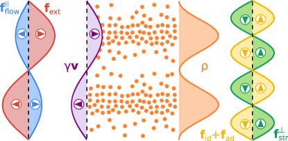
Figure 1: Force balance in Kolmogorov flow. A colloidal system is driven with a sinusoidal external force ${\bf f}_{\rm ext}$ (red). The force creates a flow $\gamma{\bf v}$ (violet) that generates a superadiabatic flow force ${\bf f}_{\rm flow}^{||}$ (blue) of viscous nature and a density modulation $\rho$ (orange) which is the result of the force balance between the superadiabatic structural, ${\bf f}_{\rm str}^{\perp}$ (green) and the sum of adiabatic ${\bf f}_{\rm ad}$ and diffusive ${\bf f}_{\rm id}$ (yellow) forces. The arrows indicate the directions of the forces. An illustrative microstate is shown with particles depicted as orange circles.

To gain insight into the physical properties of (6), we address first the force balance of the well-known phenomenon of shear migration Leighton and Acrivos (1987); Frank et al. (2003b). A broad range of further types of drivings are analysed below. For simplicity we consider steady states, where all one-body quantities are time independent and hence $\nabla\cdot{\bf J}=0$, cf. (2).

Consider a colloidal system undergoing a Kolmogorov-like flow Obukhov (1983), see Fig. 1. The particles are driven by a sinusoidal external field ${\bf f}_{\rm ext}\propto\sin(y)\hat{\mathbf{x}}$ (red) which creates a steady state with a flow ${\bf v}$ parallel to the driving (violet) in ${x}$-direction. In the direction perpendicular to the flow, a density modulation $\rho({\mathbf{r}})=\rho(y)$ (orange) appears since the particles migrate towards the region of low shear rate. The superadiabatic forces here are easy to interpret Stuhlmüller et al. (2018). A dissipative viscous-like force ${\bf f}_{\rm flow}^{||}$ (blue) opposes the flow. The force is anti-parallel to the flow and it clearly changes direction if the external driving is reversed. The density modulation in the direction perpendicular to the flow is sustained by a nondissipative structural superadiabatic force ${\bf f}_{\rm str}^{\perp}$ (green) that remains unchanged under flow reversal and that cancels both the diffusive and the adiabatic forces (yellow). In this geometry, the flow forces are of viscous nature and parallel to the flow, whereas the structural forces are perpendicular to it. As both superadiabatic components are orthogonal to each other, measuring them separately in computer simulations is simple. However, in general we expect also structural forces to occur parallel to the flow, ${\bf f}_{\rm str}^{||}$, and flow forces to occur perpendicular to the flow, ${\bf f}_{\rm flow}^{\perp}$. To split the superadiabatic forces into all these constituents, we consider what we call “reverse” or ”backward” state, which possess the same density profile as the original “forward” state but it has the opposite flow. Hence, indicating quantities in the reverse state by a prime, we have

$$\rho^{\prime}({\mathbf{r}})=\rho({\mathbf{r}}),\quad{\bf v}^{\prime}({\mathbf{r}})=-{\bf v}({\mathbf{r}}).$$ (7)

As a direct consequence of the structure of  (4) and (5), the flow component of the superadiabatic force reverses it sign in the reverse state (${\bf f}_{\rm flow}^{\prime}=-{\bf f}_{\rm flow}$), whereas the structural component remains unchanged (${\bf f}_{\rm str}^{\prime}={\bf f}_{\rm str}$), i.e.,

$${\bf f}_{\rm sup}^{\prime}={\bf f}_{\rm flow}^{\prime}+{\bf f}_{\rm str}^{\prime}=-{\bf f}_{\rm flow}+{\bf f}_{\rm str}.$$ (8)

Once flow and structural components have been identified, we project the vector fields onto the directions parallel $(||)$ and perpendicular $(\perp)$ to the velocity field. The final and complete splitting of superadiabatic forces is

$${\bf f}_{\rm sup}={\bf f}_{\rm flow}^{||}+{\bf f}_{\rm flow}^{\perp}+{\bf f}_{\rm str}^{||}+{\bf f}_{\rm str}^{\perp}.$$ (9)

The ideal diffusion and the adiabatic forces do not change in the reverse state since they only depend on the density profile, i.e., ${\bf f}_{\rm id}^{\prime}={\bf f}_{{\rm id}}$ and ${\bf f}_{\rm ad}^{\prime}={\bf f}_{{\rm ad}}$. Therefore, using  (1) and (8), we arrive at the following equations of motion in the forward and in the reverse states, respectively,

$$\gamma{\bf v} ={\bf f}_{{\rm id}}+{\bf f}_{{\rm ad}}+{\bf f}_{{\rm flow}}+{\bf f}_{{\rm str}}+{\bf f}_{{\rm ext}},$$ (10)

$$-\gamma{\bf v} ={\bf f}_{{\rm id}}+{\bf f}_{{\rm ad}}-{\bf f}_{{\rm flow}}+{\bf f}_{{\rm str}}+{\bf f}_{\rm ext}^{\prime}.$$ (11)

Adding and subtracting (10) and (11) yields:

$${\bf f}_{{\rm flow}} = \gamma{\bf v}-\left({\bf f}_{{\rm ext}}-{\bf f}_{\rm ext}^{\prime}\right)/2,$$ (12)

$${\bf f}_{{\rm str}} = -{\bf f}_{{\rm id}}-{\bf f}_{{\rm ad}}-\left({\bf f}_{{\rm ext}}+{\bf f}_{\rm ext}^{\prime}\right)/2.$$ (13)

Alternatively, from (6) and (8) it follows that

$${\bf f}_{\rm flow} =\left({\bf f}_{\rm sup}-{\bf f}_{\rm sup}^{\prime}\right)/2,$$ (14)

$${\bf f}_{\rm str} =\left({\bf f}_{\rm sup}+{\bf f}_{\rm sup}^{\prime}\right)/2.$$ (15)

The final steps to apply either Eqs. (12)-(13) or (14)-(15) are (i) to find the external force ${\bf f}^{\prime}_{\rm ext}$ that reverses the flow and (ii) to split the internal force field, ${\bf f}_{\rm int}$, into adiabatic and superadiabatic contributions. In general ${\bf f}_{\rm ext}^{\prime}\neq-{\bf f}_{\rm ext}$ due to nonvanishing structural (flow) forces (parallel) perpendicular to the flow, see Eqs. (10)-(11).

The four components of the superadiabatic forces (9) are accessible in many-body BD simulations. In Ref. de las Heras et al. (2019) we developed an iterative method to construct the external force field that generates a given (prescribed) time evolution of a Brownian system; a brief description is provided in the Supplemental Material (SM) Sup . Using this “custom flow” method it is straightforward to calculate in BD simulations ${\bf f}_{{\rm ext}}^{\prime}$ since $\rho$ and ${\bf v}$ are known, see Eq. (7). Splitting the internal force field into adiabatic and superadiabatic contributions is also simple Fortini et al. (2014); de las Heras et al. (2019): we first find the adiabatic external force ${\bf f}_{\rm ext}^{\rm ad}$, i.e. the conservative external force field that generates the desired density profile in equilibrium (${\bf v}=0$). To this end we use the method of Ref. de las Heras et al. (2019). The adiabatic force ${\bf f}_{\rm ad}$ is then the internal force in presence of ${\bf f}_{\rm ext}^{\rm ad}$. The superadiabatic force is the difference between the total internal and the adiabatic fields, ${\bf f}_{\rm sup}={\bf f}_{\rm int}-{\bf f}_{\rm ad}$.

Knowledge of the superadiabatic forces in the forward and in the reverse states gives direct access to the flow and the structural components via (14) and (15). Using ${\bf f}_{\rm ext}^{\rm ad}$ the structural force (13) can be also expressed using only external forces ${\bf f}_{\rm str}={\bf f}_{\rm ext}^{\rm ad}-({\bf f}_{{\rm ext}}+{\bf f}_{\rm ext}^{\prime})/2$ since in the adiabatic (equilibrium) system ${\bf f}_{\rm ext}^{\rm ad}+{\bf f}_{\rm id}+{\bf f}_{\rm ad}=0$. Once the flow and the structural components are known, we project them onto the local flow direction, given by $\hat{\mathbf{e}}_{v}({\mathbf{r}})={\bf v}({\mathbf{r}})/|{\bf v}({\mathbf{r}})|$, to obtain the parallel and perpendicular components,

$${\bf f}_{\alpha}^{||}=({\bf f}_{\alpha}\cdot\hat{\mathbf{e}}_{v})\hat{\mathbf{e}}_{v},\quad{\bf f}_{\alpha}^{\perp}={\bf f}_{\alpha}-{\bf f}_{\alpha}^{||},\quad\alpha=\{\rm flow,\rm str\}.$$ (16)

We study the fundamental splitting (9) of the superadiabatic forces in a simple two-dimensional system of purely repulsive particles (Weeks-Chandler-Anderson potential Weeks et al. (1971) with $\sigma$ and $\epsilon$ as length and energy parameters, respectively). The particles are confined in a square box of length $h$ (centered at the origin) with periodic boundary conditions, see Fig. 2a.

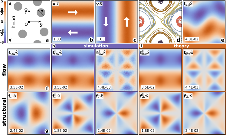
Figure 2: Superadiabatic forces. (a) Schematic of the simulation box. Sampled (b) ${x}$- and (c) ${y}$-components of the imposed steady state velocity profile. (d) Characteristic trajectories followed by the particles in absence of Brownian noise. (e) ${x}$-component of the total superadiabatic force measured in BD. Flow (f) and structural (g) components of the superadiabatic force according to BD. (h) Splitting of flow and structural forces into their parallel and perpendicular components, as indicated. Data obtained with BD simulations. (i) Same as (h) but using power functional theory. All forces are in units of $\epsilon/\sigma$. The flow is in units of $\tau/\sigma$. The scale factor $s$ (see color bar) is indicated in each plot. The $y$-components are depicted in the SM Sup .

To illustrate the classification of the superadiabatic forces, we analyse eight different steady states. We use custom flow de las Heras et al. (2019); Sup to impose ${\bf v}$ and $\rho$ and then find the corresponding external fields both in the forward and in the reverse states. The steady states cover fundamentally different cases such as divergence-free flow, curl-free flow, and families of flows with the same velocity profiles but different density profiles. The description of the flows along with plots of all forces and simulation details are given in the SM Sup . Here, we just illustrate the complexity and richness of the superadiabatic forces for a representative example (flow number $1$ in SM Sup ). The imposed steady state is a generalized Kolmogorov flow, in which each component of the velocity is a pure sinusoidal wave,

$${\bf v}({\mathbf{r}})=\left(\begin{matrix}v_{0}\sin(2\pi y/h)\\ v_{0}\sin(2\pi x/h)\end{matrix}\right),\;\;\rho({\mathbf{r}})=\rho_{0},$$ (17)

with $v_{0}\tau/\sigma=1.0$, constant density $\rho_{0}=0.2\sigma^{-2}$, and $\tau=\sigma^{2}\gamma/\epsilon$ is the time unit. The two Cartesian velocity components sampled in BD simulations are shown in Fig. 2b and 2c. Illustrative particle trajectories are shown in Fig. 2d: the particles wind around specific points, which constitute defects in the velocity field, i.e., points at which the direction of the velocity is ill-defined. To better highlight the motion, the trajectories were calculated in absence of Brownian motion. The imposed density profile is uniform, and therefore the ideal diffusive and the adiabatic force fields, both gradient fields, vanish identically. The internal force field is hence purely superadiabatic. In Fig. 2e we show the ${x}$-component of the superadiabatic force field. Due to the symmetry of the flow, the ${y}$-component (shown in SM Sup ) is simply the ${x}$-component after a ninety degrees anticlockwise rotation about the origin followed by a reflection through the ${y}$-axis. The splitting into flow and structural forces (6) is shown in Figs. 2f and 2g, respectively. Both force fields are of the same order of magnitude but they play different roles. The flow force is mostly of viscous nature opposing the direction of motion. The structural force is dominated by a migration-like term. It is quite complex, as it tends to move the particles towards the defects with cyclonic vorticity (those located at the middle of the sides of the box), away from the hyperbolic defects (center and corners of the box). The density is, however, constant by construction and therefore the structural force does not create any density modulation. Instead, the structural force is balanced by the structural component of the external field, ${\bf f}_{\rm ext,s}$, cf. (5). The external force field performs two different tasks: (i) it creates the flow and (ii) it compensates the structural forces that are generated as a result of the flow.

The full splitting into the four types of nonequilibrium forces (9) is shown in Fig. 2h. Clearly all types of forces, including the flow forces perpendicular to the flow and the structural forces parallel to the flow exist, and no contribution is negligible. The parallel flow force ${\bf f}_{\rm flow}^{||}$ can be understood as arising from viscosity. However, although the flow is made of pure sinusoidal waves, ${\bf f}_{\rm flow}^{||}$ exhibits a complex spatial structure and it is not a simple sine wave opposing the flow, as one would naively expect according to a Navier-Stokes description of the viscous force. Moreover, the perpendicular component of the flow force is highly non-trivial and cannot be interpreted as a viscous response.

Although this example is restricted to a case of homogeneous density, we show in the SM Sup a variety of steady states with inhomogeneous density profiles. The versatility of the custom flow method allows us to e.g. analyse a steady state (flow number $2$) with the same velocity profile as in (17) but with an inhomogeneous density profile. Comparing systems with the same ${\bf v}$ but different $\rho$ is useful to gain insight into the structure of the power functional that generates the superadiabatic forces.

The superadiabatic forces are functional derivatives of the functional $P_{t}^{\rm exc}$ with respect to the current Schmidt and Brader (2013); Sup . The splitting into flow and structural forces can be analyzed via a power series of the velocity field de las Heras and Schmidt (2018); Stuhlmüller et al. (2018). Terms odd (even) in powers of ${\bf v}$ lead to structural (flow) forces that must be even (odd) in powers of ${\bf v}$. Note that (i) the functional differentiation reduces by one the power of the velocity field, and (ii) flow (structural) forces change (do not change) sign upon flow reversal. The simplest approximation for $P_{t}^{\rm exc}$ is, in essence, a space integral of a quadratic form in the local velocity gradient de las Heras and Schmidt (2018). The resulting superadiabatic force is a flow force (no structural terms) that represent the viscous and shear responses in the Navier-Stokes equations. Higher order terms, third order in powers of the velocity field, are required to generate all the structural forces. These terms are based on spatial integrals of rotational invariants of the type ${\sf L}_{ijkl}(\nabla_{i}{\bf v}_{j})({\bf v}_{k})({\bf v}_{l})$ and ${\sf Q}_{ijklmn}(\nabla_{i}{\bf v}_{j})(\nabla_{k}{\bf v}_{l})(\nabla_{m}{\bf v}_{j})$ with ${\sf L}$ and ${\sf Q}$ isotropic tensors of rank fourth and sixth, respectively. We find it necessary to include fourth order terms to correctly describe the flow forces in some of the steady states analysed. The theory reproduces from first principles the complex shape of the superadiabatic forces computed in BD simulations (only the magnitude of the forces needs to be adjusted) Compare e.g. Figs. 2h (simulation) and 2i (PFT). Further comparisons and details about $P_{t}^{\rm exc}$ are provided in SM Sup .

Although we used custom flow de las Heras et al. (2019) to prescribe the flow, the splitting of superadiabatic forces is general and applies to the standard situation where ${\bf f}_{\rm ext}$ is prescribed instead of the flow itself. Custom flow is then required only to obtain the reverse state. The custom flow method also works in time-dependent nonequilibrium situations de las Heras et al. (2019). Hence the splitting of the superadiabatic forces can be done in any situation. Our analysis is devoted to overdamped Brownian systems without hydrodynamic interactions. Therefore, the superadiabatic forces are solely generated by the interparticle interactions in nonequilibrium. Using an inert solvent has allowed us to isolate the superadiabatic effects from those due to hydrodynamics. Inclusion of hydrodynamic effects can be effectively done via transport coefficients Sup in a modified form. For example, it has been shown recently that complex hydrodynamic effects, such as diffusion in complex liquids, can be correctly accounted for with wave vector dependent viscosities Makuch et al. (2020).

We expect the same type of superadiabatic forces to be present in other dynamical systems, including granular systems and inertial Newtonian dynamics such as e.g. molecular liquids. Within the Navier-Stokes equations one assumes (i) the viscous term to be proportional to the velocity gradient and (ii) omits the structural terms. Our results indicate both assumptions might not be acceptable even in very simple flows. We anticipate, e.g. that the structural forces play a crucial role in most nonequilibrium situations, including e.g., turbulent flows Iyer et al. (2019), crystallization Tan et al. (2014); Golde et al. (2016), and the hysteresis of the liquid-solid transition in granular systems Perrin et al. (2019).

References

- Dzubiella et al. (2002) J. Dzubiella, G. P. Hoffmann, and H. Löwen, “Lane formation in colloidal mixtures driven by an external field,” Phys. Rev. E 65, 021402 (2002).
- Vissers et al. (2011) T. Vissers, A. van Blaaderen, and A. Imhof, “Band formation in mixtures of oppositely charged colloids driven by an ac electric field,” Phys. Rev. Lett. 106, 228303 (2011).
- Cates and Tailleur (2015) M. E. Cates and J. Tailleur, “Motility-induced phase separation,” Annu. Rev. Condens. 6, 219 (2015).
- Digregorio et al. (2018) P. Digregorio, D. Levis, A. Suma, L. F. Cugliandolo, G. Gonnella, and I. Pagonabarraga, “Full phase diagram of active Brownian disks: From melting to motility-induced phase separation,” Phys. Rev. Lett. 121, 098003 (2018).
- Lyon and Leal (1998) M. K. Lyon and L. G. Leal, “An experimental study of the motion of concentrated suspensions in two-dimensional channel flow. part 1. monodisperse systems,” J. Fluid Mech. 363, 25 (1998).
- Frank et al. (2003a) M. Frank, D. Anderson, E. R. Weeks, and J. F. Morris, “Particle migration in pressure-driven flow of a Brownian suspension,” J. Fluid Mech. 493, 363 (2003a).
- Snezhko and Aranson (2011) A. Snezhko and I. S. Aranson, “Magnetic manipulation of self-assembled colloidal asters,” Nat. Mater. 10, 698 (2011).
- Golde et al. (2016) S. Golde, T. Palberg, and H. J. Schöpe, “Correlation between dynamical and structural heterogeneities in colloidal hard-sphere suspensions,” Nat. Phys. 12, 712 (2016).
- Tan et al. (2014) P. Tan, N. Xu, and L. Xu, “Visualizing kinetic pathways of homogeneous nucleation in colloidal crystallization,” Nat. Phys. 10, 73 (2014).
- Evans (1979) R. Evans, “The nature of the liquid-vapour interface and other topics in the statistical mechanics of non-uniform, classical fluids,” Adv. Phys. 28, 143 (1979).
- Schmidt and Brader (2013) M. Schmidt and J. M. Brader, “Power functional theory for Brownian dynamics,” J. Chem. Phys. 138 (2013).
- de las Heras et al. (2019) D. de las Heras, J. Renner, and M. Schmidt, “Custom flow in overdamped Brownian dynamics,” Phys. Rev. E 99, 023306 (2019).
- Fortini et al. (2014) A. Fortini, D. de las Heras, J. M. Brader, and M. Schmidt, “Superadiabatic forces in Brownian many-body dynamics,” Phys. Rev. Lett. 113, 167801 (2014).
- Marconi and Tarazona (1999) U. M. B. Marconi and P. Tarazona, “Dynamic density functional theory of fluids,” J. Chem. Phys. 110, 8032 (1999).
- Leighton and Acrivos (1987) D. Leighton and A. Acrivos, “The shear-induced migration of particles in concentrated suspensions,” J. Fluid Mech. 181, 415–439 (1987).
- Frank et al. (2003b) M. Frank, D. Anderson, E. R. Weeks, and J. F. Morris, “Particle migration in pressure-driven flow of a brownian suspension,” J. Fluid Mech. 493, 363–378 (2003b).
- Obukhov (1983) A. M. Obukhov, “Kolmogorov flow and laboratory simulation of it,” Russ. Math. Surv. 38, 113 (1983).
- Stuhlmüller et al. (2018) N. C. X. Stuhlmüller, T. Eckert, D. de las Heras, and M. Schmidt, “Structural nonequilibrium forces in driven colloidal systems,” Phys. Rev. Lett. 121, 098002 (2018).
- Weeks et al. (1971) J. D. Weeks, D. Chandler, and H. C. Andersen, “Role of repulsive forces in determining the equilibrium structure of simple liquids,” J. Chem. Phys. 54, 5237 (1971).
- (20) See supplemental material for details about simulations, theory, and several types of flows: www.danieldelasheras.com/docs/52-sm.pdf .
- de las Heras and Schmidt (2018) D. de las Heras and M. Schmidt, “Velocity gradient power functional for Brownian dynamics,” Phys. Rev. Lett. 120, 028001 (2018).
- Makuch et al. (2020) K. Makuch, R. Holyst, T. Kalwarczyk, P. Garstecki, and J. F. Brady, “Diffusion and flow in complex liquids,” Soft Matter 16, 114 (2020).
- Iyer et al. (2019) Kartik P. Iyer, Katepalli R. Sreenivasan, and P. K. Yeung, “Circulation in high reynolds number isotropic turbulence is a bifractal,” Phys. Rev. X 9, 041006 (2019).
- Perrin et al. (2019) H. Perrin, C. Clavaud, M. Wyart, B. Metzger, and Y. Forterre, “Interparticle friction leads to nonmonotonic flow curves and hysteresis in viscous suspensions,” Phys. Rev. X 9, 031027 (2019).