Quasi-orthonormal Encoding for Machine Learning Applications

Abstract

Most machine learning models, especially artificial neural networks, require numerical, not categorical data. We briefly describe the advantages and disadvantages of common encoding schemes. For example, one-hot encoding is commonly used for attributes with a few unrelated categories and word embeddings for attributes with many related categories (e.g., words). Neither is suitable for encoding attributes with many unrelated categories, such as diagnosis codes in healthcare applications. Application of one-hot encoding for diagnosis codes, for example, can result in extremely high dimensionality with low sample size problems or artificially induce machine learning artifacts, not to mention the explosion of computing resources needed. Quasi-orthonormal encoding (QOE) fills the gap. We briefly show how QOE compares to one-hot encoding. We provide example code of how to implement QOE using popular ML libraries such as Tensorflow and PyTorch and a demonstration of QOE to MNIST handwriting samples.

Keywords machine learning, classification, categorical encoding

machine learning, classification, categorical encoding

Introduction

While most popular machine learning methods such as deep learning require numerical data as input, categorical data is very common practice. For example, a person’s vitals could be a combination of both, they could include height, weight (numerical) and gender, race (categorical). The challenge is to convert the categorical data into a vector of some sort.

One-hot encoding which is discussed in the next section is very commonly used these days in machine learning but has the draw back that it can increase the dimensionality of the data by the cardinality of the category. For small category, this is not a significant issue but when categories with high cardinality are present, many problems can arise as described below.

Quasiorthonormal encoding (QOE) is a generalization of the one-hot encoding and exploits the fact that in high dimensional vector spaces, two random vectors are almost always orthogonal. The concept originated with Kůrková and Kainen [KK96]. In many ways, QOE functions the same as one-hot encoding but does not increase the dimensionality of the data to the same degree as one-hot encoding. Historically, QOE was considered for a method of encoding words but modern techinques such as word embeddings are now considered the state of the art method for encoding language.

Some advantages to QOE include a reduction of dimensionality over that of using one-hot encoding thus limiting effects of the “curse of dimensionality” [Wik20a] or the problem of high dimension low sample size (HDLSS). The advantage over other encodings such as binary, hash, etc. is that it does not induce artificial geometric relationships that can cause downstream bias in the results because each label in a category remains mathematically near orthogonal to the other labels.

We will briefly survey classic encoding methods, discuss the theoretical aspects of QOE, and present a detailed example implementation of QOE in tensorflow.

Background

Coding methods can be categorized as classic, contrast, Bayesian and word embeddings. Classic, contrast and Bayseian encoding are given a good overview treatment by Hale’s blog [Hal18] with examples to be found as part of the scikit-learn category encoding package [McG16]. Both contrast encoding and Bayesian encoding use the statistics of the data to facilitate encoding. These two categories may be of use when more statistical analysis is required, however there has not been widespread adoption of these emcoding techniques for machine learning.

In a category of its own, word embeddings deserve special mention [Wik20b]. Word embeddings are used to represent words, phrases or even entire documents as a vector. Their goal is that similar meaning or concepts get mapped to vectors that are close in the target vector space. Additionally, it is adapted for encoding a large categorical feature (i.e., words) into a relatively lower dimensional space.

The remainder of the section will describe some common classic categorical encodings

Ordinal Encoding

To begin our overview of fundamental encoding methods, we start with Ordinal (Label) Encoding. Ordinal encoding is the simplest and perhaps most naive approach encoding a categorical feature — one simply assigns a number to each member of a category. This is often how data from surveys are encoded into spreadsheets for easy storage and calculation of basic statistics. An associated data dictionary is used to convert the values back and forth between a number and a category. Take for example the case of gender, male could be encoded as 1 and female as 2, with a data dictionary as follows: :code:{ 'male': 1, 'female': 2}

Suppose we have three categories of ethnic groups: White, Black, and Asian. Under ordinal encoding, suppose White is encoded as 1, Black is encoded as 2 and Asian is encoded as 3. If a machine learning classification is somehow confused between Asian and White and decides to split the difference and report the in-between value (2) which encodes Black. The issue is that arbitrary gradation between 1 and 3 introduces a natural interpolation (2) that may be nonsense. Thus, the natural ordering of the numbers imposes an ordered geometrical relationship between the categories that does not apply.

Nonetheless there are situations where ordinal encoding makes sense. For example, a ‘rate your satisfaction’ survey typically encodes five levels (1) terrible, (2) acceptable (3) mediocre, (4) good, (5) excellent.

One Hot Encoding

This is the most common encoding used in machine learning. One hot encoding takes a category with cardinality $N$ and encodes each categorical value with an $N$-dimensional vector with a single ‘1’ and the remainder ‘0’s. Take as an example encoding five makes of Japanese Cars: Toyota, Honda, Subaru, Nissan, Mitsubishi. Table 1 shows a comparison of coding between ordinal and one-hot encodings.

Make	Ordinal	One-Hot
Toyota	1	(1,0,0,0,0)
Honda	2	(0,1,0,0,0)
Subaru	3	(0,0,1,0,0)
Nissan	4	(0,0,0,1,0)
Mitsubishi	5	(0,0,0,0,1)

Table 2: Examples of Ordinal and One-Hot Encodings

The advantage is that one hot encoding doesn’t induce an implicit ordering or between categories. The primary disadvantage is that the dimensionality of the problem has increased with corresponding increases in complexity, computation and “the curse of high dimensionality”. This easily leads to the high dimensionality low sample size (HDLSS) situation, which is a problem for most machine learning methods.

Binary Encoding, Hash Encoding, BaseN Encoding

Somewhere in between these two are binary encoding, hash encoding, and baseN encoding. Binary encoding simply labels each category with a unique binary code and converts the binary code to a vector. Using the previous example of the Japanese car makes, table 3 shows an example of binary encoding.

Make	Ordinal	as Binary	Binary Code
Toyota	1	001	(0,0,1)
Honda	2	010	(0,1,0)
Subaru	3	011	(0,1,1)
Nissan	4	100	(1,0,0)
Mitsubishi	5	101	(1,0,1)

Table 4: Example of Binary Codes

Hash encoding assigns each category an ordinal value that is then converted into a binary hash value that is encoded as an $n$-tuple in the same fashion as the binary encoding. You can view hash encoding as binary encoding applied to the hashed ordinal value. Hash encoding has several advantages. First, it is open ended so new categories can be added later. Second, the resultant dimensionality can be much lower than one-hot encoding. The chief disadvantage is that categories can collide if two categories accidentally map into the same hash value. This is a hash collision and must be fixed separately using a resolution mechanism. Bernardi’s blog [Ber18] provides a good treatment of hash coding.

Finally, baseN encoding is a generalization of binary encoding that uses a number base other than 2 (binary). Below is an example of the Japanese car makes using base 3,

	as	Ternary	Balanced
Make	Ordinal	Ternary	Code	Ternary Code
Toyota	1	01	(0,1)	(0,1)
Honda	2	02	(0,2)	(0,-1)
Subaru	3	10	(1,0)	(1,0)
Nissan	4	11	(1,1)	(1,1)
Mitsubishi	5	12	(1,2)	(1,-1)

Table 6: Example of Ternary Codes

A disadvantage of all three of these techniques is that while it does reduce the dimension of the encoded feature, artificial geometric relationships may creep in between unrelated categories. For example, :code:(0.7,0.7) may be confusion between Toyota and Honda or a weak Subaru result, although the effect is not as pronounced as ordinal encoding.

Decoding

Of course, with categorical encoding, the ability to decode an encoded vector back to a category can be very important. If the categorical variable is only an input to a machine learning system, retrieving a category may not be very important. For example, one may have a product rating model which delivers a rating based on a number of variables, some numeric like price, but others might be categorical like color, but since the output does not require category decoding, it is not important.

In an application such as categorization or imputation [GW18]. Retrieving the category from a vector is crucial. In a training a modern classification model, a categorical output is often subject to an activation function which converts a vector into a probability of each category such as a softmax function. Essentially, the softmax is a continuous and differential version of a “hard max” function which would assign a 1 to the vector representing the most likely category and a 0 to all the other categories. The conversion to a probability distribution allows the use of a negative log likelihood loss function rather than the standard root mean squared error.

Typically, other classic encoding methods use thresholds to rectify a vector first into a binary or $n$-ary value then decode the vector back to a label in accordance to the encoding. This makes them difficult to use as outputs of machine learning systems such as neural networks that rely on gradients due to lack of differentiability. Also, the decoding process is difficult to convert to a probability distribution, making negative log-likelihood or crossentropy loss functions more difficult to use.

Theory

In this section, we’ll briefly define and discuss quasiorthogonality, show how it relates to one-hot encoding and describe how this relationship can be used to develop a categorical encoding with lower cardinality.

Quasiorthogonality

In a suitably high dimensional space, two randomly selected vectors are very likely to be nearly orthogonal or quasiorthogonal. In such an $n$-dimensional vector space, there are sets of $K$ vectors which are mutually quasiorthogonal where $K\gg n.$. A more formal definition can be stated as follows. Given an $\epsilon$ two vectors ${\bf x}$ and ${\bf y}$ are said to be quasiorthogonal if $\frac{|{\bf x}\cdot{\bf y}|}{\|{\bf x}\|\|{\bf y}\|}<\epsilon$. This extends the orthogonality principle by allowing the inner product to not exactly equal zero. As an extension, we can define a quasiorthonormal basis by a set of normal vectors $\{{\bf q}_{i}\}$ for $i=1,\ldots,K$ such that $|{\bf q}_{i}\cdot{\bf q}_{j}|<\epsilon$ and $||{\bf q}_{i}||=1$, for all $i,j\in\{1,\ldots,K\}$, where in principle for large enough $n$, $K\gg n$.

The question of how large a quasiorthonormal basis can be found for a given $n$-dimensional vector space and $\epsilon$ is answered in part by the mathematical literature. [KK20] derived a lower bound for $K$ as a function of $\epsilon$ and $n$. Namely,

$$K\geq e^{n\epsilon^{2}}.$$

This means that given an $\epsilon$, the size of potential quasiorthonormal basis grows at least exponentially as $n$ grows.

One Hot Encoding Revisited

The method to exploit quasiorthogonality in categorical encoding parallels the use of orthonormal basis in one-hot encoding. In machine learning, the typical aspects of one hot encoding maps a variable with $n$ categories into a set of unit vectors in a $n$-dimensional space: $L=\{l_{i}\}$ for $i=1\ldots n$, then the one hot encoding $E_{L}:L\mapsto\mathbb{R}^{n}$ given by $l_{i}\mapsto\mathbf{u}_{i}$ where $\mathbf{u}_{i}$ is an orthonormal basis in $\mathbb{R}^{n}$. The simplest basis used is $\mathbf{u}_{i}=(0,0,\ldots,1,0,\ldots,0)$ where the $1$ is in the $i$th position which is know as the standard basis for $\mathbb{R}^{n}$.

Mapping of a vector back to the original category uses the argmax function, so for a vector $\mathbf{z}$, $\mathrm{argmax}(\mathbf{z})=i$ where $z_{i}>z_{j}$ for all $j\neq i$ and the vector $\mathbf{z}$ decodes to $l_{\mathrm{argmax}(\mathbf{z})}$. Of course, the argmax function is not easily differentiable which presents problems in ML learning algorithms that require derivatives. To fix this, a softer version is used called the softargmax or now as simply softmax and is defined as follows:

$$\mathrm{softmax}(\mathbf{z})_{i}=\frac{e^{z_{i}}}{\sum_{j=1}^{n}e^{z_{j}}}$$ (1)

for $i=1,2,\ldots,n$ and ${\bf z}=(z_{1},z_{2},\ldots,z_{n})\in\mathbb{R}^{n}$ where $\mathbf{z}$ is the vector being decoded. The softmax function decodes a one-hot encoded vector into a probability density function which enables application of negative log likelihood loss functions or cross entropy losses.

Though one-hot encoding uses unit vectors with one 1 in the vector hence a hot component. The formalization of the one hot encoding above allows any orthonormal basis to be used. So to use a generalized one-hot encoding with orthonormal basis ${\mathbf{u}_{i}}$, one would map the label $j$ to ${\mathbf{u}_{j}}$ for encoding where the ${\mathbf{u}_{i}}$ no longer have to take the standard basis form. To decode an encoded value in this framework, we would take

$$i=\mathrm{argmax}(\mathbf{z}\cdot\mathbf{u}_{1},\mathbf{z}\cdot\mathbf{u}_{2},\ldots,\mathbf{z}\cdot\mathbf{u}_{n}).$$ (2)

This reduces to $\mathrm{argmax}(\mathbf{z})$ for the standard basis. Thus, the softmax function can be expressed as the following,

$$\mathrm{softmax}({\bf z})_{i}={e^{{\bf z}\cdot{\bf u}_{i}}\over\sum_{j=1}^{n}e^{{\bf z}\cdot{\bf u}_{j}}}.$$ (3)

Encoding

The principle behind QOE is simple. A quasiorthonormal basis $\{{\bf q}_{i}\}$ is substituted for the orthonormal basis $\{{\bf u}_{i}\}$ described above. So given a quasiorthonormal basis, we can define a QOE for a set $L=\{l_{i}\}$ by $l_{i}\mapsto\mathbf{q}_{i}$.

Decoding $\mathbf{z}$ under QOE would use a qargmax function analogous to the argmax function for one-hot encoding as shown in equation 4 which is nearly identical to equation 2.

$$i=\mathrm{argmax}(\mathbf{z}\cdot\mathbf{q}_{1},\mathbf{z}\cdot\mathbf{q}_{2},\ldots,\mathbf{z}\cdot\mathbf{q}_{n})$$ (4)

Analogous to the softmax function shown of equation 3, is a qsoftmax function which can be expressed as

$$\mathrm{qsoftmax}({\bf z})_{i}={e^{{\bf z}\cdot{\bf q}_{i}}\over\sum_{j=1}^{K}e^{{\bf z}\cdot{\bf q}_{j}}}$$ (5)

The only real difference in the formulation is that while still operating in ${\mathbb{R}}^{n}$ we are encoding $K>n$ labels.

Returning to our example of Japanese car makes, Table 7 shows one-hot encoding and QOE of the five manufacturers. In the table, encodings are represented simply as vectors where $\mathbf{u}_{i}$ are unit vectors in $\mathbb{R}^{5}$ and ${\mathbf{q}_{i}}$ are a set of quasiorthonormal vectors in $\mathbb{R}^{3}$. It can be shown that such a quasiorthonormal can be found in [SHS20] with the minimum mutual angle of 66^∘. In short, the difference between one-hot encoding and QOE is that the one-hot requires 5 dimensions and in this case QOE requires only 3.

make	Ordinal	One-Hot	QOE
Toyota	1	$\mathbf{u}_{1}$	$\mathbf{q}_{1}$
Honda	2	$\mathbf{u}_{2}$	$\mathbf{q}_{2}$
Subaru	3	$\mathbf{u}_{3}$	$\mathbf{q}_{3}$
Nissan	4	$\mathbf{u}_{4}$	$\mathbf{q}_{4}$
Mitsubishi	5	$\mathbf{u}_{5}$	$\mathbf{q}_{5}$

Table 8: Example of Quasiorthonormal Encoding

Implementation

Mathematical

While equations 4 and 5 describe precisely mathematically how to implement decoding and activation functions. Literal implementation would not exploit the modern vectorized and accelerated computation available in such packages as numpy, tensorflow and pytorch.

To better exploit built-in functions of these packages, we define the following $n\times K$ change of coordinates matrix

$$\mathbf{Q}=\left[\begin{matrix}\bigg{|}&\bigg{|}&&\bigg{|}\\ \mathbf{q}_{1}&\mathbf{q}_{2}&\cdots&\mathbf{q}_{K}\\ \bigg{|}&\bigg{|}&&\bigg{|}\end{matrix}\right].$$

that transforms between the QOE space and the one hot encoding space. So given a argmax or softmax function, we can express the quasiorthonormal variant as follows

$$\mathrm{qargmax}(\mathbf{z})=\mathrm{argmax}(\mathbf{Qz})$$

and

$$\mathrm{qsoftmax}(\mathbf{z})=\mathrm{softmax}(\mathbf{Qz}).$$ (6)

This facilitates the use of optimized functions such as softmax in libraries like tensorflow and using the above matrix enables quick implementation of QOE into these packages. Not only will using native functions accelerated performance it can exploit features such as auto differentiation built into the native functions. A useful property if one wishes to use the qsoftmax function as an activation function.

Since the matrix manipulation operations and input/output shape definitions differ from package to package, we provide a qsoftmax implementation in several popular packages. In order to facilitate the most general format possible, in our examples, we will express the quasiorthogonal basis as an list of list, but the input and the output is expressed in the appropriate native class (e.g. numpy.ndarray in numpy).

Numpy

For Numpy, the implementation is straight-forward and follows equation 6 almost literally and is given below.

def qsoftmax(x, basis):    qx = np.matmul(np.asarray(basis),x)    return softmax(qx) This can be wrapped in a function factory or metafunction in applications where an unparameterized activation function is required. This metafunction returns a function qsoftmax function for a given basis.

def qsoftmax(basis):    def func(x):        qx = np.matmul(np.asarray(basis),x)        return softmax(qx)    return func The softmax can be found in scipy.special.softmax or can easily be written as

def softmax(x):     ex=np.exp(x)     return ex/np.sum(ex)

Tensorflow

The following segment of code is an implementation of the qsoftmax using tensorflow functions. By using native tensorflow functions, the resultant qsoftmax function will be automatically differentiated in a backwards neural network pass.

def qsoftmax(x, basis):    qx = tf.matmul(tf.constant(basis), x,                   transpose_b=True)    return tf.nn.softmax(tf.transpose(qx)) The wrapped metafunction version of qsoftmax is also presented as this will be used below in our example of MNIST handwriting classification employing QOE.

def qsoftmax(basis):    def func(x):        qx = tf.matmul(tf.constant(basis), x,                       transpose_b=True)        return tf.nn.softmax(tf.transpose(qx))    return func

Pytorch

Presented below is a version of the qsoftmax function implemented using pytorch primitives. The use of the squeeze and unsqueeze operations convert between a 1-dimensional vector and a 2-dimension matrix having one column. This function is only designed to accept vector inputs. In some models, especially image related models, outputs of some layers maybe multidimensional arrays. If your use case requires a multidimensional imput to the qsoftmax function the code may need alteration.

def qsoftmax(x, basis):   qx = torch.mm(torch.tensor(basis),                 x.unsqueeze(0).t()).t().squeeze()   return torch.nn.functional.softmax(qx,dim=0)

Construction of an Quasiorthonormal set

It is difficult find explicit constructions of quasiorthonormal sets in the literature. Several methods are mentioned by Kainen [Kai92], but these constructions are theoretical and hard to follow. There are a number of combinatorial problems related such as spherical codes [Eri20] and Steiner Triple Systems [Wik19], which strive to find optimal solutions. These are extremely complicated mathematical constructions and not every optimal solution has been found.

As a practical matter, optimal solutions are not necessary as long as the desired characteristics of the quasiorthonormal basis are obtained. As an example, while an optimal solution finds 28 quasiorthonormal vectors with dot products of 0.5 or under are possible in seven dimensions, you may only need 10 vectors. In other words, a suboptimal solution may yield fewer vectors than are possible for a given dimension, or a larger dimension may be required to obtain the desired number of vectors than is theoretically needed.

One practical way to construct a quasiorthonormal basis is to use spherical codes which has been studied in greater detail. Spherical codes try to find a set of points on the $n$-dimensional hypersphere such that the minimum distance between two points is maximized. In most constructions of spherical codes, a given point’s antipodal point is also in that code set. So in order to get a quasiorthogonal set, for each pair of antipodal points, only one element of the pair is selected. Perhaps to better understand the relationship, between quasiorthonormal basis and spherical codes is that a set of spherical codes can be constructed by taking every vector in a quasiorthonormal basis and add its antipodal point.

The area of algorithmically finding a quasiorthonormal basis is scant as is in the related area of finding suboptimal spherical codes. However, one such method was investigated by Gautam and Vaintrob [GV13]. Perhaps the easiest way to obtain a quasiorthonormal basis is to use spherical codes as described above but obtain the spherical code from the vast compliation of sphere codes by Sloane [SHS20].

Simple Example and Comparison

To demonstrate how QOE can be used in machine learning, we provide a simple experiment/demonstration. This demonstration in addition to showing how to construct a classification system using QOE gives an sense of the effect of QOE on accuracy. As an initial experiment, we applied QOE to classification of the Modified National Institute of Standards and Technology (MNIST) handwriting dataset [LC10], using the 60000 training examples with 10000 test examples. As there are 10 categories, we needed sets of quasiorthonormal bases with 10 elements. We took the spherical code for 24 points in 4-dimensions, giving us 12 quasi-orthogonal vectors. The maximum pairwise dot product was 0.5 leading to an angle of 60^∘. We also took the spherical code for 56 points in 7-dimensions, giving 28 quasi-orthogonal vectors. The maximum pairwise dot product was .33 leading to an angle of a little over 70^∘

We used a hidden layer with 64 units with a ReLU activation function. Next there is a 20% dropout layer to mitigate overtraining, then an output layer whose width depends on the encoding used. We elected for this demonstration to use one of the simplest models hence there are no convolutional or pooling layers used as often seen in other sample MNIST handwriting classifers. The following example is implemented using tensorflow and keras.

Validating the QSoftmax Function

We begin by validating the qsoftmax function as provided above. This is done by first constructing a reference model built on tensorflow and keras in the standard way. In fact this example is nearly identical to the presented in the Quickstart for Beginners guide [Ten19] for tensorflow with the exception that we employ a separate Activation for clarity.

normal_model = tf.keras.models.Sequential([  tf.keras.layers.Flatten(input_shape=(28, 28)),  tf.keras.layers.Dense(64, activation=tf.nn.relu),  tf.keras.layers.Dropout(0.2),  tf.keras.layers.Dense(10)  tf.keras.layers.Activation(tf.nn.softmax)]) To validate that the qsoftmax function and the use of a Lambda layer is propery used, the qsoftmax metafunction is used with the identity matrix to represent the basis. Mathematically, the resultant qsoftmax function in the Lambda layer is exactly the softmax function. The code is shown below:

sanity_model = tf.keras.models.Sequential([  tf.keras.layers.Flatten(input_shape=(28, 28)),  tf.keras.layers.Dense(64, activation=tf.nn.relu),  tf.keras.layers.Dropout(0.2),  tf.keras.layers.Dense(10)  tf.keras.layers.Lambda(qsoftmax(numpy.identity(10,                             dtype=numpy.float32)))]) This should function identically as the reference model because it tests that the qsoftmax function operates as expected (which it does in this case). This is useful for troubleshooting if you have difficulty.

Examples on Quasiorthogonal Basis

To recap, for the two QOE experiments we take a set of 10 mutually quasiorthonormal vectors from a four dimensional space and from a seven dimensional space all derived from spherical codes from tables mentioned above and only took 10 vectors. For the code, the basis for each experiment are labeled basis4 and basis7, respectively. This leads to the following models, basis4_ model and basis7_ model.

basis4_model = tf.keras.models.Sequential([  tf.keras.layers.Flatten(input_shape=(28, 28)),  tf.keras.layers.Dense(64, activation=tf.nn.relu),  tf.keras.layers.Dropout(0.2),  tf.keras.layers.Dense(4),  tf.keras.layers.Lambda(qsoftmax(basis4))])basis7_model = tf.keras.models.Sequential([  tf.keras.layers.Flatten(input_shape=(28, 28)),  tf.keras.layers.Dense(64, activation=tf.nn.relu),  tf.keras.layers.Dropout(0.2),  tf.keras.layers.Dense(7),  tf.keras.layers.Lambda(qsoftmax(basis7))]) Table 9 shows the mean of the accuracy over three training runs of the validation data with training data in parentheses.

Number of	One Hot	7-Dimensional	4-Dimensional
Epochs	Encoding	QOE	QOE
10	97.53% (97.30%)	97.24% (96.94%)	95.65% (95.15%)
20	97.68% (98.02%)	97.49% (97.75%)	95.94% (96.15%)

Table 10: Results of MNIST QOE Experiment

From these results, it is clear that there is some degradation in performance as the number of dimensions is reduced, but clearly QOE can be used leading to a tradeoff between accuracy and resource reduction from the reduction of dimensionality.

Extending to Spherical Encodings

A Deeper Look at Softmax

In principle, according to equation 2, the dot product against a basis be it orthonormal or quasiorthonormal recovers the category from a potentially noisy encoded value. If one takes a deeper dive into equations 3 and 5, it is interesting to see what these functions are doing. Figure 1 shows on the left, randomly selected values in a circle of radius 6. On the right shows the vectors after the softmax function is applied. Clearly with a few stragglers, most points either move very close to either of the basis vectors $(0,1)$ or $(1,0)$. For this graphic the radius of 6 is chosen because upon examining the input to the softmax function in the example above, the average magnitude of each component is 5.5. In reality, 6 is probably a conservatively low value. Due to the exponential term in the softmax function, even large components would make the separation more pronounced.

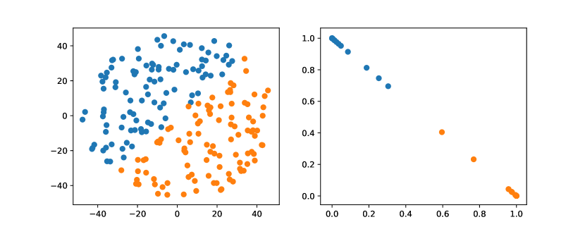
Figure 1: Softmax on an orthonormal basis

Similarly, figure 2 shows on the the same type of distribution of randomly selected values and the right shows the effect after a quasiorthonormal softmax is applied with three basis vectors. Since the qsoftmax function would map the two dimensional input into a three dimensional space, for graphics sake, the three dimensional vectors are mapped back down to two dimensions using the quasiorthonormal basis. Again with the exception of a few stragglers, most points move very close to one of the three basis vectors.

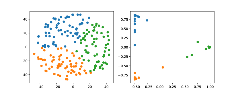
Figure 2: Softmax on a quasiorthogonal basis

It is clear from equation 3 that the exponential term in the numerator dominates which is why the softmax is effective. But consider if $\mathbf{z}\cdot\mathbf{u}_{i}$ is much less than zero such as $\mathbf{z}=-5\mathbf{u}_{i}$, then the exponential numerator for that term would severely attenuate the output even though the $\mathbf{z}$ lies along the same direction as $\mathbf{u}_{i}$. Since the $\mathbf{z}\cdot\mathbf{u}_{j}=0$ for all other j’s, it would still decode to $i$, but because the :math:i-th term is so small, any noise could lead to decoding to a different value.

So why bring all this up? Clearly, values encode to negative values along a basis vector would prove problematic. But it offers the prospect of further reducing dimensionality by encoding to no just the basis a vector but also its antipodal vector. To further our graphical example, in figure 3, we use $(1,0)$, $(0,1)$ and their antipodal vectors $(-1,0)$ and $(0,-1)$ to encode values and apply a softmax using those vectors.

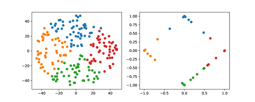
Figure 3: Softmax on encoded values using an orthonormal basis and antipodal points

Once again we see the power of the exponential term and most points move very close to one of the four encoding vectors.

Of course nothing comes for free, if a prediction gets confused between two antipodal unit vectors, the result could be that they cancel out and allow the noise to dictate the resulting category. By contrast, for one-hot encoding, the result would get decoded as one of the two possible values.

With this risk in mind, we can further extend the idea to a quasiorthogonal basis by adding the antipodal vectors for each vector in the basis. The result not only doubles the number of vectors that can be used for encoding, it reduces the problem of finding a basis to that of finding spherical codes.

Spherical Codes

Spherical codes can be used in place of quasiorthonormal codes simply by allowing the $\mathbf{q}_{i}$ to be a collection of spherical codes not necessarily quasiorthonormal basis. Table 11 shows how the example of the five Japanese car makes could be encoded with a simple spherical code.

Make	One-Hot	Spherical Code
Toyota	(1,0,0,0,0)	(1,0,0)
Honda	(0,1,0,0,0)	(-1,0,0)
Subaru	(0,0,1,0,0)	(0,1,0)
Nissan	(0,0,0,1,0)	(0,-1,0)
Mitsubishi	(0,0,0,0,1)	(0,0,1)

Table 12: Examples of Spherical Codes

Since spherical codes can substitute directly into the equations for QOE, it is a simple matter to implement spherical codes $\{\mathbf{s}_{i}\}$ instead of quasiorthonormal basis, $\{\mathbf{q}_{i}\}$. As such it is a simple matter to run the same experiment on the MNIST handwriting samples as we did for QOE. First, a set of codes are defined in an ndarray called code5 and code3. The variable code5 consists of the standard orthonormal basis in 5 dimensions along with their antipodal unit vector to produce a set of 10 vectors in 5 dimensions. The variable code3 is taken from [SHS20] for the 3 dimensional spherical codes with 10 vectors. Once these codes are defined, they can be substituted for basis4 and basis7 in the sample code above. Table 13 shows the results of the experiment with training accuracy shown in parentheses.

Number of	One Hot	5-Dimensional	3-Dimensional
Epochs	Encoding	Spherical Code	Spherical Code
10	97.53% (97.30%)	96.51% (96.26%)	95.37% (94.83%)
20	97.68% (98.02%)	96.82% (97.11%)	95.74% (95.83%)

Table 14: Results of MNIST Spherical Coding Experiment

In this case, the 5-dimensional spherical codes performed close to the one-hot encoding by not as closely as the 7-dimension QO codes. The 3-dimensional spherical codes performed on par with the 4-dimensional QO codes.

While the extreme dimensionality reduction from 10 to 4 or 10 to 3 did not yield comparable performance to one-hot encoding. More modest reductions such as 10 to 7 and 10 to 5 did. It is worth considering that quasiorthogonal or spherical codes are much harder to find in low dimensions. One should note that, though we went from 10 to 7 dimensions, we did not fully exploit the space spanned by the quasiorthogonal vector set. Otherwise, we would likely have had the similar results if the categorical labels had a cardinality of 28 rather than 10.

Conclusion

These reduced dimensionality codes are not expected to improve accuracy when the training data is plentiful, but to save computation and representation by reducing the dimensionality of the coded category. As an example, in application such as autoencoders and specifically the imputation architectures presented by [GW18] and [mLPU20] where the dimensionality not only dictates the number of outputs and inputs but also the number of hidden layers, a reduction in dimensionality has a profound impact on the size of the model used. Beyond that the reduced dimensionality codes such as QOE and spherical codes can address problems such as the curse of dimensionality and HDLSS where for small sample sizes it may improve accuracy.

Though for the exercises presented here, the reduction of dimensionality is modest and may not seem worth the trouble. The real benefit of these codes is in extremely high cardinality situations on the order of hundreds, thousands and beyond, such as zip codes, area codes, or medical diagnostic codes.

Practically speaking, while algorithms to generate spherical codes and quasiorthonormal sets are few, [SHS20] has a vast complication of spherical codes. At the extreme end, a spherical code with 196,560 vectors is available in 24 dimensions, enough to encode nearly 100,000 labels using QOE or 200,000 labels using spherical codes, in just 24 dimensions!

In sum, QOE and spherical codes are useful tools to be included in a data scientists tool box along side other established categorical coding techniques.

Experiments and code samples are made available at https://github.com/Westhealth/scipy2020/quasiorthonormal.

References

- [Ber18] Lucas Bernardi. Don’t be tricked by the hashing trick, Jan 2018. URL: https://booking.ai/dont-be-tricked-by-the-hashing-trick-192a6aae3087.
- [Eri20] Eric W. Weisstein. Spherical code. In From MathWorld- A Wolfram Resource, 2020. [Online; accessed 18-May-2020]. URL: https://mathworld.wolfram.com/SphericalCode.html.
- [GV13] Simanta Gautam and Dmitry Vaintrob. A novel approach to the spherical codes problem. 2013.
- [GW18] Lovedeep Gondara and Ke Wang. Mida: Multiple imputation using denoising autoencoders. In Dinh Phung, Vincent S. Tseng, Geoffrey I. Webb, Bao Ho, Mohadeseh Ganji, and Lida Rashidi, editors, Advances in Knowledge Discovery and Data Mining, pages 260–272, Cham, 2018. Springer International Publishing.
- [Hal18] Jeff Hale. Smarter ways to encode categorical data for machine learning: Exploring category encoders, Sep 2018. URL: https://towardsdatascience.com/smarter-ways-to-encode-categorical-data-for-machine-learning-part-1-of-3-6dca2f71b159.
- [Kai92] Paul Kainen. Orthogonal dimension and tolerance, 01 1992. URL: https://www.researchgate.net/publication/303520147.
- [KK96] V. Kůrková and P. C. Kainen. A geometric method to obtain error-correcting classification by neural networks with fewer hidden units. In Proceedings of International Conference on Neural Networks (ICNN’96), volume 2, pages 1227–1232 vol.2, 1996.
- [KK20] Paul C. Kainen and Věra Kůrková. Quasiorthogonal Dimension, pages 615–629. Springer International Publishing, Cham, 2020. URL: https://doi.org/10.1007/978-3-030-31041-7_35, doi:10.1007/978-3-030-31041-7_35.
- [LC10] Yann LeCun and Corinna Cortes. MNIST handwritten digit database. 2010. URL: http://yann.lecun.com/exdb/mnist/.
- [McG16] Will McGinnis. Category encoders, 2016. URL: http://contrib.scikit-learn.org/category_encoders/.
- [mLPU20] Haw minn Lu, Giancarlo Perrone, and José Unpingco. Multiple imputation with denoising autoencoder using metamorphic truth and imputation feedback, 2020. arXiv:2002.08338.
- [SHS20] N. J. A. Sloane, R. H. Hardin, and W. D. Smith. Spherical codes: Nice arrangements of points on a sphere in various dimensions, 2020. [Online; accessed 15-May-2020]. URL: http://neilsloane.com/packings/.
- [Ten19] Tensorflow. Tensorflow 2 quickstart for beginners, 2019. URL: https://www.tensorflow.org/tutorials/quickstart/beginner/.
- [Wik19] Wikipedia contributors. Steiner system — Wikipedia, the free encyclopedia, 2019. [Online; accessed 19-May-2020]. URL: https://en.wikipedia.org/w/index.php?title=Steiner_system&oldid=931308607.
- [Wik20a] Wikipedia contributors. Curse of dimensionality — Wikipedia, the free encyclopedia, 2020. [Online; accessed 15-May-2020]. URL: https://en.wikipedia.org/w/index.php?title=Curse_of_dimensionality&oldid=942360605.
- [Wik20b] Wikipedia contributors. Word embedding — Wikipedia, the free encyclopedia, 2020. [Online; accessed 16-May-2020]. URL: https://en.wikipedia.org/w/index.php?title=Word_embedding&oldid=951683288.