Geometrothermodynamics of black holes with a nonlinear source

Abstract

We study thermodynamics and geometrothermodynamics of a particular black hole configuration with a nonlinear source. We use the mass as fundamental equation, from which it follows that the curvature radius must be considered as a thermodynamic variable, leading to an extended equilibrium space. Using the formalism of geometrothermodynamics, we show that the geometric properties of the thermodynamic equilibrium space can be used to obtain information about thermodynamic interaction, critical points and phase transitions. We show that these results are compatible with the results obtained from classical black hole thermodynamics.

Keywords: Thermodynamics, Thermodynamic functions and equations of state, Phase transition, Riemannian geometries

I Introduction

Several regular black hole solutions have been found by coupling gravity to nonlinear electrodynamics theories. Among various regular models known to date, especially intriguing are the solutions to the coupled equations of nonlinear electrodynamics and general relativity Ayon2 ; Bronnikov . The description of magnetically charged black hole provides an interesting example of the system that could be both regular and extremal. In this same context are the theories of AdS-black holes that consider the so-called Power Maxwell Invariant (PMI) field Hassaine ; Hassaine2 ; Hendi0 ; Maeda where an $s$ parameter is introduced in order to represent a power term in the electromagnetic action, i.e. $(F_{\mu\nu}F^{\mu\nu})^{s}$, which reduces to Maxwellian field (linear electromagnetic source) when $s=1$. Nonlinear electrodynamic theories have been important at the low-energy limit of heterotic string theory or in the study of effects loop corrections in quantum electrodynamics Kats .

On the other hand, black hole thermodynamics has been the subject of numerous researches in theoretical physics. The main attraction lies in the fact that a black hole is the best system to seek the aspects of quantum gravity and it is expected that the thermodynamics of black holes help us to know about its microscopic structure. The norm/gravity correspondence introduced by Maldacena Maldacena , for example, considers the thermodynamic study of asymptoticaly AdS black holes relating black holes on the gravity side with the temperature on the field theory side. Hawking and Page’s research Hawking showed that black holes could be assigned entropy through which it is possible to study thermodynamic properties such as phase transitions and interaction; for example, the Reissner-Nordström-AdS (RNAdS) black hole in $n+1$ dimensions Chamblin1 , where it was found that it has phase transitions, or AdS black holes, where the cosmological constant is considered as a new thermodynamic variable Kastor Dolan1 . However, the full implication of the gravitational– thermodynamic connection is not yet apparent davies .

On the other hand, the geometric description of the thermodynamic properties of black holes has been investigated by using two different approaches, namely, Weinhold and Ruppeiner’s approach of thermodynamic geometry Weinhold ; Ruppeiner and the mathematical approach called geometrothermodynamics (GTD) quevedo2 . Both formalisms use a Riemannian manifold to define a space of equilibrium states where the thermodynamic phenomena take place; however, the Weinhold and Ruppeiner approaches are not Legendre inavariant, which implies that the properties of a given thermodynamic system can depend on the choice of thermodynamic potential. The formalism of GTD, on the contrary, is a geometric approach which considers the Legendre invariance and, therefore, describes the properties of the thermodynamic system independently of the thermodynamic potential, as in classical thermodynamics. In this work, we will use GTD in order to study the properties of black holes with a power Maxwell invariant field.

On the other hand, in black hole thermodynamics the degree of homogeneity of the fundamental equation is not always considered. The homogeneity of a thermodynamic system is very important because it allows us to know if the thermodynamic variables have a subextensive, extensive or supraextensive character. We show in this work how the GTD takes into account the homogeneity of the fundamental equation Quevedo5

This work is organized as follows. In Section II, we present the explicit form and review the main properties of a black hole with a power Maxwell invariant source, we analyze its fundamental equation and derive its main thermodynamic properties, considering the cosmological constant as an additional thermodynamic variable. In Section III, we perform a geometrothermodynamic analysis of the corresponding 3-dimensional equilibrium manifold, and show that its thermodynamic curvature leads to results which are equivalent to the ones obtained from the analysis of the corresponding heat capacity. This proves the compatibility between classical black hole thermodynamics and GTD. Finally, in Section IV, we present the conclusions of our work.

II Black holes with nolinear sources and theirs thermodynamics

The general action that describes Einstein-PMI gravity is given by the expression Hassaine2 ,

$$I=-\frac{1}{16\pi}\int_{M}{d^{n+1}x\sqrt{-g}\Big{[}R+\frac{n(n-1)}{l^{2}}+\Big{(}F_{\mu\nu}F^{\mu\nu}\Big{)}^{s}\Big{]}\,,}$$ (1)

where $F_{\mu\nu}$ represents the electromagnetic field tensor, $l$ is related to the cosmological constant by the expression $\Lambda=-\frac{3}{l^{2}}$ and $s$ is called nonlinearity parameter.

Considering a spherically symmetric spacetime with line element,

$$ds^{2}=-f(r)dt^{2}+\frac{dr}{f(r)}+r^{2}d\Omega^{2}{}_{d-2}\,,$$ (2)

where $d\Omega^{2}{}_{d-2}$ stands for the standard element on $S^{d}$. Using the equations obtained from the variation of the action (1), we get the next solution for a black hole with PMI source Hassaine ; Hendi

$$f(r)=1+\frac{r^{2}}{l^{2}}-\frac{m}{r{}^{n-2}}+\frac{(2s-1)^{2}\Big{[}\frac{(n-1)(2s-n)^{2}q^{2}}{(n-2)(2s-1)^{2}}\Big{]}^{s}}{(n-1)(n-2s)r{}^{\frac{2(ns-3s+1)}{2s-1}}}.$$ (3)

Here, $m$ and $q$ are related to the ADM mass $M$ and the electric charge $Q$ by means of the relation,

$$m = \frac{16\pi M}{(n-1)\omega_{n-1}}\,,$$ (4)

$$q = \Bigg{[}\frac{8\pi}{\sqrt{2}s\omega_{n-1}}\Bigg{]}^{\frac{1}{2s-1}}\Bigg{[}\frac{n-2}{n-1}\Bigg{]}^{\frac{1}{2}}\frac{(2s-1)^{\frac{2s-2}{2s-1}}}{n-2s}Q^{\frac{1}{2s-1}}.$$ (5)

The roots of the lapse function $f(r)$ ($g_{tt}=0$) define the horizons $r=r_{\pm}$ of the spacetime. In particular, the null hypersurface $r=r_{+}$ can be shown to correspond to an event horizon, which in this case is also a Killing horizon, whereas the inner horizon at $r_{-}$ is a Cauchy horizon. Therefore, from $f(r_{+})=0$ we get the black hole mass, $M$,

$$M(r_{+},Q)=\frac{(n-1)\omega_{n-1}}{16\pi}\Bigg{[}r_{+}{}^{n-2}+\frac{r_{+}{}^{n}}{l^{2}}-f_{n}r_{+}{}^{\frac{(2s-n)}{2s-1}}Q^{\frac{2s}{2s-1}}\Bigg{]}\,,$$ (6)

with

$$f_{n}=\frac{(2s-1)^{2-2s}(n-1)^{s-1}(2s-n)^{2s-1}}{(n-2)^{s}}\Bigg{[}\frac{8\pi}{\sqrt{2}s\omega_{n-1}}\Bigg{]}^{\frac{2s}{2s-1}}\Bigg{[}\frac{n-2}{n-1}\Bigg{]}^{s}\frac{(2s-1)^{\frac{2s(2s-2)}{2s-1}}}{(n-2s)^{2s}}\,.$$ (7)

From the area-entropy relationship, $S=\frac{\omega_{n-1}r_{+}{}^{n-1}}{4}$, equation (6) can be rewritten as

$$M(S,Q)=\frac{[4]^{\frac{n}{n-1}}(n-1)}{\pi}\omega_{n-1}^{\frac{1}{n-1}}\Bigg{[}S^{\frac{n-2}{n-1}}+S^{\frac{n}{n-1}}l^{-2}-\tilde{f}_{n}S^{\frac{2s-n}{(n-1)(2s-1)}}Q^{\frac{2s}{2s-1}}\Bigg{]},$$ (8)

where,

$$\tilde{f}_{n}=\Big{[}\frac{4}{\omega_{n-1}}\Big{]}^{\frac{6s-2sn-2}{(2s-1)(n-1)}}f_{n}\,,$$ (9)

with $\omega_{n-1}=(2\pi^{n/2})/\Gamma(n/2)$. In order to avoid inconsistent results, we will assume that $s>\frac{n}{2}$.

The equation (8) is the fundamental equation for black holes with PMI source. This equation relates all the thermodynamic variables entering the black hole metric. In order to correctly describe the thermodynamic properties of black holes, it is necessary to impose the condition that the corresponding fundamental equation be a quasi-homogeneous function Quevedo5 ; Quevedo6 . As we can observe, the fundamental equation (8) is an inhomogeneous function in the extensive variables $S$ and $Q$, e.i., the rescaling $S\rightarrow S\lambda^{\beta_{S}}$ and $Q\rightarrow Q\lambda^{\beta_{Q}}$ , where $\lambda$ and the $\beta$’s are real constants, does not fulfill the condition$M(\lambda^{\beta_{S}}S,\lambda^{\beta_{Q}}Q)=\lambda^{\beta_{M}}M(S,Q)$. However, if we consider $l$ also as a thermodynamic variable, which rescales as $l\rightarrow\lambda^{\beta_{l}}l$, the quasi-homogeneity condition $M(\lambda^{\beta_{S}}S,\lambda^{\beta_{Q}}Q,\lambda^{\beta_{l}}l)=\lambda^{\beta_{M}}M(S,Q,l)$ holds if the relationships,

$$\beta_{S}=\frac{n-1}{n-2}\,,\quad\quad\beta_{Q}=\frac{(2s-1)(n^{2}-2n-s+1)}{s(n-2)(2n-1)}\,,\quad\quad\beta_{l}=\frac{1}{n-2}\quad\quad\beta_{M}=1\,,$$ (10)

are fulfilled.

The physical parameters of the black hole with PMI source satisfy the first law of black hole thermodynamics davies ,

$$dM=TdS+\Phi dQ+Ldl\,,$$ (11)

where $T$ is the Hawking temperature, which is proportional to the surface gravity on the horizon, $\Phi$ is the electric potential and $L$ is the thermodynamic variable dual to $l$. The thermodynamic equilibrium conditions are given by the expressions,

$$T=\frac{\partial M}{\partial S}\,,\quad\quad\Phi=\frac{\partial M}{\partial Q}\,,\quad\quad L=\frac{\partial M}{\partial l}\,.$$ (12)

These expressions allow us to compute the explicit form of the corresponding intensive variables:

$$T = \Omega_{n}\Bigg{[}\frac{n-2}{n-1}S^{-\frac{1}{n-1}}+\frac{n}{n-1}\frac{S^{\frac{1}{n-1}}}{l^{2}}-\frac{(2s-n)\tilde{f}_{n}}{(n-1)(2s-1)}S^{\frac{4s-2sn-1}{(n-1)(2s-1)}}Q^{\frac{2s}{2s-1}}\Bigg{]}\,,$$ (13)

$$\Phi = -\frac{2s\Omega_{n}}{(2s-1)}\tilde{f}_{n}S^{\frac{2s-n}{(n-1)(2s-1)}}Q^{\frac{1}{2s-1}}\,,$$ (14)

$$L = -\frac{2\Omega_{n}}{l^{3}}S^{\frac{n}{(n-1)(2s-1)}}\,,$$ (15)

with $\Omega_{n}=\frac{[4]^{\frac{n}{n-1}}(n-1)}{\pi}\omega_{n-1}^{\frac{1}{n-1}}$. The behavior of the temperature $T$, electrical potential $\Phi$ and the thermodynamic variable $L$ in terms of the entropy $S$ is shown in Figures 1, 2, 3 y 4 for fixed values of the charge and the variable $l$.

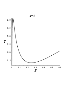
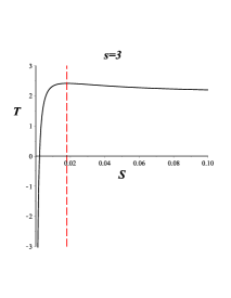
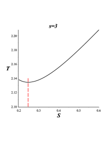
Figure 1: Temperature $T$ as a function of entropy $S$, where we have considered $n=4$, $l=Q=1$ and $s=3$.

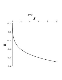
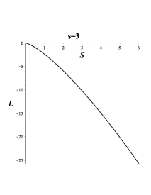
Figure 2: Electrical Potential (left) and the thermodynamic variable $L$ (right) as a function of entropy $S$, where we have considered $n=4$, $l=Q=1$ and $s=3$.

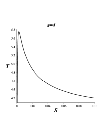
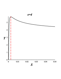
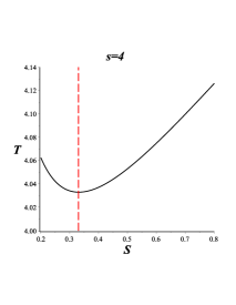
Figure 3: Temperature $T$ as a function of entropy $S$, where we have considered $n=5$, $l=Q=1$ and $s=4$.

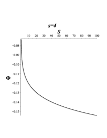
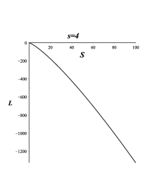
Figure 4: Electrical Potential (left) and the thermodynamic variable $L$ (right) as a function of entropy $S$, where we have considered $n=5$, $l=Q=1$ and $s=4$.

It is easy to show that the temperature (13 ) coincides with the Hawking temperature. The temperature increases rapidly as a function of the entropy $S$ until it reaches its maximum value. Then, as the entropy increases, the temperature becomes a monotonically decreasing function until it reaches another point from which the temperature increases again. The heat capacity at constant values of $Q$ and $l$ is computed by the expression,

$$C_{{}_{Q\,,l}}=T\Big{(}\frac{\partial S}{\partial T}\Big{)}_{Q\,,l}=\frac{\Big{(}\frac{\partial M}{\partial S}\Big{)}_{Q\,,l}}{\Big{(}\frac{\partial^{2}M}{\partial S^{2}}\Big{)}_{Q\,,l}}\,,$$ (16)

where the subscript indicates that derivatives are calculated keeping $Q$ and $l$ constants. The heat capacity that corresponds to the fundamental equation (8) is given by the expression

$$C_{{}_{Q\,,l}}=\frac{(n-1)\Big{[}l^{2}(2s-n)S^{\frac{4s-2ns-1}{(n-1)(2s-1)}}Q^{\frac{2s}{2s-1}}\tilde{f}_{n}-(2s-1)[(n-2)l^{2}+n]S^{-\frac{1}{(n-1)}}\Big{]}}{(2s-1)\Big{[}l^{2}(n-2)S^{-\frac{n}{(n-1)}}-nS^{-\frac{(n-2)}{(n-1)}}+\frac{(2s-n)(4s-2sn-1)}{(2s-1)^{2}}l^{2}\tilde{f}_{n}S^{\frac{6s-4ns+n-2}{(n-1)(2s-1)}}Q^{\frac{2s}{2s-1}}\Big{]}}\,,$$ (17)

According to Ehrenfest’s classification callen , second order phase transitions occur at those points where the heat capacity diverges, i.e., for

$$l^{2}(n-2)S^{-\frac{n}{(n-1)}}-nS^{-\frac{(n-2)}{(n-1)}}+\frac{(2s-n)(4s-2sn-1)}{(2s-1)^{2}}l^{2}\tilde{f}_{n}S^{\frac{6s-4ns+n-2}{(n-1)(2s-1)}}Q^{\frac{2s}{2s-1}}=0\,.$$ (18)

This behavior is depicted in figure 5

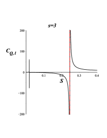
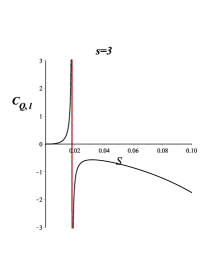
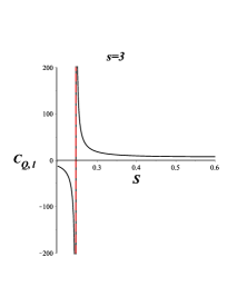
Figure 5: Heat Capacity $C_{Q\,,l}$ as a function of entropy $S$, where we have considered $n=4$, $l=Q=1$ and $s=3$.

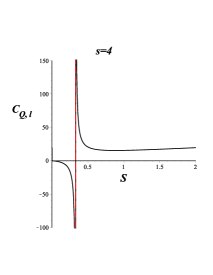
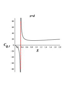
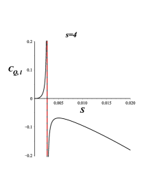
Figure 6: Heat Capacity $C_{Q\,,l}$ as a function of entropy $S$, where we have considered $n=5$, $l=Q=1$ and $s=4$.

We can see from the graphics 1,3,5 and 7 that in the region with positive temperature the heat capacity is positive, indicating that the black hole is stable in this region. At the maximum (minimum) value of the temperature, the heat capacity diverges and changes spontaneously its sign from positive to negative. This indicates the presence of second order phase transitions, which are accompanied by a transition into a region of instability.

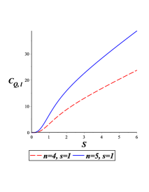
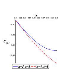
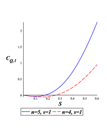
Figure 7: Heat Capacity $C_{Q\,,l}$ as a function of entropy $S$, where we have considered $n=4$, $l=Q=1$ and $s=1$.

On the other hand, figure 7 shows the behavior of the heat capacity for $s=1$, which corresponds to a black hole with linear electromagnetic source. As we can see, in the linear electromagnetic case there are no phase transitions. This shows that the nonlinearity of the electromagnetic source generate phase transitions.

III geometrothermodynamics formalism

In brief, GTD is a formalism based on a space which is a $(2n+1)-$ dimensional Riemannian contact manifold $(\mathcal{T},\Theta,G)$, where $\mathcal{T}$ represets a differential manifold, $\Theta$ is a contact form, i.e., $\Theta\wedge(d\Theta)^{n}\neq 0$, and $G$ a Riemannian metric. If we introduce in $\mathcal{T}$ the coordinates $Z^{A}=\{\Phi,E^{a},I^{a}\}$ with $a=1,...n$ and $A=0,...,2n$, according to Darboux theorem, the contact form $\Theta$ can be expressed as $\Theta=d\Phi-\delta_{ab}I^{a}dE^{b}$. On the other hand, the main ingredient of GTD is the Legendre invariance, which is considered through the metric $G$ demanding that it must be invariant with respect to Legendre transformations Arnold . In particular, three metrics have been found that are Legendre invariant Quevedo5 . One of them is used to describe the thermodynamics of black holes and can be written as

$$G=\Theta^{2}+(\delta_{ab}E^{a}I^{b})(\eta_{cd}dE^{c}dI^{d})\,,$$ (19)

where $\delta_{ab}={\mathrm{diag}}(1,1,\dots,1)$ and $\eta_{ab}={\mathrm{diag}}(-1,1,\dots,1)$. Using the metric (19) GTD induces a Legendre invariant metric $g$ on an $n-$ dimensional submanifold $\mathcal{E}\subset\mathcal{T}$ by mean of the pullback $\varphi^{*}(G)=g$, which is associated with the smooth embedding map $\varphi:\mathcal{E}\longrightarrow\mathcal{T}$ and fulfills the condition $\varphi^{*}(\Theta)=0$. If we choose the set $E^{a}$ as coordinates of $\mathcal{E}$, then the embedding reads $\varphi:\{E^{a}\}\longrightarrow\{\Phi(E^{a}),E^{a},I^{a}(E^{a})\}$ so that $\Phi(E^{a})$ is the fundamental equation and the induced metric becomes

$$g=\beta_{\Phi}\Phi\eta_{a}^{b}\Phi_{,bc}dE^{a}dE^{b}\,,$$ (20)

with $\Phi_{,a}=\frac{\partial\Phi}{\partial E^{a}}$, $\beta_{\Phi}$ is a constant and we have used the Euler identity in the form $\beta_{a}E^{a}\Phi_{,a}=\beta_{\Phi}\Phi$ for generalized homogeneous function Quevedo5 .

We now apply the above formalism to the case of black holes with PMI source. Let us consider the fundamental equation (8) which, according to the analysis presented above, is a generalized homogeneous function of degree 1 that does not involve a redefinition of the thermodynamic variables, affecting the physical properties of the thermodynamic system Quevedo5 . The thermodynamic metric (20) is 3-dimensional and reduces to

$$g = \frac{M[4]^{\frac{n}{n-1}}\omega_{n-1}^{\frac{1}{n-1}}}{\pi(n-1)}\Bigg{\{}\Big{[}(n-2)S^{-\frac{n}{n-1}}-\frac{n}{l^{2}}S^{-\frac{n-2}{n-1}}+$$ (21)

$$+ \frac{(2s-n)(4s-2sn-1)\tilde{f}_{n}}{(2s-1)^{2}}S^{-\frac{6s-4ns-n-2}{(n-1)(2s-1)}}Q^{\frac{2s}{2s-1}}\Big{]}dS^{2}-\frac{2s\tilde{f}_{n}}{(2s-1)^{2}}S^{\frac{2s-n}{(n-1)(2s-1)}}Q^{-\frac{2(s-1)}{2s-1}}dQ^{2}+$$

$$+ \frac{6}{l^{4}}S^{\frac{n}{(n-1)}}dl^{2}\Bigg{\}}\,.$$

The curvature scalar corresponding to the metric (21) takes the form,

$$R=\frac{N(S,Q,l)}{D_{1}D_{2}}\,,$$ (22)

where,

$$D_{1} = \Big{[}l^{2}(n-2)S^{-\frac{n}{(n-1)}}-nS^{-\frac{(n-2)}{(n-1)}}+\frac{(2s-n)(4s-2sn-1)}{(2s-1)^{2}}l^{2}\tilde{f}_{n}S^{\frac{6s-4ns+n-2}{(n-1)(2s-1)}}Q^{\frac{2s}{2s-1}}\Big{]}^{2}\,,$$ (23)

$$D_{2} = l^{2}S^{\frac{n-2}{n-1}}+S^{\frac{n}{n-1}}-l^{2}\tilde{f}_{n}S^{\frac{2s-n}{(n-1)(2s-1)}}Q^{\frac{2s}{2s-1}}\,,$$ (24)

and $N(S,Q,l)$ is a function that is different from zero at the points where denominator vanishes and cannot be written in a compact form. There are two curvature singularities in this case. The first one occurs if $D_{2}=0$ and corresponds to $M=0$, as follows from equation (8), see also figure 4. This means that this singularity is non physical since no black hole is present in this case. A second singularity is located at the roots of the equation $D_{1}=0$, it coincides with the points where $C_{Q,l}\longrightarrow\infty$, i. e., with the points where second order phase transitions take place. The general behavior of the curvature scalar is illustrated in figures 9 y 10.

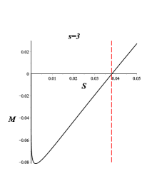
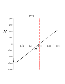
Figure 8: The mass $M$ as a function of the entropy $S$. We have considered $n=4$, $s=3$(left) and $n=5$, $s=4$(right), in both cases $l=Q=1$ and .

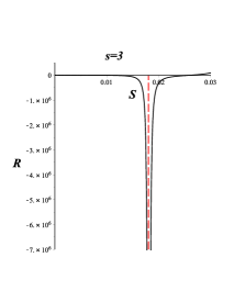
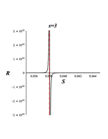
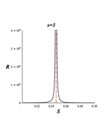
Figure 9: Behavior of the curvature scalar $R$, as a function of entropy $S$, for different intervals. We have considered $n=4$, $l=Q=1$ and $s=3$.

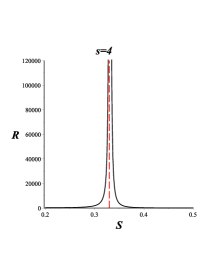
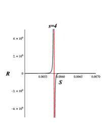
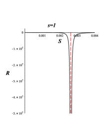
Figure 10: Behavior of the curvature scalar $R$, as a function of entropy $S$, for different intervals. We have considered $n=5$, $l=Q=1$ and $s=4$.

According to GTD, these results show that there exist curvature singularities at those points where second order phase transitions occur, because the denominators of the heat capacity and the curvature scalar coincide quevedo1 .

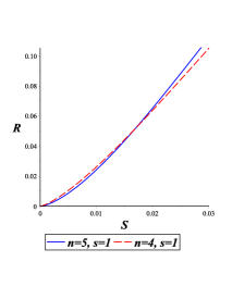
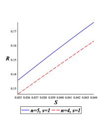
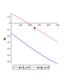
Figure 11: Behavior of the curvature scalar $R$, as a function of entropy $S$, for different intervals. We have considered $n=4$, $l=Q=1$ and $s=1$.

Figure 11 shows the behavior of the curvature scalar for a black hole with linear electromagnetic source ($s=1$). As we can see in the linear electromagnetic case there are no singularities. Therefore, GTD also reproduces correctly this case.

IV Conclusions

In this paper, we investigated the thermodynamics and geometrothermodynamics of a spherically symmetric AdS black hole with a PMI source. We analyzed the fundamental equation that relates the total mass, the entropy and charge. We showed that for the fundamental equation to be a generalized homogeneous function Quevedo5 , it is necessary to consider the variable $l$, related to the cosmological constant, as an extensive thermodynamic variable, in order for the fundamental equation to depend on extensive variables only. As a result, we obtained a fundamental equation whose mathematical properties resemble those of classical thermodynamic systems. Considering the curvature radius $l$ as an extensive thermodynamic variable implies that the equilibrium space must be extended by one dimension. A similar result was obtained recently Dolan , by assuming that the energy of a black hole is not represented by its total mass, but by the corresponding enthalpy, indicating that the cosmological constant is an intensive thermodynamic variable similar to the pressure. Our results corroborate from a more formal mathematical point of view the intuitive analysis performed in Dolan .

We investigated the properties of the extended 3-dimensional equilibrium space in the framework of GTD and we showed that in the space of equilibrium states of a black hole with PMI source, there exists a thermodynamic metric whose curvature turns out to be nonzero, indicating the presence of thermodynamic interaction. We also found that the curvature is singular at those points where phase transitions of the heat capacity occur. This has been shown by considering a particular metric in the thermodynamic phase space, and applying the formalism of geometrothermodynamics. An important property of our choice of thermodynamic metric is that it is invariant with respect to Legendre transformations so that the properties of our geometric description of thermodynamics are independent of the choice of thermodynamic potential and representation.

We conclude that the thermodynamic properties of this particular class of a black holes with no linear source are correctly described within the GTD formalism.

References

- (1) E. Ayon-Beato and A. Garcia, Phys. Lett. B 464, 25 (1999).
- (2) K. A. Bronnikov, Phys. Rev. D63, 044005 (2001)
- (3) M. Hassaine and C. Martinez, Class. Quantum Gravit. 25, 195023 (2008)
- (4) M. Hassaine and C. Martinez, Phys. Rev. D 75, 027502 (2007).
- (5) S. H. Hendi and H. R. Rastegar-Sedehi, Gen. Rel. Grav. 41, 1355 (2009).
- (6) H. Maeda, M. Hassaine and C. Martinez, JHEP 1008, 123 (2010).
- (7) Y. Kats, L. Motl and M. Padi, JHEP 0712, 068 (2007);
- (8) J. M. Maldacena, AIP Conf. Proc. 484, 51 (1999) [Int. J. Theor. Phys. 38, 1113 (1999)].
- (9) S. W. Hawking and D. N. Page, Commun. Math. Phys. 87, 577 (1983).
- (10) A. Chamblin, R. Emparan, C. V. Johnson and R. C. Myers, Phys. Rev. D 60, 064018 (1999).
- (11) D. Kastor, S. Ray and J. Traschen, Class. Quant. Grav. 26, 195011 (2009).
- (12) B. P. Dolan, Class. Quant. Grav. 28, 125020 (2011).
- (13) P. C. W. Davies, Proc. Roy. Soc. Lond. A 353, 499 (1977).
- (14) F. Weinhold, J. Chem. Phys. 63, 2479, 2484, 2488, 2496 (1975); 65, 558 (1976).
- (15) G. Ruppeiner, Phys. Rev. A 20, 1608 (1979).
- (16) H. Quevedo, J. Math. Phys. 48, 013506 (2007).
- (17) S. H. Hendi and M. H. Vahidinia, Phys. Rev. D 88, 084045 (2013).
- (18) H. Quevedo, M. N. Quevedo, and A. S nchez, Eur. Phys. J. C 77, 158 (2017).
- (19) H. Quevedo, M. N. Quevedo, and A. Sánchez,Eur. Phys. J. C (2019) 79:229.
- (20) H.B. Callen,Thermodinamics (John Wiley and Sons, Inc., New York, 1981), pag. 132.
- (21) V. I. Arnold, Mathematical Methods of Classical Mechanics (Springer Verlag, New York, 1980).
- (22) H. Quevedo, A. Sanchez, S. Taj and A. Vazquez, Gen. Rel. Grav. 43, 1153 (2011).
- (23) B. P. Dolan, Where is the PdV term in the first law of black hole thermodynamics?, arXiv:1209.1272 [gr-qc](2016).