Black Hole Metamorphosis
and Stabilization by Memory Burden

Abstract

Systems of enhanced memory capacity are subjected to a universal effect of memory burden, which suppresses their decay. In this paper, we study a prototype model to show that memory burden can be overcome by rewriting stored quantum information from one set of degrees of freedom to another one. However, due to a suppressed rate of rewriting, the evolution becomes extremely slow compared to the initial stage. Applied to black holes, this predicts a metamorphosis, including a drastic deviation from Hawking evaporation, at the latest after losing half of the mass. This raises a tantalizing question about the fate of a black hole. As two likely options, it can either become extremely long lived or decay via a new classical instability into gravitational lumps. The first option would open up a new window for small primordial black holes as viable dark matter candidates.

I Introduction

I.1 Big Picture

This paper is about understanding a very general phenomenon [1, 2], called memory burden, exhibited by systems that achieve a high capacity of memory storage and its potential applications to black holes. The essence of the story is that a high load of quantum information carried by such a system stabilizes it. This means that, in order to decay, the system must off-load the memory pattern from one set of modes into another one. Our studies show that this becomes harder and harder with larger size. As a result, the quantum information stored in the memory back-reacts and stabilizes the system at the latest after its half-decay. The universality of the phenomenon suggests its natural application to black holes.

The present paper is a part of a general program, initiated some time ago, which consists of two main directions. One is the development of a microscopic theory describing a black hole as a bound state of soft gravitons, a so-called quantum $N$-portrait [3]. The occupation number $N_{c}$ of gravitons is critical in the sense that it is the inverse of their (dimensionless) gravitational interaction. The softness of gravitons here refers to wavelengths comparable to the gravitational radius of a black hole. This criticality has been identified [4] as the key reason for understanding the maximal information storage capacity of a black hole quantified by its Bekenstein-Hawking entropy. Due to extremely weak interactions among the constituent gravitons, this framework allows to perform computations within the validity domain of effective field theory exploiting the power of $1/N_{c}$-expansions.

The second direction [4, 5, 6, 7, 8, 9, 10, 11, 1, 2, 12, 13, 14] is to instead use the enhanced capacity of memory storage as a guiding principle. That is, we study generic systems which possess states with a high capacity of memory storage and try to identify universal phenomena that take place near such states. The idea then is to come back and apply this knowledge to black holes and look for analogous phenomena there. The advantage of this approach is that a unique knowledge about black holes can be gained by studying systems that are much easier solvable both analytically and numerically. The present paper is about the detailed study of one such universal phenomenon identified in [1, 2], namely the above mentioned memory burden.

Before continuing we wish to make a clarifying remark, in order not to confuse the reader with our terminology. We shall often use the term enhanced capacity of the memory storage as opposed to, for example, maximal entropy. This is because the former term covers a wider class of systems: A state can have a sharply enhanced memory storage capacity even if the corresponding microstate entropy is not necessarily maximal. The above studies show that systems that possess such states still exhibit some black hole like properties. Of course, the converse is in general true: A state of maximal microstate entropy does possess a maximal memory storage capacity. In particular, all such states must share the memory burden effect.

I.2 Main Finding

Let us start with setting the framework. Physical systems are characterized by a set of degrees of freedom (modes) and interactions between them. It is convenient and customary to describe the degrees of freedom as quantum oscillators. The basic quantum states of the system then can be labeled by a sequence of their occupation numbers $\ket{n_{1},\ldots,n_{K}}$. Such a sequence stores quantum information which we can refer to as the memory pattern. The efficiency of memory storage is then measured by the number of patterns that can be stored within a certain microscopic energy gap [9, 11]. When this number is high, we shall say that the system has an enhanced capacity of memory storage. The above notion is closely related to microstate entropy but is much more general. If the states describing different patterns share the same macroscopic characteristics (e.g., the total mass or angular momentum), the microstate entropy can be defined in the usual way $S=\ln(n_{\rm st})$, where $n_{\rm st}$ is the number of distinct basic microstates $\ket{n_{1},\ldots,n_{K}}$.

Naturally, we are interested in systems that dynamically attain a high capacity of memory storage. This can be achieved if the system reaches a critical state in which a large number of gapless modes emerge. Then information can be encoded in the occupation numbers of the gapless modes without energy cost. This generic mechanism has already been investigated in a series of papers [4, 5, 8, 9, 10, 11, 1, 2]. Originally, it was introduced for understanding the origin of Bekenstein-Hawking entropy in a microscopic theory of black hole’s quantum $N$-portrait [3]. However, it was soon realized in the above papers that this mechanism is universally operative in systems with high capacity of memory storage. Interestingly, it has been repeatedly observed that the information storage in such systems exhibits some black hole-like properties.

This universality suggests that by understanding general phenomena and applying this understanding to black holes, we can gain new knowledge that until now has been completely blurred by technical difficulties in quantum gravity computations. Such terra incognita is the black hole evolution beyond its half evaporation. The reason is that the standard semi-classical computations are unable to account for quantum back reaction. Therefore, they are no longer applicable once back reaction becomes important, i.e., the latest by half evaporation. Instead, for resolving such questions a microscopic theory is needed such as quantum $N$-portrait [3].

As mentioned above, in this microscopic theory the black hole is described as a saturated critical state of soft gravitons of wavelengths given by the gravitational radius of a black hole, $r_{g}$. Since the occupation number is critical, i.e., equal to the inverse of their gravitational coupling, the kinetic energy of individual gravitons just saturates the collective attraction from the rest. As a result, the gravitons form a long-lived bound-state, a black hole. However, the bound-state is not eternal. Instead, due to their quantum re-scattering, the soft bound-state slowly loses its constituents and depletes. On average, it emits a quantum of wavelength $r_{g}$ per time $r_{g}$. At the same time, the emissions of quanta that are either much harder or softer are suppressed. In total, this process reproduces Hawking’s evaporation up to $1/N_{c}$ corrections. It is these $1/N_{c}$-corrections that are responsible for new effects that were invisible in the standard semi-classical treatment. Note that the latter corresponds to the $N_{c}=\infty$ limit of the microscopic theory.

The computations performed in the microscopic theory [15, 16, 17, 18, 19] unambiguously indicate that the classical description breaks down after the black hole has lost on the order of half of its mass, which corresponds to on the order of $N_{c}/2$ emissions. At this point, the back reaction (i.e., $1/N_{c}$-effects integrated over time) become so important that the true quantum evolution completely departs from the naive semi-classical one. In this light, the two immediate tasks are: 1) Better quantify the quantum back reaction effects that lead to this breakdown; and 2) Predict what happens beyond this point.

In order to address these questions, we shall try to understand very general aspects of time-evolution of systems of enhanced memory capacity. We shall use the simplest possible prototype model with this property. Then we try to extend the obtained knowledge to black holes and cosmology and speculate about the possible consequences. The above strategy is the continuation of the one adopted in the previous papers [4, 5, 6, 7, 8, 9, 10, 11, 1, 2, 12, 13, 14]. The persistent pattern emerging from this work is that systems of enhanced capacity of memory storage exhibit striking similarities with certain black hole properties. For example, they share a slow initial decay via the emission of the soft quanta without releasing the stored information for a very long time. In short, it appears to be a promising strategy to try to make progress in understanding black holes by abstracting from the geometry and instead viewing their information storage capacity as the key characteristic.

In order to avoid any misunderstanding, we wish to clearly separate solid results from speculations. In the present paper, we shall focus on a very precise source of quantum back reaction. Following [1, 2], we shall refer to it as the phenomenon of memory burden. The essence of it, as described above, is that the high load of quantum information stored in a memory pattern tends to stabilize the system in the state of enhanced memory capacity. We shall show that the strength of the effect maximizes at the latest by the time the system emits half of its energy. At the same time, the information stored in the memory becomes accessible. Because of very transparent physical mechanism behind these findings, it is almost obvious that it must be shared by generic systems of enhanced memory capacity, including black holes and de Sitter Hubble patch. This means that the tendency of a growing back reaction from the memory burden must be applicable to such objects. It is therefore expected that the back reaction from a stored quantum information must drastically modify the semi-classical picture by half-decay.

Note that this statement is in no conflict with any known black hole property derived in semi-classical theory. The reason, as already predicted both by calculations in gravitational microscopic theory [15, 16, 17, 18, 19] as well as by analysis of the prototype models [4, 5, 6, 7, 8, 9, 10, 11, 1, 2, 12, 13, 14] including the present paper, is that after losing half of the mass the semi-classical description is no longer applicable. Namely:

An old black hole that lost half of its mass is by no means equivalent to a young classical black hole of the equal mass.

In other words, the quantum effects such as the memory burden provide a universal quantum clock that breaks the self-similarity of black hole evaporation and suppresses its quantum decay. This is the key result of the present paper.

Some applications of this phenomenon to inflationary cosmology were already discussed in [2]. It was pointed out there that the memory burden of the primordial information carried by degrees of freedom responsible for Gibbons-Hawking entropy [20] can provide a new type of the cosmic quantum hair. This hair imprints a primordial quantum information from the early stages of inflation past last the $60$ e-foldings.

Now, the speculative part of our paper concerns the extrapolation of the stabilization tendency for a black hole beyond its half-decay. At the present level of understanding, such an extrapolation is a pure speculation since strictly speaking there is no guarantee that universality of the phenomenon holds on such long timescales. In particular, it remains a viable option that after losing on the order of half of its mass via quantum emission, a new classical instability can set in. The black hole then can fall apart via a highly non-linear classical process.

Our precautions can be explained in the following way. The state of maximal memory capacity represents a type of criticality. The behavior of the system is then fully controlled by the gapless spectrum that emerges in this state. This explains the universal behavior of very different systems that exist in such a state. However, after half-decay the departure from the critical state is significant and it is conceivable that different systems behave differently after this point. So, despite the fact that our prototype model gets stabilized, a real black hole could follow a different path.

In summary, the following two natural possibilities emerge:

• The black hole continues its quantum decay but with an extremely-suppressed emission rate.

• A classical instability sets in and the black hole decays into highly non-linear graviton lumps, a sort of a gravitational burst.

While both outcomes would obviously have spectacular consequences, in the present paper we shall speculate more on the first option. That is, we can take the stabilization exhibited by the prototype model as a circumstantial evidence indicating that large black holes (i.e., $N_{c}\gg 1$, meaning much heavier than the Planck mass) behave in a similar manner, at least qualitatively. Therefore, the decay rate of macroscopic black holes could fall drastically after they lose half of their mass. Not surprisingly, the consequences of such stabilization would be dramatic. One obvious application that shall be discussed later is for primordial black holes as dark matter candidates.

I.3 Outline

We shall now briefly outline our analysis in more technical terms. The first ingredient is to explain the essence of the universal mechanism which allows the system to reach the state of enhanced memory storage. This mechanism is at work in large class of systems [4, 5, 6, 7, 8, 9, 10, 11, 1, 2]. Following [11], we shall refer to it as assisted gaplessness. The essence of this mechanism is most transparently explained by a simple model discussed in [8, 9, 10, 1, 2], which we shall adopt as the prototype system in our analysis. The idea is that a high occupation of a particular low-frequency mode to a certain critical level, renders a large set of other would-be-high-frequency modes gapless. Namely, the highly-occupied master mode interacts attractively with a set of other modes. We shall call the latter degrees of freedom the memory modes. Near the vacuum, the memory modes would have high energy gaps and would be useless (i.e., energetically costly) for storing information. However, coupling to the master mode lowers their energy gaps when the latter is highly occupied. That is, the attractive coupling with the master mode translates as a negative contribution to the energy of the memory modes. As soon as the occupation number of the master mode reaches a critical level $N_{c}$, it can balance their positive kinetic energies. In this way, the memory modes become effectively gapless. Consequently, the states that correspond to different occupation numbers of these modes, $\ket{n_{1},\ldots,n_{K}}$, are degenerate in energy and contribute into the microstate entropy $S$.

So far, we have discussed how the master mode influences the memory modes by making them effectively gapless. However, the memory modes also backreact on the master mode via the effect of memory burden [1, 2]. Since the memory modes are gapless exclusively for a critical occupation $N_{c}$ of the master mode, any evolution of the latter away from such a state would cost a lot of energy. Therefore, the system backreacts on the master mode and resists to the change of its occupation number $N_{c}$.

The next step in this line of research is to study to what extent the memory burden can be avoided. Namely, it has been proposed in [1] that it can be alleviated if the system has a possibility of rewriting the stored information from one set of modes to another. This could happen if another set of memory modes exists, which becomes gapless at a different occupation number $N^{\prime}_{c}$ of the master mode. Then, it is in principle conceivable that the occupation $N_{c}$ changes in time, provided this change is accompanied by rewriting of the stored information from the first set of the memory modes to the second one. However, it has not yet been studied if such a rewriting is dynamically possible.

In order to attack the issue, we can split this question in two parts.

1. Does rewriting take place at all and under what conditions?

2. If the answer to the first question is positive, what is the timescale of this process?

Answering these questions is the goal of the present work.

In section II, we will summarize some of the findings of [4, 5, 6, 7, 8, 9, 10, 11, 1, 2] and develop a concrete prototype model that possesses states of enhanced memory capacity. Moreover, we discuss how it can be mapped on a black hole. In section III, we investigate the prototype model numerically and in particular study rewriting between two different sets of memory modes. In short, we confirm that such a possibility can be realized dynamically. However, we discover that the speed of transition decreases as the size of the system increases. Applied to black holes, this indicates that evaporation has to slow down at the latest after they have lost half of their mass. In section IV, we briefly discuss systems that do not conserve particle number and point out that our conclusions also apply to them. Section V is dedicated to studying consequences of our findings for primordial black holes as dark matter candidates. We give an outlook in section VI and the appendix contains details as to how the speed of rewriting depends on the various parameters of the system.

II Enhanced Memory Storage: A Prototype Model

II.1 Assisted Gaplessness

Following [10, 9, 11], we shall construct a simple prototype model that dynamically achieves a state with many gapless modes and correspondingly a high microstate entropy $S$. We consider $K$ bosonic modes, which we describe by the usual creation and annihilation operators $\hat{a}_{k}^{\dagger}$, $\hat{a}_{k}$, where $k=1,\ldots K$. They satisfy standard commutation relations (here and throughout $\hbar=1$):

$$[\hat{a}_{j},\hat{a}_{k}^{\dagger}]=\delta_{jk}\,,\qquad[\hat{a}_{j},\hat{a}_{k}]=[\hat{a}_{j}^{\dagger},\hat{a}_{k}^{\dagger}]=0\,,$$ (1)

and the corresponding number operators are given as $\hat{n}_{k}=\hat{a}_{k}^{\dagger}\hat{a}_{k}$. We denote its eigenstates by $\ket{n_{k}}$, where $n_{k}$ is the eigenvalue. Moreover, we label the energy gap of $\hat{n}_{k}$ by $\epsilon_{k}$.

Using the modes $\hat{n}_{k}$, one can form the states

$$\ket{n_{1},\ldots,n_{K}}\equiv\ket{n_{1}}\otimes\ket{n_{2}}\otimes,\ldots,\otimes\ket{n_{K}}\,,$$ (2)

where $n_{1},\ldots n_{K}$ can take arbitrary values. Clearly, the number of such states scales exponentially with $K$, so for $K\gtrsim S$, their number reaches the required number of microstates. However, it is important to consider the energy of the states (2). Namely, two different states $\ket{n_{1},\ldots n_{S}}$ and $\ket{n^{\prime}_{1},\ldots n^{\prime}_{S}}$ differ by the energy $\Delta E=\sum_{k=1}^{K}\epsilon_{k}(n_{k}-n^{\prime}_{k})$. So unless the $\epsilon_{k}$ are extremely small, the states corresponding to different occupation numbers of the modes $\hat{n}_{k}$ are not degenerate in energy. Therefore, they cannot contribute to a microstate entropy.

We can change this situation by introducing another mode $\hat{n}_{0}$, with creation and annihilation operators $\hat{a}_{0}^{\dagger}$, $\hat{a}_{0}$ and commutation relations analogous to Eq. (1). The key point is that we add an attractive interaction between the mode $\hat{n}_{0}$ and all other modes:

$$\hat{H}=\epsilon_{0}\hat{n}_{0}+\left(1-\frac{\hat{n}_{0}}{N_{c}}\right)\sum_{k=1}^{K}\epsilon_{k}\hat{n}_{k}\,,$$ (3)

where we parameterize the strength of the interaction by $1/N_{c}$ with $N_{c}\gg 1$. As long as $\hat{n}_{0}$ is not occupied, the gaps of the $\hat{n}_{k}$-modes are still given by $\epsilon_{k}$. As soon as we populate $\hat{n}_{0}$, however, the effective gaps $\mathcal{E}_{k}$ of the $\hat{n}_{k}$-modes are lowered:

$$\mathcal{E}_{k}=\left(1-\frac{n_{0}}{N_{c}}\right)\epsilon_{k}\,.$$ (4)

Once a critical occupation $n_{0}=N_{c}$ is reached, all modes $\hat{n}_{k}$ become effectively gapless, $\mathcal{E}_{k}=0$.

Therefore, all states of the form

$$\ket{\underbrace{N_{c}}_{n_{0}},n_{1},\ldots,n_{K}}$$ (5)

are degenerate in energy for arbitrary values of $n_{1}$, …, $n_{K}$. In this situation, $\hat{n}_{0}$ is the master mode, which assists the memory modes $\hat{n}_{1}$, …, $\hat{n}_{K}$ in becoming gapless. We note, however, that one has to invest the energy $\epsilon_{0}N_{c}$ to achieve gaplessness. If each of the memory modes can have a maximal occupation of $d$, this leads to a number of $(d+1)^{K}$ distinct states that possess the same energy, i.e., an entropy

$$S=K\ln(d+1)\,.$$ (6)

In this way, a large number $K\approx S$ of nearly-gapless modes leads to the entropy $S$.

II.2 Memory Burden

Following [1, 2], we next investigate the effect of memory burden, i.e., how the memory modes backreact on the master mode. To this end, we add another mode with which $\hat{n}_{0}$ can exchange occupation number. We denote its creation and annihilation operators by $\hat{b}_{0}^{\dagger}$, $\hat{b}_{0}$ with commutation relations analogous to Eq. (1) and $\hat{m}_{0}=\hat{b}_{0}^{\dagger}\hat{b}_{0}$ is the corresponding number operator. Then the Hamiltonian becomes

$$\hat{H}=\epsilon_{0}\hat{n}_{0}+\epsilon_{0}\hat{m}_{0}+\left(1-\frac{\hat{n}_{0}}{N_{c}}\right)\sum_{k=1}^{K}\epsilon_{k}\hat{n}_{k}+C_{0}\left(\hat{a}_{0}^{\dagger}\hat{b}_{0}+\hat{b}_{0}^{\dagger}\hat{a}_{0}\right)\,,$$ (7)

where $C_{0}$ parametrizes the strength of interaction between $\hat{n}_{0}$ and $\hat{m}_{0}$. We choose the gap of $\hat{n}_{0}$ and $\hat{m}_{0}$ to be equal in order to facilitate the oscillations between them.

Now we consider the initial state

$$\ket{\text{in}_{1}}=\ket{\underbrace{N_{c}}_{n_{0}},\underbrace{0}_{m_{0}},n_{1},\ldots,n_{K}}\,.$$ (8)

Since the occupation number of each of the memory modes is conserved in time, it is possible to solve the system analytically. For the expectation value of $\hat{n}_{0}$, one obtains [1]:

$$n_{0}(t)=N_{c}\left(1-\frac{4C_{0}^{2}}{4C_{0}^{2}+\mu^{2}}\sin^{2}(\sqrt{C_{0}^{2}+\mu^{2}/4}\,t)\right)\,,$$ (9)

where we defined

$$\mu=-\sum_{k=1}^{K}\epsilon_{k}n_{k}/N_{c}\,.$$ (10)

This quantity characterizes the strength of memory burden, as we shall demonstrate. It is related to the effective energy gaps (4) as

$$\mu=\sum_{k=1}^{K}n_{k}\frac{\partial\mathcal{E}_{k}}{\partial n_{0}}\,.$$ (11)

Eq. (9) shows that the memory modes drastically influence the time evolution of $\hat{n}_{0}$. First, we consider the special situation in which all memory modes are unoccupied. This implies $\mu=0$ so that $n_{0}(t)$ performs oscillation with maximal amplitude on a timescale of $C_{0}^{-1}$. This behavior, which is depicted in Fig. 1(a), is identical to the case in which the memory modes do not exist. For $n_{k}\neq 0$, this situation changes as soon as either the occupation of the memory modes is high enough or their free gaps $\epsilon_{k}$ are sufficiently big. In both cases, one gets $C_{0}^{2}/\mu^{2}\ll 1$ so that the amplitude of oscillations is suppressed by this ratio. This is shown in Fig. 1(b) for exemplary values of the parameters. Thus, the stored information ties $\hat{n}_{0}$ to its initial state. This is the essence of memory burden.

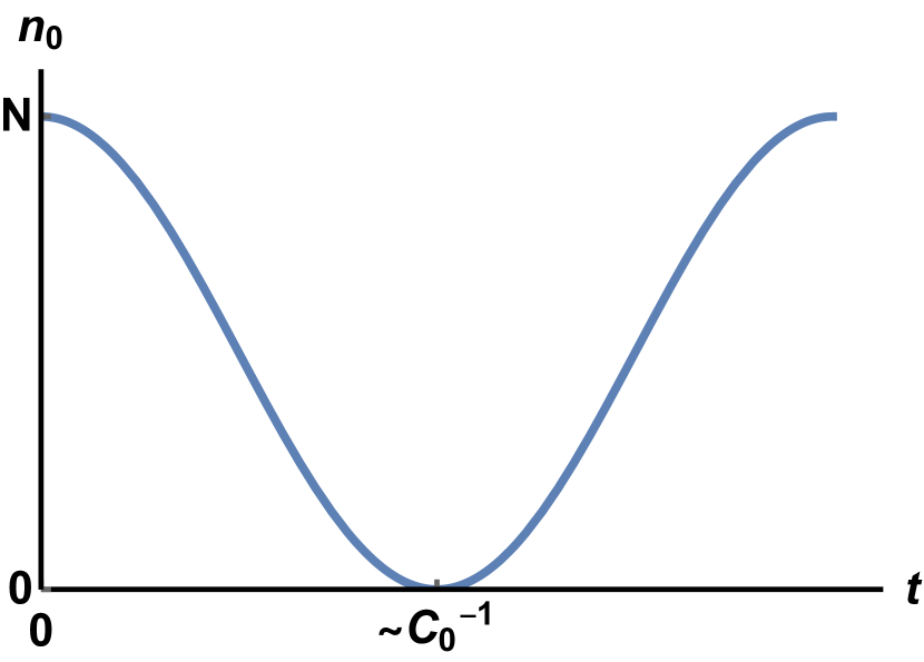
(a) $\mu=0$: absence of memory burden. The expectation value $n_{0}$ oscillates freely with full amplitude.

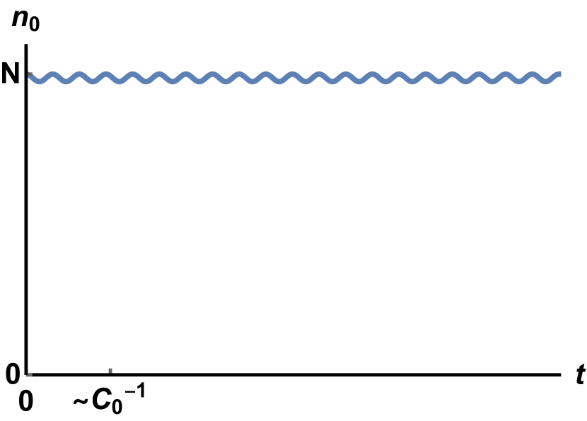
(b) $|\mu|\ =2.5$ (and $p=1$): early backreaction due to memory burden ties $n_{0}$ to its initial value.

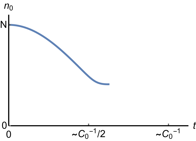
(c) $|\mu|\ =2.5$ and $p=8$: memory burden can be delayed up to a timescale on the order of half decay. Backreaction sets in at the latest at that point and stabilizes the system.

Figure 1: Plots of the time evolution of $n_{0}$ for $N_{c}=25$ and $C_{0}=\epsilon_{0}/\sqrt{N_{c}}=1/5$. Figs. 1(a) and 1(b) follow from (9). Fig. 1(c) is an approximate solution of the system (12).

Consequently, the crucial question arises to what extent memory burden can be avoided. Following [2], a first way consists in modifying the Hamiltonian (7) as follows:

$$\hat{H}=\epsilon_{0}\hat{n}_{0}+\epsilon_{0}\hat{m}_{0}+\left(1-\frac{\hat{n}_{0}}{N_{c}}\right)^{p}\sum_{k=1}^{K}\epsilon_{k}\hat{n}_{k}+C_{0}\left(\hat{a}_{0}^{\dagger}\hat{b}_{0}+\hat{b}_{0}^{\dagger}\hat{a}_{0}\right)\,.$$ (12)

In this case, the effective energy gaps read

$$\tilde{\mathcal{E}}_{k}=\left(1-\frac{n_{0}}{N_{c}}\right)^{p}\epsilon_{k}\,.$$ (13)

Consequently, the memory burden becomes

$$\tilde{\mu}=p\left(\frac{N_{c}-n_{0}}{N_{c}}\right)^{p-1}\mu\,,$$ (14)

where we expressed it in terms of Eq. (10). We see that it gets suppressed by powers of $(N_{c}-n_{0})/N_{c}$. The larger $p$ is, the more the backreaction gets delayed. However, it sets in at the latest when $\tilde{\mu}$ assumes the critical value $C_{0}$:

$$N_{c}-n_{0}=N_{c}\left(\frac{C_{0}}{p|\mu|}\right)^{1/(p-1)}\,.$$ (15)

For $\mu>C_{0}$, it is clear that memory burden can no longer be avoided as soon as $N_{c}-n_{0}$ is of the order of $N_{c}$. Thus, backreaction becomes important and the system stabilizes at the latest after a timescale on the order of half decay, as is exemplified in Fig. 1(c).

II.3 Avoiding Memory Burden by Rewriting

In [1], another way of alleviating memory burden was proposed. The idea is to introduce a second sector of memory modes, which are not occupied in the beginning, but which can exchange occupation number with the first sector. If the coupling of the second sector to the master mode is such that it becomes gapless for a smaller value $n_{0}=N_{c}-\Delta N_{c}$, then a final state in which $n_{0}$ has diminished by $\Delta N_{c}$ and all excitations have been transferred from the first to the second memory sector becomes energetically available.

We denote the creation and annihilation operators of the second memory sector by $\hat{a}^{{}^{\prime}\dagger}_{k^{\prime}}$, $\hat{a}^{{}^{\prime}}_{k^{\prime}}$, the number operator by $\hat{n}^{\prime}_{k^{\prime}}=\hat{a}^{{}^{\prime}\dagger}_{k^{\prime}}\hat{a}^{{}^{\prime}}_{k^{\prime}}$ and assume the usual commutation relations (1), where $k^{\prime}=1,\ldots,K^{\prime}$. Then the Hamiltonian becomes:

$$\hat{H} =\epsilon_{0}\hat{n}_{0}+\epsilon_{0}\hat{m}_{0}+C_{0}\left(\hat{a}_{0}^{\dagger}\hat{b}_{0}+\hat{b}_{0}^{\dagger}\hat{a}_{0}\right)$$

$$+\left(1-\frac{\hat{n}_{0}}{N_{c}}\right)\sum_{k=1}^{K}\epsilon_{k}\hat{n}_{k}+\left(1-\frac{\hat{n}_{0}}{N_{c}-\Delta N_{c}}\right)\sum_{k^{\prime}=1}^{K^{\prime}}\epsilon_{k^{\prime}}\hat{n}^{\prime}_{k^{\prime}}$$

$$+\sum_{k=1}^{K}\sum_{k^{\prime}=1}^{K^{\prime}}C_{k,k^{\prime}}\left(\hat{a}_{k}^{\dagger}\hat{a}^{\prime}_{k^{\prime}}+\text{h.c.}\right)$$

$$+\sum_{k=1}^{K}\sum_{\begin{subarray}{c}l=1\\ l>k\end{subarray}}^{K}\tilde{C}_{k,l}\left(\hat{a}_{k}^{\dagger}\hat{a}_{l}+\text{h.c.}\right)$$

$$+\sum_{k^{\prime}=1}^{K^{\prime}}\sum_{\begin{subarray}{c}l^{\prime}=1\\ l^{\prime}>k^{\prime}\end{subarray}}^{K^{\prime}}\tilde{C}_{k^{\prime},l^{\prime}}\left(\hat{a}_{k^{\prime}}^{{}^{\prime}\dagger}\hat{a}^{\prime}_{l^{\prime}}+\text{h.c.}\right)\,.$$ (16)

Here the parameters $C_{k,k^{\prime}}$ determine the strength of coupling between the two memory sectors. For completeness, we have moreover introduced interactions within each memory sector, the strength of which is set by $\tilde{C}_{k,l}$. In order to maximize the effect of memory burden, we have set $p=1$.

We consider an initial state in which the first memory sector is gapless and only the first sector is occupied:

$$\ket{\text{in}}=\ket{\underbrace{N_{c}}_{n_{0}},\underbrace{0}_{m_{0}},n_{1},\ldots n_{K},\underbrace{0}_{n^{\prime}_{1}},\ldots,\underbrace{0}_{n^{\prime}_{K^{\prime}}}}\,.$$ (17)

As explained, a final state is energetically available in which the second memory sector is gapless and only the second sector is occupied:

$$\ket{\text{out}}=\ket{\underbrace{N_{c}-\Delta N_{c}}_{n_{0}},\underbrace{\Delta N_{c}}_{m_{0}},\underbrace{0}_{n_{1}},\ldots\underbrace{0}_{n_{K}},n^{\prime}_{1},\ldots,n^{\prime}_{K^{\prime}}}\,.$$ (18)

The total occupation in the two memory sectors,

$$N_{m}\equiv\sum_{k=1}^{K}n_{k}+\sum_{k^{\prime}=1}^{K^{\prime}}n^{\prime}_{k^{\prime}}\,,$$ (19)

is conserved.

Within our setup, we require that near the initial state (17), the second memory sector is not gapless. The mildest possible constraint that realizes this is (see also Eq. (22) shortly below)

$$\left|{\mathcal{E}}^{{}^{\prime}}_{k}\right|\gg\frac{\epsilon_{0}}{\sqrt{N_{m}}}\,.$$ (20)

Alternatively, we can also impose the stronger bound

$$\left|{\mathcal{E}}^{{}^{\prime}}_{k}\right|\gg\epsilon_{0}\,.$$ (21)

Throughout, we assume that at least the milder constraint (20) is fulfilled.

Once the state (18) exists in the spectrum, it is no longer a priori excluded that the system evolves away from the initial state. So in principle, it becomes possible to avoid memory burden by simultaneously rewriting information from the $\hat{a}^{\dagger}_{k}$, $\hat{a}_{k}$-modes to the $\hat{a}^{{}^{\prime}\dagger}_{k^{\prime}}$, $\hat{a}^{{}^{\prime}}_{k^{\prime}}$-ones. However, by no means does this imply that the system will dynamically evolve from $\ket{\text{in}}$ to $\ket{\text{out}}$ on a reasonable time scale. Therefore, we shall study if and under what conditions this transition actually takes place.

II.4 Bounds on Couplings

Before we investigate the time evolution, we study how large the couplings of the memory modes can be. Namely, they must fulfill the condition that the effective gap $\mathcal{E}_{\text{eff}}$ of the memory modes stays close to zero in the presence of couplings. In order to obtain the mildest possible bound, we can consider a situation in which the gaps can equally be offset to positive or negative values. Consequently, occupying $N_{m}$ modes typically only gives an energy disturbance of $\sqrt{N_{m}}\mathcal{E}_{\text{eff}}$. Imposing that it is smaller than the elementary gap, we obtain the constraint

$$\mathcal{E}_{\text{eff}}\lesssim\frac{\epsilon_{0}}{\sqrt{N_{m}}}\,.$$ (22)

First, we will turn to the coupling $\tilde{C}_{k,l}$ within one memory sector, where we assume that all $\tilde{C}_{k,l}$ are of the same order. If we only consider two modes for a moment, they are described by the effective coupling matrix

$$\begin{pmatrix}0&\tilde{C}_{k,l}\\ \tilde{C}_{k,l}&0\end{pmatrix}\,.$$ (23)

Thus, disturbing the gap by at most $\epsilon_{0}/\sqrt{N_{m}}$ implies $\tilde{C}_{k,l}\lesssim\epsilon_{0}/\sqrt{N_{m}}$. However, we need to take into account that it couples to many modes. When we view the couplings within one memory sector as samples from identical independent distributions with zero mean and unit variance, then the corresponding matrix, i.e., the generalization of Eq. (23) to many modes, belongs to a Wigner Hermitian matrix ensemble. In this situation, Wigner’s semicircle law states that the spectral distribution converges, and in particular becomes independent of the dimension $K$, if the entries of the matrix are rescaled by $1/\sqrt{K}$ (see e.g., [21]). Thus, we need to suppress the coupling constants with this factor to maintain approximate gaplessness for the majority of modes:

$$\tilde{C}_{k,l}\lesssim\frac{\epsilon_{0}}{\sqrt{N_{m}}\sqrt{K}}\,.$$ (24)

We can also arrive at the same conclusion by studying the expectation value of the off-diagonal elements in the Hamiltonian, as was done in [22]. This energy scales as $N_{m}\tilde{C}_{k,l}$, where we took into account that $N_{m}^{2}$ non-zero entries only give a contribution on the order of $N_{m}$ as long as there are both positive and negative summands. Requiring this energy to be smaller than $\epsilon_{0}$ yields

$$\tilde{C}_{k,l}\lesssim\frac{\epsilon_{0}}{N_{m}}\,.$$ (25)

For a typical occupation $N_{m}\sim K$, this bound is identical to Eq. (24)

Next, we study the coupling $C_{k,k^{\prime}}$ of modes from different memory sectors, where we assume again that all $C_{k,k^{\prime}}$ are of the same order. In this case, we get the effective coupling matrix

$$\begin{pmatrix}0&C_{k,k^{\prime}}\\ C_{k,k^{\prime}}&\epsilon_{k}\Delta N_{c}/N_{c}\end{pmatrix}\,.$$ (26)

We estimate $\mathcal{E}_{\text{eff}}\sim KC_{k,k^{\prime}}^{2}N_{c}/(\epsilon_{k}\Delta N_{c})$. This gives the constraint

$$C_{k,k^{\prime}}\lesssim\frac{\sqrt{\epsilon_{0}\epsilon_{k}\Delta N_{c}}}{\sqrt{KN_{c}}(N_{m})^{1/4}}\,,$$ (27)

which is milder than the bound (24) since $\epsilon_{k}\geq\epsilon_{0}$.

II.5 Application to Black Holes

We now wish to apply our results to black holes. Naturally, we shall work under the assumption that the above quantum system of enhanced memory capacity captures some very general properties of black hole information storage. Ideally, we would like not to be confined to any particular microscopic theory but rather to make use of certain universal properties that any such theory must incorporate. For example, existence of modes that become gapless around a macrostate corresponding to a black hole is expected to be such universal property. Indeed, without gapless excitations, it would be impossible to account for the black hole microstate entropy. Also, an important fact is that the Bekenstein-Hawking entropy [23] depends on the black hole mass $M$,

$$S=4\pi G_{N}M^{2}\,,$$ (28)

where $G_{N}$ is Newton’s constant. Correspondingly, the number of the gapless modes that a black hole supports depends on its mass. This makes it obvious that any evolution that deceases the black hole mass must affect the energy gaps of the memory modes. That is, when a black hole evaporates, some of the modes that were previously gapless now must acquire the energy gaps. But then, this process must result into a memory burden effect that resists against the decrease of $M$. This is the main lesson that we learn about black holes from our analysis. For more quantitative understanding, we shall try to choose the parameters of the above toy model to be maximally close to the corresponding black hole characteristics.

For a crude guideline, it will be useful to keep in mind a particular microscopic theory of black hole quantum $N$-portrait [3]. Although we wish to keep our analysis maximally general, having a microscopic theory helps in establishing a precise dictionary between parameters of a black hole and the presented simple Hamiltonian. It also shows how well the seemingly toy model captures the essence of the phenomenon.

According to quantum $N$-portrait, a black hole of Schwarzschild radius $r_{g}=2G_{N}M$, represents a saturated bound-state of soft gravitons. The characteristic wavelength of gravitons contributing into the gravitational self-energy is given by $r_{g}$. These constituent gravitons play the role of the master mode. Namely, their occupation number is critical and this renders a set of other modes gapless. The latter modes play the role of the memory modes. Without the presence of a critical occupation number of the master mode, the memory modes would represent free gravitons of very high frequencies and respectively would possess very high energy gaps. That is, it would be very costly in energy to excite those modes if the occupation number of the master mode were not critical. Now, the idea is that these gapless modes account for the Bekenstein-Hawking entropy (28). In the above toy model, the role of the master mode is played by $\hat{a}_{0}$ with occupation number $n_{0}$.

In this picture, the Hawking radiation [24] is a result of quantum depletion. Consequently, some of the particles of the master mode get converted into free quanta and the occupation number of the master mode decreases. These free Hawking quanta are impersonated by the quanta of mode $\hat{b}_{0}$ and they have the occupation number $m_{0}$. Initially, $m_{0}=0$. However, during the conversion the occupation number $m_{0}$ increases while $n_{0}$ decreases and moves away from the critical value. This is expected to create a memory burden effect. Of course, unlike a black hole, the model (16) performs oscillations, i.e., $\hat{m}_{0}$ again loses quanta after a certain timescale. Thus, we can map our model on a black hole only up to this point, but this fully suffices for our conclusions. Another reason why the timescale of validity of our model is limited is that black holes can exist for all values of the mass $M$. Therefore, a tower of sets of momentum modes has to exist so that one of them becomes gapless for each value of $M$. In contrast, we only consider two sets of momentum modes in our model. For this reason, our model can no longer be mapped on a black hole as soon as a third set of momentum modes would start to be populated. Finally, particle number in gravity is not conserved, unlike in our prototype model. We shall discuss in section IV why this does not change our conclusions.

We can now choose the parameters in such a way that Hamiltonian (16) reproduces the generic information-theoretic properties of a black hole. First, we set the elementary gap as $\epsilon_{0}=r_{g}^{-1}$ to make sure that Hawking quanta have the correct typical energy $r_{g}^{-1}$. Next, we need $K=S$ to obtain the desired entropy. Consequently, a typical pattern has $N_{m}=S/2$, since for large black holes $S\gg 1$ and the number of patterns with different $N_{m}$ is insignificant. We can also estimate the gap of the memory modes. Since the system is spherically symmetric, we can label states by the quantum numbers $(l,m)$ of angular harmonics. Assuming no significant part of the energy of the modes is in radial motion, we need to occupy states at least until $l\sim\sqrt{K}$ in order to obtain a number of $K$ modes, since the degeneracy of each level scales as $l$. In this case, the highest mode has an energy of $\epsilon_{k}=\sqrt{K}\epsilon_{0}$. We use this scale to estimate the free gap of the memory modes because the relative split in energy among the levels is inessential for our discussion. We remark that this means that those modes are Planckian, $\epsilon_{k}\sim 1/\sqrt{G_{N}}$. Finally, we have freedom in choosing the critical occupation number $N_{c}$. For concreteness, we set $N_{c}=S$, as is motivated by the quantum N-portrait. In this way, the total energy of the system reproduces the mass of the black hole: $M=N_{c}\epsilon_{0}$. In summary, we can express all quantities in terms of the entropy and the Schwarzschild radius:

$$\epsilon_{0} =r_{g}^{-1}\,,\qquad N_{c}=S\,,\qquad K=S\,,\qquad N_{m}=S/2\,,$$

$$\epsilon_{k} =\sqrt{S}r_{g}^{-1}\,.$$ (29)

Since gravitational coupling is universal, all $C_{k,k^{\prime}}$ and all $\tilde{C}_{k,l}$ need to be of the same order. So Eq. (24) gives the strongest constraint, which reads

$$C_{k,k^{\prime}}\sim\tilde{C}_{k,l}\lesssim\frac{\epsilon_{0}}{S}\,.$$ (30)

As stated before, this bound is the softest possible one. In real black holes constraints may be stronger.

When applying our analysis to real black holes, some additional facts must be taken into account. Namely, together with the $\hat{b}_{0}$-mode, which impersonates the outgoing free quanta of Hawking radiation, there are also the free modes of higher momenta. In particular, there will of course exist the free modes of the same momenta $k$ as the memory modes $\hat{a}_{k}$. These modes are denoted by $\hat{b}_{k}$. Now, unlike the memory $\hat{a}_{k}$-modes, the $\hat{b}_{k}$-modes are not subjected to the assisted gaplessness. Correspondingly, they satisfy the dispersion relations of free quanta. That is, the frequencies $\epsilon_{k}$ of $\hat{b}_{k}$-modes are of order of their momenta and, therefore, are much higher than the frequencies of the corresponding $\hat{a}_{k}$-modes. The essence of the situation is described by the following Hamiltonian

$$\hat{H}_{\text{higher}} =\sum_{k=1}^{K}\epsilon_{k}\hat{b}_{k}^{\dagger}\hat{b}_{k}+\sum_{k=1}^{K}C_{k}\left(\hat{a}_{k}^{\dagger}\hat{b}_{k}+\hat{b}_{k}^{\dagger}\hat{a}_{k}\right)$$

$$+\sum_{k^{\prime}=1}^{K^{\prime}}C_{k^{\prime}}\left(\hat{a}_{k^{\prime}}^{{}^{\prime}\dagger}\hat{b}_{k^{\prime}}+\hat{b}_{k^{\prime}}^{\dagger}\hat{a}^{\prime}_{k^{\prime}}\right)\,.$$ (31)

As before, we have $\epsilon_{k}=\sqrt{S}\epsilon_{0}$.

Now, the values of the couplings $C_{k}$ can be deduced from the consistency requirement that they do not disturb the gaplessness of the $\hat{a}_{k}$-modes. The corresponding coupling matrix is (for $n_{0}=N_{c}$)

$$\begin{pmatrix}0&C_{k}\\ C_{k}&\epsilon_{0}\sqrt{S}\end{pmatrix}\,.$$ (32)

From the condition that the vanishing gap is offset by at most $\epsilon_{0}/\sqrt{S}$, it follows that $C_{k}^{2}/(\epsilon_{0}\sqrt{S})\lesssim\epsilon_{0}/\sqrt{S}$, i.e., $C_{k}\lesssim\epsilon_{0}$. Thus, due to enormous level splitting, the mixing between the $\hat{a}_{k}$ and $\hat{b}_{k}$ is highly suppressed. Correspondingly, the free modes ($\hat{b}_{k}$) of the same momenta as the memory modes ($\hat{a}_{k}$) stay unoccupied during the time evolution. In other words, the information encoded in the memory modes cannot be transferred to the outgoing radiation since the mixing between the two sets of modes is highly suppressed.

This finding has important implications as it explains microscopically [1] why a black hole at the earliest stages of its evolution releases energy but almost no information. This fact is often considered as one of the mysteries of black hole physics. What we are observing is that this is a universal property shared by systems that are in a state of enhanced memory capacity due to assisted gaplessness. The “secret” lies in a large level splitting between the memory modes subjected to the assisted gaplessness and their free counterparts.

Since due to the above reason the $\hat{b}_{k}$-modes will largely stay unoccupied, we do not include them in the numerical simulations. Finally, Since the gravitational interaction scales with energy, we get a bound on the coupling $C_{0}$:

$$C_{0}\lesssim\frac{\epsilon_{0}}{\sqrt{S}}\,.$$ (33)

III Numerical Time Evolution

For the numerical study, we need to specialize to a particular realization of the system (16). In doing so, we keep in mind the special case of black holes, although our choice of parameters stays much more general. First, we choose the free gaps of all memory modes in both sectors to be equal, $\epsilon_{k}=\epsilon_{k^{\prime}}=:\epsilon_{m}$. Moreover, we assume that all couplings $C_{k,k^{\prime}}$ and $\tilde{C}_{k,l}$ are of the same order. Therefore, we can represent them as $C_{\text{m}}f_{i}(k,k^{\prime})$, where $f_{i}(k,l)$ take values of order one. It is important that the $f_{i}(k,l)$ are non-trivial to break the exchange symmetry $\hat{a}_{k}\leftrightarrow\hat{a}_{l}$. We choose them so that they essentially take random values in $|f_{i}(k,l)|\in[0.5;1]$, with both plus- and minus-sign. Finally, we note that $\epsilon_{0}\left(\hat{n}_{0}+\hat{m}_{0}\right)$ corresponds to a conserved quantity. Since as initial states we only consider eigenstates of this operator, it only leads to a trivial global phase and we can leave it out. In turn, we will use $\epsilon_{0}$ as basic energy unit. We arrive at the Hamiltonian

$$\frac{\hat{H}}{\epsilon_{0}}=\frac{C_{0}}{\epsilon_{0}} \left(\hat{a}_{0}^{\dagger}\hat{b}_{0}+\hat{b}_{0}^{\dagger}\hat{a}_{0}\right)+\frac{\epsilon_{m}}{\epsilon_{0}}\left(1-\frac{\hat{n}_{0}}{N_{c}}\right)\sum_{k=1}^{K}\hat{n}_{k}$$

$$+\frac{\epsilon_{m}}{\epsilon_{0}} \left(1-\frac{\hat{n}_{0}}{N_{c}-\Delta N_{c}}\right)\sum_{k^{\prime}=1}^{K^{\prime}}\hat{n}^{\prime}_{k^{\prime}}$$

$$+\frac{C_{\text{m}}}{\epsilon_{0}} \Bigg{\{}\sum_{k=1}^{K}\sum_{k^{\prime}=1}^{K^{\prime}}f_{1}(k,k^{\prime})\left(\hat{a}_{k}^{\dagger}\hat{a}^{\prime}_{k^{\prime}}+\text{h.c.}\right)$$

$$+\sum_{k=1}^{K}\sum_{\begin{subarray}{c}l=1\\ l>k\end{subarray}}^{K}f_{2}(k,l)\left(\hat{a}_{k}^{\dagger}\hat{a}_{l}+\text{h.c.}\right)$$

$$+\sum_{k^{\prime}=1}^{K^{\prime}}\sum_{\begin{subarray}{c}l^{\prime}=1\\ l^{\prime}>k^{\prime}\end{subarray}}^{K^{\prime}}f_{3}(k^{\prime},l^{\prime})\left(\hat{a}_{k^{\prime}}^{{}^{\prime}\dagger}\hat{a}^{\prime}_{l^{\prime}}+\text{h.c.}\right)\Bigg{\}}\,,$$ (34)

where we set $\epsilon_{0}=1$ from here on.

As a final simplification for the numerical study, we truncate all memory modes to qubits. Correspondingly, we consider the initial state

$$\ket{\text{in}}=\ket{N_{c},0,\underbrace{1,\ldots,1}_{N_{m}},0,\ldots,0}\,,$$ (35)

i.e., $\hat{n}_{0}$ is populated with $N_{c}$ particles, $\hat{m}_{0}$ is empty and there is one particle in each of the first $N_{m}$ memory modes.

Unless otherwise stated, the values for the parameters we use are

$$\epsilon_{m} =\sqrt{20}\,,\quad N_{c}=20\,,\quad\Delta N_{c}=12\,,\quad K=K^{\prime}=4\,,$$

$$C_{0} =0.01\,,\quad N_{m}=2\,.$$ (36)

These parameters define both the Hamiltonian and the initial state, up to a choice of the coupling $C_{\text{m}}$. We note that we chose $N_{m}=K/2$ since this corresponds to the most probable state in the limit of large $K$.

For the numerical time evolution, we use the approach and software developed in [25]. It is based on a Krylov subspace method and has the strength that it provides a rigorous upper bound on the numerical error, i.e., the norm of the difference between the exact time-evolved state and its numerical approximation. Throughout we set it to be $10^{-6}$, with the exception of systems with $K=8$, for which we use $10^{-5}$.

III.1 Possibility of Rewriting

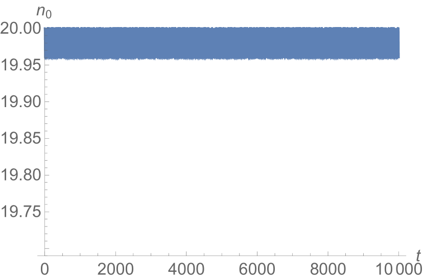
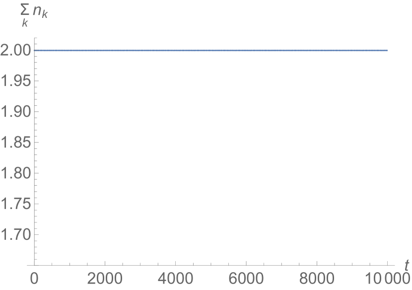
(a) $C_{\text{m}}=0$.

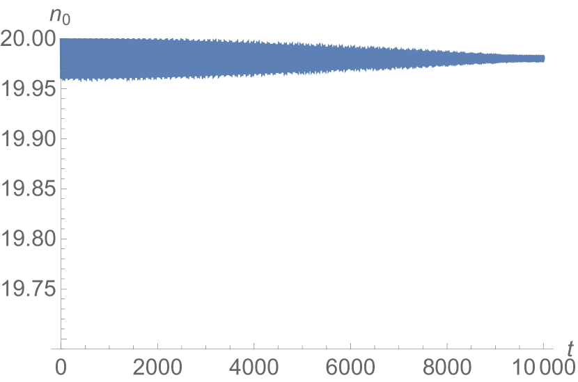
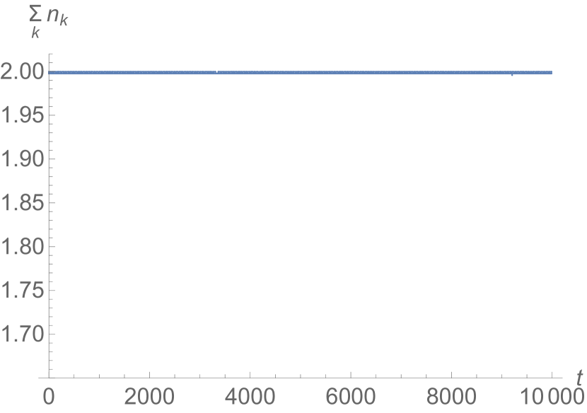
(b) $C_{\text{m}}=0.1$.

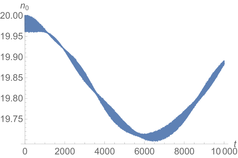
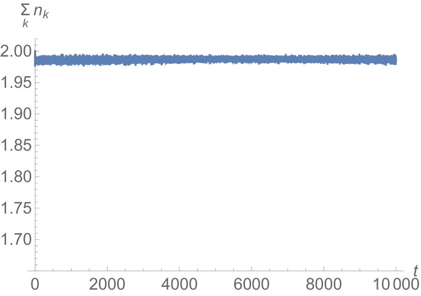
(c) $C_{\text{m}}=0.30055$.

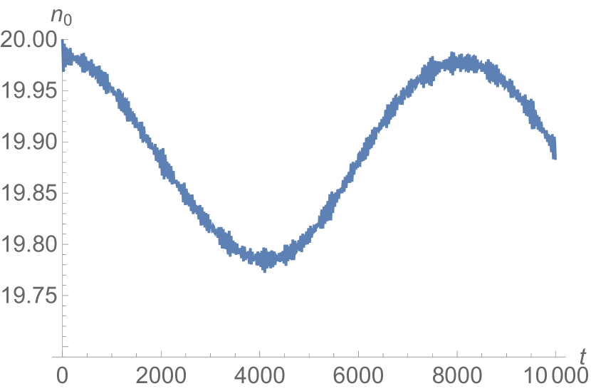
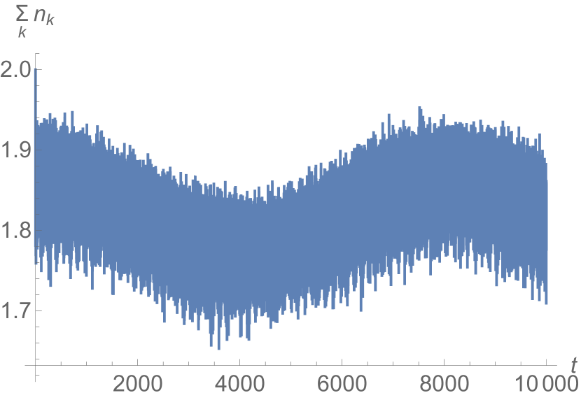
(d) $C_{\text{m}}=1.239$.

Figure 2: Time evolution of the initial state (35) for different values of $C_{\text{m}}$. Oscillations on a timescale of order $1$ cannot be resolved graphically any more since we show very long timescales. $n_{0}$ is the expectation value of the occupation of the mode $\hat{a}_{0}$ and $\sum_{k}n_{k}$ that of the total occupation in the first critical sector. Time is plotted in units of $\epsilon_{0}^{-1}\hbar$.

The time evolution of the initial state (35) for different values of $C_{\text{m}}$ is displayed in Fig. 2, where we show the expectation value $n_{0}$ of the occupation number of the $\hat{n}_{0}$-mode as well as the expectation value of the total occupation of the first critical sector $\sum_{k=1}^{K}\hat{n}_{k}$. For $C_{\text{m}}=0$ (see Fig. 2(a)), we can replace $\sum_{k=1}^{K}\hat{n}_{k}\rightarrow N_{m}$ and $\sum_{k^{\prime}=1}^{K^{\prime}}\hat{n}^{\prime}_{k^{\prime}}\rightarrow 0$ and the system has the analytic solution (9). We observe that the critical sector does not move and the amplitude of oscillations of $\hat{n}_{0}$ is strongly suppressed. This is the effect of memory burden [1] discussed before in section II.2.

For many nonzero values of $C_{\text{m}}$, the system behaves similarly (see Fig. 2(b)). Although the time evolution of the system becomes more involved, the amplitude of oscillations of $n_{0}$ is still small and the critical sectors remains effectively frozen.

However, there are certain values of $C_{\text{m}}$ for which the system behaves qualitatively differently and the amplitude of oscillations of $n_{0}$ increases distinctly, albeit on a significantly longer timescale (see Figs. 2(c), 2(d)). As expected, this behavior is accompanied by a change of the occupation numbers in the critical sector. This can either happen via an instantaneous jump (as in Fig. 2(c)) or via oscillations that are synchronous with $n_{0}$ (as in Fig. 2(d)). Although the second scenario is more intuitive than the first one, both are in line with our statement that $n_{0}$ can only change significantly if also rewriting in the critical sector takes place. Moreover, we note that the occupation transfer and thus the rewriting of information is not complete. We expect that complete rewriting into the second sector of memory modes can be achieved only after including further sectors, to which the $\hat{a}^{\prime}_{k^{\prime}}$-modes can transfer occupation number.

We shall call the values of $C_{\text{m}}$ for which partial rewriting takes place rewriting values. For the present values of the remaining parameters (III), such values are rare. In order to illustrate this point, we plot the maximal amplitude of oscillations as a function of $C_{\text{m}}$ in Fig. 3(a). We remark, however, that for other parameter choices, we have observed much more abundant rewriting values.

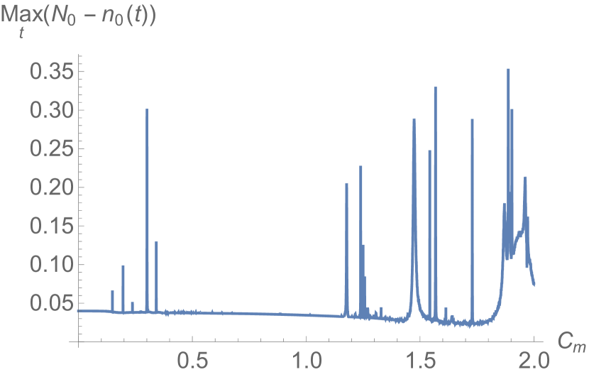
(a) $p=1\,,~{}C_{0}=0.01$

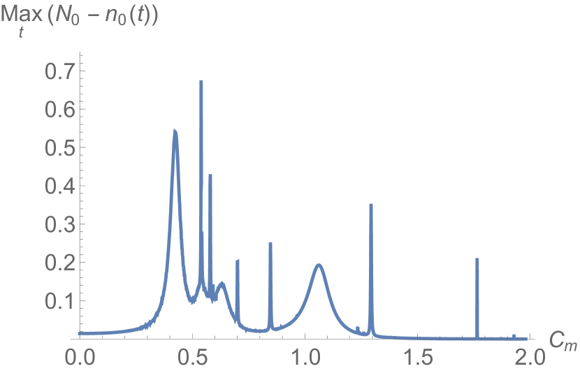
(b) $p=2\,,~{}C_{0}=0.0003$

Figure 3: Maximal amplitude of the expectation value of $\hat{n}_{0}$ for different values of $C_{\text{m}}$ (with initial state (35)).

Finally, we also study how the system behaves when we choose $p=2$ (see Eq. (12)), i.e., we replace $1-\hat{n}_{0}/N_{c}\rightarrow(1-\hat{n}_{0}/N_{c})^{2}$ and $1-\hat{n}_{0}/(N_{c}-\Delta N_{c})\rightarrow(1-\hat{n}_{0}/(N_{c}-\Delta N_{c}))^{2}$. As is evident from Eq. (14), this reduces the memory burden by a factor of approximately $0.03$ (we used that $N_{c}-n_{0}$ can get as large as $0.3$ in the case $p=1$; see Fig. 3(a)). In order to keep the amplitude of oscillation in the absence of rewriting (see Eq. (9)) on the same order of magnitude as for $p=1$, we reduce $C_{0}$ by the same factor, i.e., set $C_{0}=0.0003$. Apart from this change, we use the values displayed in Eq. (III). As in the case $p=1$, we time evolve the system for different values of $C_{\text{m}}$. The resulting maximal amplitude as a function of $C_{\text{m}}$ in displayed Fig. 3(b). Qualitatively, we observe the same behavior as for $p=1$.

III.2 Dependence on System Size

After having seen that rewriting does indeed take place, we now wish to answer the question how this changes as the size of the system increases. In order to answer it, we investigate how the rewriting values of $C_{m}$ change as we vary the parameters of the Hamiltonian (34). Moreover, it is possible to determine a rate $\Gamma$ of rewriting as the ratio of the maximal amplitude of $n_{0}$ and the timescale on which this maximal value is attained. If we map our system on a decay process, as we have e.g., done in section II.5, we can identify this rate with the decay rate. We shall also study how the rate $\Gamma$ changes as we vary the parameters. In the following, we restrict ourselves to the case $p=1$. All numerical data that lead to the results shown subsequently are publicly available in the companion Zenodo record [26].

As presented in the appendix, the observed scalings for $C_{m}$ and $\Gamma$ are as follows:

• The initial occupation number $N_{c}$ of $\hat{n}_{0}$ (which is also the critical occupation at which the first memory sector is gapless):

  $$C_{\text{m}}\sim N_{c}^{-1}\,,\qquad\Gamma\sim N_{c}^{-1}$$ (37)

• The free gap $\epsilon_{m}$ of the memory modes:

  $$C_{\text{m}}\sim\epsilon_{m}^{1}\,,\qquad\Gamma\sim\epsilon_{m}^{0}\ \text{(independent)}$$ (38)

• The coupling $C_{0}$ of $\hat{a}_{0}$ and $\hat{b}_{0}$:

  $$C_{\text{m}}\sim C_{0}^{0}\ \text{(independent)}\,,\qquad\Gamma\sim C_{0}^{1.4}$$ (39)

• The difference $\Delta N_{c}$ between the critical occupations of $\hat{a}_{0}$ making either of the two memory sectors gapless:

  $$C_{\text{m}}\sim(\Delta N_{c}/N_{c})^{0.2}\,,\qquad\Gamma\sim(1-\Delta N_{c}/N_{c})$$ (40)

With regard to the $K$ and $K^{\prime}$, we can unfortunately only study three values due to numerical limitations, namely $K=K^{\prime}=4,6,8$. The results are displayed in Fig. 4, where we take $N_{m}=K/2$. Since we cannot make a precise statement about the dependence on $K$, we will parameterize it as

$$C_{\text{m}}\sim K^{\beta_{C}}\,,\qquad\Gamma\sim K^{\beta_{\Gamma}}\,.$$ (41)

Still, we can try to constrain rewriting, i.e., give a lower bound on $C_{m}$ and an upper bound on $\Gamma$. To this end, we calculate the mean value of $C_{m}$ for the 11 data points at $K=6$. In order to obtain a maximally conservative bound, we moreover choose among the results for $K=8$ the 11 data points with the lowest values of $C_{m}$ and compute their mean. Performing a fit with the two resulting mean values, we get

$$\beta_{C}\gtrsim-0.7\,.$$ (42)

We have not included the value at $K=4$ since doing so would increase $\beta_{C}$. For $\Gamma$, we compute the mean value for the 11 data points at $K=6$. At $K=8$, we choose the 11 data points with the highest rates and calculate their mean. Fitting the resulting two means together with the rate of the single rewriting value at $K=4$, we arrive at

$$\beta_{\Gamma}\lesssim-0.7\,.$$ (43)

In this case, we have not excluded the value at $K=4$ because this would decrease $\beta_{\Gamma}$. Even though we have tried to be conservative in our estimates, we must stress that we have far too little data to make any reliable statement. Thus, the true values of $\beta_{C}$ and $\beta_{\Gamma}$ might not respect the bounds (42) and (43).

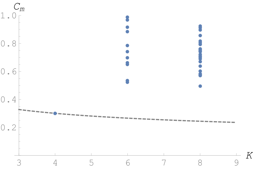
(a) Rewriting values of $C_{\text{m}}$

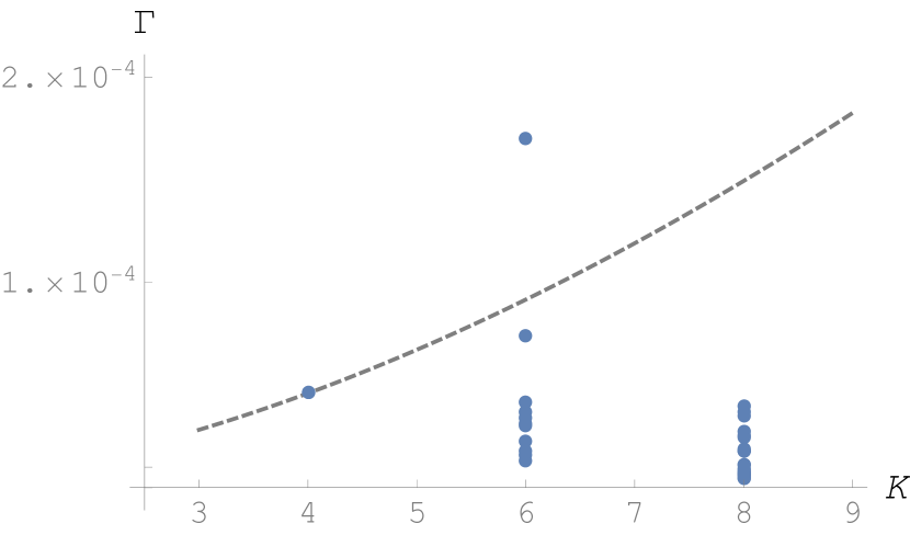
(b) Rates $\Gamma$ at those rewriting values

Figure 4: Available data (blue dots) for the rewriting values of $C_{m}$ and the rates $\Gamma$ as function of $K=K^{\prime}$, where we take $N_{m}=K/2$. The dashed curves are the constraints (57) and (58), that apply to a black hole. We see clear indications that for large black holes, rewriting is not fast enough to reproduce the semiclassical rate of evaporation.

In summary, we observe that the rate $\Gamma$ decreases as the system size increases, i.e., as $N_{c}$ or $K$ gets bigger (see Eqs. (37) and (43)). Whereas $C_{0}$ can vary independently in a generic system, Eq. (33) shows that it decreases with system size in the black hole case. Therefore, the observed scaling (39) reinforces the tendency of lowering $\Gamma$. Thus, we see clear indications that rewriting becomes more difficult for larger systems.

III.3 Understanding Our Results

In this chapter, we shall provide some analytic understanding of our findings. For simplicity we take $K=K^{\prime}$, and assume each memory set to be diagonal with the equal gaps. Thus, we take $\tilde{C}_{k,l}=\tilde{C}_{k^{\prime},l^{\prime}}=0$ and $\epsilon_{k}$ and $\epsilon_{k^{\prime}}$ to be universal, i.e., for all $k,k^{\prime}$, $\epsilon_{k}=\epsilon_{k^{\prime}}=\sqrt{N_{c}}\epsilon_{0}$. Then, without any loss of generality, the matrix $C_{k,k^{\prime}}$ can be set diagonal since we can always achieve this by an unitary transformation. The Hamiltonian (16) then becomes,

$$\hat{H} =\epsilon_{0}\hat{n}_{0}+\epsilon_{0}\hat{m}_{0}+C_{0}\left(\hat{a}_{0}^{\dagger}\hat{b}_{0}+\hat{b}_{0}^{\dagger}\hat{a}_{0}\right)$$

$$+{\mathcal{E}}\sum_{k}\hat{n}_{k}+{\mathcal{E}}^{\prime}\sum_{k}\hat{n}_{k}^{\prime}$$

$$+\sum_{k}C_{k,k}\left(\hat{a}_{k}^{\dagger}\hat{a}^{\prime}_{k}+\text{h.c.}\right)\,,$$

where

$${\mathcal{E}}\equiv\sqrt{N_{c}}\left(1-\frac{\hat{n}_{0}}{N_{c}}\right)\epsilon_{0}\,,$$ (45)

and

$${\mathcal{E}}^{{}^{\prime}}\equiv\sqrt{N_{c}}\left(1-\frac{\hat{n}_{0}}{N_{c}-\Delta N_{c}}\right)\epsilon_{0}\,.$$ (46)

Now, in the initial state (17), $n_{0}=N_{c}$ and we have

$${\mathcal{E}}=0\,,~{}{\mathcal{E}}^{{}^{\prime}}\simeq-\frac{\Delta N_{c}}{\sqrt{N_{c}}}\epsilon_{0}<0\,.$$ (47)

Since the second gap is negative, there exist states with much lower energy than the initial one (17). In particular, such is the state

$$\ket{\text{low}}=\ket{\underbrace{N_{c}}_{n_{0}},\underbrace{0}_{m_{0}},0,\ldots 0,\underbrace{n_{1}}_{n^{\prime}_{1}},\ldots,\underbrace{n_{K}}_{n^{\prime}_{K}}}\,.$$ (48)

This is the state obtained from (17) by exchanging the occupation numbers of the two memory sectors, $n_{k}\leftarrow\rightarrow n_{k}^{\prime}$, without touching $n_{0}$ and $m_{0}$. This state has a macroscopically large negative energy difference with respect to (17). Expressing this energy difference in terms of the memory burden, which in this case implies $\epsilon_{0}\sum_{k}n_{k}=-\mu\sqrt{N_{c}}$, we have,

$$\bra{\text{low}}\hat{H}\ket{\text{low}}-\bra{\text{in}}\hat{H}\ket{\text{in}}={\mathcal{E}}^{\prime}\sum_{k}n_{k}\sim\Delta N_{c}\mu\,.$$ (49)

Since $\mu<0$, the energy of (48) is much lower than the energy of the initial state (17).

The above makes it clear that we should be able to take intermediate deformations of the initial state (17) in which the exchange of the occupation number between the sets $n_{k}$ and $n_{k}^{\prime}$ is balanced by the exchange between $n_{0}$ and $m_{0}$ in such a way that the obtained state is nearly degenerate with the initial one.

It therefore looks plausible that the system can use such a path for overcoming the memory burden. This was our original expectation as well as the proposal in [1, 2]. Yet, this is not what we are finding.

Instead we discover that the system cannot evolve efficiently. The reason for this is the following. The maintenance of the zero energy balance along the current trajectory requires a synchronous evolution of the two sets of degrees of freedom, $a_{0},b_{0}$ and $a_{k},a_{k}^{\prime}$, respectively. These sets have to produce opposite contributions into the energy that cancel each other. Basically, one set has to “climb up” the energy stairs while the other is coming down.

However, each evolution has a highly suppressed amplitude due to the huge gap differences among the proper modes. This breaks the process.

In order to see this, let us consider the time evolution near the initial state (17). This time evolution can be described as set of coupled $2\times 2$ problems, with the following Hamiltonians,

$$\hat{H}=\sum_{k}\bordermatrix{&\hat{a}_{k}&\hat{a}_{k}^{{}^{\prime}}\cr\hat{a}_{k}^{\dagger}&0&C_{k,k}\cr\hat{a}_{k}^{{}^{\prime}\dagger}&C_{k,k}&{\mathcal{E}}^{\prime}\cr}+\bordermatrix{&\hat{a}_{0}&\hat{b}_{0}\cr\hat{a}_{0}^{\dagger}&\epsilon_{0}+\mu&C_{0}\cr\hat{b}_{0}^{\dagger}&C_{0}&\epsilon_{0}\cr}\,.$$ (50)

The systems are coupled because ${\mathcal{E}}^{\prime}$ is a function of $n_{0}$, whereas $\mu$ is a function of $\sum_{k}n_{k}$.

The qualitative behavior can be understood by solving the system iteratively, i.e., in the zeroth order approximation, we evolve the system by treating ${\mathcal{E}}^{\prime}$ and $\mu$ as constants. We then evolve them in the first order by taking into account the variations of the occupation numbers obtained in the zeroth order.

It is immediately clear that the amplitudes of both transitions are highly suppressed because of the huge eigenvalue-splittings in the corresponding $2\times 2$ matrices. Namely, we have

$$\delta n_{0}\sim-N_{c}\frac{C_{0}^{2}}{\mu^{2}}\,~{}~{}{\rm and}~{}~{}\delta n_{k}\sim-\frac{C_{k,k}^{2}}{{\mathcal{E}}^{{}^{\prime}2}}\,.$$ (51)

The resulting variations of ${\mathcal{E}}^{{}^{\prime}}$ and $\mu$ are so small that they cannot affect the picture in the next iteration. For example, we can assume $K=N_{c}=\sum_{k}n_{k}$ and take into account the bound $C_{0}\lesssim\epsilon_{0}/\sqrt{N_{c}}$, which arises in the black hole case (see Eq. (33)), as well as condition (22),

$$\frac{C_{k,k}^{2}}{{\mathcal{E}}^{{}^{\prime}}}\lesssim\frac{\epsilon_{0}}{\sqrt{N_{c}}}\,.$$ (52)

Then we get

$$\frac{\delta\mu}{\mu}\lesssim\frac{\epsilon_{0}}{\sqrt{N_{c}}{\mathcal{E}}^{{}^{\prime}}}\,~{}~{}{\rm and}~{}~{}\frac{\delta{\mathcal{E}}^{{}^{\prime}}}{{\mathcal{E}}^{{}^{\prime}}}\sim\frac{1}{\Delta N_{c}N_{c}}\,.$$ (53)

Finally, we take into account that there is a lower bound on $|{\mathcal{E}}^{{}^{\prime}}|$ (Eq. (20) or (21)). Even the mildest bound (20) suffices to conclude that the iteration series rapidly converge towards the result that the system is essentially trapped in the initial state. Moreover, we note that (52) acquires an additional factor $1/\sqrt{N_{c}}$ if the effective gaps do not come with both positive and negative signs (see footnote 1).

III.4 Application to Black Hole

Now we adapt the parameter choice (II.5) that corresponds to the case of a black hole. In this situation, only the couplings $C_{0}$ and $C_{\text{m}}$ as well as $\Delta N_{c}$ remain independent of $S$. However, $C_{0}$ is related to $S$ through the bound (33), which is specific to black holes. Likewise, Eq. (20) leads to a bound on $\Delta N_{c}$, namely

$$\Delta N_{c}\gg 1\,.$$ (54)

Using the observed scalings stated in Eqs. (37)-(39), we get for $C_{\text{m}}$

$$C_{\text{m}}\sim S^{-0.5+\beta_{C}}(\Delta N_{c}/S)^{0.2}\gtrsim S^{-0.7+\beta_{C}}\,,$$ (55)

as well as

$$\Gamma\sim S^{-1.7+\beta_{\Gamma}}\,.$$ (56)

Eq. (55) shows that in order to satisfy the bound (30) on the $S$-dependence of $C_{m}$, the scaling of $C_{m}$ with $K$ would be constrained as

$$\beta_{C}\lesssim-0.3\,.$$ (57)

Analogously, it follows from Eq. (56) that the requirement of reproducing the semiclassical value of the rate, $\Gamma\sim 1$, leads to

$$\beta_{\Gamma}\gtrsim 1.7\,.$$ (58)

Now we would like to investigate the compatibility of the numerical results for $K$-variation with the bounds in Eqs. (57) and (58). Firstly, we compare the actual results for $K=6,8$ with the expectation for $K=6,8$ based on the result for $K=4$ and a scaling saturating the bounds Eqs. (57) and (58). The resulting functions are plotted in Fig. 4. We observe that although many more rewriting values exist at higher $K$, none of them satisfies both the constraints (57) and (58).

As a different method of analysis, we can compare the bounds (57) and (58) with the estimates (42) and (43). We observe that $\beta_{C}$ might be small enough, but $\beta_{\Gamma}$ is vastly different. These are clear indications that for large black holes rewriting of information from one memory sector to another one cannot be efficient enough to reproduce the semiclassical rate of particle creation, $\Gamma\sim 1$. As far as we can numerically access the system, we therefore conclude that even if rewriting takes place, the semiclassical description breaks down as soon as memory burden sets in.

We expect the semiclassical approximation to be valid as long as a newly created black hole has not lost a sizable fraction of its mass. In the absence of sufficiently fast rewriting, the model (34), which we have studied here, does not fulfill this requirement because it would lead to an immediate deviation from the semiclassical rate of particle production. Therefore, an effective description of black hole evolution must realize an appropriate delay of the onset of the memory burden effect. As reviewed in II.2, the model (12) (with a parameter choice $p\gg 1$) achieves such a delay. It can do so at most until the master mode has lost on the order of half of its initial occupation, and, correspondingly, until the black hole has lost on the order of half of its mass.

We can give a quantitative estimate of how strong the slowdown is at that point, assuming that the rewriting rate after the onset of backreaction in the system (12) (with a parameter value $p\gg 1$ and including the coupling to another set of memory modes) behaves analogously to the system investigated here. To this end, we first note that $C_{0}\sim 1/S$ is required in order to reproduce the semiclassical rate of Hawking evaporation, $\Gamma\sim 1$, during the initial evolution before the onset of memory burden. Consequently, Eq. (56) gets modified:

$$\Gamma\sim S^{-2.4+\beta_{\Gamma}}\,.$$ (59)

As explained, we cannot determine $\beta_{\Gamma}$ due to numerical limitations. Still, we can try to give a bound on it. Since we clearly see no indications that the rates increase with $K$ (see Eq. (43)), we can conservatively estimate that $\beta_{\Gamma}<0$. Then we obtain

$$\Gamma\lesssim\frac{1}{S^{2}}\,.$$ (60)

Thus, evaporation has to slow down drastically at the latest after the black hole lost on the order of half of its initial mass.

III.5 Regime After Metamorphosis

In the following, we will discuss scenarios of BH evolution beyond half-decay that are consistent with the above finding. In the standard semiclassical treatment, the evaporation process of a black hole is taken to be self-similar, i.e., it is assumed to be well described simply by a time-dependent mass $M(t)$ which in each moment of time determines the Schwarzschild radius and the temperature as $r_{g}=2G_{N}M(t)$ and $T=(8\pi G_{N}M(t))^{-1}$, respectively. This leads to the picture of a thermal emission spectrum shifting with the growing temperature as the evaporation proceeds. Thus, the assumption is that a classical black hole with each quantum emission evolves into a classical black hole of a lower mass. This picture is widely accepted, despite the fact that there exist no self-consistent semi-classical calculation giving such a time evolution.

It is quite contrary [27]: This picture has a built-in measure of its validity since the above equation, together with $\dot{M}\sim r_{g}^{-2}$, leads to $\dot{T}/T^{2}\sim 1/S$. This quantity sets the lower bound on the deviation from thermality. It vanishes only in strict semi-classical limit $G_{N}\rightarrow 0,~{}M\rightarrow\infty,~{}r_{g}=\text{finite}$. It is important to note that in this limit $S\rightarrow\infty$. Therefore, the standard Hawking result is exact. However, for finite mass black holes and non-zero $G_{N}$, the deviations from thermal spectrum are set by $1/S$.

Already this fact tells us that it is unjustified to use the self-similar approximation over timescales comparable with black hole half-decay, $\tau\sim Sr_{g}$. Indeed, without knowing the microscopic quantum theory, one can never be sure that the semi-classical approximation is not invalidated due to a build-up of quantum back-reaction over the span of many emissions.

As microscopic theory tells us [3, 15, 16, 17], this is exactly what is happening: At the latest by the time a black hole loses of order of half of its mass, the back-reaction is so strong that the semiclassical treatment can no longer be used. In particular, the remaining black hole state is fully entangled after losing on the order of half of its constituents.

The present study reveals a new microscopic meaning of the quantum back reaction. Namely, being states of maximal memory capacity, the black holes are expected to share the universal property of memory burden. Due to this phenomenon, the black hole evaporation rate must change drastically after losing half of its mass. What happens beyond this point can only be a subject to a guess work. However, given the tendency that the memory burden resist the quantum evaporation, the two possible outcomes are: 1) A partial stabilization by slowing down the evaporation; 2) Classical disintegration into some highly non-linear gravitational waves. The second option becomes possible because after the breakdown of the description in terms of a classical black hole, we cannot exclude any more that the system exhibits a classical instability. Obviously, there could be a combination of the two options, where a prolonged period of slow evaporation transits into a classical instability. In the following, we shall focus on the first option as being the most interesting for the dark matter studies.

Thus, motivated from our analysis of the prototype model, we shall adopt that the increased lifetime due to the slowdown is

$$\tilde{\tau}\gtrsim r_{g}S^{1+k}\,,$$ (61)

where $k$ indicates the power of additional entropy suppression of the decay rate as compared to the semiclassical rate, $\Gamma\sim r_{g}^{-1}$. Although the spectrum is no longer thermal, we shall assume that the mean wavelength of quanta emitted during this stage is still on the order of the initial Schwarzschild radius $\sim r_{g}$, as long as the mass is still on the order of the initial mass. We must stress, however, that we cannot exclude that the black hole starts emitting much harder quanta after memory burden has set in. In particular, as the gap increases, the memory modes become easier-convertible into their free counterparts. This conversion is likely a part of the mechanism by which the information starts getting released after the black hole’s half decay.

IV Role of Number Non-Conservation

In our previous analysis we have explained the essence of the memory burden phenomenon and studied its manifestations on prototype systems numerically. In these prototype systems we have limited ourselves to particle number conserving interactions. One may wonder how important the role of particle number conservation is. In this section we wish to explain that it is not.

In order to understand this, let us first briefly recount the essence of the phenomenon which is the following. A set of memory modes, which we have denoted by $\hat{a}_{k}$-s, becomes gapless when the occupation number of the master mode, $\hat{a}_{0}$, reaches a certain critical value $n_{0}=N_{c}$. This allows to populate the memory modes – and therefore store the memory patterns of the form (5) – without any expense in energy. This memory pattern creates a backreaction on a master mode by generating a high energy gap for it. We call this gap a memory burden and denote it by the symbol $\mu$.

The net effect of this backreaction is that it resists to any departure of the master mode away from criticality. This is because the information pattern stored in the memory modes (5) becomes costly in energy as soon as the the master mode moves away from the critical value. The change of energy, resulting from the variation $\Delta n_{0}$ of the master mode, is:

$$\Delta E_{\rm pattern}=\mu\,\Delta n_{0}\,.$$ (62)

As a result, a force is created that prevents the occupation number of the master mode from changing.

In order to allow for such a change, the system must get rid of the memory burden $\mu$ by somehow decreasing the occupation number of the memory modes. The pattern stored in these modes then must be rewritten in some other set of modes which we have denoted by $\hat{a}^{\prime}_{k^{\prime}}$. Our simulations indicate that for the reasonable choice of the parameter values, in particular motivated by scalings in black hole analogs, the rewriting process is not nearly efficient for avoiding the memory burden, i.e., the process of offloading the memory modes from the $\hat{a}_{k}$-sector into $\hat{a}^{\prime}_{k^{\prime}}$ cannot be synchronized with the decay of the $\hat{a}_{0}$-mode.

So far, in our examples, both processes were modeled by interactions that conserve the total number of particles, i.e., the destruction of an $\hat{a}_{k}$-mode was accompanied by a creation of a particle from another sector. Likewise, the destruction of an excitation of the master mode $\hat{a}_{0}$ was accompanied by a creation of a $\hat{b}_{0}$-quantum.

Our analysis showed that the memory burden effect was so strong that it killed the decay process before the extra sectors ($\hat{a}^{\prime}_{k^{\prime}},\hat{b}_{0}$) had any chance to be significantly populated. Correspondingly, the inverse transition processes played no role in the time-evolution of the system.

In these circumstances, it is clear that the role of particle number conservation is insignificant. Namely, the transitions generated by the particle number non-conserving interactions of similar strengths would be equally powerless against the memory burden effect. Let us estimate this explicitly.

IV.1 Number non-conserving decay of the master mode

We shall first consider the effect of number non-conserving decays of the master mode. We take the fixed memory burden $\mu$ and replace the number conserving mixing between $\hat{a}_{0}$- and $\hat{b}_{0}$-modes in (7) by the following number-non-conserving one,

$$\hat{H}=(\epsilon_{0}+\mu)\hat{a}^{\dagger}_{0}\hat{a}_{0}\,+\epsilon_{0}\hat{b}^{\dagger}_{0}\hat{b}_{0}+C_{0}(\hat{a}_{0}\hat{b}_{0}+\hat{a}_{0}^{\dagger}\hat{b}_{0}^{\dagger})\,,$$ (63)

where we have taken the parameter $C_{0}$ to be real and of the same strength as in the number-conserving version (7). This strength, $C_{0}\sim\epsilon_{0}/N_{c}$, is dictated by the requirement that for $\mu=0$ the half-decay time of the $\hat{a}_{0}$-mode is $t\sim N_{c}/\epsilon_{0}$ as it is clear from (9). This choice imitates, at the level of our toy model, the scaling of the black hole half-decay time in units of the energy of the Hawking quanta.

The Hamiltonian (63) is diagonalized by the following Bogoliubov transformation:

$$\hat{a}_{0}=u\hat{\alpha}-v\hat{\beta}^{\dagger}\,,\qquad\hat{b}_{0}=u\hat{\beta}-v\hat{\alpha}^{\dagger}\,,$$ (64)

where $\hat{\alpha}$ and $\hat{\beta}$ are the eigenmodes and

$$v^{2} =\frac{1}{2}\left(\frac{1}{\sqrt{1-\frac{4C_{0}^{2}}{(2\epsilon_{0}+\mu)^{2}}}}-1\right),$$ (65)

$$u^{2} =\frac{1}{2}\left(\frac{1}{\sqrt{1-\frac{4C_{0}^{2}}{(2\epsilon_{0}+\mu)^{2}}}}+1\right)\,.$$ (66)

For the full memory burden, we have $\mu\sim-\epsilon_{0}\sqrt{N_{c}}$. Taking into account that $C_{0}\sim\epsilon_{0}/N_{c}$, Eq. (65) gives,

$$v^{2}\simeq\frac{C_{0}^{2}}{\mu^{2}}\sim\frac{1}{N_{c}^{3}}\,,~{}~{}~{}u^{2}=1+{\mathcal{O}}(1/N_{c}^{3})\,,$$ (67)

Thus, the depletion coefficient $v^{2}$ is minuscule due to an extra $1/N_{c}$-suppression by the memory burden factor $\frac{\epsilon_{0}}{\mu}$. We note that the amplitude in the case of a number conserving mixing is suppressed by the same factor $C_{0}^{2}/\mu^{2}$ (see Eq. (9)).

The similarity between the two cases in the present situation, in which the occupation number of the $\hat{b}_{0}$-mode never becomes high whereas the occupation number of $\hat{a}_{0}$ is macroscopic, can also be understood in the Bogoliubov approximation, in which we replace number operators of the $\hat{a}_{0}$-mode by $c$-numbers, $\hat{a}_{0}=\sqrt{N_{c}}\,,~{}\hat{a}_{0}^{\dagger}=\sqrt{N_{c}}$. After disregarding terms smaller than $1/\sqrt{N_{c}}$, the number non-conserving Hamiltonian (63) becomes:

$$\hat{H}=\epsilon_{0}\hat{b}^{\dagger}_{0}\hat{b}_{0}+C_{0}\sqrt{N_{c}}(\hat{b}_{0}^{\dagger}+\hat{b}_{0})\,.$$ (68)

This is easily brought to a diagonal form by a canonical transformation

$$\hat{b}_{0}=\hat{\beta}-C_{0}\sqrt{N_{c}}/\epsilon_{0}\,,$$ (69)

which shows that the occupation number of the $\hat{b}_{0}$-mode in the $\beta$-vacuum is,

$$\langle\hat{b}_{0}^{\dagger}\hat{b}_{0}\rangle=\frac{C_{0}^{2}N_{c}}{\epsilon_{0}^{2}}\,.$$ (70)

Thus, depletion is still suppressed by $C_{0}$. The above argument is another way of understanding why – as long as the occupation number of $\hat{b}_{0}$ is small and therefore the inverses processes are not effective – the number conserving versus number non-conserving nature of the mixing is not important. Thus, it is clear that number non-conservation does not allow to circumnavigate the memory burden effect.

Further notice that the relative effect of possible decays of the $\hat{a}_{0}$-mode into several $\hat{b}_{0}$-quanta is negligible. In the interaction vertex each extra $\hat{b}_{0}$ brings an additional factor of $1/\sqrt{N_{c}}$. So, the coefficient of the term $\hat{a}_{0}\hat{b}_{0}^{l}$ scales as $\epsilon_{0}/N_{c}^{l/2}$.

IV.2 Number non-conserving decay of memory modes

Let us now ask whether a number non-conserving decay of the memory modes could ease the memory burden effect more rapidly as compared to a number conserving one. In order to answer this question, we shall allow for a depletion of the memory modes due to a number non-conserving mixing with another sector.

Before doing so we wish to clarify the following point. Notice that for odd values of $p$ the effective gap of the second layer of the memory modes becomes negative. For a number conserving Hamiltonian, this makes no difference in the memory burden effect. Therefore we can use the simplest version of $p=1$ (see (13)) in our discussions.

However, once we allow for number non-conservation among memory modes, the negative gap can lead to “tachyonic” type instabilities that can populate the memory modes by creating them out of the vacuum. This increase of the occupation number has nothing to do with easing a memory burden on the first sector but rather is a manifestation of instability. Still, such instability blurs the question that we are after. So we shall assume that the gap is always positive. This assumption is equivalent to the statement that there are no intrinsic tachyonic instabilities in the initial state of the system. This imposes a constraint on the structure of the Hamiltonian, which we will take into account below.

Let us consider the following Hamiltonian that mixes the memory modes,

$$\hat{H} ={\mathcal{E}}_{k}\hat{n}_{k}+{\mathcal{E}}_{k^{\prime}}\hat{n}^{\prime}_{k^{\prime}}+$$

$$+C_{k,k^{\prime}}\left(\hat{a}_{k}\hat{a}^{\prime}_{k^{\prime}}+\text{h.c.}\right)\,.$$ (71)

For simplicity of illustration, we paired-up the modes from the two sets, effectively reducing the evolution to a $2\times 2$ problem. Making a more complicated mixing matrix does not change the qualitative picture.

The quantities ${\mathcal{E}}_{k}$ and ${\mathcal{E}}_{k^{\prime}}$ are effective gaps that are functions of $n_{0}$. The only requirement that we need to specify is that they alternatively reach zeros for two critical values $n_{0}=N_{c}$ and $n_{0}=N_{c}-\Delta N_{c}$ respectively, and are semi-positive definite everywhere in between. Moreover, at the critical points the level splitting is macroscopic:

$${\mathcal{E}}_{k}=0\,,{\mathcal{E}}_{k^{\prime}}\gg\epsilon_{0}, \qquad\text{for}~{}n_{0}=N_{c},$$

$${\mathcal{E}}_{k^{\prime}}=0\,,{\mathcal{E}}_{k}\gg\epsilon_{0}, \qquad\text{for}~{}n_{0}=N_{c}-\Delta N_{c}.$$ (72)

For example, we can choose

$${\mathcal{E}}_{k}\equiv\left(1-\frac{\hat{n}_{0}}{N_{c}}\right)\epsilon_{k}\,,$$ (73)

as before, and for ${\mathcal{E}}_{k^{\prime}}$ assume one of many possible shapes, e.g.,

$${\mathcal{E}}_{k^{\prime}}\equiv\left(1-\frac{\hat{n}_{0}}{N_{c}-\Delta N_{c}}\right)^{2}\epsilon_{k^{\prime}}\,,$$ (74)

or

$${\mathcal{E}}_{k^{\prime}}\equiv\left(\frac{\hat{n}_{0}}{N_{c}-\Delta N_{c}}-1\right)\epsilon_{k^{\prime}}\,,~{}$$ (75)

and so on. Finally, as in the number conserving case, to which we wish to compare the evolution of the present system, the parameter $C_{k,k^{\prime}}$ cannot be too big since otherwise the gaplessness of $\hat{a}_{k}$-modes at the critical point $n_{0}=N_{c}$ would be destroyed. This leads to the condition (52).

Now, let us recall that the reason why the depletion of the gapless memory modes in the particle number-conserving case (16) was not efficient, is:

• Relatively large level-splitting: $\Delta{\mathcal{E}}={\mathcal{E}}_{k^{\prime}}-{\mathcal{E}}_{k}$

• Suppressed mixing coefficient $C_{k,k^{\prime}}$.

As long as these conditions are maintained, allowing the particle number non-conservation in the mixing term does not improve the situation. Indeed, we diagonalize the Hamiltonian via the Bogoliubov transformation,

$$\hat{a}_{k}=u\hat{\alpha}_{k}-v\hat{\beta}_{k^{\prime}}^{\dagger}\,,\qquad\hat{a}_{k^{\prime}}^{\prime}=u\hat{\beta}_{k^{\prime}}-v\hat{\alpha}_{k}^{\dagger}\,,$$ (76)

where

$$u^{2}=1+v^{2}\,,~{}v^{2}=\frac{1}{2}\left(\frac{1}{\sqrt{1-\frac{4C_{k,k^{\prime}}^{2}}{({\mathcal{E}}_{k}+\,{\mathcal{E}}_{k^{\prime}})^{2}}}}-1\right)\,.$$ (77)

Next, taking into account Eqs. (52) and (IV.2), we have near $n_{0}=N_{c}$

$$v^{2}\sim\frac{C_{k,k^{\prime}}^{2}}{({\mathcal{E}}_{k^{\prime}})^{2}}\ll\frac{\epsilon_{0}}{\sqrt{N}{\mathcal{E}}_{k^{\prime}}}\,,\qquad\,u^{2}\simeq 1\,,$$ (78)

which gives a highly suppressed rate of offloading the memory pattern. This rate is negligible and of no help for liberating the master mode $\hat{a}_{0}$ from the memory burden effect on any reasonable timescale.

Finally, as in the previous example, the higher order operators, e.g., $\hat{a}_{k}\hat{a}_{k_{1}^{\prime}}^{\prime}\cdots\hat{a}_{k_{l}^{\prime}}^{\prime}$, (whether number conserving or not) cannot improve the decay rate due to the extra suppression by powers of $1/N_{c}$.

IV.3 Summing up

We are now ready to summarize the discussion about the role of number (non-)conservation in easing the memory burden. The memory burden phenomenon is a relative effect that amounts to a delay of the time evolution of the system due to a backreaction of the memory pattern. In order to measure its effect, we must do so by comparing the time evolution of the same system with and without the initial memory pattern.

Motivated by the black hole analogy, we have normalized (in units of an elementary gap $\epsilon_{0}$) the half-decay time of the system with $\mu=0$ (an empty memory pattern) to $N_{c}$. This timescale fixes the strengths of the leading operators that can reduce the number of the master mode.

We then study the system, with maximal memory burden $\mu$ (fully loaded memory pattern), assuming the strict conservation of the occupation number of the memory modes $\hat{a}_{k}$. In this case, we see that the memory burden stops the leakage of the master mode at the latest after half-decay.

The next question we have analyzed was what happens if the memory pattern - initially loaded in memory modes $\hat{a}_{k}$ – can be offloaded to another sector $\hat{a}^{\prime}_{k^{\prime}}$. We call this process rewriting. Can the rewriting be so timely as to free the master mode from the memory burden? The answer to this question turned out to be negative.

The point is that the gaplessness of the memory modes at the critical point restricts the strengths of operators that change their occupation. This restriction is independent of the conservation of the total particle number. As a result, the particle number non-conserving interactions are not any more efficient than the number conserving ones.

Another physical way of understanding this is the following. In the initial state, the sectors $\hat{a}_{0}$ and $\hat{a}_{k}$ are fully loaded, whereas all the other sectors ($\hat{b}_{0},\hat{a}_{k^{\prime}}^{\prime}$) are empty. Now the task is to offload the $\hat{a}_{k}$-modes by using an interaction that can reduce their number, irrespective of the total particle number conservation. The only difference is that the particle number-conserving operators would create exactly equal number of quanta in the empty sectors, whereas the non-conserving ones would not. However, what we observe is that with the allowed strength of the operators, the empty sectors are never populated efficiently on the timescale of interest. So, on average, no inverse process plays any role. In this situation the total number conservation is irrelevant. For an observer in the $\hat{a}_{k}$-sector, there is simply no difference between how the memory modes decay, since the inverse processes are never seen.

V Small Primordial Black Holes as Dark Matter

The possible stabilization of black holes by the burden of memory could have interesting consequences for the proposal that primordial black holes (PBHs) constitute dark matter (DM) [30, 31, 32, 33]. Of course, the full investigation of this parameter space requires more precise information about the behavior of black holes past their naive half life. Below, we first give a short qualitative discussion of how some of the bounds on primordial black holes change in this case. Subsequently, we provide a few quantitative considerations for one exemplary black hole mass.

V.1 Effects on Bounds

There exist many different kinds of constraints on the possible abundance of PBHs (see [34, 35] for a review). However, the strength and/or the range of many of those constraints are based on the semiclassical approximation for BH evaporation, i.e., Hawking evaporation is assumed throughout the decay. Therefore, a slowdown due to the backreaction in form of memory burden, which sets in after the half-decay, affects the landscape of constraints quite dramatically.

If the validity of the semiclassical approximation is assumed throughout the whole decay process, all PBH with masses $M\lesssim M_{*}\equiv 5\cdot 10^{14}g$ would have completely evaporated by the present epoch[35]. In contrast, such small PBHs can survive until today if evaporation slows down after half-decay. Thus, many of the constraints on the initial abundance of PBHs with masses $M\lesssim M_{*}$ are altered. In particular, a new window for PBHs as DM is opened up for some values of the mass below $M_{*}$.

For example, we can consider constraints from the galactic gamma-ray background, following [36]. Since the spectrum of photons observed due to PBHs clustering in the halo of our galaxy is dominated by their instantaneous emission, the range of the related constraints in the semiclassical picture applies to black holes with mass $M\gtrsim M_{*}$, with the strongest constraints coming from $M$ close to $M_{*}$ (since they would be in their final, high-energetic stage of evaporation today). On the one hand, a slowdown significantly alleviates the constraint around $M_{*}$ since such black holes would now be in their second, slow phase of evaporation. On the other hand, because black holes with masses below $M_{*}$ could survive until today, the galactic gamma-ray background would lead to new constraints on their abundance. At the same time, the fact that these black holes emit energetic quanta opens up a possibility to search for them via very high-energetic cosmic rays. Below we discuss this point in more detail.

As a different example, we consider constraints from big bang nucleosynthesis (BBN), as were studied in [37]. In the semiclassical picture, PBHs of mass smaller than about $M_{N}\equiv 10^{10}\,\text{g}$ would have evaporated until then. Therefore, such black holes are typically considered to be unconstrained by BBN. In contrast, a slowdown would cause some PBHs with $M\lesssim M_{N}$ to still exist at that epoch. Therefore, BBN in principle leads to new constraints on such PBHs. However, the constraints are expected to be mild, since PBHs would already be in their second, slow phase of evaporation. On the other hand, the strong constraints on $M\sim M_{N}$ associated with the final stage of evaporation in the Hawking-picture is alleviated. Finally, the bound due to BBN on PBHs of masses $M\gg M_{N}$ is the same in the semiclassical and our picture because those black holes are in the early stages of evaporation during BBN.

V.2 Specific Example

In the following, we consider an exemplary scenario, in which small PBHs of mass below $M_{*}$ appear to be able to constitute all of dark matter. It should be clear that we make no attempt to cover the whole spectrum of constraints or the whole range of masses, and content ourselves with rough estimates. We consider a monochromatic PBH mass spectrum with $M\sim 10^{8}g$. Moreover, we need to specify how strong the slowdown is after half decay. Based on our numerical finding (60), we assume that the rate $\tilde{\Gamma}$ is suppressed by two powers of the entropy: $\tilde{\Gamma}\sim r_{g}^{-1}/S^{2}$. Correspondingly, we have $k=2$ in Eq. (61), i.e., the lifetime $\tilde{\tau}$ is prolonged as $\tilde{\tau}\gtrsim S^{2}\tau$, where $\tau$ is the standard estimate based on extrapolation of Hawking’s result. This leads to $\tilde{\tau}\gtrsim 10^{49}\,\text{s}$ (see [35] for $\tau$), which is longer than the age of the Universe by many orders of magnitude.

There are two kinds of constraints on the PBHs that we consider. Bounds of the first type are independent of the fact that the PBHs evaporate, i.e., they are identical to the ones for massive compact halo objects (MACHOs) of the same mass. We are not aware of relevant constraints for masses as low as $M\sim 10^{8}g$ (see e.g., [35, 38]). The second kind of bounds is due to the fact that, although with a suppressed rate, the PBHs still evaporate.

As explained above, the energy of emitted particles is expected to be around the initial black hole temperature, $T_{\text{BH}}=M_{p}^{2}/(8\pi M)\sim 10^{5}\,\text{GeV}$. Assuming that the galactic halo is dominated by the PBHs, the diffuse galactic photon flux due to the PBHs can be roughly estimated as

$$\Phi\sim n_{\text{BH}}\,R\,\tilde{\Gamma}\sim 10^{-34}/(\text{cm}^{2}\text{s})\,,$$ (79)

where $R\sim 2\cdot 10^{24}\,\text{cm}$ is the typical radius of the Milky Way halo and $n_{\text{BH}}$ is the galactic number density of PBHs. We can estimate the latter in terms of the mass of our galaxy $M_{\text{MW}}\sim 2\cdot 10^{42}\,\text{kg}$ as $n_{\text{BH}}\sim M_{\text{MW}}/(MR^{3})$. This corresponds to one particle hitting the surface of the earth approximately every $10^{8}$ years. Clearly, it is impossible to observationally exclude such a low flux. Moreover, one can wonder if the secondary flux, which predominantly comes from the decay of pions, can change the above conclusion. The answer is negative since the corresponding rate $\tilde{\Gamma}_{S}$ is only slightly higher than the one for primary emission, $\tilde{\Gamma}_{S}\sim 10\tilde{\Gamma}$ (see [36]).

Moreover, we can turn to constraints from the extragalactic gamma-ray background. Assuming that cold DM is dominated by PBHs of mass $M$, one can roughly estimate for the flux due to secondary photons (see [37]):

$$\Phi\sim\,\frac{\rho_{\text{DM}}}{M}\tilde{\Gamma}\,t_{0}\sim 10^{-31}/(\text{cm}^{2}\text{s})\,,$$ (80)

where $\rho_{\text{DM}}\sim 2\cdot 10^{-30}\,\text{g}/\text{cm}^{3}$ is the present energy density of dark matter in the Universe and $t_{0}\sim 4\cdot 10^{17}\,\text{s}$ is the age of the Universe. Again, this flux is unobservably small.

Finally, the contribution from the considered PBHs to cosmic rays other than photons can be expected not to exceed significantly the photonic flux, in which case no bound would result from direct detection of other particles, either.

In conclusion, from the exemplary constraints considered above, the numerical example of PBHs of mass $M\sim 10^{8}g$ passes an immediate test to be able to account for all DM. As stated above, a more complete analysis remains to be done.

We finish the section by making a general remark. The stabilized black holes can be detected via their emission but also via a direct encounter with earth, through gravitational or seismic disturbance. The latter possibility for standard PBH has been discussed in [42]. In the present context, the encounter becomes much more frequent and for certain masses the detection through a direct encounter could in principle become more probable than by emission spectrum.

VI Summary and Conclusions

VI.1 Stabilization by Memory Burden

A state around which gapless modes exist possesses an enhanced capacity of memory storage since information patterns can be recorded in the excitations of the gapless degrees of freedom at a very low energy cost. However, the stored information backreacts on the evolution of the system and ties it to its initial state. This is the effect of memory burden [1].

In this paper, we have investigated if memory burden can be avoided once another set of degrees of freedom exists, which becomes gapless for a different state of the system and to which the stored information can be transferred. We refer to this process as rewriting. In a prototype model, we have found a positive answer. For certain values of the parameters, a non-trivial evolution in the form of rewriting is indeed possible. It turns out that the timescale of this process is very long and we have studied how it depends on the various parameters of the system.

We can choose the parameters of our prototype model in such a way that it reproduces the information-theoretic properties of a black hole, in particular its entropy. In this case, we have concluded that as far as we can numerically access the system, rewriting happens significantly too slowly to match the semiclassical rate of particle production. This strongly indicates that evaporation has to slow down drastically at the latest after the black hole has lost on the order of half its initial mass.

This could open up a new parameter space for primordial black holes as dark matter candidates. For sufficiently low masses, those black holes would evaporate on a timescale shorter than the age of the Universe if Hawking’s semiclassical calculation were valid throughout their lifetime. It is often assumed that this is the case so that the corresponding mass ranges are considered as excluded.

By contrast, a significant slowdown of the rate of energy loss, as is e.g., displayed in Eq. (60), allows the lifetimes of such PBHs to be much longer so that they can still exist today. In this case, small PBHs become viable dark matter candidates. We have qualitatively discussed how some of the constraints change and studied a concrete example. A full investigation of parameter space remains to be done.

Our findings also have interesting implications for de Sitter space. In [2], we have already discussed the role of memory burden for this system and how it leads to primordial quantum memories that are sensitive to the whole inflationary history and not only the last $60$ e-foldings. Since the information-theoretic properties of de Sitter are fully analogous to those of black holes, our results imply that avoiding memory burden by rewriting the stored information cannot be efficient for de Sitter, either. This further supports the conclusions of [2].

VI.2 Black Hole Metamorphosis After Half Decay

Finally, our analysis adds paint to the quantum picture of black holes. It has been standard to assume that black hole evaporation is self-similar all the way until the black hole reaches the size of the cutoff scale. For example, after a solar mass black hole loses, say, $90$ percent of its initial mass, the resulting black hole is commonly believed to be indistinguishable from a young black hole with $0.1$ solar mass. In other words, the standard assumption is that a black hole at any stage of its existence has no memory about its prior history. This assumption is based on naive extrapolation of Hawking’s exact semi-classical computation towards arbitrary late stages of black hole evaporation. However, this extrapolation unjustly neglects the quantum back-reaction that alters the state of a black hole. The lower bound on the strength of the back-reaction effect can be derived using solely the self-consistency of Hawking formula and is $\sim 1/S$ per each emission [27]. This fact already gives a strong warning sign that we cannot extrapolate the semi-classical result over timescales of order $S$ emissions.

However, only in a microscopic theory such as the quantum $N$-portrait [3] it is in principle possible to account for back-reaction properly and to understand its physical meaning. This theory predicts [15, 16, 17, 18, 19] that semiclassical treatment cannot be extrapolated beyond the point when the black hole loses half of its mass. The physical meaning of this effect is very transparent. Indeed, at this point the black hole loses half of its graviton constituents that leave the bound state in form of the Hawking quanta. The quantum state of the remaining $\sim N_{c}/2$ gravitons is fully entangled and is no longer representable as approximately-classical coherent state.

In the present paper, we have identified another very explicit source of backreaction in form of the memory burden effect described earlier in [1, 2]. This effect shows that black hole evaporation cannot be self-similar and that old black holes are drastically different from the younger siblings of equal mass. That is, the memory burden results in a quantum hair that exerts a strong influence at later stages. This provides a concrete mechanism for the release of information after Page’s time [43]. Note, such a quantum hair is not constrained by the classical no-hair theorems [44, 45, 46, 47, 48, 49, 50].

While it is evident that the memory burden resists to quantum decay of a black hole, the further evolution requires a more detailed study. In particular, it is not excluded that some sort of a classical instability can set in after half-decay. Our prototype models are not powerful enough for either capturing such instabilities or excluding them. However, they clearly indicate the tendency of dramatic slow-down of the quantum decay. Our speculations about the small black holes as dark matter candidates are based on this evidence. Nevertheless, the possibility of developing a classical instability after the suppression of the quantum emission remains feasible and must be investigated seriously. An interesting avenue in this direction would be an experimental simulation of the effect in laboratory, since the states of enhanced memory capacity can be achieved in simple setups with cold bosons (see [11] and references therein).

Another promising approach could be to use the recently established connection between the saturation of the information storage capacity and unitarity of scattering amplitudes in generic quantum field theories [12, 13, 14]. All studied saturated objects exhibit close similarities with black holes and are also subjected to the effect of memory burden. So the question about the classical instability versus stabilization can be addressed by studying the latest stages of their time-evolution.

In conclusion, the memory burden backreaction opposes the quantum decay and the resistance becomes maximal by the time the black hole loses half of its mass. This behavior and whatever happens after is very different from the standard semi-classical picture and changes our understanding of black holes.

Appendix: Finding Parameter Scalings

In order to determine how the rewriting values of $C_{m}$ and the corresponding rates $\Gamma$ scale with the parameter $X\in\{N_{c},\epsilon_{m},C_{0},\Delta N_{c},K\}$, the system has been time evolved with different $X$, with the remaining parameters fixed at the values given in (III). For each $X$-value, the time evolutions have been done for many couplings $C_{m}\in[0,1]$ (or a larger interval), where we used a sampling step of $\delta C_{m}=10^{-3}$ or smaller.

We have defined a rewriting value of $C_{m}$ as a value of $C_{m}$ for which the amplitude of $n_{0}$ exceeds the amplitude of $n_{0}$ in the free case, i.e., the case of $C_{m}=0$, by a factor of at least $1.2$. For neighboring rewriting values (i.e., separated only by the increment $\delta C_{m}$), we only considered the one with the highest value of $\Gamma$. Around this value, we again performed time evolutions with a smaller sampling step of $\delta C_{m}=5\cdot 10^{-5}$. The reason why we did so is that the rate depends on $C_{m}$ very sensitively. Finally, we always selected the point with the highest rate.

In the following, we show the plots containing the data as well as fits for the individual scalings and further elaborate on our procedure.

$N_{c}$-Scaling

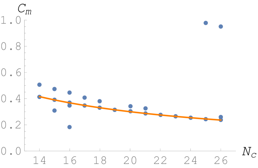
(a) Rewriting values of $C_{\text{m}}$.

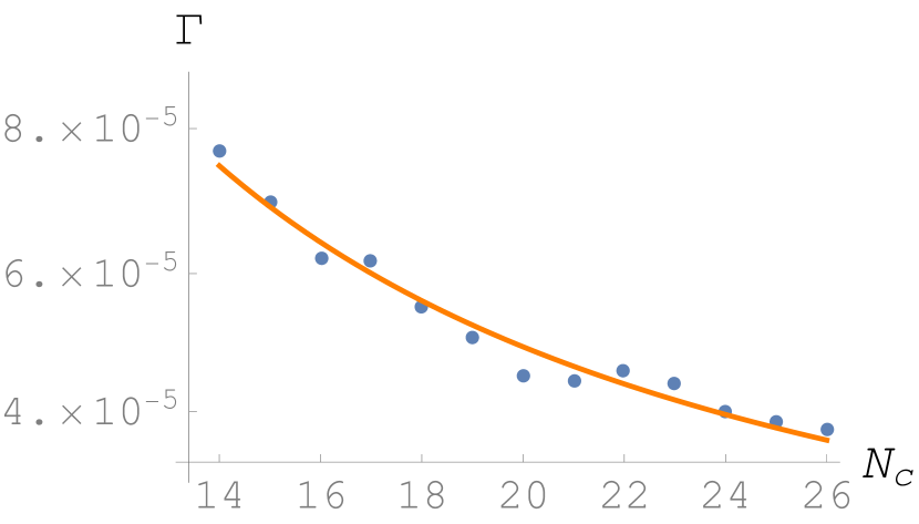
(b) Rates $\Gamma$ at those rewriting values.

Figure 5: Data and fits for the rewriting values of $C_{m}$ and the rates $\Gamma$ as function of $N_{c}$. $\Delta N_{c}$ has been varied to keep $N_{c}/\Delta N_{c}$ fixed.

The data used to determine the scaling of $(C_{m},\Gamma)$ with $N_{c}$ is shown in Fig. 5. The $N_{c}$-variation has been done varying also $\Delta N_{c}$, s.t. $N_{c}/\Delta N_{c}$ stays fixed. The function fitted to the rewriting values is $f_{C}(N_{c})=a\left(\frac{N_{c}}{22}\right)^{-b}$, with the fit result $a\approx 0.275$ and $b\approx 0.911$. The function fitted to the rates is $f_{\Gamma}(N_{c})=A\left(\frac{N_{c}}{22}\right)^{-B}$, with the fit result $A\approx 4.46\cdot 10^{-5}$ and $B\approx 1.14$.

$\epsilon_{m}$-Scaling

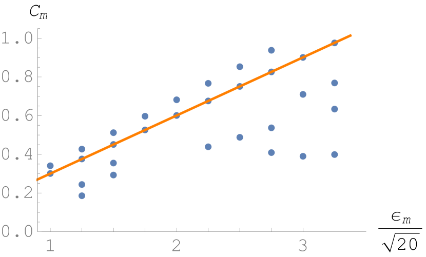
(a) Rewriting values of $C_{\text{m}}$.

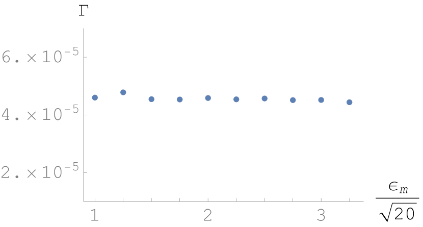
(b) Rates $\Gamma$ at those rewriting values.

Figure 6: Data and fit for the rewriting values of $C_{m}$ and the rates $\Gamma$ as function of $\epsilon_{m}$.

The data used to determine the scaling of $(C_{m},\Gamma)$ with $\epsilon_{m}$ is shown in Fig. 6. The function fitted to the rewriting values is $f_{C}(\epsilon_{m})=a\epsilon_{m}$, with the fit result $a\approx 0.300$. We observe that the scaling of the rate $\Gamma$ with $\epsilon_{m}$ is negligible compared to its scaling with other parameters.

$C_{0}$-Scaling

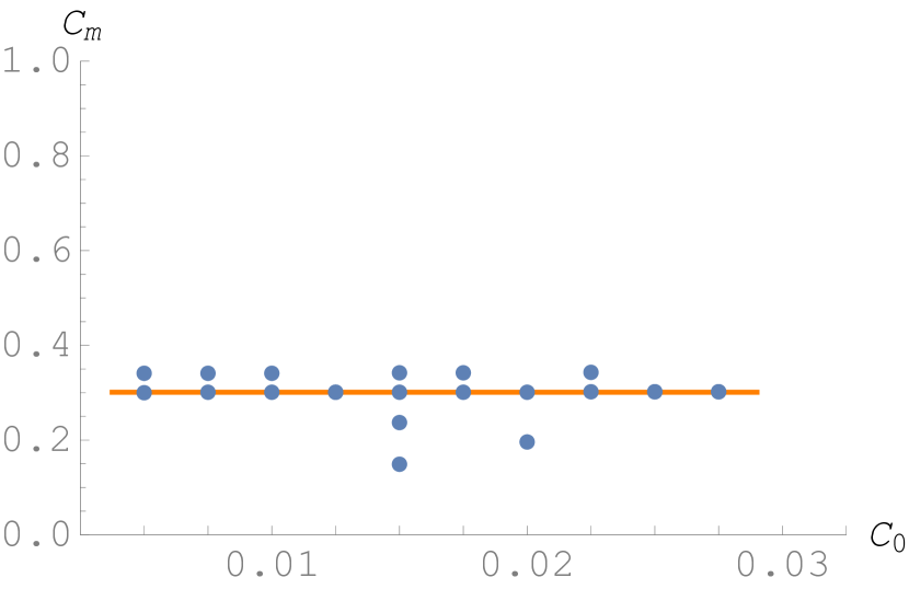
(a) Rewriting values of $C_{\text{m}}$.

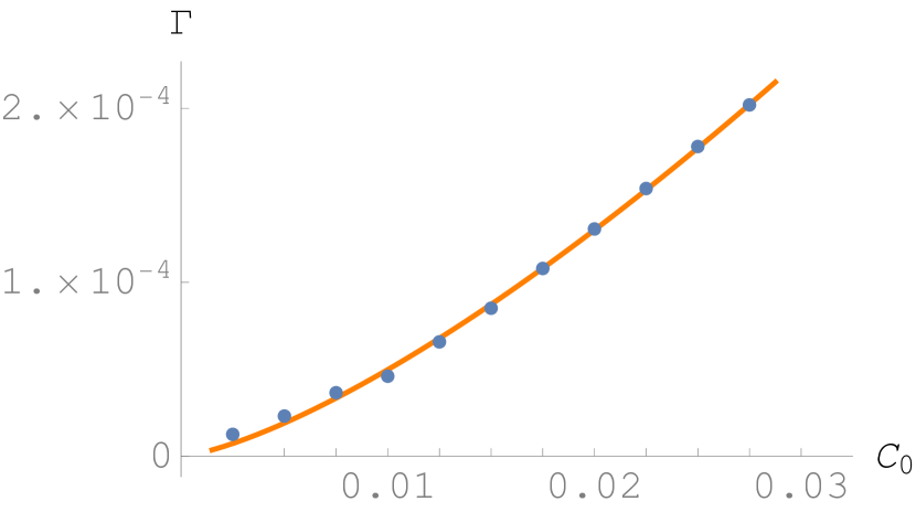
(b) Rates $\Gamma$ at those rewriting values.

Figure 7: Data and fits for the rewriting values of $C_{m}$ and the rates $\Gamma$ as function of $C_{0}$.

The data used to determine the scaling of $(C_{m},\Gamma)$ with $C_{0}$ is shown in Fig. 7. For the scaling of the rewriting values with $C_{0}$, we observe that it is negligible compared to the scaling with other parameters. The function fitted to the rates is $f_{\Gamma}(C_{0})=AC_{0}^{B}$, with the fit result $A\approx 2.85\cdot 10^{-2}$ and $B\approx 1.38$.

$\Delta N_{c}$-Scaling

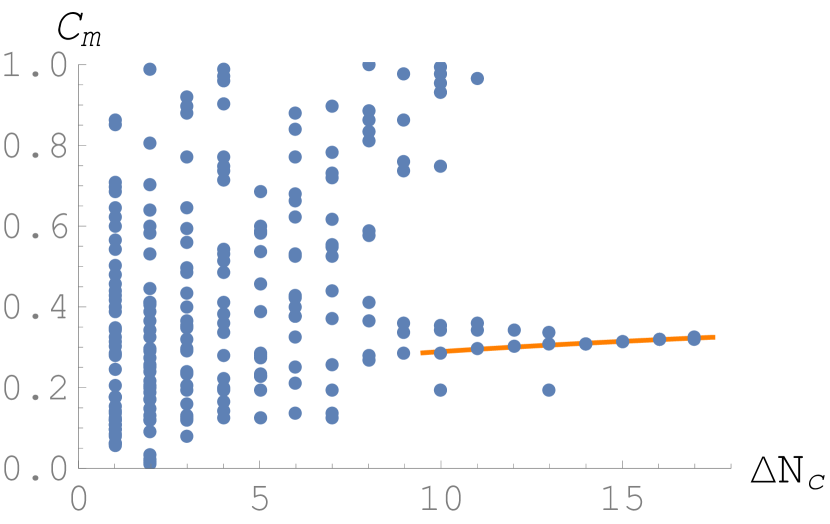
(a) Rewriting values of $C_{\text{m}}$.

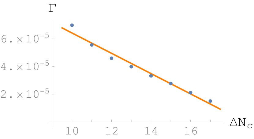
(b) Rates $\Gamma$ at those rewriting values.

Figure 8: Data and fits for the rewriting values of $C_{m}$ and the rates $\Gamma$ as function of $\Delta N_{c}$.

The data used to determine the scaling of $(C_{m},\Gamma)$ with $\Delta N_{c}$ is shown in Fig. 8. The function fitted to the rewriting values is $f_{C}(\Delta N_{c})=a\left(\frac{\Delta N_{c}}{12}\right)^{b}$, with the fit result $a\approx 0.300$ and $b\approx 0.207$. The function fitted to the rates is $f_{\Gamma}(\Delta N_{c})=A\left(1-B\frac{\Delta N_{c}}{20}\right)$, with the fit result $A\approx 1.38\cdot 10^{-4}$ and $B\approx 1.07$.

$K$-Scaling

When investigating how the system depends on $K$, the problem is that the size of the Hilbert space grows exponentially with the number of modes. Therefore, only values up to $K=8$ are numerically accessible. In order to be insensitive to effects of changing the relative occupation of the memory modes, we moreover restrict ourselves to $N_{m}=K/2$. Since the system appears to behave in a non-generic way for $K=2$, we are only left with three datasets corresponding to $K=4,6,8$.

An additional difficulty arises from the fact that time evolutions for $K=8$ are already very time-consuming. Since many rewriting values exist at $K=8$, it is not feasible to perform fine scans, which are required for a precise determination of the rate, around each of them. To overcome this problem, we have selected a particular subset of rewriting values and only used them for the subsequent analysis. Namely, only those rewriting values of $C_{m}$ have been taken into account which have at least one neighboring rewriting value, i.e., a rewriting value separated solely by the increment $\delta C_{m}=10^{-3}$. Of course, we have applied the same selection procedure for $K=4$ and $K=6$. Only the selected rewriting values are displayed in Fig. 4, and only for those the rate has been determined by means of a finer scan.

References

- [1] G. Dvali, A Microscopic Model of Holography: Survival by the Burden of Memory, arXiv:1810.02336 [hep-th] .
- Dvali et al. [2019a] G. Dvali, L. Eisemann, M. Michel, and S. Zell, Universe’s Primordial Quantum Memories, JCAP 1903, 010, arXiv:1812.08749 [hep-th] .
- Dvali and Gomez [2013a] G. Dvali and C. Gomez, Black Hole’s Quantum N-Portrait, Fortsch. Phys. 61, 742 (2013a), arXiv:1112.3359 [hep-th] .
- Dvali and Gomez [2014a] G. Dvali and C. Gomez, Black Holes as Critical Point of Quantum Phase Transition, Eur. Phys. J. C74, 2752 (2014a), arXiv:1207.4059 [hep-th] .
- Dvali et al. [2015] G. Dvali, A. Franca, C. Gomez, and N. Wintergerst, Nambu-Goldstone Effective Theory of Information at Quantum Criticality, Phys. Rev. D92, 125002 (2015), arXiv:1507.02948 [hep-th] .
- Dvali and Panchenko [2015] G. Dvali and M. Panchenko, Black Hole Type Quantum Computing in Critical Bose-Einstein Systems (2015), arXiv:1507.08952 [hep-th] .
- Dvali and Panchenko [2016] G. Dvali and M. Panchenko, Black Hole Based Quantum Computing in Labs and in the Sky, Fortsch. Phys. 64, 569 (2016), arXiv:1601.01329 [hep-th] .
- Dvali [2017] G. Dvali, Critically excited states with enhanced memory and pattern recognition capacities in quantum brain networks: Lesson from black holes (2017), arXiv:1711.09079 [quant-ph] .
- Dvali [2018a] G. Dvali, Black Holes as Brains: Neural Networks with Area Law Entropy, Fortsch. Phys. 66, 1800007 (2018a), arXiv:1801.03918 [hep-th] .
- Dvali [2018b] G. Dvali, Area law microstate entropy from criticality and spherical symmetry, Phys. Rev. D97, 105005 (2018b), arXiv:1712.02233 [hep-th] .
- Dvali et al. [2019b] G. Dvali, M. Michel, and S. Zell, Finding Critical States of Enhanced Memory Capacity in Attractive Cold Bosons, EPJ Quant. Technol. 6, 1 (2019b), arXiv:1805.10292 [quant-ph] .
- Dvali [2019a] G. Dvali, Area Law Saturation of Entropy Bound from Perturbative Unitarity in Renormalizable Theories (2019a), arXiv:1906.03530 [hep-th] .
- Dvali [2019b] G. Dvali, Unitarity Entropy Bound: Solitons and Instantons (2019b), arXiv:1907.07332 [hep-th] .
- Dvali [2020] G. Dvali, Entropy Bound and Unitarity of Scattering Amplitudes (2020), arXiv:2003.05546 [hep-th] .
- Dvali and Gomez [2014b] G. Dvali and C. Gomez, Quantum Compositeness of Gravity: Black Holes, AdS and Inflation, JCAP 1401, 023, arXiv:1312.4795 [hep-th] .
- Dvali and Gomez [2013b] G. Dvali and C. Gomez, Black Hole’s 1/N Hair, Phys. Lett. B719, 419 (2013b), arXiv:1203.6575 [hep-th] .
- Dvali and Gomez [2012a] G. Dvali and C. Gomez, Black Hole Macro-Quantumness (2012a), arXiv:1212.0765 [hep-th] .
- Dvali et al. [2013] G. Dvali, D. Flassig, C. Gomez, A. Pritzel, and N. Wintergerst, Scrambling in the Black Hole Portrait, Phys. Rev. D88, 124041 (2013), arXiv:1307.3458 [hep-th] .
- Dvali et al. [2017] G. Dvali, C. Gomez, and S. Zell, Quantum Break-Time of de Sitter, JCAP 1706, 028, arXiv:1701.08776 [hep-th] .
- Gibbons and Hawking [1977] G. W. Gibbons and S. W. Hawking, Cosmological Event Horizons, Thermodynamics, and Particle Creation, Phys. Rev. D15, 2738 (1977).
- Tao [2012] T. Tao, Topics in Random Matrix Theory, Graduate studies in mathematics, Vol. 132 (AMS, 2012).
- Dvali [2018c] G. Dvali, Classicalization Clearly: Quantum Transition into States of Maximal Memory Storage Capacity (2018c), arXiv:1804.06154 [hep-th] .
- Bekenstein [1973] J. D. Bekenstein, Black holes and entropy, Phys. Rev. D7, 2333 (1973).
- Hawking [1975] S. Hawking, Particle Creation by Black Holes, Commun. Math. Phys. 43, 199 (1975).
- Michel and Zell [2022] M. Michel and S. Zell, : A Program for Time Evolution With Improved Error Bound, Comput. Phys. Commun. 277, 108374 (2022), arXiv:2205.15346 [quant-ph] .
- [26] G. Dvali, L. Eisemann, M. Michel, and S. Zell, Numerical data for ”Black Hole Metamorphosis and Stabilization by Memory Burden [arXiv:2006.00011]”, Zenodo dataset: 10.5281/zenodo.6810715.
- Dvali [2016] G. Dvali, Non-Thermal Corrections to Hawking Radiation Versus the Information Paradox, Fortsch. Phys. 64, 106 (2016), arXiv:1509.04645 [hep-th] .
- Dvali and Gomez [2012b] G. Dvali and C. Gomez, Landau–Ginzburg limit of black hole’s quantum portrait: Self-similarity and critical exponent, Phys. Lett. B716, 240 (2012b), arXiv:1203.3372 [hep-th] .
- Foit and Wintergerst [2015] V. F. Foit and N. Wintergerst, Self-similar Evaporation and Collapse in the Quantum Portrait of Black Holes, Phys. Rev. D92, 064043 (2015), arXiv:1504.04384 [hep-th] .
- Zel’dovich and Novikov [1967] Y. B. Zel’dovich and I. D. Novikov, The Hypothesis of Cores Retarded during Expansion and the Hot Cosmological Model, Sov. Astron. 10, 602 (1967).
- Hawking [1971] S. Hawking, Gravitationally collapsed objects of very low mass, Mon. Not. Roy. Astron. Soc. 152, 75 (1971).
- Carr and Hawking [1974] B. J. Carr and S. Hawking, Black holes in the early Universe, Mon. Not. Roy. Astron. Soc. 168, 399 (1974).
- Chapline [1975] G. F. Chapline, Cosmological effects of primordial black holes, Nature 253, 251 (1975).
- Carr et al. [2016a] B. Carr, F. Kuhnel, and M. Sandstad, Primordial Black Holes as Dark Matter, Phys. Rev. D94, 083504 (2016a), arXiv:1607.06077 [astro-ph.CO] .
- Carr et al. [2020] B. Carr, K. Kohri, Y. Sendouda, and J. Yokoyama, Constraints on Primordial Black Holes (2020), arXiv:2002.12778 [astro-ph.CO] .
- Carr et al. [2016b] B. J. Carr, K. Kohri, Y. Sendouda, and J. Yokoyama, Constraints on primordial black holes from the Galactic gamma-ray background, Phys. Rev. D94, 044029 (2016b), arXiv:1604.05349 [astro-ph.CO] .
- Carr et al. [2010] B. J. Carr, K. Kohri, Y. Sendouda, and J. Yokoyama, New cosmological constraints on primordial black holes, Phys. Rev. D81, 104019 (2010), arXiv:0912.5297 [astro-ph.CO] .
- Alcock et al. [1998] C. Alcock et al. (MACHO, EROS), EROS and MACHO combined limits on planetary mass dark matter in the galactic halo, Astrophys. J. Lett. 499, L9 (1998), arXiv:astro-ph/9803082 [astro-ph] .
- Dvali et al. [2020] G. Dvali, E. Koutsangelas, and F. Kuhnel, Compact Dark Matter Objects via Dark Sectors, Phys. Rev. D101, 083533 (2020), arXiv:1911.13281 [astro-ph.CO] .
- Ackermann et al. [2015] M. Ackermann et al. (Fermi-LAT), The spectrum of isotropic diffuse gamma-ray emission between 100 MeV and 820 GeV, Astrophys. J. 799, 86 (2015), arXiv:1410.3696 [astro-ph.HE] .
- Kneiske et al. [2001] T. Kneiske, K. Mannheim, and D. Hartmann, The Gamma-ray horizon, AIP Conf. Proc. 587, 358 (2001).
- Luo et al. [2012] Y. Luo, S. Hanasoge, J. Tromp, and F. Pretorius, Detectable seismic consequences of the interaction of a primordial black hole with Earth, Astrophys. J. 751, 16 (2012), arXiv:1203.3806 [astro-ph.CO] .
- Page [1993] D. N. Page, Information in black hole radiation, Phys. Rev. Lett. 71, 3743 (1993), arXiv:hep-th/9306083 [hep-th] .
- Ruffini and Wheeler [1971] R. Ruffini and J. A. Wheeler, Introducing the black hole, Phys. Today 24, 30 (1971).
- Hartle [1971] J. B. Hartle, Long-range neutrino forces exerted by kerr black holes, Phys. Rev. D3, 2938 (1971).
- Bekenstein [1972a] J. D. Bekenstein, Transcendence of the law of baryon-number conservation in black hole physics, Phys. Rev. Lett. 28, 452 (1972a).
- Bekenstein [1972b] J. D. Bekenstein, Nonexistence of baryon number for static black holes, Phys. Rev. D5, 1239 (1972b).
- Bekenstein [1972c] J. D. Bekenstein, Nonexistence of baryon number for black holes. ii, Phys. Rev. D5, 2403 (1972c).
- Teitelboim [1972a] C. Teitelboim, Nonmeasurability of the baryon number of a black-hole, Lett. Nuovo Cim. 3, 326 (1972a).
- Teitelboim [1972b] C. Teitelboim, Nonmeasurability of the lepton number of a black hole, Lett. Nuovo Cim. 3, 397 (1972b).