Supplementary Materials

Section S1. Description of the sensor-target system

The target spin consists of a spin-1/2 electron spin and a spin-1/2 nuclear spin. At zero magnetic field, only the hyperfine interaction is included, and thus the Hamiltonian can be written as

$$H_{\text{t}}=\mathbf{S}\cdot\mathbf{A}\cdot\mathbf{I},$$ (S1)

where $\mathbf{A}$ is the hyperfine tensor, and is diagonal

$$\mathbf{A}=\left(\begin{array}[]{ccc}A_{\perp}&&\\ &A_{\perp}&\\ &&A_{\parallel}\end{array}\right)$$ (S2)

in the principal axis frame. $\mathbf{S}$ and $\mathbf{I}$ are the electron and nuclear spin operators, respectively. To conveniently describe this system, we transform the bare spin-up and spin-down basis to the spin singlet and triplet basis $\{|T_{+1}\rangle,|S_{0}\rangle,|T_{0}\rangle,|T_{-1}\rangle\}$:

$$\begin{split}&|T_{+1}\rangle=|\uparrow\uparrow\rangle,\\ &|S_{0}\rangle=\frac{1}{\sqrt{2}}(|\uparrow\downarrow\rangle-|\downarrow\uparrow\rangle),\\ &|T_{0}\rangle=\frac{1}{\sqrt{2}}(|\uparrow\downarrow\rangle+|\downarrow\uparrow\rangle),\\ &|T_{-1}\rangle=|\downarrow\downarrow\rangle,\\ \end{split}$$ (S3)

and then Eq. S1 can be diagonalized as

$$H_{\text{t}}^{\mathcal{T}}=\mathcal{T}\cdot H_{\text{t}}\cdot\mathcal{T}^{-1}=\frac{1}{4}\left(\begin{array}[]{cccc}A_{\parallel}&&&\\ &-A_{\parallel}-2A_{\perp}&&\\ &&-A_{\parallel}+2A_{\perp}&\\ &&&A_{\parallel}\end{array}\right),$$ (S4)

where

$$\mathcal{T}=\begin{pmatrix}1&0&0&0\\ 0&\frac{1}{\sqrt{2}}&-\frac{1}{\sqrt{2}}&0\\ 0&\frac{1}{\sqrt{2}}&\frac{1}{\sqrt{2}}&0\\ 0&0&0&1\end{pmatrix}$$ (S5)

is the transformation matrix. The eigenenergies of the target spin, $\omega_{T_{+1}}$, $\omega_{S_{0}}$, $\omega_{T_{0}}$, and $\omega_{T_{-1}}$, are just the diagonal elements in Eq. S4. In this new basis, the electron spin operators can be written as

$$\begin{split}&S_{x}^{\mathcal{T}}=\mathcal{T}\cdot(S_{x}\otimes I_{2})\cdot\mathcal{T}^{-1}=\frac{1}{2\sqrt{2}}\begin{pmatrix}0&-1&1&0\\ -1&0&0&1\\ 1&0&0&1\\ 0&1&1&0\end{pmatrix},\\ &S_{y}^{\mathcal{T}}=\mathcal{T}\cdot(S_{y}\otimes I_{2})\cdot\mathcal{T}^{-1}=\frac{1}{2\sqrt{2}}\begin{pmatrix}0&\text{i}&-\text{i}&0\\ -\text{i}&0&0&-\text{i}\\ \text{i}&0&0&-\text{i}\\ 0&\text{i}&\text{i}&0\end{pmatrix},\\ &S_{z}^{\mathcal{T}}=\mathcal{T}\cdot(S_{z}\otimes I_{2})\cdot\mathcal{T}^{-1}=\frac{1}{2}\begin{pmatrix}1&0&0&0\\ 0&0&1&0\\ 0&1&0&0\\ 0&0&0&-1\end{pmatrix},\end{split}$$ (S6)

where $I_{2}$ is the $2\times 2$ identity matrix. The nuclear spin operators can be transformed in a similar way, but are ignored due to the much smaller gyromagnetic ratio.

The Hamiltonian of magnetic noise can also be written in the new basis as

$$\delta H^{\mathcal{T}}=\sum_{j=x,y,z}\delta_{j}S_{j}^{\mathcal{T}}.$$ (S7)

It can be diagonalized according to the perturbation theory:

$$\delta H_{0}^{\mathcal{T}}=\begin{pmatrix}\delta\omega_{T_{+1}}&0&0&0\\ 0&\delta\omega_{S_{0}}&0&0\\ 0&0&\delta\omega_{T_{0}}&0\\ 0&0&0&\delta\omega_{T_{-1}}\end{pmatrix},$$ (S8)

where the energy level shifts are

$$\begin{split}&\delta\omega_{T_{+1}}=\frac{\delta_{z}}{2}+O(\delta^{2}),\\ &\delta\omega_{S_{0}}=-\frac{{\delta_{x}}^{2}+{\delta_{y}}^{2}}{2(A_{\parallel}+A_{\perp})}-\frac{{\delta_{z}}^{2}}{4A_{\perp}}+O(\delta^{4}),\\ &\delta\omega_{T_{0}}=-\frac{{\delta_{x}}^{2}+{\delta_{y}}^{2}}{2(A_{\parallel}-A_{\perp})}+\frac{{\delta_{z}}^{2}}{4A_{\perp}}+O(\delta^{4}),\\ &\delta\omega_{T_{-1}}=-\frac{\delta_{z}}{2}+O(\delta^{2}).\end{split}$$ (S9)

If we apply a radiofrequency (RF) pulse perpendicular to the principle axis with frequency $\omega_{\text{ST}_{\pm 1}}=|\omega_{S_{0}}-\omega_{T_{\pm 1}}|$, for example, of the form $H_{1,\text{t}}=2\Omega_{x}\cos{(\omega_{\text{ST}_{\pm 1}}t)}S_{x}^{\mathcal{T}}$, then a transition between $|S_{0}\rangle\leftrightarrow|T_{\pm 1}\rangle$ will happen. The transition operator can be written as

$$U_{\text{ST}_{\pm 1}}^{\mathcal{T}}(\theta)=\begin{pmatrix}\frac{1+\cos{\frac{\theta}{2}}}{2}&\frac{\text{i}\sin{\frac{\theta}{2}}}{\sqrt{2}}&0&\frac{1-\cos{\frac{\theta}{2}}}{2}\\ \frac{\text{i}\sin{\frac{\theta}{2}}}{\sqrt{2}}&\cos{\frac{\theta}{2}}&0&-\frac{\text{i}\sin{\frac{\theta}{2}}}{\sqrt{2}}\\ 0&0&1&0\\ \frac{1-\cos{\frac{\theta}{2}}}{2}&-\frac{\text{i}\sin{\frac{\theta}{2}}}{\sqrt{2}}&0&\frac{1+\cos{\frac{\theta}{2}}}{2}\end{pmatrix},$$ (S10)

where $\theta=\Omega_{x}t_{\text{RF}}$, $t_{\text{RF}}$ is the pulse length. Specifically, the operators of $\pi$ and $2\pi$ pulses are

$$U_{\text{ST}_{\pm 1}}^{\mathcal{T}}(\pi)=\begin{pmatrix}\frac{1}{2}&\frac{\text{i}}{\sqrt{2}}&0&\frac{1}{2}\\ \frac{\text{i}}{\sqrt{2}}&0&0&-\frac{\text{i}}{\sqrt{2}}\\ 0&0&1&0\\ \frac{1}{2}&-\frac{\text{i}}{\sqrt{2}}&0&\frac{1}{2}\end{pmatrix},U_{\text{ST}_{\pm 1}}^{\mathcal{T}}(2\pi)=\begin{pmatrix}0&0&0&1\\ 0&-1&0&0\\ 0&0&1&0\\ 1&0&0&0\end{pmatrix}.$$ (S11)

Similarly, a RF pulse parallel to the principle axis with frequency $\omega_{\text{ST}_{0}}=|\omega_{S_{0}}-\omega_{T_{0}}|$ will induce transition between $|S_{0}\rangle\leftrightarrow|T_{0}\rangle$, and the corresponding transition operator is

$$U_{\text{ST}_{0}}^{\mathcal{T}}(\theta)=\begin{pmatrix}1&0&0&0\\ 0&\cos{\frac{\theta}{2}}&-\text{i}\sin{\frac{\theta}{2}}&0\\ 0&-\text{i}\sin{\frac{\theta}{2}}&\cos{\frac{\theta}{2}}&0\\ 0&0&0&1\end{pmatrix}.$$ (S12)

The transition between $|T_{0}\rangle\leftrightarrow|T_{\pm 1}\rangle$ can also be driven by perpendicular RF with the corresponding resonant frequency, but has not been involved in our experiments.

At zero magnetic field, the Hamiltonian of NV centers can be written as

$$H_{\text{NV}}=D{S_{z}^{\text{NV}}}^{2},$$ (S13)

where $D=2.87$ GHz is the zero-field splitting of the NV center, $\mathbf{S}^{\text{NV}}$ is the spin-1 operator for the NV electron spin.

The dipole-dipole coupling between the NV center and the target spin can be written as

$$H_{\text{dd}}=\frac{\mu_{0}\gamma_{\text{NV}}\gamma_{\text{tar}}\hbar}{4\pi}[\frac{\mathbf{S}^{\text{NV}}\cdot\mathbf{S}^{\text{tar}}}{r^{3}}-\frac{3(\mathbf{S}^{\text{NV}}\cdot\mathbf{r})(\mathbf{r}\cdot\mathbf{S}^{\text{tar}})}{r^{5}}],$$ (S14)

where $\gamma_{\text{NV}}$ and $\gamma_{\text{tar}}$ are the gyromagnetic ratios of the NV and target electron spin, respectively. $\mathbf{S}^{\text{NV}}$ and $\mathbf{S}^{\text{tar}}$ are the spin operators of the NV and target electron spin, respectively. $\mathbf{r}$ is the separation vector between the sensor and the target. Here all the vectors are defined in the NV frame with the $z$ axis towards the N-V axis, where $\mathbf{r}$ and the principal axis of the target spin are characterized by $\{\theta_{r},\phi_{r}\}$ and $\{\theta_{\text{e}},\phi_{\text{e}}\}$, respectively. The transformation from the principle axis frame to the NV frame can be represented by a rotation matrix:

$$\mathcal{R}=\begin{pmatrix}\cos{\theta_{\text{e}}}\cos{\phi_{\text{e}}}&-\sin{\phi_{\text{e}}}&\sin{\theta_{\text{e}}}\cos{\phi_{\text{e}}}\\ \cos{\theta_{\text{e}}}\sin{\phi_{\text{e}}}&\cos{\phi_{\text{e}}}&\sin{\theta_{\text{e}}}\sin{\phi_{\text{e}}}\\ -\sin{\theta_{\text{e}}}&0&\cos{\theta_{\text{e}}}\end{pmatrix}.$$ (S15)

Then, we have

$$\mathbf{S}^{\text{tar}}=\mathcal{R}\cdot\mathbf{S}^{\mathcal{T}},$$ (S16)

here $\mathbf{S}^{\mathcal{T}}$ is defined in Eq. S6. Such coupling is usually a small perturbation to the Hamiltonian of the NV center (Eq. S13) and the target spin (Eq. S4), so the secular approximation can be performed, and Eq. S14 can be simplified to

$$\begin{split}H_{\text{dd}}&\approx\frac{\mu_{0}\gamma_{\text{NV}}\gamma_{\text{tar}}\hbar}{4\pi r^{3}}(\cos{\theta_{\text{e}}}-3\cos{\theta_{r}}\cos{\theta_{r^{{}^{\prime}}}})S_{z}^{\text{NV}}S_{zz}^{\mathcal{T}}\\ &=C(\theta_{\text{e}},r,\theta_{r},\theta_{r^{{}^{\prime}}})S_{z}^{\text{NV}}S_{zz}^{\mathcal{T}},\end{split}$$ (S17)

where $\theta_{r^{{}^{\prime}}}$ is the angle between $\mathbf{r}$ and the principal axis, and $S_{zz}^{\mathcal{T}}$ is a simplified form of $S_{z}^{\mathcal{T}}$:

$$S_{zz}^{\mathcal{T}}=\frac{1}{2}\begin{pmatrix}1&&&\\ &0&&\\ &&0&\\ &&&-1\end{pmatrix}$$ (S18)

Section S2. Calculations of DEER signal

The DEER signal is determined by the accumulated phase $\phi=a\cdot\tau$, where $a$ is the dipolar coupling strength, depending on the state of the target spin according to Eq. S17. The target spin is in thermal equilibrium, which means it has nearly equal probability in $|T_{+1}\rangle$, $|S_{0}\rangle$, $|T_{0}\rangle$, and $|T_{-1}\rangle$ states. To quantitatively describe the zero-field DEER signal, we disassemble the evolution as following:

Transition		Accumulated phase $\phi$
$|T_{+1}\rangle\xrightarrow{U_{\text{ST}_{\pm 1}}^{\mathcal{T}}(\theta)}$	$(\frac{1}{2}+\frac{1}{2}\cos{\frac{\theta}{2}})|T_{+1}\rangle$	0
	$+\frac{\text{i}}{\sqrt{2}}\sin{\frac{\theta}{2}}|S_{0}\rangle$	$\frac{1}{4}C\tau$
	$+(\frac{1}{2}-\frac{1}{2}\cos{\frac{\theta}{2}})|T_{-1}\rangle$	$\frac{1}{2}C\tau$
$|S_{0}\rangle\xrightarrow{U_{\text{ST}_{\pm 1}}^{\mathcal{T}}(\theta)}$	$\frac{\text{i}}{\sqrt{2}}\sin{\frac{\theta}{2}}|T_{+1}\rangle$	$-\frac{1}{4}C\tau$
	$+\cos{\frac{\theta}{2}}|S_{0}\rangle$	0
	$-\frac{\text{i}}{\sqrt{2}}\sin{\frac{\theta}{2}}|T_{-1}\rangle$	$\frac{1}{4}C\tau$
$|T_{0}\rangle\xrightarrow{U_{\text{ST}_{\pm 1}}^{\mathcal{T}}(\theta)}$	$|T_{0}\rangle$	0
$|T_{-1}\rangle\xrightarrow{U_{\text{ST}_{\pm 1}}^{\mathcal{T}}(\theta)}$	$(\frac{1}{2}-\frac{1}{2}\cos{\frac{\theta}{2}})|T_{+1}\rangle$	$-\frac{1}{2}C\tau$
	$+\frac{\text{i}}{\sqrt{2}}\sin{\frac{\theta}{2}}|S_{0}\rangle$	$-\frac{1}{4}C\tau$
	$+(\frac{1}{2}+\frac{1}{2}\cos{\frac{\theta}{2}})|T_{-1}\rangle$	0

The signal can be calculated as the weighted average of each rows, which is

$$\begin{split}S(\theta,\tau)&=\langle\cos^{2}{\phi}\rangle\\ &=\frac{1}{32}[25+3\cos{\theta}+4\cos{\frac{\theta}{2}}+4(1-\cos{\theta})\cos{\frac{C\tau}{2}}+2(1-\cos{\frac{\theta}{2}})^{2}\cos{C\tau}]\\ &=\frac{1}{32}[25+3\cos{C\tau}+4\cos{\frac{C\tau}{2}}+4(1-\cos{C\tau})\cos{\frac{\theta}{2}}+2(1-\cos{\frac{C\tau}{2}})^{2}\cos{\theta}].\end{split}$$ (S19)

In general, one can see an dual-frequency oscillation by varying the RF pulse length, i.e., $\theta$, with fixed evolution time $\tau$, and vice versa. However, a better strategy is utilizing the faster term in $\tau$ domain because of the decoherence process during the evolution. So we choose $2\pi$ RF pulse rather than $\pi$ RF pulse, and then the zero-field DEER signal can be simplified as $(3+\cos{C\tau})/4$. Due to the decoherence, there will be an extra random phase $\delta\phi(\tau)$ accumulated during the evolution. The average effect of this random phase is a stretched exponential decay, and thus the signal can be written as

$$S(\tau)=\frac{3}{4}+\frac{1}{4}e^{-(\tau/T_{2,\text{NV}})^{p}}\cos{C\tau},$$ (S20)

where $p$ is in the range of $1-3$ determined by the dynamic of bath.

Section S3. Correlation Rabi measurement

To see how the manipulation of the target spin during spin-locking period (the black dash box in Fig. 2a in the main text) affects the correlation signal, we use a similar strategy described above to disassemble the evolution. First, we write the operator of the manipulation. For example, the operator corresponding to $\text{ST}_{\pm 1}$ Rabi oscillation (Fig. 2b in the main text) is $U_{\text{Rabi},\text{ST}_{\pm 1}}=U_{\text{ST}_{\pm 1}}^{\mathcal{T}}(\theta)$ given by Eq. S10. Then, the evolution is disassembled:

Evolution of the target spin			$\phi_{1}$	$\phi_{2}$
$|T_{+1}\rangle\xrightarrow{2\pi}|T_{-1}\rangle\xrightarrow{U}$	$(\frac{1}{2}-\frac{1}{2}\cos{\frac{\theta}{2}})|T_{+1}\rangle$	$\xrightarrow{2\pi}|T_{-1}\rangle$	$\frac{1}{2}C\tau$	$\frac{1}{2}C\tau$
	$+\frac{\text{i}}{\sqrt{2}}\sin{\frac{\theta}{2}}|S_{0}\rangle$	$\xrightarrow{2\pi}|S_{0}\rangle$	$\frac{1}{2}C\tau$	0
	$+(\frac{1}{2}+\frac{1}{2}\cos{\frac{\theta}{2}})|T_{-1}\rangle$	$\xrightarrow{2\pi}|T_{+1}\rangle$	$\frac{1}{2}C\tau$	$-\frac{1}{2}C\tau$
$|S_{0}\rangle\xrightarrow{2\pi}|S_{0}\rangle\xrightarrow{U}$	$+\frac{\text{i}}{\sqrt{2}}\sin{\frac{\theta}{2}}|T_{+1}\rangle$	$\xrightarrow{2\pi}|T_{-1}\rangle$	0	$\frac{1}{2}C\tau$
	$+\cos{\frac{\theta}{2}}|S_{0}\rangle$	$\xrightarrow{2\pi}|S_{0}\rangle$	0	0
	$-\frac{\text{i}}{\sqrt{2}}\sin{\frac{\theta}{2}}|T_{-1}\rangle$	$\xrightarrow{2\pi}|T_{+1}\rangle$	0	$-\frac{1}{2}C\tau$
$|T_{0}\rangle\xrightarrow{2\pi}|T_{0}\rangle\xrightarrow{U}$	$|T_{0}\rangle$	$\xrightarrow{2\pi}|T_{0}\rangle$	0	0
$|T_{-1}\rangle\xrightarrow{2\pi}|T_{+1}\rangle\xrightarrow{U}$	$(\frac{1}{2}+\frac{1}{2}\cos{\frac{\theta}{2}})|T_{+1}\rangle$	$\xrightarrow{2\pi}|T_{-1}\rangle$	$-\frac{1}{2}C\tau$	$\frac{1}{2}C\tau$
	$+\frac{\text{i}}{\sqrt{2}}\sin{\frac{\theta}{2}}|S_{0}\rangle$	$\xrightarrow{2\pi}|S_{0}\rangle$	$-\frac{1}{2}C\tau$	0
	$+(\frac{1}{2}-\frac{1}{2}\cos{\frac{\theta}{2}})|T_{-1}\rangle$	$\xrightarrow{2\pi}|T_{+1}\rangle$	$-\frac{1}{2}C\tau$	$-\frac{1}{2}C\tau$

The corresponding correlation signal is

$$\boxed{S_{\text{Rabi},\text{ST}_{\pm 1}}\sim\langle\cos{2\phi_{1}}\cos{2\phi_{2}}\rangle=\frac{1}{8}(1-\cos{C\tau})^{2}\cos{\theta}+\frac{3}{8}+\frac{1}{4}\cos{C\tau}+\frac{3}{8}\cos^{2}{C\tau},}$$ (S21)

which is a single-frequency oscillation. The operator corresponding to $\text{ST}_{0}$ Rabi oscillation (Fig. 2c in the main text) is

$$U_{\text{Rabi},\text{ST}_{0}}=U_{\text{ST}_{\pm 1}}^{\mathcal{T}}(\pi)\cdot U_{\text{ST}_{0}}^{\mathcal{T}}(\theta)\cdot U_{\text{ST}_{\pm 1}}^{\mathcal{T}}(\pi)=\begin{pmatrix}\frac{1-\cos{\frac{\theta}{2}}}{2}&0&\frac{\sin{\frac{\theta}{2}}}{\sqrt{2}}&\frac{1+\cos{\frac{\theta}{2}}}{2}\\ 0&-1&0&0\\ \frac{\sin{\frac{\theta}{2}}}{\sqrt{2}}&0&\cos{\frac{\theta}{2}}&-\frac{\sin{\frac{\theta}{2}}}{\sqrt{2}}\\ \frac{1+\cos{\frac{\theta}{2}}}{2}&0&-\frac{\sin{\frac{\theta}{2}}}{\sqrt{2}}&\frac{1-\cos{\frac{\theta}{2}}}{2}\end{pmatrix},$$ (S22)

and the correlation signal can be calculated in a similar way, which is

$$\boxed{S_{\text{Rabi},\text{ST}_{0}}\sim\langle\cos{2\phi_{1}}\cos{2\phi_{2}}\rangle=\frac{1}{8}(1-\cos{C\tau})^{2}\cos{\theta}+\frac{3}{8}+\frac{1}{4}\cos{C\tau}+\frac{3}{8}\cos^{2}{C\tau}.}$$ (S23)

Section S4. Correlation Ramsey measurement

The operators corresponding to $\text{ST}_{\pm 1}$ Ramsey measurement (Fig. 3a in the main text) are

$$\begin{split}U_{\text{Ramsey},\text{ST}_{\pm 1}}^{\text{sig}}&=U_{\text{ST}_{\pm 1}}^{\mathcal{T}}(-\frac{\pi}{2})\cdot\exp[-\text{i}(H_{\text{t}}^{\mathcal{T}}+\delta H_{0}^{\mathcal{T}})t]\cdot U_{\text{ST}_{\pm 1}}^{\mathcal{T}}(\frac{\pi}{2})\\ &=U_{\text{phase}}\cdot\begin{pmatrix}\frac{1}{4}(1+\alpha e^{-\text{i}\varphi})&\frac{\text{i}\sqrt{2}}{4}(-1+\beta e^{-\text{i}\varphi})&0&\frac{1}{4}(-1+\gamma e^{-\text{i}\varphi})\\ \frac{\text{i}\sqrt{2}}{4}(-1+\beta e^{-\text{i}\varphi})&\frac{1}{2}(1+\gamma e^{-\text{i}\varphi})&0&\frac{\text{i}\sqrt{2}}{4}(-1+\beta^{*}e^{-\text{i}\varphi})\\ 0&0&1&0\\ \frac{1}{4}(-1+\gamma e^{-\text{i}\varphi})&\frac{\text{i}\sqrt{2}}{4}(-1+\beta^{*}e^{-\text{i}\varphi})&0&\frac{1}{4}(1+\alpha^{*}e^{-\text{i}\varphi})\end{pmatrix},\end{split}$$ (S24)

and

$$\begin{split}U_{\text{Ramsey},\text{ST}_{\pm 1}}^{\text{ref}}&=U_{\text{ST}_{\pm 1}}^{\mathcal{T}}(\frac{\pi}{2})\cdot\exp[-\text{i}(H_{\text{t}}^{\mathcal{T}}+\delta H_{0}^{\mathcal{T}})t]\cdot U_{\text{ST}_{\pm 1}}^{\mathcal{T}}(\frac{\pi}{2})\\ &=U_{\text{phase}}\cdot\begin{pmatrix}\frac{1}{4}(-1+\alpha e^{-\text{i}\varphi})&\frac{\text{i}\sqrt{2}}{4}(1+\beta e^{-\text{i}\varphi})&0&\frac{1}{4}(1+\gamma e^{-\text{i}\varphi})\\ \frac{\text{i}\sqrt{2}}{4}(1+\beta e^{-\text{i}\varphi})&\frac{1}{2}(1-\gamma e^{-\text{i}\varphi})&0&\frac{\text{i}\sqrt{2}}{4}(-1-\beta^{*}e^{-\text{i}\varphi})\\ 0&0&1&0\\ \frac{1}{4}(1+\gamma e^{-\text{i}\varphi})&\frac{\text{i}\sqrt{2}}{4}(-1-\beta^{*}e^{-\text{i}\varphi})&0&\frac{1}{4}(-1+\alpha^{*}e^{-\text{i}\varphi})\end{pmatrix},\end{split}$$ (S25)

where $H_{\text{t}}^{\mathcal{T}}$ and $\delta H_{0}^{\mathcal{T}}$ are given by Eq. S4 and Eq. S8, respectively, the phase operator $U_{\text{phase}}$ can be ignored, $\varphi=\omega_{\text{ST}_{\pm 1}}t$, and the three coefficients are

$$\begin{split}\alpha&=3\cos(\delta\omega_{\text{ST}_{\pm 1}}t)-\text{i}2\sqrt{2}\sin(\delta\omega_{\text{ST}_{\pm 1}}t),\\ \beta&=\cos(\delta\omega_{\text{ST}_{\pm 1}}t)-\text{i}\sqrt{2}\sin(\delta\omega_{\text{ST}_{\pm 1}}t),\\ \gamma&=\cos(\delta\omega_{\text{ST}_{\pm 1}}t).\end{split}$$ (S26)

Then, the signal and reference are

$$\begin{split}S_{\text{Ramsey},\text{ST}_{\pm 1}}^{\text{sig}}&\sim\langle\cos{2\phi_{1}}\cos{2\phi_{2}}\rangle\\ &=\frac{1}{8}(1-\cos{C\tau})^{2}\langle\cos(\delta\omega_{\text{ST}_{\pm 1}}t)\rangle\cos(\omega_{\text{ST}_{\pm 1}}t)\\ &+\frac{1}{32}(1-\cos{C\tau})^{2}\langle\cos(2\delta\omega_{\text{ST}_{\pm 1}}t)\rangle+\frac{11}{32}+\frac{5}{16}\cos{C\tau}+\frac{11}{32}\cos^{2}{C\tau},\end{split}$$ (S27)

and

$$\begin{split}S_{\text{Ramsey},\text{ST}_{\pm 1}}^{\text{ref}}&\sim\langle\cos{2\phi_{1}}\cos{2\phi_{2}}\rangle\\ &=-\frac{1}{8}(1-\cos{C\tau})^{2}\langle\cos(\delta\omega_{\text{ST}_{\pm 1}}t)\rangle\cos(\omega_{\text{ST}_{\pm 1}}t)\\ &+\frac{1}{32}(1-\cos{C\tau})^{2}\langle\cos(2\delta\omega_{\text{ST}_{\pm 1}}t)\rangle+\frac{11}{32}+\frac{5}{16}\cos{C\tau}+\frac{11}{32}\cos^{2}{C\tau},\end{split}$$ (S28)

respectively. The measured differential signal is

$$\boxed{S_{\text{Ramsey},\text{ST}_{\pm 1}}=S_{\text{Ramsey},\text{ST}_{\pm 1}}^{\text{sig}}-S_{\text{Ramsey},\text{ST}_{\pm 1}}^{\text{ref}}\sim\frac{1}{4}(1-\cos{C\tau})^{2}\langle\cos(\delta\omega_{\text{ST}_{\pm 1}}t)\rangle\cos(\omega_{\text{ST}_{\pm 1}}t).}$$ (S29)

Similarly, the operators corresponding to $\text{ST}_{0}$ Ramsey measurement (Fig. 3b in the main text) is

$$\begin{split}U_{\text{Ramsey},\text{ST}_{0}}^{\text{sig}}&=U_{\text{ST}_{\pm 1}}^{\mathcal{T}}(\pi)\cdot U_{\text{ST}_{0}}^{\mathcal{T}}(-\frac{\pi}{2})\cdot\exp[-\text{i}(H_{\text{t}}^{\mathcal{T}}+\delta H_{0}^{\mathcal{T}})t]\cdot U_{\text{ST}_{0}}^{\mathcal{T}}(\frac{\pi}{2})\cdot U_{\text{ST}_{\pm 1}}^{\mathcal{T}}(\pi)\\ &=U_{\text{phase}}\cdot\begin{pmatrix}\frac{1}{2}(\xi\cos{\delta\varphi}-\cos{\frac{\varphi{{}^{\prime}}}{2}})&\frac{1}{\sqrt{2}}\xi\sin{\delta\varphi}&\frac{\text{i}}{\sqrt{2}}\sin{\frac{\varphi{{}^{\prime}}}{2}}&\frac{1}{2}(\xi\cos{\delta\varphi}+\cos{\frac{\varphi{{}^{\prime}}}{2}})\\ \frac{1}{\sqrt{2}}\xi\sin{\delta\varphi}&-\xi\cos{\delta\varphi}&0&\frac{1}{\sqrt{2}}\xi\sin{\delta\varphi}\\ -\frac{\text{i}}{\sqrt{2}}\sin{\frac{\varphi{{}^{\prime}}}{2}}&0&\cos{\frac{\varphi{{}^{\prime}}}{2}}&\frac{\text{i}}{\sqrt{2}}\sin{\frac{\varphi{{}^{\prime}}}{2}}\\ \frac{1}{2}(\xi\cos{\delta\varphi}+\cos{\frac{\varphi{{}^{\prime}}}{2}})&\frac{1}{\sqrt{2}}\xi\sin{\delta\varphi}&-\frac{\text{i}}{\sqrt{2}}\sin{\frac{\varphi{{}^{\prime}}}{2}}&\frac{1}{2}(\xi\cos{\delta\varphi}-\cos{\frac{\varphi{{}^{\prime}}}{2}})\end{pmatrix},\end{split}$$ (S30)

and

$$\begin{split}U_{\text{Ramsey},\text{ST}_{0}}^{\text{ref}}&=U_{\text{ST}_{\pm 1}}^{\mathcal{T}}(\pi)\cdot U_{\text{ST}_{0}}^{\mathcal{T}}(\frac{\pi}{2})\cdot\exp[-\text{i}(H_{\text{t}}^{\mathcal{T}}+\delta H_{0}^{\mathcal{T}})t]\cdot U_{\text{ST}_{0}}^{\mathcal{T}}(\frac{\pi}{2})\cdot U_{\text{ST}_{\pm 1}}^{\mathcal{T}}(\pi)\\ &=U_{\text{phase}}\cdot\begin{pmatrix}\frac{1}{2}(\zeta\cos{\delta\varphi}-\eta\sin{\frac{\varphi{{}^{\prime}}}{2}})&\frac{1}{\sqrt{2}}\xi\sin{\delta\varphi}&\frac{1}{\sqrt{2}}\cos{\frac{\varphi{{}^{\prime}}}{2}}&\frac{1}{2}(\zeta\cos{\delta\varphi}+\eta\sin{\frac{\varphi{{}^{\prime}}}{2}})\\ \frac{1}{\sqrt{2}}\xi\sin{\delta\varphi}&-\xi\cos{\delta\varphi}&0&\frac{1}{\sqrt{2}}\xi\sin{\delta\varphi}\\ \frac{1}{\sqrt{2}}\cos{\frac{\varphi{{}^{\prime}}}{2}}&0&-\text{i}\sin{\frac{\varphi{{}^{\prime}}}{2}}&-\frac{1}{\sqrt{2}}\cos{\frac{\varphi{{}^{\prime}}}{2}}\\ \frac{1}{2}(\zeta\cos{\delta\varphi}+\eta\sin{\frac{\varphi{{}^{\prime}}}{2}})&\frac{1}{\sqrt{2}}\xi\sin{\delta\varphi}&\frac{1}{\sqrt{2}}\cos{\frac{\varphi{{}^{\prime}}}{2}}&\frac{1}{2}(\zeta\cos{\delta\varphi}-\eta\sin{\frac{\varphi{{}^{\prime}}}{2}})\end{pmatrix},\end{split}$$ (S31)

where $\varphi{{}^{\prime}}=(\omega_{\text{ST}_{0}}+\delta\omega_{\text{ST}_{0}})t$, $\delta\varphi=2\delta\omega_{\text{ST}_{\pm 1}}t$, $\xi$, $\zeta$, and $\eta$ are phase factors, which can be ignored. Then, the signal and reference are

$$\begin{split}S_{\text{Ramsey},\text{ST}_{0}}^{\text{sig}}&\sim\langle\cos{2\phi_{1}}\cos{2\phi_{2}}\rangle\\ &=\frac{1}{8}(1-\cos{C\tau})^{2}\langle\cos(\omega_{\text{ST}_{0}}+\delta\omega_{\text{ST}_{0}}t)\rangle\\ &+\frac{1}{8}(1-\cos{C\tau})^{2}\langle\cos(2\delta\omega_{\text{ST}_{\pm 1}}t)\rangle+\frac{1}{4}(1+\cos{C\tau})^{2},\end{split}$$ (S32)

and

$$\begin{split}S_{\text{Ramsey},\text{ST}_{0}}^{\text{ref}}&\sim\langle\cos{2\phi_{1}}\cos{2\phi_{2}}\rangle\\ &=-\frac{1}{8}(1-\cos{C\tau})^{2}\langle\cos(\omega_{\text{ST}_{0}}+\delta\omega_{\text{ST}_{0}}t)\rangle\\ &+\frac{1}{8}(1-\cos{C\tau})^{2}\langle\cos(2\delta\omega_{\text{ST}_{\pm 1}}t)\rangle+\frac{1}{4}(1+\cos{C\tau})^{2},\end{split}$$ (S33)

respectively. The measured differential signal is

$$\boxed{S_{\text{Ramsey},\text{ST}_{0}}=S_{\text{Ramsey},\text{ST}_{0}}^{\text{sig}}-S_{\text{Ramsey},\text{ST}_{0}}^{\text{ref}}\sim\frac{1}{4}(1-\cos{C\tau})^{2}\langle\cos(\omega_{\text{ST}_{0}}+\delta\omega_{\text{ST}_{0}}t)\rangle.}$$ (S34)

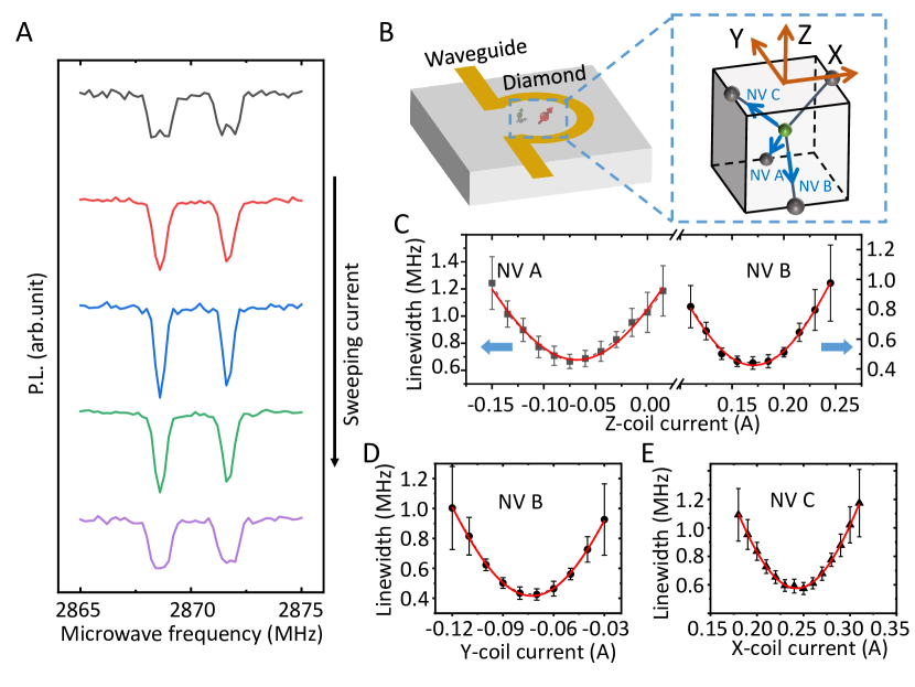
Figure S1: Schematics of the compensation process. (A) Variations of the ODMR spectra with sweeping currents applied to Helmholtz coils. (B) Orientations of four kinds of N-C bonds with respect to the lab frame. The blue arrows indicate the three differently orientated NV centers used for the magnetic-field compensation. (C)(D)(E) Compensation of $B_{z}$, $B_{y}$ and $B_{x}$, respectively. Series of ODMR spectra are measured with sweeping currents, and the linewidths are extracted with Gaussian fitting (not shown). The points are the fitting linewithds with error bars indicating the fitting error. To find the symmetric center points, a symmetric-peak function is used to fit the data. Here we choose Gaussian function for simplicity. The solid lines are fitting results.

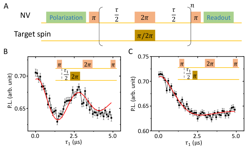
Figure S2: Zero-field DEER measurement. (A) The zero-field DEER sequence. The sequence is similar to the ordinary non-zero field case, but the $\pi/2$ and $\pi$ pulses are replaced by $\pi$ and $2\pi$ pulses, respectively. (B)(C) Comparison between two DEER measurements. The difference is flipping the target spin with $2\pi$ (A) or $\pi$ (B) RF pulse. Here $\tau=8$ $\mu$s. A faster evolution is observed by applying $2\pi$ RF pulse. The points are experimental results, while the lines are sine decay fitting. Error bars indicate s.e.m. Note here the ‘decay’ is actually a modulation, which is induced by multiple coupling strengths between the NV center and the P1 center, because of the fast jump of the P1 orientations.

Figure S3: Coherence properties of the NV center. The $T_{2}$ is measured by a similar sequence as the zero-field DEER, but without the manipulations on the target spin. The spin-locking decay is measured by applying a continuous driving field of the form $\Omega_{1}\cos{[Dt+2\Omega_{2}/\Omega_{1}\sin{\Omega_{1}t}]}$, where $D=2.87$ GHz, $\Omega_{1}=30$ MHz, and $\Omega_{2}=9$ MHz. In general, an oscillation with frequency of $\Omega_{1}$ can be observed according the calculations in Materials and Methods. Here we sample the data at integral periods, and thus only the envelope is presented. The points and lines are experimental and exponential fitting results, respectively. Error bars indicate s.e.m.

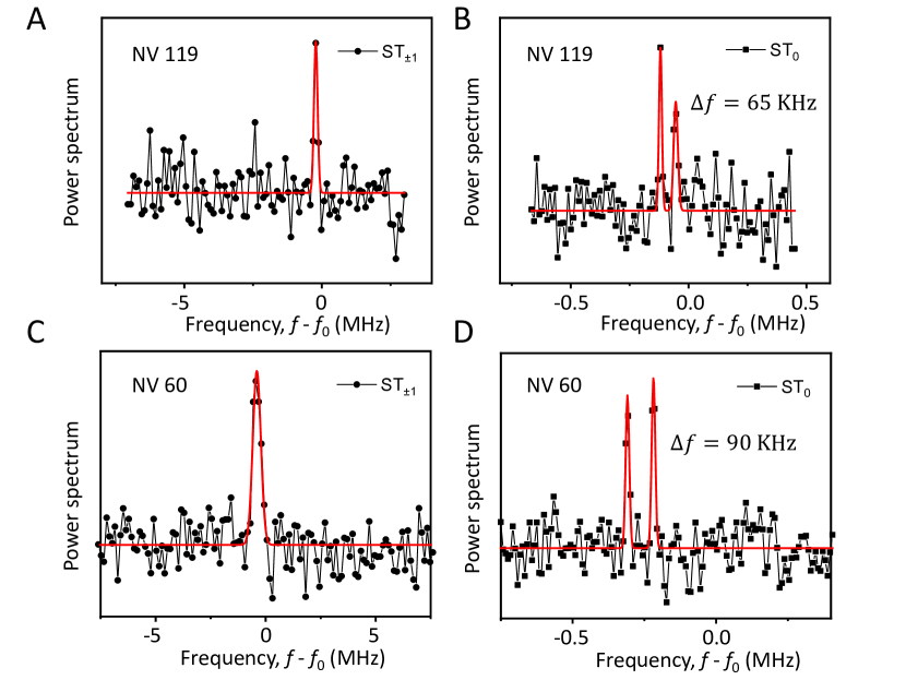
Figure S4: Zero-field EPR spectra of different P1 centers. (A)(C) $\text{ST}_{\pm 1}$ spectra. No obvious line splitting can be seen. (B)(D) $\text{ST}_{0}$ spectra. Clear line splitting can be seen with different splitting values. The data are measured on a ¹²C isotropically purified diamond, leading to the the disappearance of the line splitting in $\text{ST}_{\pm 1}$ spectra. However, the line splitting in $\text{ST}_{0}$ spectra remains, which rule out the reason of magnetic dipolar coupling with nearby nuclear spins. This splitting also differs for different P1 centers, suggesting different local electric or strain environments.

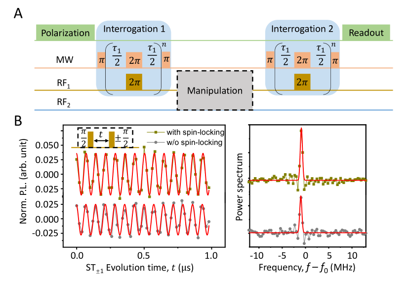
Figure S5: An alternative protocol for correlation detection. (A) The pulse sequence. Spin-locking sequence is replaced by two $\pi$ pulses. (B) Comparison between the two correlation detection protocol. The signal contrast of Ramsey experiment is partially lost without spin locking.

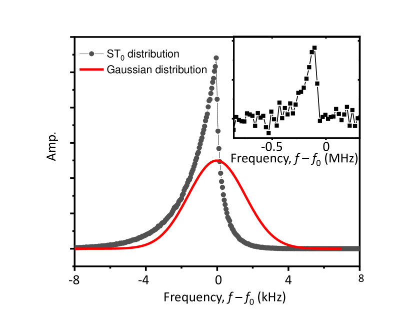
Figure S6: Simulation of the $\text{ST}_{0}$ spectrum. Black points are numerically calculated distribution of the $\text{ST}_{0}$ transition frequencies, while red line is a Gaussian distribution with the same standard deviation. Inset is the experimental spectrum with extra magnetic noise, generated by applying noise currents to the Helmholtz coils. This magnetic noise obeys the normal distribution with standard deviation of 2.3 MHz.