Exploring Spatial Significance via Hybrid Pyramidal Graph Network for Vehicle Re-identification

Abstract

Existing vehicle re-identification methods commonly use spatial pooling operations to aggregate feature maps extracted via off-the-shelf backbone networks. They ignore exploring the spatial significance of feature maps, eventually degrading the vehicle re-identification performance. In this paper, firstly, an innovative spatial graph network (SGN) is proposed to elaborately explore the spatial significance of feature maps. The SGN stacks multiple spatial graphs (SGs). Each SG assigns feature map’s elements as nodes and utilizes spatial neighborhood relationships to determine edges among nodes. During the SGN’s propagation, each node and its spatial neighbors on an SG are aggregated to the next SG. On the next SG, each aggregated node is re-weighted with a learnable parameter to find the significance at the corresponding location. Secondly, a novel pyramidal graph network (PGN) is designed to comprehensively explore the spatial significance of feature maps at multiple scales. The PGN organizes multiple SGNs in a pyramidal manner and makes each SGN handles feature maps of a specific scale. Finally, a hybrid pyramidal graph network (HPGN) is developed by embedding the PGN behind a ResNet-50 based backbone network. Extensive experiments on three large scale vehicle databases (i.e., VeRi776, VehicleID, and VeRi-Wild) demonstrate that the proposed HPGN is superior to state-of-the-art vehicle re-identification approaches.

I Introduction

Vehicle re-identification [1, 2] is a challenging yet meaningful computer vision task of retrieving vehicle images holding the same identity but captured from different surveillance cameras. Vehicles have different appearances at different spatial locations, which naturally causes feature maps containing varying spatial significance. Especially, subtle cues in local regions (e.g., lightings, stickers or pendants on windshields, and license plates) play critical roles in identifying highly similar vehicles of the same color and type/model. Therefore, exploring spatial significance of feature maps is crucial to improve vehicle re-identification performance.

In general, deep learning based vehicle re-identification models consist of backbone networks and feature aggregation architectures. Backbone networks take charge of learning three-dimensional (i.e., $height\times width\times channel$) feature maps from vehicle images. Feature aggregation architectures are responsible for aggregating the learned three-dimensional feature maps into feature vectors. Regarding backbone networks, a lot of off-the-shelf deep networks, such as VGGNet [3], GoogLeNet [4], ResNet [5, 6], DenseNet [7], and MobileNet [8], can be adopted. Based on those networks, backbone networks hold strong feature learning abilities. However, they still lack a special mechanism to explore the spatial significance of feature maps explicitly. One can design a new backbone network without using off-the-shelf deep networks to explore the spatial significance of feature maps. Nevertheless, it is challenging and daunting to design a new backbone network that can outperform off-the-shelf networks. Especially, those off-the-shelf deep networks have shown excellent advantages in many computer vision tasks. Therefore, how to explore the spatial significance of feature maps by feature aggregation architectures is received more and more research interests recently.

For aggregating feature maps extracted via backbone networks, many vehicle re-identification methods (e.g., [2, 9, 10, 11, 12, 13, 14, 15, 16, 17, 18, 19, 20, 21, 22]) use spatial global pooling operations. Although spatial global pooling operations are beneficial to learning viewpoint robust features, they only calculate feature maps’ spatial statistics (i.e., maximum or average), but ignore to explore the spatial significance of feature maps. To explore the spatial significance of feature maps, an alternative way is to divide vehicles into several parts and then features are learned on each part individually. Regarding part division ways, there are (1) uniform spatial divisions [23, 24, 25, 26, 27, 28], (2) spatial divisions [29, 30] using the spatial transformer network [31], (3) part detector based spatial divisions [32, 33, 34], and (4) key-point regressor based divisions [35, 10, 36, 37]. The first two kinds of spatial division methods are computationally economical but prone to suffer from part misalignments. In contrast, the last two kinds of spatial division methods could solve dis-alignments but encounter a high cost of extra manual part/key-point annotations and expensive training/inference computations. However, no matter how to divide parts, the subsequent feature learning is individually implemented on each part. As a result, the spatial significance of feature maps could not be jointly explored across multiple parts.

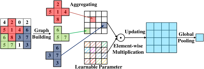
Figure 1: Exploring spatial significance before global pooling. For an easy visualization, single-channel feature maps are presented.

In this paper, to elaborately explore the spatial significance of feature maps extracted via a backbone network, an innovative spatial graph network (SGN) is designed. The SGN builds spatial graphs on the feature maps and re-weights feature maps’ elements at each spatial location via a learnable parameter before average pooling, as shown in Fig. 1. Furthermore, to comprehensively explore the spatial significance of feature maps at multiple scales, a novel pyramidal graph network (PGN) is designed to organize multiple SGNs and make each SGN deals with feature maps of a specific scale. As a result, a hybrid pyramidal graph network (HPGN) exploring spatial significance for vehicle re-identification is proposed by embedding the proposed PGN behind a ResNet-50 [5] based backbone network.

The main contributions of this paper are summarized in three folds. (1) An innovative spatial graph network (SGN) is designed to elaborately explore the spatial significance of feature maps resulted from a backbone network, without requiring any extra part division operations or part detectors/key-point regressors. To the best of our acknowledge, it is the first attempt to explore the spatial significance via graph networks. (2) A novel pyramidal graph network (PGN) is proposed to organize multiple SGNs to comprehensively explore the spatial significance of feature maps at multiple scales. (3) Extensive experiments on three large scale vehicle databases (i.e., VeRi776 [38], VehicleID [12], and VeRi-Wild [39]) show that the proposed method is superior to many state-of-the-art vehicle re-identification approaches.

The rest of this paper is organized as follows. Section II introduces the related work. Section III describes the proposed method. Section IV presents experiments and analyses to validate the proposed method’s superiority. Section V concludes this paper.

II Related Work

II-A Vehicle Re-identifications

Given a backbone network based on off-the-shelf backbone networks (e.g., VGGNet [3], GoogLeNet [4], ResNet [5, 6], DenseNet [7], and MobileNet [8]), vehicle re-identification progress is reviewed from two aspects: (1) feature aggregation architectures and (2) loss functions.

II-A1 Feature Aggregation Architectures

There are two types of feature aggregation architectures: (1) the global-level feature aggregation architecture and (2) the part-level feature aggregation architecture. The global-level aggregation architecture usually is a spatial global pooling layer, as done in [2, 9, 10, 11, 12, 13, 14, 15, 16, 17, 18, 19, 20, 21, 22]. Spatial global pooling layers are non-parameterized, which find the maximal or average spatial statistic on each channel of feature maps extracted via a backbone network. Using spatial global pooling layers, there is an advantage of learning viewpoint robust features. However, due to the characteristic of spatial global pooling layers, the varying spatial significance of feature maps will be inevitably ignored, which is detrimental to vehicle re-identification.

According to the way of dividing vehicle parts, there are two kinds of part-level feature aggregation architectures: (1) part annotation free feature aggregation architectures and (2) part annotation required feature aggregation architectures. Regarding part annotation free feature aggregation architectures, the most straightforward and economical method is the uniform spatial division pooling strategy, which equally divides feature maps into several parts and pools each part individually, as done in [23, 24, 25]. Since parts are divided rigidly, the uniform spatial division pooling strategy is prone to suffering from part dis-alignments. To alleviate dis-alignments, [26, 27, 28] simultaneously apply spatial global and spatial division pooling strategies, and [29, 30] use the spatial transformer network [31] to determine part regions. Besides, in [28, 29, 30], visual attention modules(e.g., the self-attention [40] and the residual attention [41]) are adopted for refining features on each part. Nevertheless, part dis-alignments are still serious since lacking accurate part detectors.

Regarding part annotation required feature aggregation architectures, in [32, 33, 34], typical detectors, such as the faster region-based convolutional neural network (Faster R-CNN) [42], the you only look once (YOLO) model [43], and the single shot multi-box detector (SSD) [44], are applied to detect vehicle parts, e.g., lightings, front windshields, and logos. Additionally, in [35, 10, 36, 37], key-point regressors are employed to locate informative vehicle regions. However, both typical detectors and key-point regressors are deep networks in themselves, along with a high cost of extra manual part annotations or key-point annotations and expensive training/inference computations.

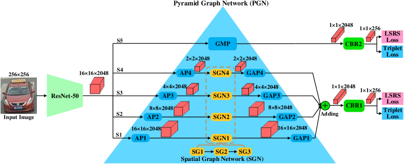
Figure 2: The framework of the proposed hybrid pyramidal graph network (HPGN). Here, AP denotes an average pooling layer; GAP and GMP respectively represent a global average pooling layer and a global max pooling layer; CBR represents a composite unit that consists of a convolutional layer using $1\times 1$ sized filters, a batch normalization layer [45] and a rectified linear unit (ReLU) [46]; LSRS means that the label smoothing regularized softmax loss [47].

II-A2 Loss Functions

Many vehicle re-identification methods (e.g., [18, 11, 12, 13, 30]) show promising performance by combining softmax [48, 47] and triplet loss [49, 11] functions. Because the softmax loss is beneficial to the convergence speed, and the triplet loss is helpful to learn discriminative features. In addition to contaminating softmax [48] and triplet [11] loss functions, sample mining strategies (e.g., hard negative/positive sample mining) also can improve vehicle re-identification [18]. Besides, there are some variant triplet loss functions [11, 12, 50, 51, 52, 15] for vehicle re-identification. For example, the group-group (GGL) loss function [50] computes the loss on image groups rather than image pairs or triplets, simplifying the model training process. The group sensitive triplet embedding (GSTE) method [51] improves the triplet loss function by well dealing with the intra-class variance. The multi-view ranking loss (MRL) [52] approach divides the triplet loss into a single-view ranking loss and a cross-view ranking loss to appropriately handle viewpoint variations.

II-B Graph Convolutional Network

The graph convolutional network (GCN) [53, 54, 55] initially is for learning features on non-Euclidean data, which can flexibly aggregate nodes to learn features. Recent studies show that GCN has high potentials in many computer vision tasks, such as multi-label recognition [56], action recognition [57, 58, 59], and person re-identification [60, 61, 62, 63, 64]. Especially, with the strength of GCN, a similar task to this paper, i.e., person re-identification, receives a list of advantages, such as the refining of the similarity between an image pair [60], the robustness to individuals’ appearance and membership changes [61], and the robustness to noise of initial training data [63].

Regarding the graph construction way, all those GCN based person re-identification methods [60, 61, 62, 63, 64] build a graph involving multiple individuals where an individual person is assigned as a node. In contrast, this paper independently constructs a graph for each individual. More specifically, this paper develops a graph network on feature maps of a vehicle individual to elaborately explore the spatial significance. In the proposed graph network, each element of a feature map is assigned as a node, and a parameter is learned for re-weighting each node to explore the spatial significance of feature maps.

III Proposed Method

III-A Overview

As shown in Fig. 2, the proposed hybrid pyramidal graph network (HPGN) is mainly constructed by embedding a pyramidal graph network (PGN) following a ResNet-50 based backbone network. Regarding the PGN, it is composed of multiple spatial graph networks (SGNs). Each SGN stacks three spatial graphs (SGs) to handle a feature map of a specific scale. Each SG assigns feature map’s elements as nodes and utilizes spatial neighborhood relationships to determine edges among nodes. Each node and its spatial neighbors on an SG are aggregated to the next SG during the SGN’s propagation. Then, each aggregated node of the next SG is re-weighted with a learnable parameter to automatically find the significance at the corresponding location. Regarding the backbone network, the ResNet-50 [5] is applied, which is commonly used in previous re-identification works [65, 66, 67, 32, 10]. Besides, following [65], the ‘last stride=1’ training trick is applied to set the last stride of the fourth residual layer to 1. Consequently, for a $256\times 256$ sized input vehicle image, the ResNet-50 extracts a $16\times 16\times 2048$ sized feature map that will be further handled with the PGN and loss functions. More detail about the PGN and loss functions are described as follows.

III-B Pyramidal Graph Network

The PGN contains two essential designs, namely, the spatial graph network (SGN) and the pyramidal architecture (PA). The SGN is designed to explore the spatial significance of feature maps at one scale. The PA is designed to organize multiple SGNs to comprehensively explore spatial significance of feature maps at multiple scales. The detail of SGN and PA are introduced as follows.

III-B1 Spatial Graph Network

Assume that $X\in R^{h\times w\times c}$ is a three-dimensional feature map extracted by using the backbone network (i.e., ResNet-50 [5]), where $h$, $w$, and $c$ represents height, width, and channel number of $X$. For ease of description, $X$ is reshaped as a matrix $V\in R^{d\times c}$ by rearranging each channel of $X$ into a $d$ dimensional vector, where $d=h\times w$. Then, a spatial graph $G=\{V\in R^{d\times c},E\in R^{d\times d\times c}\}$ assigns each element of the vector $V$ as a node. Furthermore, the spatial graph’s edges are constructed according to Eq. (1), as follows.

$$E_{i,j,k}=\left\{\begin{array}[]{cc}\frac{1}{|N_{V_{i,k}}|},&V_{j,k}\in N_{V_{i,k}},\\ 0,&{otherwise},\end{array}\right.$$ (1)

where $i,j\in[1,2,...,d]$ and $k\in[1,2,...,c]$; $E_{i,j,k}$ is the edge between the node $V_{i,k}$ and the node $V_{j,k}$ on the $k$-th channel; $N_{V_{i,k}}$ represents the neighbor node set of $V_{i,k}$, and $|N_{V_{i,k}}|$ denotes the number of nodes in $N_{V_{i,k}}$.

In order to simplify the edge definition of Eq. (1), the edge definition on each channel is assumed to be identical. Specifically, $N_{V_{i,k}}$ is determined according to the four spatial neighbors (i.e., up, down, left, and right) of node $V_{i,k}$. Moreover, if $V_{i,k}$ is a boundary node, its neighbors are reduced according to its actual location since zero-padding operations are given up in this paper. As a result, the edge definition of Eq. (1) is simplified as follows:

$$\begin{array}[]{cc}{E_{i,j,1}}={E_{i,j,2}}=...={E_{i,j,c}}={S_{i,j}},\\ {S_{i,j}}=\left\{{\begin{array}[]{*{20}{c}}{\frac{1}{{|{N_{{V_{i,1}}}}|}},}&{{V_{j,1}}\in{N_{{V_{i,1}}}},}\\ {0,}&{otherwise.}\end{array}}\right.\\ \end{array}$$ (2)

Based on the simplified edge definition of Eq. (2), the spatial graph $G=\{V\in R^{d\times c},S\in R^{d\times d}\}$ is built, and the node aggregation is according to Eq. (3), as follows.

$$A=IV+SV=\left(I+S\right)V,$$ (3)

where $I=diag(1,1,1,...,1)\in R^{d\times d}$ is an identity matrix; $A\in R^{d\times c}$ is a matrix containing aggregated nodes. Then, each aggregated node is further updated by using Eq. (4), as follows:

$$U=A\odot{\varTheta},$$ (4)

where $\odot$ represents an element-wise multiplication operation; $\varTheta\in R^{d\times c}$ is a learnable parameter matrix used to explore the spatial significance via re-weighting aggregated nodes of $A$. Consequently, $U$ can take the varying spatial significance of feature maps into account.

From Eq. (3) and Eq. (4), one can see that both a node itself and its neighbor nodes are aggregated to feed more information for exploring the significance at the corresponding location. Besides, regarding Eq. (4), different from existing works [60, 61] that use a multi-layer perceptron (MLP) to update aggregated nodes, the proposed method applies an element-wise multiplication operation. Because the goal of proposed method is to explore the spatial significance rather than to transform features complexly.

Both Eq. (3) and Eq. (4) are linear calculations. In order to introduce non-linearities and improve the spatial graph’s convergence, Eq. (4) is enhanced as follows:

$$O=LeakyReLU\left(BN\left(U\right)\right),$$ (5)

where $LeakyReLU$ represents the leaky rectified linear unit [68] of a 0.2 slope parameter; $BN$ denotes the batch normalization [45]; $O\in R^{d\times c}$ replaces $U$ as the new feature map that non-linearly deals with the spatial significance. Finally, according to Eq. (2), Eq. (3), Eq. (4), and Eq. (5), a spatial graph (SG) can be built, and then the spatial graph network (SGN) is constructed by stacking multiple spatial graphs (SGs).

III-B2 Pyramidal Architecture

As shown in Fig. 2, a pyramidal architecture containing multiple SGNs is further designed to comprehensively explore the spatial significance of feature maps at multiple scales. First, for a $16\times 16\times 2048$ sized feature map extracted by the ResNet-50 [5] based backbone network, five pooling layers (i.e., AP1, AP2, AP3, AP4, and GMP) are simultaneously applied to resize the feature map to acquire multi-scale feature maps, i.e., $16\times 16\times 2048$, $8\times 8\times 2048$, $4\times 4\times 2048$, $2\times 2\times 2048$, and $1\times 1\times 2048$ sized feature maps. The configurations of these five pooling layers are listed in Table I. Please note that the AP1 layer is just for the elegant presentation of Fig. 2. In practice, the AP1 layer can be removed since performing an $1\times 1$ sized average pooling operation on a feature map does not change the feature map.

Second, following AP1, AP2, AP3, and AP4 layers, four spatial graph networks (i.e., SGN1, SGN2, SGN3, and SGN4) are applied to explore the spatial significance of $16\times 16\times 2048$, $8\times 8\times 2048$, $4\times 4\times 2048$, $2\times 2\times 2048$ sized feature maps, respectively. Moreover, on the minimal sized (i.e., $1\times 1\times 2048$) feature map, there is no spatial graph network since the $1\times 1$ resolution is too small.

Third, following SGN1, SGN2, SGN3, and SGN4, four global average pooling (i.e., GAP1, GAP2, GAP3, and GAP4) are respectively employed to aggregate feature maps. The configurations of GAP1, GAP2, GAP3, and GAP4 are also listed in Table I. In our implementation, to reduce model complexities, these four spatial graph networks (SGNs) hold the same architecture, i.e., each SGN has three spatial graphs, as shown in Fig. 2.

TABLE I: The configuration of pooling layers in the proposed PGN.

Components	Pooling Window ($height\times width$)	Channels	Stride	Padding
AP1	$1\times 1$	2048	1	0
AP2	$2\times 2$	2048	2	0
AP3	$4\times 4$	2048	4	0
AP4	$8\times 8$	2048	8	0
GMP	$16\times 16$	2048	1	0
GAP1	$16\times 16$	2048	1	0
GAP2	$8\times 8$	2048	1	0
GAP3	$4\times 4$	2048	1	0
GAP4	$2\times 2$	2048	1	0

III-C Loss Function Design

From Fig. 2, one can see that the proposed PGN applies a global max pooling (GMP) layer to produce the minimal sized (i.e., $1\times 1\times 2048$) feature map, while uses average pooling layers (i.e., GAP1, GAP2, GAP3, and GAP4) to generate larger sized feature maps. This configuration of using two kinds of pooling layers are beneficial to enrich multi-scale feature maps. Based on this configuration, two sets of loss functions are assigned to supervise features resulted from max and average pooling layers. More details are described as follows.

Firstly, an adding layer is utilized to accumulate features produced by GAP1, GAP2, GAP3, and GAP4. Secondly, two CBR composite units (i.e., CBR1 and CBR2) are embedded after the adding layer and the GMP layer individually to reduce the feature dimension from 2048 to 256. The CBR composite unit is composed of a convolutional layer using $1\times 1$ sized filters, a batch normalization [45] layer, and a rectified linear unit (ReLU) [46]. Finally, on CBR1 and CBR2, the proposed HPGN’s total loss function is formulated as follows:

$${L_{total}}=\alpha L_{lsrs}^{CBR1}+\beta L_{triplet}^{CBR1}+\rho L_{lsrs}^{CBR2}+\lambda L_{triplet}^{CBR2},$$ (6)

where $L_{lsrs}^{CBR1}$ and $L_{lsrs}^{CBR2}$ are label smoothing regularized softmax (LSRS) loss functions [47] playing on CBR1 and CBR2, respectively; similarly, $L_{triplet}^{CBR1}$ and $L_{triplet}^{CBR2}$ are the triplet loss functions [69] working on CBR1 and CBR2, respectively; $\alpha$, $\beta$, $\rho$, and $\lambda\geq 0$ are manually setting constants used to keep the balance of four loss functions. To avoid excessive tuning those constants, we set $\alpha=\rho=2$ and $\beta=\lambda=1$ in the following experiments. The LSRS loss function [47] is formulated as follows:

$${{L_{lsrs}}(X,l)=\frac{{-1}}{M}\sum\limits_{i=1}^{M}{\sum\limits_{j=1}^{K}{\delta({l_{i}},j)log(\frac{{{e^{W_{j}^{\rm{T}}{X_{i}}}}}}{{\sum\nolimits_{k=1}^{K}{{e^{W_{k}^{\rm{T}}{X_{i}}}}}}})}},}$$ (7)

$${\delta({l_{i}},j)=\left\{\begin{array}[]{cc}1-\varepsilon+\frac{\varepsilon}{K},&j={l_{i}},\\ \frac{\varepsilon}{K},&{otherwise},\end{array}\right.}$$ (8)

where $X$ is a training set and $l$ is the class label information; $M$ is the number of training samples; $K$ is the number of classes; $(X_{i},l_{i})$ is the $i$-th training sample and $l_{i}\in\{1,2,3,...,K\}$; $W=[W_{1},W_{2},W_{3},...,W_{K}]$ is a learnable parameter matrix; $\varepsilon\in[0,1)$ is a tiny constant used to control the smoothing regularization degree, which is set to $0.1$ in this paper, as done in [47].

The triplet loss function [69] is formulated as follows:

$${L_{triplet}}({X^{a}},{X^{n}},{X^{p}})$$ (9)

$$= \frac{{-1}}{M}\sum\limits_{i=1}^{M}{\max({{\left\|{X_{i}^{a}-X_{i}^{n}}\right\|}_{2}}-{{\left\|{X_{i}^{a}-X_{i}^{p}}\right\|}_{2}}-\tau,0)},$$

where $({X^{a}},{X^{n}},{X^{p}})$ is a set of training triplets; $M$ is the number of training triplets; for the $i$-th training triplet, $(X^{a}_{i},X^{n}_{i})$ is a negative pair of different class labels, and $(X^{a}_{i},X^{p}_{i})$ is a positive pair of the same class label; $\tau\geq 0$ is a margin constant, which is set to $1.2$ in following experiments; $\left\|\cdot\right\|_{2}$ denotes the Euclidean distance. Besides, the hard sample exploring strategy [69] is applied to improve the triplet loss, aiming to find the most difficult positive and negative image pairs in each mini-batch.

IV Experiment and Analysis

To validate the superiority of the proposed hybrid pyramidal graph network (HPGN) method, it is compared with state-of-the-art vehicle re-identification approaches on three large-scale databases. The rank-1 identification rate (R1) and mean average precision (mAP) are used as performance metrics.

IV-A Databases

VeRi776 [38] is collected by 20 cameras in unconstrained traffic scenarios, and each vehicle is captured by 2-18 cameras. Following the evaluation protocol of [38], VeRi776 is separated into a training subset and a testing subset. The training subset contains 37,746 images of 576 subjects. The testing subset includes a probe subset of 1,678 images of 200 subjects and a gallery subset of 11,579 images of the same 200 subjects. Besides, only cross-camera vehicle pairs are evaluated, which means that if a probe image and a gallery image are captured by the same camera, the corresponding result will be excluded in the evaluation process.

VehicleID [12] includes 221,763 images of 26,267 subjects. Each vehicle is captured from either front or rear viewpoint. The training subset consists of 110,178 images of 13,164 subjects. There are three testing subsets, i.e., Test800, Test1600, and Test2400, for evaluating the performance at different data scales. Specifically, Test800 includes 800 gallery images and 6,532 probe images of 800 subjects. Test1600 contains 1,600 gallery images and 11,395 probe images of 1,600 subjects. Test2400 consists of 2,400 gallery images and 17,638 probe images of 2,400 subjects. Besides, for three testing subsets, the division of probe and gallery subsets is as follows: randomly selecting one image of a subject to form the probe subset, and the subject’s remaining images are used to construct the gallery subset. This division is repeated and evaluated ten times, and the average result is reported as the final performance.

VERI-Wild [39] is a newly dataset released in CVPR 2019. Different to VeRi776 [38] and VehicleID [12] captured at day, VERI-Wild are captured at both day and night. The training subset of 277,797 images of 30,671. Besides, as in VehicleID [12], there are three different scale testing subsets, i.e., Test3000, Test5000, and Test10000. Test3000 has 41,816 gallery images and 3000 probe images of 3,000 subjects. Test5000 contains 69,389 gallery images and 5,000 probe images of 5,000 subjects. Test10000 includes 138,517 gallery images and 10,000 probe images of 10,000 subjects.

IV-B Implementation Details

The deep learning toolbox is Pytorch [70]. Training configurations are summarized as follows. (1) Random erasing [71], horizontal flip, and z-score normalization are used for the data augmentation. For both horizontal flip and random erasing operations, the implementation probability is set to 0.5. (2) The mini-batch stochastic gradient descent (SGD) method [72] is applied to optimize parameters. The weight decays are set to 5$\times$10^-4, and the momentums are set to 0.9. There are 150 epochs for the training process. The learning rates are initialized to 3$\times$10^-4, and they are linearly warmed up [65] to 3$\times$10^-2 in the first 10 epochs. After warming up, the learning rates are maintained at 3$\times$10^-2 from 11th to 50th epochs. Then, the learning rates are reduced to 3$\times$10^-3 from 51st to 85th epochs. Furthermore, the learning rates are decayed to 3$\times$10^-4 after 85 epochs, and they are reduced to 3$\times$10^-5 from 120th and 150th epochs. (3) Each mini-batch includes 32 subjects, and each subject holds 4 images. During the testing phase, those 256-dimensional features resulted from CBR1 and CBR2 (see Fig. 2) are concatenated as final features of vehicle images. Moreover, the Cosine distance of final features is applied as the similarity measurement for vehicle re-identification.

IV-C Comparison with State-of-the-art Methods

TABLE II: The performance (%) comparison on VeRi776. The red, green and blue rows respectively represent the $1$st, $2$nd and $3$rd places, according to the R1 comparison.

Methods	R1	mAP	References
HPGN	96.72	80.18	Proposed
QD-DLF [24]	88.50	61.83	IEEE ITS 2020
Appearance+License [73]	95.41	78.08	ICIP 2019
SFF+SAtt [28]	94.93	74.11	IJCNN 2019
Part Regularization [32]	94.30	74.30	CVPR 2019
SAN [27]	93.30	72.50	arXiv 2019
PAMTRI [37]	92.86	71.88	ICCV2019
MLFN+Triplet [74]	92.55	71.78	CVPRW 2019
MTML+OSG+Re-ranking [75]	92.00	68.30	CVPRW 2019
MRM [76]	91.77	68.55	Neurocomputing 2019
DMML [77]	91.20	70.10	ICCV 2019
Triplet Embedding [18]	90.23	67.55	IJCNN 2019
MOV1+BS [78]	90.20	67.60	CVPR 2019
VANet [15]	89.78	66.34	ICCV 2019
GRF+GGL [50]	89.40	61.70	IEEE TIP 2019
ResNet101-AAVER [10]	88.97	61.18	ICCV 2019
MRL [52]	87.70	71.40	ICME 2019
Fusion-Net [79]	87.31	62.40	IEEE TIP 2019
Mob.VFL-LSTM [80]	87.18	58.08	ICIP 2019
MGL [66]	86.10	65.00	ICIP 2019
EALN [21]	84.39	57.44	IEEE TIP 2019
FDA-Net [39]	49.43	N/A	CVPR 2019
JDRN+Re-ranking [81]	N/A	73.10	CVPRW 2019
MAD+STR [14]	89.27	61.11	ICIP 2018
RAM [26]	88.60	61.50	ICME 2018
VAMI [82]	85.92	61.32	CVPR 2018
GSTE [51]	N/A	59.47	IEEE TMM 2018
SDC-CNN [83]	83.49	53.45	ICPR 2018
PROVID [2]	81.56	53.42	IEEE TMM 2018
NuFACT+Plate-SNN [2]	81.11	50.87	IEEE TMM 2018
SCCN-Ft+CLBL-8-Ft [84]	60.83	25.12	IEEE TIP 2018
ABLN-Ft-16 [85]	60.49	24.92	WACV 2018
NuFACT [2]	76.76	48.47	IEEE TMM 2018
VST Path Proposals [16]	83.49	58.27	ICCV 2017
OIFE+ST [35]	68.30	51.42	ICCV 2017
DenseNet121 [7]	80.27	45.06	CVPR 2017
FACT [1]	52.21	18.75	ICME 2016
VGG-CNN-M-1024 [12]	44.10	12.76	CVPR 2016
GoogLeNet [86]	52.32	17.89	CVPR 2016

TABLE III: The performance (%) comparison on VehicleID. The red, green and blue rows respectively represent the $1$st, $2$nd and $3$rd places, according to R1 comparison.

Methods	Test800		Test1600		Test2400		References
	R1	mAP	R1	mAP	R1	mAP
HPGN	83.91	89.60	79.97	86.16	77.32	83.60	Proposed
QD-DLF [24]	72.32	76.54	70.66	74.63	64.14	68.41	IEEE ITS 2020
Appearance+License [73]	79.5	82.7	76.9	79.9	74.8	77.7	ICIP 2019
MGL [66]	79.6	82.1	76.2	79.6	73.0	75.5	ICIP 2019
Part Regularization [32]	78.40	N/A	75.00	N/A	74.20	N/A	CVPR 2019
PRN[23]	78.92	N/A	74.94	N/A	71.58	N/A	CVPRW 2019
Triplet Embedding [18]	78.80	86.19	73.41	81.69	69.33	78.16	IJCNN 2019
MRM [76]	76.64	80.02	74.20	77.32	70.86	74.02	Neurocomputing 2019
XG-6-sub-multi [87]	76.1	N/A	73.1	N/A	71.2	N/A	IEEE ITS 2019
GRF+GGL [50]	77.1	N/A	72.7	N/A	70.0	N/A	IEEE TIP 2019
MSV [20]	75.1	79.3	71.8	75.4	68.7	73.3	ICASSP 2019
DQAL [88]	74.74	N/A	71.01	N/A	68.23	N/A	IEEE TVT 2019
EALN [21]	75.11	77.5	71.78	74.2	69.30	71.0	IEEE TIP 2019
Mob.VFL-LSTM [80]	73.37	N/A	69.52	N/A	67.41	N/A	ICIP 2019
ResNet101-AAVER [10]	74.69	N/A	68.62	N/A	63.54	N/A	ICCV 2019
TAMR [30]	66.02	N/A	62.90	N/A	59.69	N/A	IEEE TIP 2019
MLSR [89]	65.78	N/A	64.24	N/A	60.05	N/A	Neurocomputing 2019
RPM [29]	65.04	N/A	62.55	N/A	60.21	N/A	ICMEW 2019
SFF+SAtt [28]	64.50	N/A	59.12	N/A	54.41	N/A	IJCNN 2019
FDA-Net [39]	N/A	N/A	59.84	65.33	55.53	61.84	CVPR 2019
GSTE [51]	75.90	75.40	74.80	74.30	74.00	72.40	IEEE TMM 2018
RAM [26]	75.20	N/A	72.3	N/A	67.70	N/A	ICME 2018
C2F [17]	61.10	63.50	56.20	60.00	51.40	53.00	AAAI 2018
VAMI [82]	63.12	N/A	52.87	N/A	47.34	N/A	CVPR 2018
SDC-CNN [83]	56.98	63.52	50.57	57.07	42.92	49.68	ICPR 2018
NuFACT [2]	48.90	N/A	43.64	N/A	38.63	N/A	IEEE TMM 2018
MAD+STR [14]	N/A	82.20	N/A	75.90	N/A	72.80	ICIP 2018
PMSM [34]	N/A	64.20	N/A	57.20	N/A	51.80	ICPR 2018
MSVF [19]	N/A	N/A	N/A	N/A	46.61	N/A	GCPR 2018
ABLN-32 [85]	52.63	N/A	N/A	N/A	N/A	N/A	WACV 2018
DJDL [13]	72.30	N/A	70.80	N/A	68.00	N/A	ICIP 2017
Improved Triplet [11]	69.90	N/A	66.20	N/A	63.20	N/A	ICME 2017
DenseNet121 [7]	66.10	68.85	67.39	69.45	63.07	65.37	CVPR 2017
MGR[9]	N/A	62.80	N/A	62.30	N/A	61.23	ICCV 2017
OIFE+ST [35]	N/A	N/A	N/A	N/A	67.00	N/A	ICCV 2017
DRDL [12]	48.91	N/A	46.36	N/A	40.97	N/A	CVPR 2016
FACT [1]	49.53	N/A	44.63	N/A	39.91	N/A	ICME 2016

IV-C1 Comparisons on VeRi776

From Table II, it can be found that the vehicle re-identification performance has made significant progress between 2016 and 2020 on VeRi776 [38]. Especially in 2019, many approaches [73, 28, 32, 37, 74, 75, 76, 77, 18, 78] acquire more than 90% rank-1 identification rates. Under this background, the proposed HPGN method achieves the highest rank-1 identification rate (i.e., 96.72%) and the largest mAP (i.e., 80.18%). For example, among those compared state-of-the-art methods, rank-1 identification rates of the 2nd place (i.e., Appearance+License [73]) and the 3rd place (i.e., SFF+SAtt+TBR [28]) are 1.31% and 1.79% lower than those of HPGN, respectively. Besides, regarding mAP performance, Appearance+License [73] and SFF+SAtt+TBR [28] are 2.10% and 6.07% lower than that of HPGN, respectively. It is worth mentioning that both Appearance+License [73] and SFF+SAtt+TBR [28] use the same backbone network (i.e., ResNet-50 [5]) to HPGN. However, HPGN does not require vehicle attribute aids, e.g., license plates and temporal Bayesian re-rankings (TBR).

IV-C2 Comparisons on VehicleID

Table III shows the comparison of the proposed HPGN method and state-of-the-art approaches on VehicleID [12] that has a larger data scale than VeRi776 [38]. One can see that many approaches (e.g., [73, 66, 32, 18, 23, 76, 87, 50, 20, 88, 21]) made significant progress in 2019 on VehicleID, but HPGN outperforms all of them. More specifically, Appearance+License [73] still is the 2nd place and in superior to HPGN. For example, the R1 and mAP of Appearance+License [73] are 4.41% and 6.90% lower than those of HPGN on Test800, respectively. Regarding the 3rd place, without the help of temporal Bayesian re-ranking (TBR), the performance rank of SFF+SAtt [28] drops dramatically. MGL [66] replaces SFF+SAtt [28] as the 3rd place, and its R1 and mAP are 4.31% and 7.50% lower than those of HPGN on Test800, respectively. In summary, although Appearance+License [73], SFF+SAtt [28], MGL [66], and HPGN adopt the same backbone network (i.e., ResNet-50 [5]), HPGN acquires the 1st place on both VehicleID [12] and VeRi776 [38], which solidly demonstrates the HPGN’s superiority.

IV-C3 Comparisons on VeRi-Wild

Table IV shows the comparison result on VeRi-Wild [39]. Since VeRi-Wild [39] is a newly released dataset, only a few methods have been evaluated on it. Among those methods, it can be found that the proposed HPGN method obtains the 1st place again. For example, HPGN outperforms the 2nd place, namely, Triplet Embedding [18], by a 12.69% higher rank-1 identification rate on Test10000.

TABLE IV: The performance (%) comparison on VERI-Wild. The red, green and blue rows respectively represent the $1$st, $2$nd and $3$rd places, according to the R1 comparison.

Methods	Test3000		Test5000		Test10000		References
	R1	mAP	R1	mAP	R1	mAP
HPGN	91.37	80.42	88.21	75.17	82.68	65.04	Proposed
Triplet Embedding [18]	84.17	70.54	78.22	62.83	69.99	51.63	IJCNN 2019
FDA-Net [39]	64.03	35.11	57.82	29.80	49.43	22.80	CVPR 2019
GSTE [51]	60.46	31.42	52.12	26.18	45.36	19.50	IEEE TMM 2018
Unlabled GAN [90]	58.06	29.86	51.58	24.71	43.63	18.23	ICCV 2017
GoogLeNet [4]	57.16	24.27	53.16	24.15	44.61	21.53	CVPR 2015
HDC [91]	57.10	29.14	49.64	24.76	43.97	18.30	ICCV 2017
DRDL [12]	56.96	22.50	51.92	19.28	44.60	14.81	CVPR 2016
Softmax [38]	53.40	26.41	46.16	22.66	37.94	17.62	ECCV 2016
Triplet [49]	44.67	15.69	40.34	13.34	33.46	9.93	CVPR 2015

IV-D Analysis

The comparison results presented in Tables II, III, and IV demonstrate that the proposed HPGN method is superior to a lot of state-of-the-art vehicle re-identification methods. In what follows, the proposed HPGN method is comprehensively analyzed from four aspects to investigate the logic behind its superiority. (1) The role of pyramidal graph network (PGN). (2) The influence of changing depths of spatial graph networks (SGNs). (3) The impact of varying HPGN’s scale configurations. (4) The spatial significance visualization.

TABLE V: The role (%) of pyramidal graph network (PGN).

Methods	VeRi776		VehicleID						VERI-Wild
			Test800		Test1600		Test2400		Test3000		Test5000		Test10000
	R1	mAP	R1	mAP	R1	mAP	R1	mAP	R1	mAP	R1	mAP	R1	mAP
HPGN	96.72	80.18	83.91	89.60	79.97	86.16	77.32	83.60	91.37	80.42	88.21	75.17	82.68	65.04
HPGNOI	96.06	78.87	82.45	88.85	78.62	85.28	75.88	82.55	90.11	78.22	86.03	74.31	79.91	63.27
HPGNNG	95.23	75.90	82.02	87.87	78.04	84.08	75.23	81.65	88.67	76.34	85.84	72.48	78.32	61.22
Baseline	94.12	74.65	79.48	86.13	75.81	82.21	72.80	79.54	88.18	72.16	83.95	65.08	76.82	55.60

TABLE VI: The performance (%) comparison among those hybrid pyramidal graph networks (HPGNs) holding pyramidal graph networks (PGNs) of different scale configurations.

Names	Scales	VeRi776		VehicleID						VERI-Wild
				Test800		Test1600		Test2400		Test3000		Test5000		Test10000
		R1	mAP	R1	mAP	R1	mAP	R1	mAP	R1	mAP	R1	mAP	R1	mAP
Baseline	S5	94.12	74.65	79.48	86.13	75.81	82.21	72.80	79.54	88.18	72.16	83.95	65.08	76.82	55.60
HPGN1	S5, S4	95.65	78.91	81.82	87.93	77.49	83.96	74.56	81.12	89.43	76.52	86.07	72.42	79.37	61.25
HPGN2	S5, S4, S3	95.95	79.03	82.92	88.75	79.18	85.40	75.96	82.47	89.71	77.34	86.82	73.88	79.96	62.45
HPGN3	S5, S4, S3, S2	96.06	79.35	83.58	89.16	79.33	85.54	76.05	82.57	90.66	78.84	87.13	74.09	80.24	63.88
HPGN	S5, S4, S3, S2, S1	96.72	80.18	83.91	89.60	79.97	86.16	77.32	83.60	91.37	80.42	88.21	75.17	82.68	65.04

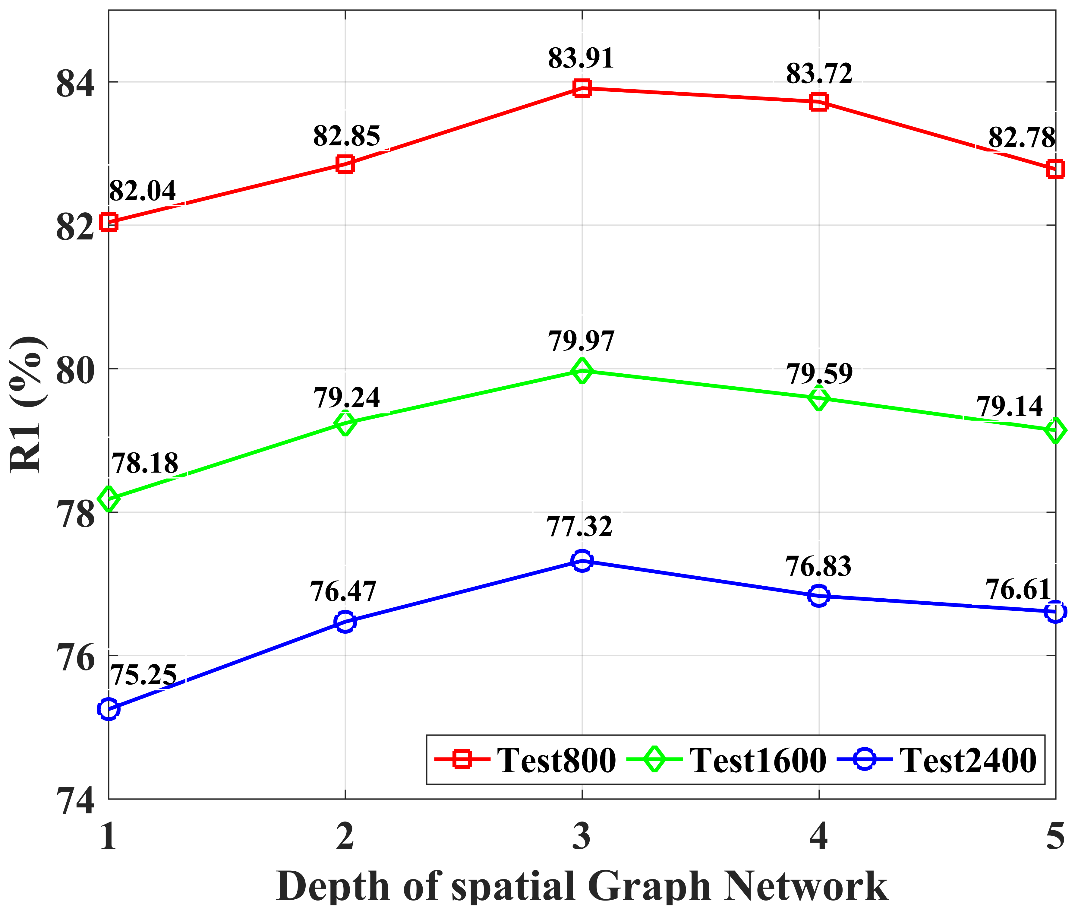
Figure 3: The rank-1 identification rate (R1) comparison among spatial graph networks of different depth on VehicleID.

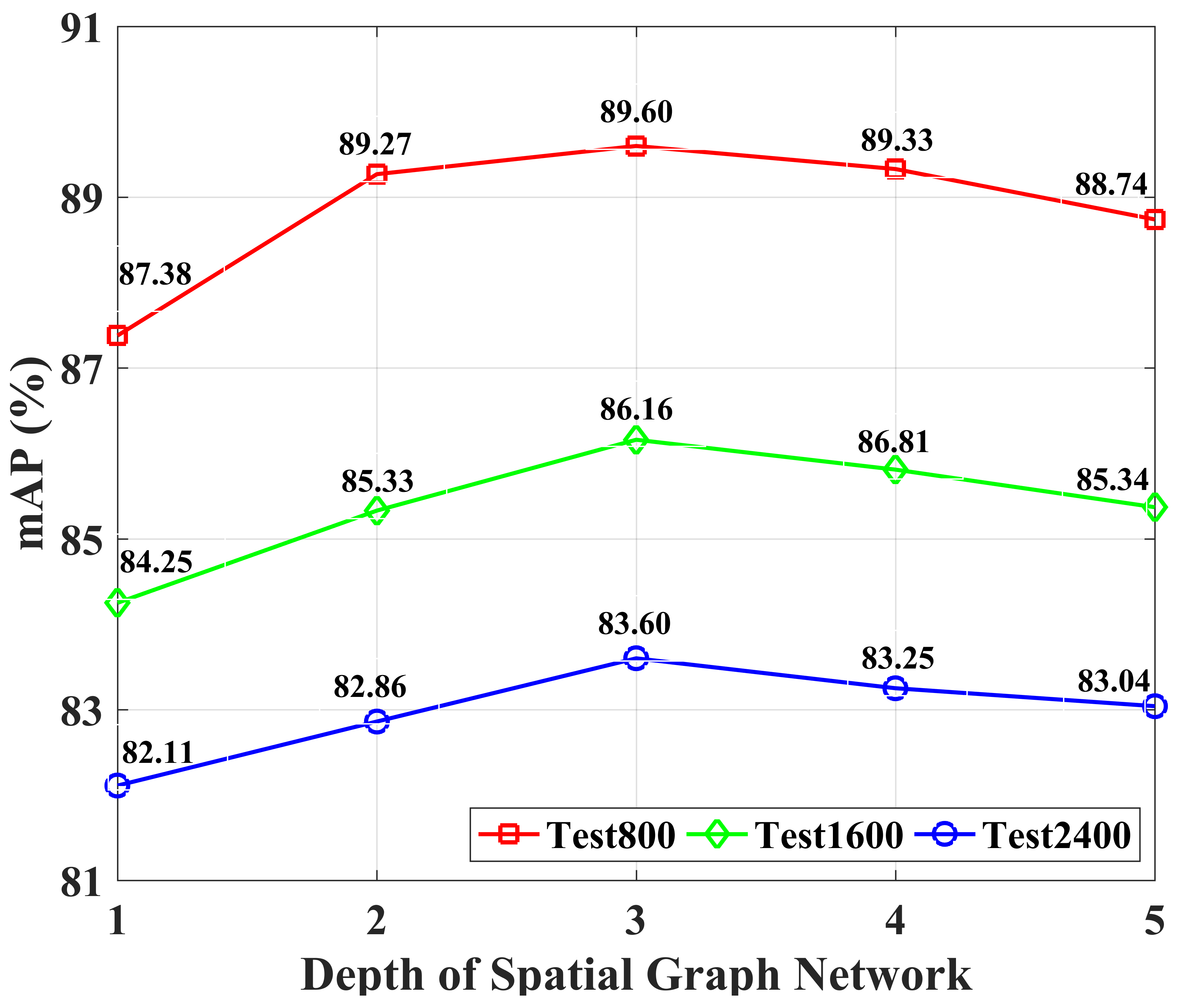
Figure 4: The mean average precision (mAP) comparison among spatial graph networks of different depths on VehicleID.

IV-D1 Role of PGN

To validate the role of PGN, HPGN is compared with a baseline method that replaces the PGN with a global max pooling (GMP) layer while holds the same backbone network to HPGN. As shown in Table V, HPGN significantly outperforms the baseline method. For example, compared to the baseline method, on VeRi776 [38], HPGN holds a larger 5.53% mAP, and on Test2400 of VehicleID [12], HPGN holds a larger 4.06% mAP. Those comparisons overall demonstrate the PGN can significantly improve vehicle re-identification.

Considering that PGN includes two essential designs, i.e., the spatial graph network (SGN) and the pyramidal architecture (PA), more ablations are investigated. Two different simplified HPGN, i.e., HPGN_OI and HPGN_NG, are constructed. HPGN_OI and HPGN_NG also use the same backbone network to HPGN. Besides, they hold a pyramidal architecture (PA) containing the same scale configuration to that of HPGN. However, the differences are as follows. (1) HPGN_OI Only retains a node Itself and gives up aggregating the node’s spatial neighbors (i.e., setting $S=\bm{0}$ in Eq. (3)) during the spatial graph network’s propagation. (2) HPGN_NG contains No spatial Graph network, that is, it entirely disregards spatial graph networks in its pyramidal architecture.

Comparing HPGN_OI, HPGN_NG, and HPGN, one can observe that HPGN_OI is better than HPGN_NG from Table V, demonstrating the beneficial effect of re-weighting nodes. Moreover, HPGN outperforms HPGN_OI, which suggests that aggregating both a node and the node’s neighbors can feed more information to improve the effect of re-weighting nodes. Besides, HPGN_NG is superior to the Baseline that replaces the PGN with a global max pooling (GMP) layer, which shows that the plain pyramidal architecture containing no SGN still is helpful to improve vehicle re-identification.

IV-D2 Influence of Changing SGN’s Depths

Fig. 3 shows the rank-1 identification rate (R1) comparison among SGNs of different depths (i.e., numbers of spatial graphs), and Fig. 4 presents the mAP comparison among those SGNs. It can be observed that both R1 and mAP performance fluctuate with SGN’s depths, and the best R1 and mAP are acquired when each SGN’s depth is set to 3. Furthermore, one can see even the worst results (i.e., those R1s and mAPs resulted from setting each SGN’s depth to 1) are comparable with the results of HPGN_NG (see Table V). These comparison results demonstrate the beneficial role of using SGNs again.

IV-D3 Impact of Varying HPGN’s Scale Configurations

In addition to the Baseline and HPGN showed in Table V, three HPGNs of different scale configured PGNs, namely, HPGN1, HPGN2, and HPGN3, are further evaluated. As shown in Table VI, HPGN1 represents that the applied PGN contains S5 and S4 scales. HPGN2 denotes that the used PGN includes S5, S4, and S3 scales. HPGN3 represents that the adopted PGN contains S5, S4, S3, and S2 scales. The HPGN applies a PGN that has S5, S4, S3, S2, and S1 scales. The Baseline only uses the S5 scale. The structures of S1, S2, S3, S4, and S5 can be found in Fig. 2. All these methods use the same backbone network.

From Table VI, it can be observed that the more scales applied in a PGN, the better performance will be acquired on both VeRi776 [38], VehicleID [12], and VeRi-Wild [39]. For example, on VeRi776 [38], HPGN’s mAP is 5.53%, 1.27%, 1.15%, and 0.83% higher than that of Baseline, HPGN1, HPGN2, and HPGN3, respectively. On the largest testing subset (i.e., Test2400) of VehicleID [12], HPGN defeats Baseline, HPGN1, HPGN2, and HPGN3 by 4.52%, 2.76%, 1.36%, and 1.27% higher rank-1 identification rates, respectively. These results demonstrate that the proposed HPGN exploring spatial significance of feature maps at multiple scales helps promote vehicle re-identification performance.

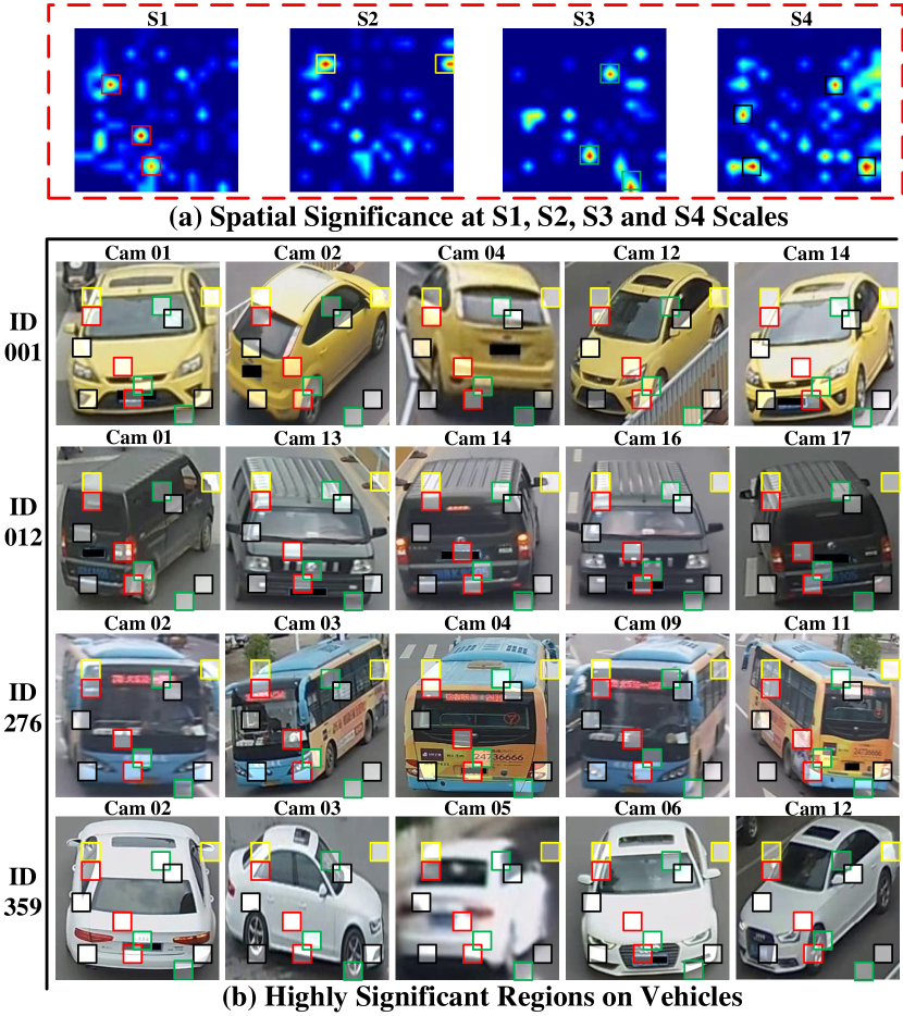
Figure 5: Visualization results on VeRi776.

IV-D4 Spatial Significance Visualization

The spatial significance visualization is realized by using the gradient weighted class activation mapping (Grad-CAM) [92] method to visualize the PGN’s learnable parameter matrixes (i.e., $\varTheta$ in Eq. (4)), as shown in Fig. 5 (a), where the higher significant regions are rendered in hotter colors (e.g., red), while the lower significant regions are rendered in cool colors (e.g., blue). The S1, S2, S3 and S4 scale configurations can be found in Fig. 2.

Two interesting observations can be found. First, at each scale, highly significant regions appear scatteredly, which demonstrates that the global pooling operation equally treats each region will lose the useful spatial significance information. Second, at four different scales, highly significant regions appear at different locations, which shows that there is a complementation of exploring spatial significance at multiple scales.

To further illustrate spatial significance, those highly significant regions explored in Fig. 5 (a) are served as observation windows on vehicle images captured from different cameras. As shown in Fig. 5 (b), informative parts (e.g., lightings, license plates, wheels, stickers or pendants on windshields) of vehicles are frequently observed, demonstrating the proposed HPGN method can explore spatial significance effectively.

V Conclusion

In this paper, a hybrid pyramidal graph network (HPGN) is proposed for vehicle re-identification. The HPGN consists of a backbone network (i.e., ResNet-50) and a novel pyramidal graph network (PGN). The backbone network is applied to extract feature maps from vehicle images, the PGN is designed to work behind the backbone network to comprehensively explore spatial significance of the feature maps at multiple scales. The key module of PGN is the innovative spatial graph network (SGN), which stacks a list of spatial graphs (SGs) on feature maps of a specific scale and explore the spatial significance via re-weighting nodes during the propagation. Experiments on three large scale databases demonstrate that the proposed HPGN method outperforms state-of-the-art vehicle re-identification approaches.

References

- [1] X. Liu, W. Liu, H. Ma, and H. Fu, “Large-scale vehicle re-identification in urban surveillance videos,” in International Conference on Multimedia & Expo, 2016, pp. 1–6.
- [2] X. Liu, W. Liu, T. Mei, and H. Ma, “Provid: Progressive and multi-modal vehicle re-identification for large-scale urban surveillance,” IEEE Transactions on Multimedia, vol. 20, no. 3, pp. 645–658, 2018.
- [3] K. Simonyan and A. Zisserman, “Very deep convolutional networks for large-scale image recognition,” in International Conference on Learning Representations, 2015.
- [4] C. Szegedy, W. Liu, Y. Jia, P. Sermanet, S. Reed, D. Anguelov, D. Erhan, V. Vanhoucke, and A. Rabinovich, “Going deeper with convolutions,” in Conference on Computer Vision and Pattern Recognition, 2015, pp. 1–9.
- [5] K. He, X. Zhang, S. Ren, and J. Sun, “Deep residual learning for image recognition,” in Conference on Computer Vision and Pattern Recognition, 2016, pp. 770–778.
- [6] K. He, X. Zhang, S. Ren, and J. Sun, “Identity mappings in deep residual networks,” in European Conference on Computer Vision, 2016, pp. 630–645.
- [7] G. Huang, Z. Liu, L. van der Maaten, and K. Q. Weinberger, “Densely connected convolutional networks,” in Conference on Computer Vision and Pattern Recognition, 2017, pp. 2261–2269.
- [8] A. G. Howard, M. Zhu, B. Chen, D. Kalenichenko, W. Wang, T. Weyand, M. Andreetto, and H. Adam, “Mobilenets: Efficient convolutional neural networks for mobile vision applications,” 2017.
- [9] K. Yan, Y. Tian, Y. Wang, W. Zeng, and T. Huang, “Exploiting multi-grain ranking constraints for precisely searching visually-similar vehicles,” in International Conference on Computer Vision, 2017, pp. 562–570.
- [10] P. Khorramshahi, A. Kumar, N. Peri, S. S. Rambhatla, J.-C. Chen, and R. Chellappa, “A dual-path model with adaptive attention for vehicle re-identification,” in International Conference on Computer Vision, 2019, pp. 6132–6141.
- [11] Y. Zhang, D. Liu, and Z.-J. Zha, “Improving triplet-wise training of convolutional neural network for vehicle re-identification,” in International Conference on Multimedia & Expo, 2017, pp. 1386–1391.
- [12] H. Liu, Y. Tian, Y. Wang, L. Pang, and T. Huang, “Deep relative distance learning: Tell the difference between similar vehicles,” in Conference on Computer Vision and Pattern Recognition, 2016, pp. 2167–2175.
- [13] Y. Li, Y. Li, H. Yan, and J. Liu, “Deep joint discriminative learning for vehicle re-identification and retrieval,” in International Conference on Image Processing, 2017, pp. 395–399.
- [14] N. Jiang, Y. Xu, Z. Zhou, and W. Wu, “Multi-attribute driven vehicle re-identification with spatial-temporal re-ranking,” in International Conference on Image Processing, 2018, pp. 858–862.
- [15] R. Chu, Y. Sun, Y. Li, Z. Liu, C. Zhang, and Y. Wei, “Vehicle re-identification with viewpoint-aware metric learning,” in International Conference on Computer Vision, 2019, pp. 8282–8291.
- [16] Y. Shen, T. Xiao, H. Li, S. Yi, and X. Wang, “Learning deep neural networks for vehicle re-id with visual-spatio-temporal path proposals,” in International Conference on Computer Vision, 2017, pp. 1918–1927.
- [17] H. Guo, C. Zhao, Z. Liu, J. Wang, and H. Lu, “Learning coarse-to-fine structured feature embedding for vehicle re-identification,” in AAAI Conference on Artificial Intelligence, 2018, pp. 6853–6860.
- [18] R. Kumar, E. Weill, F. Aghdasi, and P. Sriram, “Vehicle re-identification: an efficient baseline using triplet embedding,” in International Joint Conference on Neural Networks, 2019, pp. 1–9.
- [19] A. Kanacı, X. Zhu, and S. Gong, “Vehicle re-identification in context,” in German Conference on Pattern Recognition, 2018, pp. 377–390.
- [20] Y. Xu, N. Jiang, L. Zhang, Z. Zhou, and W. Wu, “Multi-scale vehicle re-identification using self-adapting label smoothing regularization,” in IEEE International Conference on Acoustics, Speech and Signal Processing, 2019, pp. 2117–2121.
- [21] Y. Lou, Y. Bai, J. Liu, S. Wang, and L.-Y. Duan, “Embedding adversarial learning for vehicle re-identification,” IEEE Transactions on Image Processing, pp. 3794–3807, 2019.
- [22] J. Peng, H. Wang, F. Xu, and X. Fu, “Cross domain knowledge learning with dual-branch adversarial network for vehicle re-identification,” Neurocomputing, 2020.
- [23] H. Chen, B. Lagadec, and F. Bremond, “Partition and reunion: A two-branch neural network for vehicle re-identification,” in Conference on Computer Vision and Pattern Recognition Workshops, 2019, pp. 184–192.
- [24] J. Zhu, H. Zeng, J. Huang, S. Liao, L. Zhen, C. Cai, and L. Zheng, “Vehicle re-identification using quadruple directional deep learning features,” Transactions on Intelligent Transportation Systems, vol. 21, no. 1, pp. 410–420, 2020.
- [25] J. Zhu, J. Huang, H. Zeng, X. Ye, B. Li, Z. Lei, and L. Zheng, “Object reidentification via joint quadruple decorrelation directional deep networks in smart transportation,” IEEE Internet of Things Journal, vol. 7, no. 4, pp. 2944–2954, 2020.
- [26] X. Liu, S. Zhang, Q. Huang, and W. Gao, “Ram: a region-aware deep model for vehicle re-identification,” in International Conference on Multimedia & Expo, 2018, pp. 1–6.
- [27] J. Qian, W. Jiang, H. Luo, and H. Yu, “Stripe-based and attribute-aware network: A two-branch deep model for vehicle re-identification,” Measurement Science and Technology, 2020.
- [28] C. Liu, D. Q. Huynh, and M. Reynolds, “Urban area vehicle re-identification with self-attention stair feature fusion and temporal bayesian re-ranking,” in International Joint Conference on Neural Networks, 2019, pp. 1–8.
- [29] X. Ma, K. Zhu, H. Guo, J. Wang, M. Huang, and Q. Miao, “Vehicle re-identification with refined part model,” in International Conference on Multimedia & Expo Workshops, 2019, pp. 603–606.
- [30] H. Guo, K. Zhu, M. Tang, and J. Wang, “Two-level attention network with multi-grain ranking loss for vehicle re-identification,” IEEE Transactions on Image Processing, pp. 4328–4338, 2019.
- [31] M. Jaderberg, K. Simonyan, A. Zisserman et al., “Spatial transformer networks,” in Advances in Neural Information Processing Systems, 2015, pp. 2017–2025.
- [32] B. He, J. Li, Y. Zhao, and Y. Tian, “Part-regularized near-duplicate vehicle re-identification,” in Conference on Computer Vision and Pattern Recognition, 2019, pp. 3997–4005.
- [33] X. Zhang, R. Zhang, J. Cao, D. Gong, M. You, and C. Shen, “Part-guided attention learning for vehicle re-identification,” arXiv preprint arXiv:1909.06023, 2019.
- [34] Y. Sun, M. Li, and J. Lu, “Part-based multi-stream model for vehicle searching,” in International Conference on Pattern Recognition, 2018, pp. 1372–1377.
- [35] Z. Wang, L. Tang, X. Liu, Z. Yao, S. Yi, J. Shao, J. Yan, S. Wang, H. Li, and X. Wang, “Orientation invariant feature embedding and spatial temporal regularization for vehicle re-identification,” in International Conference on Computer Vision, 2017, pp. 379–387.
- [36] P. Khorramshahi, N. Peri, A. Kumar, A. Shah, and R. Chellappa, “Attention driven vehicle re-identification and unsupervised anomaly detection for traffic understanding,” in Computer Vision and Pattern Recognition Workshops, 2019, pp. 239–246.
- [37] Z. Tang, M. Naphade, S. Birchfield, J. Tremblay, W. Hodge, R. Kumar, S. Wang, and X. Yang, “Pamtri: Pose-aware multi-task learning for vehicle re-identification using highly randomized synthetic data,” in International Conference on Computer Vision, 2019, pp. 211–220.
- [38] X. Liu, W. Liu, T. Mei, and H. Ma, “A deep learning-based approach to progressive vehicle re-identification for urban surveillance,” in European Conference on Computer Vision, 2016, pp. 869–884.
- [39] Y. Lou, Y. Bai, J. Liu, S. Wang, and L. Duan, “Veri-wild: A large dataset and a new method for vehicle re-identification in the wild,” in Conference on Computer Vision and Pattern Recognition, 2019, pp. 3235–3243.
- [40] H. Zhang, I. Goodfellow, D. Metaxas, and A. Odena, “Self-attention generative adversarial networks,” stat, vol. 1050, p. 21, 2018.
- [41] F. Wang, M. Jiang, C. Qian, S. Yang, C. Li, H. Zhang, X. Wang, and X. Tang, “Residual attention network for image classification,” in Conference on Computer Vision and Pattern Recognition, 2017, pp. 3156–3164.
- [42] S. Ren, K. He, R. Girshick, and J. Sun, “Faster r-cnn: Towards real-time object detection with region proposal networks,” in Annual Conference on Neural Information Processing Systems, 2015, pp. 91–99.
- [43] J. Redmon, S. Divvala, R. Girshick, and A. Farhadi, “You only look once: Unified, real-time object detection,” in Conference on Computer Vision and Pattern Recognition, 2016, pp. 779–788.
- [44] W. Liu, D. Anguelov, D. Erhan, C. Szegedy, S. Reed, C.-Y. Fu, and A. C. Berg, “Ssd: Single shot multibox detector,” in European Conference on Computer Vision, 2016, pp. 21–37.
- [45] S. Ioffe and C. Szegedy, “Batch normalization: Accelerating deep network training by reducing internal covariate shift,” in International Conference on Machine Learning, 2015, pp. 448–456.
- [46] V. Nair and G. E. Hinton, “Rectified linear units improve restricted boltzmann machines,” in International Conference on Machine Learning, 2010, pp. 807–814.
- [47] Z. Zheng, L. Zheng, and Y. Yang, “Unlabeled samples generated by gan improve the person re-identification baseline in vitro,” in International Conference on Computer Vision, 2017, pp. 3754–3762.
- [48] Y. Sun, X. Wang, and X. Tang, “Deep learning face representation from predicting 10,000 classes,” in Conference on Computer Vision and Pattern Recognition, 2014, pp. 1891–1898.
- [49] F. Schroff, D. Kalenichenko, and J. Philbin, “Facenet: A unified embedding for face recognition and clustering,” in Conference on Computer Vision and Pattern Recognition, 2015, pp. 815–823.
- [50] X. Liu, S. Zhang, X. Wang, R. Hong, and Q. Tian, “Group-group loss-based global-regional feature learning for vehicle re-identification,” IEEE Transactions on Image Processing, vol. 29, pp. 2638–2652, 2019.
- [51] Y. Bai, Y. Lou, F. Gao, S. Wang, Y. Wu, and L.-Y. Duan, “Group-sensitive triplet embedding for vehicle reidentification,” IEEE Transactions on Multimedia, vol. 20, no. 9, pp. 2385–2399, 2018.
- [52] W. Lin, Y. Li, X. Yang, P. Peng, and J. Xing, “Multi-view learning for vehicle re-identification,” in International Conference on Multimedia & Expo, 2019, pp. 832–837.
- [53] T. Kipf and M. Welling, “Semi-supervised classification with graph convolutional networks,” in International Conference on Learning Representations, 2017.
- [54] Z. Ying, J. You, C. Morris, X. Ren, W. Hamilton, and J. Leskovec, “Hierarchical graph representation learning with differentiable pooling,” in Advances in neural information processing systems, 2018, pp. 4800–4810.
- [55] M. Zhang, Z. Cui, M. Neumann, and Y. Chen, “An end-to-end deep learning architecture for graph classification,” in AAAI Conference on Artificial Intelligence, 2018.
- [56] Z.-M. Chen, X.-S. Wei, P. Wang, and Y. Guo, “Multi-label image recognition with graph convolutional networks,” in Conference on Computer Vision and Pattern Recognition, 2019, pp. 5177–5186.
- [57] R. Vemulapalli, F. Arrate, and R. Chellappa, “Human action recognition by representing 3d skeletons as points in a lie group,” in Conference on Computer Vision and Pattern Recognition, 2014, pp. 588–595.
- [58] L. Shi, Y. Zhang, J. Cheng, and H. Lu, “Two-stream adaptive graph convolutional networks for skeleton-based action recognition,” in Conference on Computer Vision and Pattern Recognition, 2019, pp. 12 026–12 035.
- [59] M. Li, S. Chen, X. Chen, Y. Zhang, Y. Wang, and Q. Tian, “Actional-structural graph convolutional networks for skeleton-based action recognition,” in Conference on Computer Vision and Pattern Recognition, 2019, pp. 3595–3603.
- [60] Y. Shen, H. Li, S. Yi, D. Chen, and X. Wang, “Person re-identification with deep similarity-guided graph neural network,” in European Conference on Computer Vision, 2018, pp. 486–504.
- [61] Z. Huang, Z. Wang, W. Hu, C.-W. Lin, and S. Satoh, “Dot-gnn: Domain-transferred graph neural network for group re-identification,” in ACM International Conference on Multimedia, 2019, pp. 1888–1896.
- [62] L. Bao, B. Ma, H. Chang, and X. Chen, “Masked graph attention network for person re-identification,” in Conference on Computer Vision and Pattern Recognition Workshops, 2019, pp. 0–0.
- [63] M. Ye, A. J. Ma, L. Zheng, J. Li, and P. C. Yuen, “Dynamic label graph matching for unsupervised video re-identification,” in International Conference on Computer Vision, 2017, pp. 5142–5150.
- [64] D. Cheng, Y. Gong, X. Chang, W. Shi, A. Hauptmann, and N. Zheng, “Deep feature learning via structured graph laplacian embedding for person re-identification,” Pattern Recognition, vol. 82, pp. 94–104, 2018.
- [65] H. Luo, W. Jiang, Y. Gu, F. Liu, X. Liao, S. Lai, and J. Gu, “A strong baseline and batch normalization neck for deep person re-identification,” IEEE Transactions on Multimedia (Early Access), 2019.
- [66] X. Yang, C. Lang, P. Peng, and J. Xing, “Vehicle re-identification by multi-grain learning,” in International Conference on Image Processing, 2019, pp. 3113–3117.
- [67] M. Wu, Y. Zhang, T. Zhang, and W. Zhang, “Background segmentation for vehicle re-identification,” in Springer International Conference on Multimedia Modeling, 2020, pp. 88–99.
- [68] B. Xu, N. Wang, T. Chen, and M. Li, “Empirical evaluation of rectified activations in convolutional network,” arXiv preprint arXiv:1505.00853, 2015.
- [69] A. Hermans, L. Beyer, and B. Leibe, “In defense of the triplet loss for person re-identification,” arXiv preprint arXiv:1703.07737, 2017.
- [70] A. Paszke, S. Gross, F. Massa, A. Lerer, J. Bradbury, G. Chanan, T. Killeen, Z. Lin, N. Gimelshein, L. Antiga, A. Desmaison, A. Kopf, E. Yang, Z. DeVito, M. Raison, A. Tejani, S. Chilamkurthy, B. Steiner, L. Fang, J. Bai, and S. Chintala, “Pytorch: An imperative style, high-performance deep learning library,” in Advances in Neural Information Processing Systems, 2019, pp. 8024–8035.
- [71] Z. Zhong, L. Zheng, G. Kang, S. Li, and Y. Yang, “Random erasing data augmentation,” in AAAI Conference on Artificial Intelligence, 2020.
- [72] A. Krizhevsky, I. Sutskever, and G. E. Hinton, “Imagenet classification with deep convolutional neural networks,” in Annual Conference on Neural Information Processing Systems, 2012, pp. 1097–1105.
- [73] Y. He, C. Dong, and Y. Wei, “Combination of appearance and license plate features for vehicle re-identification,” in International Conference on Image Processing, 2019, pp. 3108–3112.
- [74] A. Shankar, A. Poojary, C. Y. Varghese Kollerathu, S. Reddy, and V. Sudhakaran, “Comparative study of various losses for vehicle re-identification,” in Conference on Computer Vision and Pattern Recognition Workshops, 2019, pp. 256–264.
- [75] A. Kanaci, M. Li, S. Gong, and G. Rajamanoharan, “Multi-task mutual learning for vehicle re-identification,” in Computer Vision and Pattern Recognition Workshops, 2019, pp. 62–70.
- [76] J. Peng, H. Wang, T. Zhao, and X. Fu, “Learning multi-region features for vehicle re-identification with context-based ranking method,” Neurocomputing, vol. 359, pp. 427–437, 2019.
- [77] G. Chen, T. Zhang, J. Lu, and J. Zhou, “Deep meta metric learning,” in International Conference on Computer Vision, 2019, pp. 9547–9556.
- [78] Z. Tang, M. Naphade, M.-Y. Liu, X. Yang, S. Birchfield, S. Wang, R. Kumar, D. Anastasiu, and J.-N. Hwang, “Cityflow: A city-scale benchmark for multi-target multi-camera vehicle tracking and re-identification,” in Conference on Computer Vision and Pattern Recognition, 2019, pp. 8797–8806.
- [79] S. Kan, Y. Cen, Z. He, Z. Zhang, L. Zhang, and Y. Wang, “Supervised deep feature embedding with hand crafted feature,” IEEE Transactions on Image Processing, vol. 28, no. 12, pp. 5809–5823, 2019.
- [80] S. A. S. Alfasly, Y. Hu, T. Liang, X. Jin, Q. Zhao, and B. Liu, “Variational representation learning for vehicle re-identification,” in International Conference on Image Processing, 2019, pp. 3118–3122.
- [81] C.-T. Liu, M.-Y. Lee, C.-W. Wu, B.-Y. Chen, T.-S. Chen, Y.-T. Hsu, S.-Y. Chien, and N. I. Center, “Supervised joint domain learning for vehicle re-identification,” in Computer Vision and Pattern Recognition Workshops, 2019, pp. 45–52.
- [82] Y. Zhou, L. Shao, and A. Dhabi, “Viewpoint-aware attentive multi-view inference for vehicle re-identification,” in Conference on Computer Vision and Pattern Recognition, 2018, pp. 6489–6498.
- [83] J. Zhu, H. Zeng, Z. Lei, L. Zheng, and C. Cai, “A shortly and densely connected convolutional neural network for vehicle re-identification,” in International Conference on Pattern Recognition, 2018, pp. 3285–3290.
- [84] Y. Zhou, L. Liu, and L. Shao, “Vehicle re-identification by deep hidden multi-view inference,” IEEE Transactions on Image Processing, vol. 27, no. 7, pp. 3275–3287, 2018.
- [85] Y. Zhou and L. Shao, “Vehicle re-identification by adversarial bi-directional lstm network,” in Winter Conference on Applications of Computer Vision, 2018, pp. 653–662.
- [86] L. Yang, P. Luo, C. L. Chen, and X. Tang, “A large-scale car dataset for fine-grained categorization and verification,” in Conference on Computer Vision and Pattern Recognition, 2015, pp. 3973–3981.
- [87] Y. Zhao, C. Shen, H. Wang, and S. Chen, “Structural analysis of attributes for vehicle re-identification and retrieval,” IEEE Transactions on Intelligent Transportation Systems (Early Access), 2019.
- [88] J. Hou, H. Zeng, J. Zhu, J. Hou, J. Chen, and K.-K. Ma, “Deep quadruplet appearance learning for vehicle re-identification,” IEEE Transactions on Vehicular Technology, vol. 68, no. 9, pp. 8512–8522, 2019.
- [89] J. Hou, H. Zeng, L. Cai, J. Zhu, J. Chen, and K.-K. Ma, “Multi-label learning with multi-label smoothing regularization for vehicle re-identification,” Neurocomputing, vol. 345, pp. 15–22, 2019.
- [90] J.-Y. Zhu, T. Park, P. Isola, and A. A. Efros, “Unpaired image-to-image translation using cycle-consistent adversarial networks,” in International Conference on Computer Vision, 2017, pp. 2223–2232.
- [91] Y. Yuan, K. Yang, and C. Zhang, “Hard-aware deeply cascaded embedding,” in International Conference on Computer Vision, 2017, pp. 814–823.
- [92] R. R. Selvaraju, M. Cogswell, A. Das, R. Vedantam, D. Parikh, and D. Batra, “Grad-cam: Visual explanations from deep networks via gradient-based localization,” in International Conference on Computer Vision, 2017, pp. 618–626.