The $Gaia$-$Kepler$ Stellar Properties Catalog. II. Planet Radius Demographics as a Function of Stellar Mass and Age

Abstract

Studies of exoplanet demographics require large samples and precise constraints on exoplanet host stars. Using the homogeneous $Kepler$ stellar properties derived using $Gaia$ Data Release 2 by Berger et al. (2020), we re-compute $Kepler$ planet radii and incident fluxes and investigate their distributions with stellar mass and age. We measure the stellar mass dependence of the planet radius valley to be $d\log R_{\mathrm{p}}$/$d\log M_{\star}$ = $0.26^{+0.21}_{-0.16}$, consistent with the slope predicted by a planet mass dependence on stellar mass (0.24–0.35) and core-powered mass-loss (0.33). We also find first evidence of a stellar age dependence of the planet populations straddling the radius valley. Specifically, we determine that the fraction of super-Earths (1–1.8 $\mathrm{R_{\oplus}}$) to sub-Neptunes (1.8–3.5 $\mathrm{R_{\oplus}}$) increases from 0.61 $\pm$ 0.09 at young ages ($<$ 1 Gyr) to 1.00 $\pm$ 0.10 at old ages ($>$ 1 Gyr), consistent with the prediction by core-powered mass-loss that the mechanism shaping the radius valley operates over Gyr timescales. . We confirm the existence of planets within the hot sub-Neptunian “desert” (2.2 $<$ $R_{\mathrm{p}}$ $<$ 3.8 $\mathrm{R_{\oplus}}$, $F_{\mathrm{p}}$ $>$ 650 $\mathrm{F_{\oplus}}$) and show that these planets are preferentially orbiting more evolved stars compared to other planets at similar incident fluxes. In addition, we identify candidates for cool ($F_{\mathrm{p}}$ $<$ 20 $\mathrm{F_{\oplus}}$) inflated Jupiters, present a revised list of habitable zone candidates, and find that the ages of single- and multiple-transiting planet systems are statistically indistinguishable.

1 Introduction

One of the most impactful exoplanet discoveries in recent years has been the planet radius “valley”, a dip in the occurrence of Kepler planets at $\approx$ 1.9 $\mathrm{R_{\oplus}}$ separating super-Earth and sub-Neptune-sized exoplanets (Owen & Wu, 2013; Fulton et al., 2017; Fulton & Petigura, 2018). The discovery of the radius valley was enabled by precise stellar parameters for subsamples of Kepler host stars, such as those derived in the California-Kepler Survey (CKS, Petigura et al., 2017; Johnson et al., 2017) and from asteroseismic constraints (Van Eylen et al., 2018). More recently, Gaia parallaxes (Gaia Collaboration et al., 2018; Lindegren et al., 2018) have better constrained the stellar radii of the vast majority of Kepler host stars, followed by more detailed investigations of the valley as a function of stellar mass (Fulton & Petigura, 2018), metallicity (Owen & Murray-Clay, 2018), planet orbital period, and stellar incident flux (Berger et al., 2018b; Fulton & Petigura, 2018). Most recently, the radius valley has also been identified in the $K2$ sample (Hardegree-Ullman et al., 2020; Cloutier & Menou, 2020).

Several models have been proposed to explain the planet radius valley, including planet formation in a gas-poor disk (Lee et al., 2014; Lee & Chiang, 2016), extreme ultraviolet (EUV) photoevaporation of planet atmospheres (Owen & Wu, 2013, 2017; Owen & Murray-Clay, 2018; Lopez & Rice, 2018; Wu, 2019), and core-powered mass-loss (Ginzburg et al., 2016, 2018; Gupta & Schlichting, 2019, 2020). Currently, photoevaporation and core-powered mass-loss are the two leading theories that can effectively explain the dependence of the gap on stellar mass, orbital period, and incident flux. However, observational studies have not yet been able to differentiate between these two theories. For example, to explain the radius valley as a function of stellar mass, photoevaporation requires a planet mass dependence on stellar mass (Wu, 2019). Multi-transiting systems hosting planets with mass measurements and radii both above and below the gap can distinguish between these models, but only a few examples are available (e.g., Cloutier et al., 2020; Nowak et al., 2020).

Stellar ages provide a new dimension to determine the physical mechanisms shaping exoplanet populations. Exoplanet properties are expected to change over time, such as a decrease in their radii from cooling and contraction (Lopez et al., 2012) and atmosphere loss (Ginzburg et al., 2016; Owen & Wu, 2017) or an increase in orbital eccentricity due to dynamical interactions between planets (Weiss et al., 2018). However, ages are difficult to determine for stellar populations, such as Kepler host stars, because available methods differ considerably across the Hertzprung-Russell (H-R) diagram. For instance, isochrone ages are effective on the upper main sequence ($M_{\star}$ $\gtrsim$ 1 $\mathrm{M_{\odot}}$), but are uninformative on the lower main sequence, where stellar rotation, activity, and lithium abundances provide more discriminatory power (Pont & Eyer, 2004; Epstein & Pinsonneault, 2014). Asteroseismology provides precise stellar ages, but is generally only available for a small subset of mostly evolved exoplanet host stars (Silva Aguirre et al., 2015).

So far, only a few studies have compared properties of exoplanets orbiting stars of different ages. Berger et al. (2018a) found tentative evidence for the shrinking of planetary radii with stellar age based on the lithium abundances of CKS planet hosts differentiated by the Hyades 650 Myr empirical lithium abundance (A(Li))–$T_{\mathrm{eff}}$ curve (Boesgaard et al., 2016). Additionally, the Zodiacal Exoplanets In Time (ZEIT) survey yielded evidence for larger, younger planets in clusters where ages are already known (Mann et al., 2018). While both core-powered mass-loss and photoevaporation predict that the ratio of super-Earths to sub-Neptunes should increase over time, their timescales are very different: photoevaporation acts on timescales of $\sim$ 100 Myr (Lopez et al., 2012; Owen & Wu, 2017) and core-powered mass-loss acts on timescales of $\sim$ Gyr (Gupta & Schlichting, 2019, 2020). Stellar ages are also critical to address other open questions in exoplanet radius demographics, such as the hot sub-Neptunian desert (Lundkvist et al., 2016; Berger et al., 2018b; Dong et al., 2018), hot Jupiter inflation (Guillot & Showman, 2002; Fortney & Nettelmann, 2010; Baraffe et al., 2010, 2014; Laughlin & Lissauer, 2015; Laughlin, 2018; Komacek et al., 2020), and the dynamical evolution of multiplanet systems (Armitage & Rice, 2005; Spalding & Batygin, 2016; Rizzuto, 2017; Weiss et al., 2018).

Previous Kepler stellar properties catalogs have not estimated ages due to inhomogeneous input parameters and the lack of precise parallaxes (Huber et al., 2014; Mathur et al., 2017). Here, we re-derive and analyze planet parameters using the updated stellar parameters by Berger et al. (2020) (1 hereafter), the first homogeneous catalog of stellar $T_{\mathrm{eff}}$, $\log g$, radii, masses, densities, luminosities, and ages of Kepler stars.

2 Sample Selection and Methodology

2.1 Host Star and Planet Sample

First, we downloaded the KOI table on 10/13/19 from the NASA Exoplanet Archive, including 9564 planet candidates. Then, we cross-matched this table with our Table 2 in 1, leaving 8875 planets. To avoid using stars with likely binary companions, we eliminated all stars with Gaia DR2 re-normalized unit-weight error (RUWE) $>$ 1.2 (Evans, 2018; Rizzuto et al., 2018; Bryson et al., 2020, 1, and see Kraus et al. in prep). In addition, we discarded stars with unreliable isochrone-derived parameters (iso_gof $<$ 0.99, 1). We also removed all planets designated as false positives according to the koi_disposition flag and those without reported planet-to-star radius ratios. We did not remove adaptive optics (AO)-detected binaries (Furlan et al., 2017) to preserve number statistics, but we comment on their influence where relevant. Following these sample cuts, we retained 2956 stars hosting 3898 planets.

2.2 Updated Planet Parameters

We computed the updated planet radii utilizing the planet-to-star radius ratios provided in the KOI table from the NASA Exoplanet Archive and the stellar radii computed in 1. In addition, we updated semimajor axes using the stellar masses in 1 and the orbital periods in Thompson et al. (2018). Finally, we updated the incident fluxes for each planet by using the semimajor axes and the stellar luminosities from 1. We tested the effect of our new stellar parameters on the planet-to-star radius ratios by computing new planet-to-star radius ratios using the transit period, duration, and depth values from Thompson et al. (2018), the quadratic limb darkening coefficients from Claret & Bloemen (2011), Equation (9) from Seager & Mallén-Ornelas (2003), and the small-planet-limit version of Equation (8) from Mandel & Agol (2002). We found that the differences between the Mathur et al. (2017)-derived and 1-derived planet-to-star radius ratios were on the order of 3% and within the 8% median uncertainty in Thompson et al. (2018). Therefore, these systematic effects are small and we neglect them here. We provide all of our planet parameters in Table 1.

3 Kepler Planet Host Stars

Figure 1: Histograms of host star properties. The black dashed vertical lines illustrate the median value for each parameter. In Panel (b) we plot both the overall host sample (black) and those with reliable ages (red).

3.1 Histograms

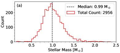
We plot histograms of physical parameters of the host star sample in Figure 1. Figure 1(a) shows the distribution of masses, which peak at solar mass, with a lower 1$\sigma$ bound of 0.78 $\mathrm{M_{\odot}}$ and an upper 1$\sigma$ bound of 1.19 $\mathrm{M_{\odot}}$. The lowest and highest mass hosts are 0.14 $\mathrm{M_{\odot}}$ and 2.8 $\mathrm{M_{\odot}}$, respectively.

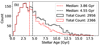
Figure 1(b) displays the distributions of stellar ages, separated into the entire host sample (black) and an “informative” age sample (red). The informative age distribution ignores any hosts that have terminal age of the main sequence (TAMS) $>$ 20 Gyr, which are stars that evolve too slowly in their main sequence lifetimes for isochrone-fitting to constrain their ages (1). The median ages are close to the age of the Sun, as expected from the Kepler target selection (Batalha et al., 2010). Both distributions peak at 3 Gyr with a tail towards old ages. Ages older than 14 Gyr occur because the 1 model grid of MESA (Paxton et al., 2011, 2013, 2015) Isochrones and Stellar Tracks (MIST v1.2 with rotation, Choi et al., 2016; Dotter, 2016) purposefully used an upper limit of 20 Gyr to minimize grid edge-effects, which can bias the parameter posteriors. The two distributions in Figure 1(b) differ the most at $\approx$ 10 Gyr, corresponding to M-dwarfs with uninformative ages producing flat posteriors with medians at half the age of the grid. The small number of hosts older than 14 Gyr are stars whose input parameters place them on or close to the edge of the grid. Some of these old hosts are probably cool main sequence binaries similar to those identified in Berger et al. (2018b), as stellar models are unable to reproduce their cool $T_{\mathrm{eff}}$ and large radii at the age of the universe. Finally, we note that the overall age distribution is consistent with asteroseismic ages provided by the APOKASC2 catalog of Kepler red giants (Pinsonneault et al., 2018).

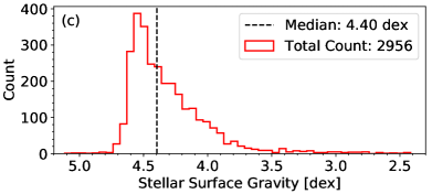
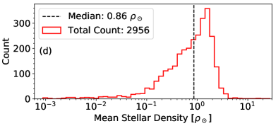
Figures 1(c) and 1(d) shows the stellar surface gravity ($\log g$) and mean stellar density distributions of Kepler host stars. These distributions are significantly different from the entire Kepler stellar sample, which has another, smaller peak at $\log g$ $\approx$ 2.5 dex and $\rho_{\star}$ $\approx$ $10^{-3}$ $\rho_{\odot}$. These peaks do not appear here because the percentage of giants with detected planets is much lower, given observational biases. Our median $\log g$ and $\rho_{\star}$ are slightly smaller than solar, and the tails to smaller values are comprised of subgiants (Verner et al., 2011; Everett et al., 2013; Gaidos & Mann, 2013; Huber et al., 2014). There are a few giant hosts at the lowest $\log g$ and density values, but many of these stars host unconfirmed, potential false positive planets (Sliski & Kipping, 2014).

3.2 The Host Star H-R Diagram

Figure 2: Hertzprung-Russell diagram of Kepler planet host stars, colored by their isochrone age (top, colors capped at 12 Gyr) and maximum absolute age uncertainties (bottom, colors capped at 6 Gyr). The grey points have uninformative ages (TAMS $>$ 20 Gyr) and/or low goodness-of-fit values. Nine stars hotter than 8000 K are omitted from this plot.

Figure 3: Planet radius versus incident flux for Kepler exoplanets. Points are colored according to the host star mass as indicated by the color bar on the right. Planet candidates are shown as translucent points. The dashed line box shows the sub-Neptunian desert identified in Lundkvist et al. (2016), and the green bar indicates the approximate “optimistic” habitable zone defined by Kane et al. (2016).

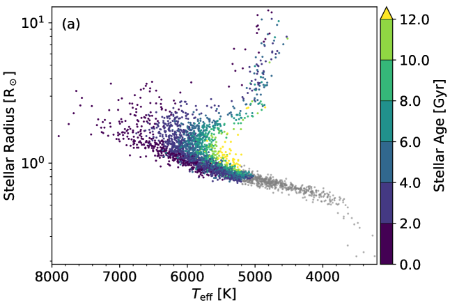
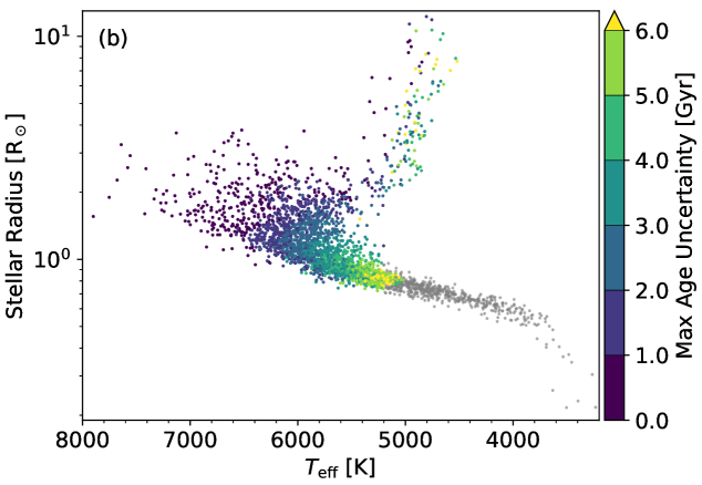
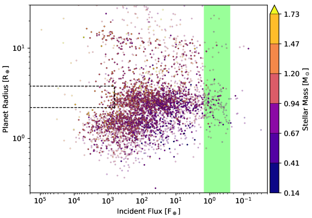
Figure 2 shows stellar radii versus temperature for the Kepler host star sample, color-coded by age and maximum absolute age uncertainty. For the hottest stars the age values and uncertainties are less than 2 Gyr. Both ages and age uncertainties increase smoothly towards cooler effective temperatures. Subgiants, compared to their main sequence counterparts, have smaller error bars due to rapid evolution on the subgiant branch, while their ages can vary significantly based on their $T_{\mathrm{eff}}$. On the giant branch, we also see that stars with the youngest ages and smallest age uncertainties are also the hottest and most massive, as more massive stars evolve more quickly than their lower mass counterparts. We note that giant ages are potentially unreliable because of the limitations of isochrone fitting with photometric colors and a solar neighborhood metallicity prior for stars that do not have spectroscopic measurements (see 1 for details).

The ages reach a maximum of $>$ 12 Gyr at the main sequence turnoff for the least massive stars, while the maximum age uncertainties increase towards the lower main sequence, until they reach $>$ 6 Gyr. Zero age main sequence (ZAMS) F stars have low age uncertainties between 0 and 2 Gyr, while ZAMS G-dwarfs have moderate age uncertainties between 1 and 5 Gyr. For K-dwarfs, the ZAMS uncertainties are typically larger than 6 Gyr. Some cool dwarfs with large/small radii have underestimated uncertainties due to grid edge effects. Finally, we see that all the late K–M-dwarfs have uninformative ages (TAMS $>$ 20 Gyr, 1). In particular, their observables provide limited information with which we can distinguish between the ages of these stars, which evolve slowly in the H-R diagram over 14 Gyr.

Figure 2 illustrates variation in the effectiveness of isochrone placement for different types of stars, from subgiants (very effective) to K- and M-dwarfs (not effective at all). In addition, it demonstrates that the ages determined here can be used for the majority of Kepler planet host stars, and hence Kepler exoplanets, enabling one of the first investigations of how exoplanet properties change with stellar age. In the following investigations of stellar age, we ignore all grey points in Figure 2.

4 The Planet Radius Valley

4.1 Dependence on Stellar Mass

Figure 4: Distribution of Kepler exoplanet radii, binned by stellar mass. Each panel is labeled by stellar mass and includes 767 planets. The teal and green histograms represent confirmed and candidate planets, respectively, while the purple histogram represents all planets. The purple, smooth lines show the 0.12 $\log_{10}{\mathrm{R_{\oplus}}}$ bandwidth kernel density estimator (KDE) of the combined planet population for that panel. The vertical dashed purple lines and the shaded regions show the gap locations and their uncertainties from our Monte Carlo simulations.

Figure 5: Planet radius versus stellar mass for Kepler exoplanets. The contours represent the two-dimensional KDE distribution of the individual planets (small circles). Higher planet densities are darker colors. The blue shaded region illustrates the 1$\sigma$ bounds of our Monte Carlo and bootstrap simulations using gapfit (Loyd et al., 2020). The red line represents our best fit to the data, with a slope of $d\log R_{\mathrm{p}}$/$d\log M_{\star}$ = $0.26^{+0.21}_{-0.16}$. The black lines illustrate the slope assuming a relation between the planet mass and stellar mass of $M_{\mathrm{p}}$ $\propto$ $M_{\star}$ (0.24, dashed line), and $M_{\mathrm{p}}$ $\propto$ $M_{\star}^{11/8}$ (0.35, dotted line, Wu, 2019).

4.1.1 Results

We will now use our revised planet parameters to address whether features in the planet radius distribution are dependent on host star properties, particularly stellar mass. Figure 3 shows the distribution of planet radii as a function of incident flux, with individual planets colored according to host star mass. Planets at higher incident fluxes tend to orbit more massive hosts because these main sequence stars have higher luminosities than their less massive counterparts. Additionally, we observe a separation between super-Earths ($R_{\mathrm{p}}$ $\lesssim$ 2 $\mathrm{R_{\oplus}}$) and sub-Neptunes ($R_{\mathrm{p}}$ $\gtrsim$ 2 $\mathrm{R_{\oplus}}$) in a narrow region from ($\approx$ 10 $\mathrm{F_{\oplus}}$, $\approx$ 1.5 $\mathrm{R_{\oplus}}$) to ($\approx$ 1000 $\mathrm{F_{\oplus}}$, $\approx$ 2.2 $\mathrm{R_{\oplus}}$). This is the planet radius valley, a two-dimensional manifestation of the planet radius gap. The center of the gap is the planet radius at which the number density of planets is at a local minimum. Consistent with previous results (Van Eylen et al., 2018; Martinez et al., 2019), we observe that the gap location increases in planet radius with increasing incident flux. Therefore, we also expect to find a dependence on stellar mass due to the stellar mass-luminosity relation.

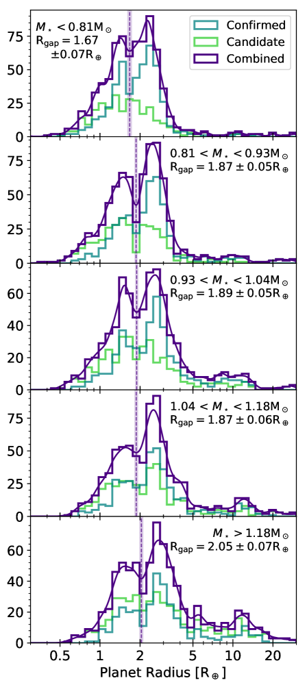
Figure 4 displays the planet radius distributions in five equally-populated stellar mass bins ranging from 0.14–2.8 $\mathrm{M_{\odot}}$. We see a clear dependence of the planet radius gap’s location in planet radius with stellar mass, increasing from 1.67 $\mathrm{R_{\oplus}}$ at $M_{\star}$ $<$ 0.81 $\mathrm{M_{\odot}}$ to 2.05 $\mathrm{R_{\oplus}}$ at $M_{\star}$ $>$ 1.18 $\mathrm{M_{\odot}}$. To quantify this dependence, we computed the gap location in planet radius and its uncertainty by (1) drawing planet radii from normal distributions centered on the expected values and with standard deviation equal to their uncertainties and (2) computing the location of the gap by finding the relative minimum between 1–4 $\mathrm{R_{\oplus}}$ in the kernel density estimate (KDE) distribution. If no gap was found, we repeated steps (1) and (2). We then computed the standard deviation for 100 successful gap samples to determine typical uncertainties in the gap location.

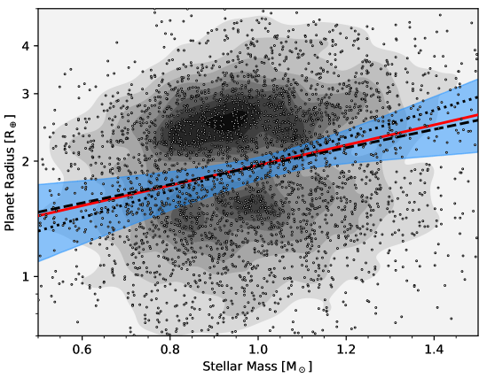
Figure 5 directly compares planet radii with stellar mass. To quantify the stellar mass dependence of the planet radius gap’s location in planet radius, we used gapfit (Loyd et al., 2020) to fit a line of the form:

$$\log_{10}{R_{\mathrm{gap}}}=m*(\log_{10}{M_{\star}/\mathrm{M}_{0}})+\log_{10}{\mathrm{R}_{0}},$$ (1)

where the average gap depth is deepest in the 2D KDE distribution (red line). To ensure gapfit found the line corresponding to the deepest valley, we constrained the range of the gapfit search to 1.5–2.4 $\mathrm{R_{\oplus}}$.

To determine the uncertainty of the best-fit line while accounting for finite sampling, we drew each of the planet radii and stellar masses from normal distributions centered at each planet radius/stellar mass value with standard deviations given by the maximum of the upper and lower uncertainties for each planet radius and stellar mass. Next, we computed a 2D KDE from these simulated observations within the bounds of Figure 5, and constructed a sample of artificial planets drawn from the 2D KDE distribution. Then, we ran gapfit with $\mathrm{M_{0}}$ = 0.95 $\mathrm{M_{\odot}}$, $\mathrm{R_{0,init}}$ = 1.89 $\mathrm{R_{\oplus}}$, $m_{init}$ = 0.27, and sig = 0.15 (bandwidth in units of $\log_{10}{\mathrm{R_{\oplus}}}$ for y-axis and $\log_{10}{\mathrm{M_{\odot}}}$ for x-axis with no covariance) with 100 bootstraps to determine the best-fit slope for the valley in the newly sampled distribution of planet radii and stellar mass. We repeated this process for 100 re-draws of the planet radii and stellar masses and then computed uncertainties from these 100 $\times$ 100 determinations of the best-fit line using the uncertainty_from_boots routine provided within gapfit. The blue shaded region in the slope in Figure 5 represents the 1$\sigma$ uncertainty region of the best-fit line ($d\log R_{\mathrm{p}}$/$d\log M_{\star}$ = 0.26${}^{+0.21}_{-0.16}$).

4.1.2 Discussion

Our results confirm the stellar mass dependence of the radius gap (Fulton & Petigura, 2018; Cloutier & Menou, 2020), with a best-fitting slope of $d\log R_{\mathrm{p}}$/$d\log M_{\star}$ = $0.26^{+0.21}_{-0.16}$. This result is consistent with the range of slopes predicted by a dependence of planet mass on stellar mass (which is required by photoevaporation models to explain the stellar mass dependence of the radius gap, Wu, 2019), and core-powered mass-loss models ($\approx$ 0.33, Gupta & Schlichting, 2020). Therefore, we are unable to differentiate between these scenarios using the valley’s slope in the planet radius-stellar mass diagram (see also Loyd et al., 2020).

To evaluate whether our inability to differentiate between core-powered mass-loss and a planet mass dependence on stellar mass in planet radius-stellar mass space is simply a problem of sample size which might be ameliorated by future discoveries, we ran Monte Carlo simulations similar to those used in Figure 5 to test various sample sizes and measurement precisions. We found that a sample size of 20,000 planets ($\approx$ 4 times the current number) assuming $typical$ planet radius and stellar mass errors of 1% is needed to reduce the uncertainties in $d\log R_{\mathrm{p}}$/$d\log M_{\star}$ to 0.04. This uncertainty would allow a 2–3$\sigma$ separation between the lower and upper bounds of a planet mass dependence on stellar mass (0.24–0.35, Wu, 2019), which contain our measured value (0.26) and the value predicted by core-powered mass-loss (0.33, Gupta & Schlichting, 2020). Even after combining all planets discovered by Kepler, $K2$ (Howell et al., 2014), and those already and to be discovered by the Transiting Exoplanet Survey Satellite ($TESS$, Ricker et al., 2014), both the sample size of $\sim$ 10,000 planets and the precision of our planet and stellar parameters would be insufficient to differentiate between photoevaporation and core-powered mass-loss in planet radius-stellar mass space.

4.2 Dependence on Stellar Age

4.2.1 Sample Selection

Figure 6: H-R diagram showing host stars colored according to their ages, as well as the marginalized distributions of stellar radii, with shaded areas representing the 16–84 percentile ranges. Purple host stars have ages greater than 1 Gyr, and green host stars have ages younger than 1 Gyr. The grey points are host stars that we do not include in our old and young samples: all evolved stars (above teal line), stars hotter than 7900 K (left of the dashed, vertical green line), and old stars with dissimilar mass, radius, and/or metallicity to the young stellar sample.

Figure 7: Radius distributions in KDE and histogram form of Kepler exoplanets with ages younger than (green) or older than (purple) 1 Gyr. The individual planet radii are plotted below as vertical ticks. The black dashed vertical line at 1.8 $\mathrm{R_{\oplus}}$ is the Fulton et al. (2017) gap radius, which separates super-Earths and sub-Neptunes. The ratio of super-Earths (1–1.8 $\mathrm{R_{\oplus}}$) to sub-Neptunes (1.8–3.5 $\mathrm{R_{\oplus}}$) significantly increases from young ages (0.61 $\pm$ 0.09) to old ages (1.00 $\pm$ 0.10).

Figure 8: Same as Figure 7 but separating the samples into high ($>$ 150 $\mathrm{F_{\oplus}}$) and low ($<$ 150 $\mathrm{F_{\oplus}}$) incident flux.

The photoevaporation and core-powered mass-loss mechanisms operate on different timescales and consequently predict different dependence of the planet radius distribution with age. Thus, we grouped planets according to the age of their host star. To ensure we only included planets with reliable properties, we removed 64 planets with radii greater than 30 $\mathrm{R_{\oplus}}$. Additionally, we removed 97 planets with grazing transits defined as $\frac{R_{\mathrm{p}}}{R_{\star}}$ + $b$ $>$ 1, where $b$, the impact parameter, is how far away from the center of the star’s disk the center of the planet transits at mid-transit (0 being at the center, and 1 being at the limb). We used $\log_{10}\frac{R_{\star}}{\mathrm{R_{\odot}}}<0.00035(T_{\mathrm{eff}}-4500)+0.15$ (similar to Equation 1 in Fulton et al., 2017) to remove giant hosts, which have a high false-positive rate (Sliski & Kipping, 2014). We also removed 1081 planets orbiting hosts without spectroscopic metallicity constraints because isochrone age estimates are metallicity-sensitive (Howes et al., 2019). After this metallicity cut, 2545 planets remained.

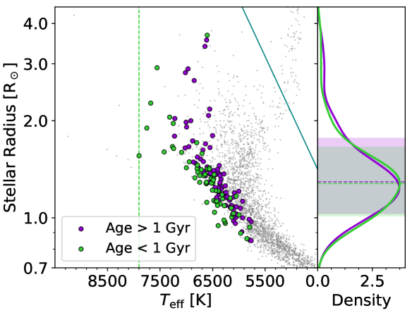
We selected 1 Gyr as our separator between young and old systems because core-powered mass-loss acts on $\sim$ Gyr timescales (Gupta & Schlichting, 2020). We could not make an age cut at 100 Myr, the timescale relevant for photoevaporation (Owen & Wu, 2017), because we have no stars with isochrone ages $<$ 100 Myr. Likewise, a cut at the age of the Hyades ($\approx$ 650 Myr, Boesgaard et al., 2016) includes too few young planets for a robust statistical comparison. We removed seven young planets with host effective temperatures hotter than 7900 K because their $T_{\mathrm{eff}}$ and masses were outliers compared to the rest of the age sample. Eighty-five planets orbit hosts with median posterior ages younger than 1 Gyr, while the remaining 2453 planets orbit hosts with median posterior ages older than 1 Gyr.

To remove degeneracies between stellar mass, age, and metallicity in the old and young planet samples, we used the NearestNeighbors function in scikit-learn (Pedregosa et al., 2011) to choose the two nearest old neighbors for every young host in stellar mass, radius, and metallicity. Because our matching function occasionally chose old neighbors such that multiple young stars are matched to the same old star, we removed any duplicate old hosts to avoid counting the same old host twice. We chose to use the two nearest neighbors instead of either one or three because the former selected fewer old planets than young planets after dropping duplicates, while the latter produced inferior stellar property-matched samples, especially in stellar mass. Our resulting property-matched sample included 90 old planets. In addition to removing stellar population biases, this careful sample selection also reduced potential detection biases for small planets between the old and young samples, all while retaining the full young planet sample. We used K-S tests to compare the stellar mass, radius, and metallicity distributions of the old and young samples, producing p-values of 0.24, 0.58, and 0.997, respectively, confirming the distributions are statistically similar. Figure 6 shows an H-R diagram of the host star sample after making the above cuts, separated by the relevant age bins. We flag these planets as “Old” and “Young” in Table 1.

4.2.2 Results

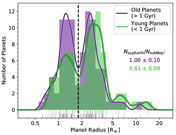
Figure 7 shows the planet radius distributions of the old and young planet samples. We observe that the gap occurs at approximately the same planet radius in both the old and young planet distributions. Remarkably, we also observe that the ratio of super-Earths compared to sub-Neptunes significantly increases from young to old stellar ages.

To quantify this age dependence, we computed the uncertainties in the ratio of super-Earths to sub-Neptunes using Monte Carlo simulations to draw each old and young planet radius from a normal distribution given its measured value and uncertainty. We define super-Earths as planets between 1–1.8 $\mathrm{R_{\oplus}}$, and sub-Neptunes as planets between 1.8–3.5 $\mathrm{R_{\oplus}}$ (Fulton et al., 2017). We then counted the number of super-Earths and sub-Neptunes, repeated this process 1000 times for both the old and the young distributions and then computed the standard deviation of the ratios of super-Earths to sub-Neptunes.

Our data show a significant increase in the fraction of super-Earths as a function of age, with the fraction of super-Earths to sub-Neptunes increasing from 0.61 $\pm$ 0.09 at young ages ($<$ 1 Gyr) to 1.00 $\pm$ 0.10 at old ages ($>$ 1 Gyr). This result is insensitive to the choice of impact parameter cut ($\gtrsim$ 2$\sigma$ for $b$ $<$ 0.7–0.9), gap location ($\gtrsim$ 3$\sigma$ for 1.9–2.0 $\mathrm{R_{\oplus}}$), and radius range used to define super-Earths and sub-Neptunes ($\gtrsim$ 4$\sigma$ for 0.8–1.8 $\mathrm{R_{\oplus}}$ and 1.8–5 $\mathrm{R_{\oplus}}$, respectively). Similarly, if we instead used 1533 old planets hosted by old stars larger than 0.9 $\mathrm{R_{\odot}}$ rather than the property-matched sample described in the previous section, we computed a $\gtrsim$ 3$\sigma$ difference in the ratios of young and old super-Earths to sub-Neptunes. Reassuringly, Fulton et al. (2017) computes the $occurrence$ ratio of super-Earths to sub-Neptunes for the entire planet sample to be 0.8 $\pm$ 0.2, approximately the average of our old and young ratios.

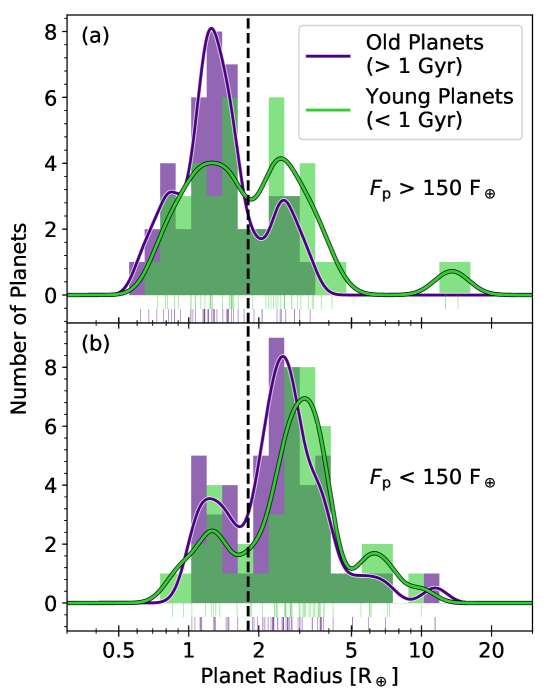
We also compared the low ($F_{\mathrm{p}}$ $<$ 150 $\mathrm{F_{\oplus}}$) and high ($F_{\mathrm{p}}$ $>$ 150 $\mathrm{F_{\oplus}}$) flux planet radius distributions for old and young exoplanets (Figure 8). We chose 150 $\mathrm{F_{\oplus}}$ because it splits the young sample of planets almost in half: 41 young and 41 old planets receive more than 150 $\mathrm{F_{\oplus}}$ and 44 young and 49 old planets receive less than 150 $\mathrm{F_{\oplus}}$. Interestingly, we observe stark differences between old and young planets. At high incident flux (Figure 8(a)), we observe a large difference between the young and old planet radius distributions. We compute the ratios of super-Earths to sub-Neptunes to be 1.00 and 2.67 for the young and old planets, respectively. However, at low incident flux (Figure 8(b)), the overall distributions do not show a strong difference as a function of age, with tentative evidence that old sub-Neptunes are smaller than young sub-Neptunes. We ran K-S tests to quantitatively compare the old and young distributions in both panels, and found they were statistically distinguishable in the top panel (p-value = 0.02) and indistinguishable in the bottom panel (p-value = 0.11).

Figure 9: Single transit signal-to-noise ratios (SNR) for an Earth-size planet with a three-hour transit duration orbiting each individual planet host used in Figures 6–8 (large circles) and Kepler target star (dots). Larger values on this plot indicate that planets are easier to detect. We use the CDPP3 values from Christiansen et al. (2012) and Equation B2 in Petigura et al. (2018) to compute the SNR.

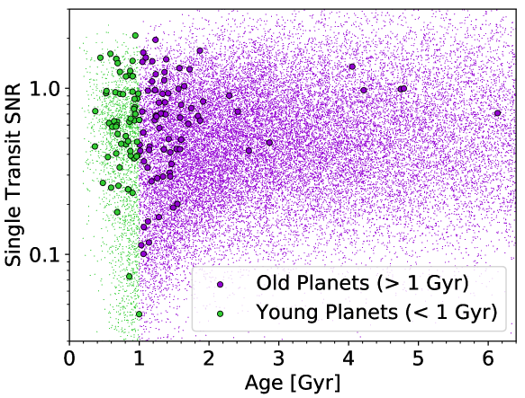
A potential bias in our results is the sensitivity of planet detection to stellar age. This is because young stars are typically noisier due to their increased activity (Skumanich, 1972) and thus smaller planets might not be detected around them. To test this, we evaluated the CDPP3 values (Christiansen et al., 2012) to determine the single transit signal-to-noise ratio (SNR) for an Earth-size planet with a three hour transit duration (as in Petigura et al., 2018) for each host star in Figure 9. This comparison also accounts for differences in the stellar radius distributions, although we control for these differences in our sample selection.

We find that the young planets typically have similar SNR compared to the old planets, and hence are just as difficult to detect. The large scatter of points in Figure 9 dominate what would be small differences in the old and young median single transit SNR values. Similarly, when we compare the median single transit SNR values the overall Kepler sample with cuts similar to those in Figure 6, we find no significant difference between the old median SNR ($\approx$ 0.43) and young median SNR ($\approx$ 0.40), given the large point-by-point scatter. Therefore, we conclude that our results are robust against a planet detection bias with stellar age.

Another bias that could affect our results is the presence of undetected binary companions, which would cause stars to be incorrectly assigned old ages. While we have removed most wide binaries using Gaia and de-biased stellar photometry for binary contamination (1), it is inevitable that some close binaries will contaminate our old and young samples. After removing all AO-detected companions (Furlan et al., 2017), the young and old distributions in Figure 7 remain mostly unchanged. However, the distributions in Figure 8(a) are sensitive to the removal of AO-detected binaries, as binaries make stars appear more luminous and increase the apparent irradiance of the planets.

To test the potential for binaries to bias our results, we estimated the number of planets that may have been mistakenly placed in the older sample because of binary contamination. We adopted a typical binary mass ratio ($M_{\mathrm{prim}}/M_{\mathrm{sec}}$ $\approx$ 0.5) and binary fraction for solar-type stars ($F_{\mathrm{bin}}$ $\approx$ 40%) determined in Raghavan et al. (2010) and Moe & Di Stefano (2017). We also used the +50% isochrone age bias determined from the 1.15 $\mathrm{M_{\odot}}$ star in Figure 4 of 1. Using these assumptions, we predict that 55 planets $\times$ $F_{\mathrm{bin}}$ $\approx$ 22 planets are orbiting stars with isochrone ages between 1–1.5 Gyr that should be younger than 1 Gyr due to binary contamination. We then shifted these 22 planets into the young distribution assuming (1) they mimic the old distribution’s ratio of super-Earths to sub-Neptunes and (2) their measured radii are not affected significantly by binary contamination. Consequently, we computed a 0.76 $\pm$ 0.09 ratio of super-Earths to sub-Neptunes for the young planet distribution. Comparing this to the 1.00 $\pm$ 0.10 ratio of super-Earths to sub-Neptunes for the old planet distribution, we still arrive at a $>$ 2$\sigma$ difference between the old and young distributions. Given our conservative assumptions, we conclude that undetected stellar companions will not significantly affect our results on the age dependence of the radius valley.

4.2.3 Discussion

Figure 7 suggests that sub-Neptunes evolve to become super-Earths over Gyr timescales. This is consistent with the core-powered mass-loss mechanism (Gupta & Schlichting, 2020), which predicts that the transition of sub-Neptunes to super-Earths occurs over Gyr timescales as the planets gradually lose their atmospheric envelopes due to their heated cores. While our result supports the core-powered mass-loss mechanism, it does not rule out the possibility that photoevaporation is also acting on the observed planet population. Given that photoevaporation is expected to occur in the first $\sim$ 100 Myr (Owen & Wu, 2017; Wu, 2019) of a planet’s lifetime and our 100 Myr minimum grid age (1), we are mostly insensitive to any planetary evolution before 100 Myr ages, barring extreme planet radius evolution during that time. Our Monte Carlo simulations do not account for the uncertainties in the stellar ages and hence it is likely that there is contamination between the old and young planets. However, given the magnitude of the errors and the difference in the number of old and young stars in our sample, it is more likely that older stars are contaminating the younger bins (Eddington bias). If this bias truly exists in our sample, any observed differences between the old and young samples will be reduced by this bias, thus the true difference between young and old planets is greater.

Our result agrees with Berger et al. (2018a), who used lithium abundances relative to the Hyades to separate young (A(Li)_⋆ $>$ A(Li)_Hyades) and old (A(Li)_⋆ $<$ A(Li)_Hyades) planets. In particular, Berger et al. (2018a) find that there is a significant difference in the sizes of planets in the old and young planet radius histograms and that young planets are larger. This result was tentative ($\approx$ 2–3$\sigma$) due to the small sample size of the young planets as compared to the old planets. Although Berger et al. (2018a) does not explicitly quantify the number of super-Earths and sub-Neptunes, the largest difference between their old and young samples occurs at $\gtrsim$ 2 $\mathrm{R_{\oplus}}$, where the number of sub-Neptunes in the young sample is significantly greater than the number sub-Neptunes in the old sample.

Our observation of a similar gap radius for young and old planets is expected, as we carefully chose stellar samples with similar stellar mass, which should produce a gap at a similar location in the distribution of planet radii (§4.1). While core-powered mass-loss predicts that the gap’s location should increase slightly to larger radii in the first $\sim$ Gyr (Gupta & Schlichting, 2020), such behavior will be hard to definitively establish given typical uncertainties on stellar age, mass, and planet radius. Meanwhile, photoevaporation does not predict significant gap movement after the first $\sim$ 100 Myr (Owen & Wu, 2016, 2017).

We interpret that the differences between the old and young distributions as a function of incident flux in Figure 8 are consistent with core-powered mass-loss, which predicts that planets that receive higher incident fluxes may experience increased and potential runaway mass-loss over timescales of $\sim$ Gyr due to increased equilibrium temperatures at the Bondi radius (Ginzburg et al., 2016, 2018; Gupta & Schlichting, 2019, 2020). Conversely, sub-Neptunes that receive low incident fluxes (Figure 8(b)) will simply cool and contract, shifting from the larger radii ($\approx$ 3 $\mathrm{R_{\oplus}}$) at young ages to the smaller radii ($\approx$ 2.5 $\mathrm{R_{\oplus}}$) at old ages. This is predicted by photoevaporation as well (Lopez et al., 2012; Owen & Wu, 2017), but it cannot describe the difference in high incident flux distributions over Gyr timescales. we caution that these inferences are tentative, especially because of the small number of planets contained in the old and young low flux (49 and 44 planets, respectively) and old and young high flux (41 and 41 planets, respectively) distributions. Additionally, both the young and the old low flux planet radius distributions are likely biased more significantly by selection effects than the high flux distributions, as small planets at low incident fluxes are more difficult to detect.

4.3 Planets Within the Gap

According to photoevaporation, which produces radius changes within the first 100 Myr of a host’s lifetime (Owen & Wu, 2017), we should not see any planets within the gap (Van Eylen et al., 2018) at old ages. Conversely, the $\sim$ Gyr timescales of core-powered mass-loss (Gupta & Schlichting, 2020) suggest that we should find a few planets in the gap region as they transition from sub-Neptunes to super-Earths. It is currently unclear whether any planets firmly exist within the radius valley. Large population studies have revealed that there are at least a few planets that fall within the planet radius gap (Berger et al., 2018b; Fulton & Petigura, 2018), although smaller, more precise planet samples have revealed a complete lack of planets within the gap (Van Eylen et al., 2018).

To investigate this, we used gapfit (Loyd et al., 2020) to determine the best-fit parameters in the planet radius-incident flux diagram using:

$$\log_{10}{R_{\mathrm{gap}}}=m*(\log_{10}{F_{\mathrm{p}}/\mathrm{F}_{0}})+\log_{10}{\mathrm{R}_{0}},$$ (2)

assuming a pivot point $\mathrm{F}_{0}$ = 100 $\mathrm{F_{\oplus}}$ and the optimal Gaussian kernel width sig = 0.15 (gapfit, Loyd et al., 2020). We found $m$ = $d\log R_{\mathrm{p}}$/$d\log F_{\mathrm{p}}$ = 0.057 and $\mathrm{R}_{0}$ = 1.86 $\mathrm{R_{\oplus}}$. Next, we computed parallel lines by varying the $\mathrm{R}_{0}$ parameter by typical uncertainties ($\pm$ 0.09 $\mathrm{R_{\oplus}}$) determined from a combination of Monte Carlo and bootstrap simulations, ignoring uncertainties in the slope. We then isolated all confirmed planets that were within the log-log lines with slopes, $m$ = $d\log R_{\mathrm{p}}$/$d\log F_{\mathrm{p}}$ = 0.057, and pivot point central gap radii, $\mathrm{R}_{0}$ = 1.77 and 1.95 $\mathrm{R_{\oplus}}$. We also removed all planets with 1$\sigma$ errors in planet radius that would place them outside the log-log lines representing bounds of the planet radius gap as a function of incident flux.

Following these cuts, five planets remain in the gap: Kepler-11 b, Kepler-110 b, Kepler-114 c, Kepler-634 b, and Kepler-887 b. We conclude that these five planets may currently undergo core-powered mass-loss, but caution that they are only $\sim$ 1$\sigma$ removed from the gap boundaries. Additional follow-up observations will be required to definitively identify planets inside the radius valley.

5 The Hot Sub-Neptunian Desert

Figure 10: Stellar age (panel (a)) and mass (panel (b)) distributions for planets with high incident flux ($F_{\mathrm{p}}$ $>$ 650 $\mathrm{F_{\oplus}}$) within the hot sub-Neptunian desert $R_{\mathrm{p}}$ = 2.2–3.8 $\mathrm{R_{\oplus}}$ (red), at high incident flux outside the hot sub-Neptunian desert (blue), and the overall Kepler target sample with reliable ages (RUWE $<$ 1.2, iso_gof $>$ 0.99, and TAMS $<$ 20 Gyr, black). The blue and red ticks represent the individual ages/masses used to calculate the KDEs using bandwidths following Scott’s Rule (Scott, 1992). The dashed vertical lines and shaded areas are the median and 1$\sigma$ bounds.

Figure 11: Panel (a): Planet radius versus incident flux for Kepler exoplanets in the hot sub-Neptunian desert (red) defined by Lundkvist et al. (2016), at incident fluxes $>$ 650 $\mathrm{F_{\oplus}}$ and outside the desert (blue), and at incident fluxes $<$ 650 $\mathrm{F_{\oplus}}$(grey). Solid and translucent points are confirmed and candidate planets, respectively. The black, butted bars show the incident flux history of each planet, starting at the incident flux the planet received at the zero age main sequence (ZAMS). Panel (b): Current divided by ZAMS flux ratio for desert planets (red), other high incident flux planets (blue), and all other planets (grey).

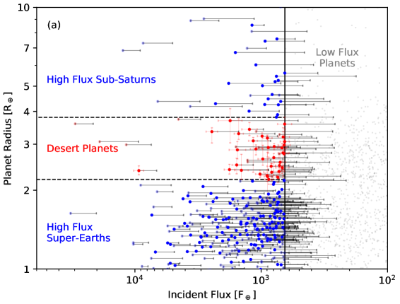
The hot sub-Neptunian desert, defined as $R_{\mathrm{p}}$ = 2.2–3.8 $\mathrm{R_{\oplus}}$ and $F_{\mathrm{p}}$ $>$ 650 $\mathrm{F_{\oplus}}$, is another region of parameter space believed to be devoid of planets (Lundkvist et al., 2016). The lack of planets in the hot sub-Neptunian desert can be explained by photoevaporation (Lopez et al., 2012; Owen & Wu, 2016, 2017), with hydrogen and helium atmospheres being completely lost to the large EUV flux at small orbital separations (Lopez, 2017). At lower incident EUV fluxes, planets still lose significant portions of their atmospheres, but stabilize at an envelope mass fraction of 1–2% (Owen & Wu, 2017). Berger et al. (2018b) found 74 confirmed planets/planet candidates in the “desert”, and suggested that some of these planets (1) may be the remnants of the photoevaporation of a giant planet’s envelope (Baraffe et al., 2005), (2) did not receive enough EUV flux to lose their low molecular weight atmospheres (Owen & Wu, 2017), or (3) may have high molecular weight atmospheres (Lopez, 2017). Our newly derived stellar masses and ages can shed additional light on the properties and formation of this intriguing class of planets.

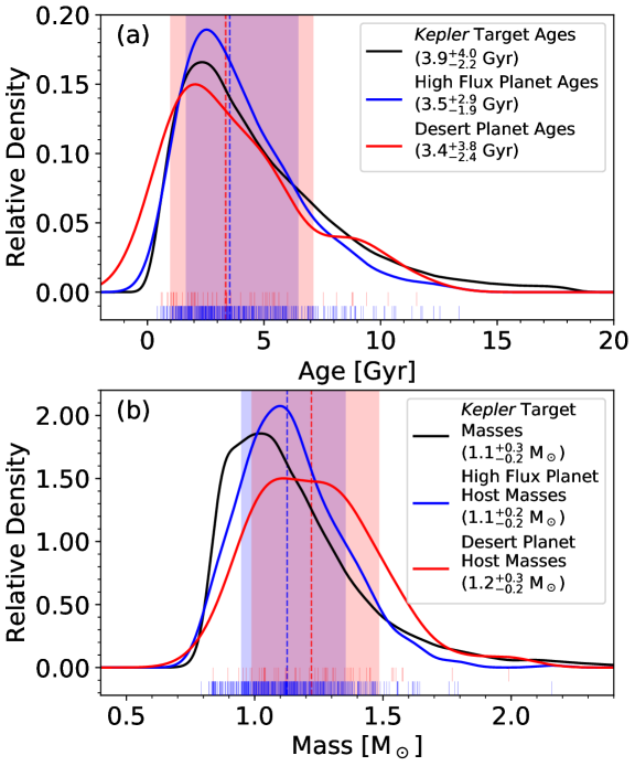
Figure 10(a) shows the age distribution of planets within (red) and outside (blue) the hot sub-Neptunian desert at high incident fluxes ($>$ 650 $\mathrm{F_{\oplus}}$, Lundkvist et al., 2016). We also plot the overall Kepler sample for comparison. We observe similar stellar age distributions for planets within the hot sub-Neptunian desert and those at high incident fluxes with radii outside 2.2–3.8 $\mathrm{R_{\oplus}}$. The median ages and distributions are almost identical, which is also confirmed with a K-S test (p-value = 0.14). We therefore conclude that most of these “desert dwellers” are not young planets that are currently losing mass.

Unlike stellar ages, Figure 10(b) indicates a difference between the stellar mass distributions of high incident flux planets inside and outside the desert. A K-S test yielded a p-value of 0.02, indicating a difference at $\approx$ 2$\sigma$ significance. Therefore, we tentatively conclude that desert planets tend to be around more massive stars. This conclusion is also supported by a K-S test using host star radii and uncertainties, yielding a p-value of 0.007. Because hot sub-Neptune planet hosts appear to have higher stellar masses and larger stellar radii, we hypothesize that these planets could have shifted into the desert through stellar evolution.

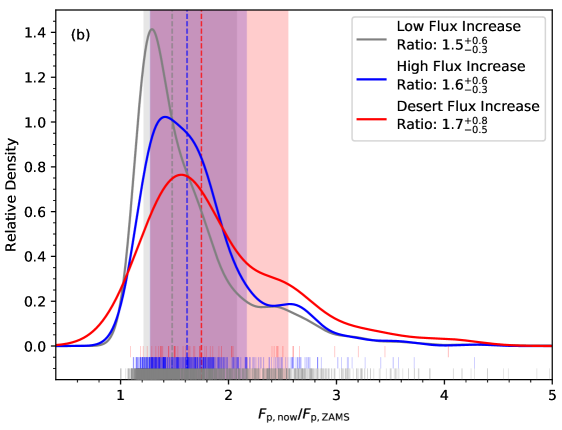
To investigate this, Figure 11(a) shows the incident flux history of planets within and outside the desert. We count 35 confirmed and 15 planet candidates within the hot sub-Neptunian desert (as defined by Lundkvist et al., 2016), and we denote them with the “Desert” flag in Table 1. Figure 11(b) shows the ratios of the current flux compared to ZAMS flux (see Table 1 for planets in the different regimes of panel (a). Together, Figures 11(a) and (b) suggest that 60% of desert planets have moved into the desert as a result of stellar luminosity evolution. Therefore, we infer that the majority of desert planets were not, in the first $\sim$ 100 Myr, exposed to enough EUV flux to completely strip their atmospheres. However, this incident flux evolution does not explain all desert planets.

We find nine confirmed planets within the desert by $>$ 1$\sigma$ even after accounting for the effects of stellar evolution on the incident flux: Kepler-234 b, Kepler-541 b, Kepler-611 b, Kepler-644 b, Kepler-645 b, Kepler-656 b, Kepler-1016 b, Kepler-1171 b, and Kepler-1518 b. If we assume a ZAMS luminosity that corresponds to the ZAMS luminosity of the lower mass uncertainty bound for each system, we still find three planets within the desert: Kepler-644 b, Kepler-645 b, and Kepler-1171 b. Kepler-644 and Kepler-645 have AO-detected companions, and thus their stellar properties are likely inaccurate, in addition to the incident fluxes their planets receive. Using ZAMS luminosities corresponding to the lower mass uncertainty bound is a pessimistic assumption, which overestimates the increase in the star’s luminosity since the ZAMS and accounts for uncertainties. Given 100 Myr H/He atmosphere-loss timescales (Owen & Wu, 2017), it is unlikely that these desert-dwelling planets are typical sub-Neptune-mass planets with H/He envelopes, unless they migrated to their current orbital separations (Dong et al., 2018) and/or have higher-molecular weight atmospheres (Lopez, 2017; Gaidos et al., 2020). It is also possible that these planets are the bare cores of 2–3$\times$ more massive planets (Armstrong et al., 2020). While photoevaporation is not expected to strip enough atmospheric mass off of these massive cores, tidal disruption (Vick et al., 2019) or giant planet collisions (Mordasini, 2018) can produce the required mass loss. Alternatively, these bare cores may form in-situ by opening up a gas-less gap in the protoplanetary disk and avoiding runaway accretion (Lee, 2019). Ultimately, these desert-dwellers represent interesting tests of planet formation and evolution theories, and warrant additional scrutiny.

6 Cool Planets

6.1 Cool, Inflated Jupiters

Figure 12: Radius versus incident flux for Kepler’s cool Jupiters. Planets are colored by isochrone age. Orange squares and red rings indicate stars that are rotating more rapidly or exhibit more UV-excess compared to the Hyades, respectively. Grey points are candidate planets. The red curve represents the maximum radius for a 4.5 Gyr, Jupiter-mass, pure hydrogen and helium object (Thorngren et al., 2016). The inset shows the position of the host stars on the H-R diagram compared to the Kepler target sample (grey).

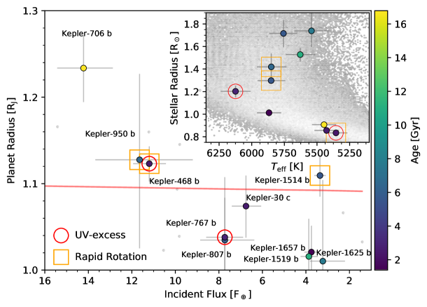
The mechanism producing the inflated radii of hot Jupiters is still a major unsolved problem (Guillot & Showman, 2002; Fortney & Nettelmann, 2010; Fortney et al., 2011; Baraffe et al., 2010, 2014; Laughlin & Lissauer, 2015; Laughlin, 2018; Komacek et al., 2020). Most theories are linked to the observation that all inflated Jupiters experience high incident flux (Demory & Seager, 2011; Laughlin et al., 2011; Miller & Fortney, 2011), whether they are orbiting main sequence stars or have been re-inflated from the effects of post-main sequence stellar evolution (Lopez & Fortney, 2016; Grunblatt et al., 2016, 2017, 2019). Thus, finding examples of cool, inflated Jupiters may present an interesting challenge to these theories. Berger et al. (2018b) identified three Jupiters with anomalously large radii and at $<$ 150 $\mathrm{F_{\oplus}}$. If these planets are inflated at low incident fluxes, there must be some other mechanism causing their inflation. For example, these planets may be young and hot from the gravitational energy of accretion, and this additional energy could produce an inflated atmosphere (Lopez et al., 2012). These cool, inflated Jupiters could also be heated from recent tidal interactions with other planets and their host star (Jackson et al., 2008; Fortney et al., 2010).

Similar to Berger et al. (2018b), we find a small sample of cool, confirmed (or validated), $>$ 1 $\mathrm{R_{J}}$ Jupiters (Figure 12). In addition to isochrone ages, we mark points according to whether they exhibit UV-excess (red circle) or rapid rotation (orange square) as additional indicators for youth. We flag a star as having UV-excess when it meets two criteria: (1) $m_{\mathrm{NUV}}-m_{K_{s}}<8.3$ (to avoid magnitude-limited cases) and (2) $m_{\mathrm{NUV}}-m_{K_{s}}<m_{\mathrm{NUV}}(M_{K_{s}})_{\mathrm{Hyades}}-m_{K_{s}}(M_{K_{s}})_{\mathrm{Hyades}}$, where the condition is set by the Hyades relation evaluated at the $M_{K_{s}}$ of the Kepler star. The Hyades cluster ($\sim$ 650 Myr Boesgaard et al., 2016) has a well-defined trend in NUV–$K_{s}$ versus $M_{K_{s}}$, making it an effective separator for young/old stars in the Kepler field (Berger et al., 2018a). We obtained the NUV fluxes for the Kepler and Hyades stars from the Galaxy Evolution Explorer (GALEX; Martin et al., 2005; Olmedo et al., 2015). Similarly, we flag a star as having rapid rotation if its rotation period is more rapid than the Hyades gyrochrone with an initial rotation period of 3.4 days (Kundert et al., 2012). We use the rotation periods derived in McQuillan et al. (2013, 2014) or Mazeh et al. (2015).

We find two planets that are significantly above the maximum radius for a 4.5 Gyr, Jupiter-mass, pure hydrogen and helium object (Thorngren et al., 2016). Kepler-468 b appears to be young according to its host’s isochrone age (2.4${}^{+3.3}_{-1.7}$ Gyr), excess UV flux (Skumanich, 1972; Soderblom, 2010), and rapid rotation period. It does not have a rotation period detection according to McQuillan et al. (2013, 2014) or Mazeh et al. (2015), but an inspection of the Kepler lightcurve reveals a rotation period of $\approx$ 5.7 days, consistent with a young age (Barnes & Kim, 2010). Kepler-468 has RUWE = 1.15, which is below the threshold for being a likely binary. Similarly, Kepler-468 does not appear to have any companions according to the high resolution imaging (Law et al., 2014; Furlan et al., 2017). Even at 2.4 Gyr, a Jupiter-mass planet may still be cooling and contracting from its heat from formation, although the majority of this contraction occurs within the first $\sim$ Gyr (Fortney et al., 2007; Linder et al., 2019). Hence, it is possible that Kepler-468 b is young and still cooling and contracting from its heat from formation.

Unlike Kepler-468 b, Kepler-706 b does not appear to orbit a young star. Kepler-706 has an isochrone age of $\sim$ 17 Gyr, a rotation period of $\approx$ 38 days measured from the Kepler lightcurve, and a NUV magnitude that is beyond the GALEX limiting magnitude of 22.6 (Olmedo et al., 2015). While the isochrone age is unreliable, the rotation period supports an old age for this star (Barnes & Kim, 2010). Furthermore, neither the RUWE value (1.13) nor high resolution imaging from Law et al. (2014) indicate the presence of a stellar companion.

If confirmed, the radius and age of Kepler-706 b would be highly interesting. Given its old age, it is very unlikely that it is inflated from its residual heat from formation based on the expected cooling timescales (Lopez et al., 2012). Kepler-706 b orbits every 41 days, so it is also unlikely that its radius is inflated by strong tidal or magnetic interactions with its host star, barring a highly elliptical orbit. Planet-planet interactions typically produce only a fraction of the tidal heating that is caused by the host star (Hay & Matsuyama, 2019), but this heating is strongly dependent on the proximity and the mass of the other planet. Rings are another potential explanation for Kepler-706 b’s inflated radius (Schlichting & Chang, 2011), but we cannot confirm the presence of rings with Kepler’s lightcurve cadence/precision. Additional follow-up observations will be required to confirm whether Kepler-706 b is indeed a bona-fide cool, inflated Jupiter.

6.2 Habitable Zone Planets

Our work also yields a revised list of planets in the habitable zone. Following the definition of Kane et al. (2016), we find 133 planet candidates and 32 confirmed planets within the habitable zone (0.25–1.5 $\mathrm{F_{\oplus}}$), all of which are flagged in Table 1. Compared to Berger et al. (2018b), we count two fewer confirmed and 24 more candidate planets. We report eight confirmed planets with radii $<$ 2 $\mathrm{R_{\oplus}}$: Kepler-62 e, Kepler-62 f, Kepler-186 f, Kepler-283 c, Kepler-440 b, Kepler-442 b, Kepler-452 b (but see also Mullally et al., 2018), and Kepler-1544 b, although Kepler-62, Kepler-186, and Kepler-283 have AO-detected companions (Furlan et al., 2017). This increase of habitable zone candidate planets is mostly caused by the slightly cooler $T_{\mathrm{eff}}$ derived in 1, which produce smaller incident fluxes for planets at the same orbital periods.

7 Single and Multi Planet Systems

Figure 13: Cumulative age distribution functions (CDFs) of Kepler systems with multiple transiting planets (red, 539 systems) and one transiting planet (blue, 1768 systems).

Several observational results suggest that the Kepler multiplanet systems (multis) have smaller eccentricities and inclinations than the Kepler systems with just one small transiting planet (singles). The Kepler multis are nearly coplanar (Fang & Margot, 2012; Fabrycky et al., 2014), with a typical mutual inclination of $1.0^{\circ}$-$2.2^{\circ}$. These typical mutual inclinations are smaller than what is required for all of the planets to transit, indicating that detection bias alone cannot explain the observed coplanarity of the Kepler multis. Furthermore, the Kepler singles have higher eccentricities than the multis, as determined from their more varied transit durations (Xie et al., 2016; Mills et al., 2019; Van Eylen et al., 2019). In multis with an ultra-short period planet, the mutual inclinations between the planets are higher than in multis without an ultra-short period planet (Dai et al., 2019), suggesting that the evolutionary pathway that creates ultra-short period planets also excites planetary inclinations and eccentricities (e.g., Petrovich et al., 2019).

What physical processes affect the ecccentricities and inclinations of the Kepler planets? The host star masses, metallicities, and $v\sin{i}$’s of the Kepler singles and multis are statistically indistinguishable (Weiss et al., 2018), suggesting that the host stars are not the main source of the observed differences in the eccentricity and inclination distributions. One possible source of dynamical excitation (and also instability) is the planets themselves: dynamically packed planetary systems become unstable on timescales of $10^{7}$-$10^{10}$ orbits (Obertas et al., 2017), with the closest-packed systems typically becoming unstable earliest. Systems with larger eccentricities are more likely to become unstable, excited in inclination, and tidally circularized (Pu & Lai, 2019; Petrovich et al., 2019). Long-distance processes such as a gravitational perturbation from a passing star or can also affect the coplanarity and stability of the Kepler multis (Spalding & Batygin, 2016). The likelihood that any of these disruptive mechanisms has already occurred increases with time. Therefore, significant differences in stellar age between the single and multi-planet systems, in particular a preference for single planets to be around older stars, may point to an evolutionary pathway from the multis to the singles.

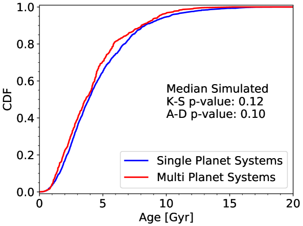
Figure 13 shows cumulative distribution functions for ages of multis (red, 539 systems) and singles (blue, 1768 systems). We observe that the single transiting planet systems indeed appear to be on average older than the multiple transiting planet systems. To quantify the difference of these two distributions, we conducted Monte Carlo K-S simulations to account for individual errors in the ages of our stars. We also performed Monte Carlo Anderson-Darling (A-D, scipy’s anderson_ksamp; Scholz & Stephens, 1987; Virtanen et al., 2020) test simulations in a similar manner. The resulting p-values are 0.12 and 0.10 for the K-S and A-D tests, respectively, indicating that the single- and multi-planet ages are statistically indistinguishable. Requiring spectroscopic metallicities for single and multi systems, which improve isochrone ages (Howes et al., 2019), produced p-values of 0.59 and 0.25 (capped) for the K-S and A-D tests, respectively.

We therefore conclude that the ages of single and multiple transiting planet systems are statistically indistinguishable within the precision of our age measurements. This implies that dynamical interactions that affect planet eccentricities and inclinations such as planet-planet and planet-passing star interactions operate significantly faster than the $\sim$ Gyr timescales that can be resolved by our sample (e.g., Spalding & Batygin, 2016; Obertas et al., 2017), and may happen at almost any age. For instance, young singles could be the multis that were disrupted at young ages, while old multis have not been disrupted yet.

8 Summary and Conclusions

We presented a re-analysis of Kepler exoplanet properties using the uniform stellar properties provided by 1. In particular, we performed a systematic analysis of planet properties as a function of stellar mass and age for the entire Kepler sample. Our main conclusions are as follows:

• We observe that the location of the planet radius gap increases in planet radius with increasing stellar mass, with a slope of $d\log R_{\mathrm{p}}$/$d\log M_{\star}$ = $0.26^{+0.21}_{-0.16}$, consistent with previous results based on smaller samples by Fulton & Petigura (2018) and Cloutier & Menou (2020). The uncertainty on the slope even for the full Kepler sample is too large to discern between a planet mass dependence on stellar mass (as required by photoevaporation, Wu, 2019) and core-powered mass-loss (Gupta & Schlichting, 2020). We estimate that differentiating between these theories would require $\gtrsim$ 20,000 planets with 1% fractional precisions in planet radius and stellar mass.

• We find first evidence for a stellar age dependence of the fraction of super-Earths to sub-Neptunes, increasing from young planets ($<$ 1 Gyr, 0.61 $\pm$ 0.09) to old planets ($>$ 1 Gyr, 1.00 $\pm$ 0.10). This is consistent with predictions of the core-powered mass-loss mechanism that sub-Neptunes evolve to become super-Earths over Gyr timescales (Gupta & Schlichting, 2020), but we caution that our sample does not constrain evolution at times $\lesssim$ 100 Myr due to photoevaporation (Owen & Wu, 2017). We also observe that the age dependence of the fraction of super-Earths to sub-Neptunes becomes stronger with higher incident flux. . However, we caution that the latter results may be influenced by small number statistics and possible effects of undetected binary companions.

• We identify 35 confirmed planets and 15 planet candidates that occupy the hot sub-Neptunian desert (Lundkvist et al., 2016). We determine that most of the desert planets orbit evolved stars, and thus it is unlikely that they are young planets currently undergoing mass loss. In addition, we identify nine planets that are within the desert even after accounting for stellar evolution: Kepler-234 b, Kepler-541 b, Kepler-611 b, Kepler-644 b, Kepler-645 b, Kepler-656 b, Kepler-1016 b, Kepler-1171 b, and Kepler-1518 b.

• We investigate Kepler’s population of cool ($F_{\mathrm{p}}$ $<$ 20 $\mathrm{F_{\oplus}}$) Jupiters, and identify Kepler-706 b and Kepler-468 b as candidates for cool, inflated Jupiters. While Kepler-468 b orbits a young star and is potentially inflated due to its heat from formation, Kepler-706 b apparently orbits an old star based on its rotation period. Future observations will be required to rule out binary companions that could bias the radius measurement.

• We find that 32 confirmed and 133 planet candidates have incident fluxes from 0.25–1.50 $\mathrm{F_{\oplus}}$ and thus occupy a nominal habitable zone (Kane et al., 2016). Of these, 37 planet candidates and eight confirmed planets have radii smaller than 2 $\mathrm{R_{\oplus}}$(but see also Mullally et al., 2018; Burke et al., 2019): Kepler-62 e, Kepler-62 f, Kepler-186 f, Kepler-283 c, Kepler-440 b, Kepler-442 b, Kepler-452 b, and Kepler-1544 b.

• We find that stars hosting multiple transiting planets have ages that are on average higher but are statistically indistinguishable from those of single planet host stars. This implies that if dynamical interactions (planet-planet and/or planet-passing star interactions) frequently scatter planets out of our line-of-sight to produce single transiting planet systems, these interactions are quick (e.g., Spalding & Batygin, 2016; Obertas et al., 2017) and may happen over a wide range of ages.

Our results demonstrate the importance of precise, homogeneous parameters and the power of stellar ages and masses to allow a more comprehensive investigation of exoplanet populations and their evolution over time. An extension to lower mass stars will require the use of alternative age indicators such as lithium abundances, rotation, and UV-excess measurements to identify a more robust sample of young Kepler hosts. Additionally, a homogeneous stellar classification of planet hosts observed by $K2$ and $TESS$ will offer new insights into their planet populations and provide additional clues about planet formation and evolution.

Table 1: Planet Parameters

KIC ID	KOI ID	Planet Disposition	Planet Radius [$\mathrm{R_{\oplus}}$]	Semimajor Axis [AU]	Incident Flux [$\mathrm{F_{\oplus}}$]	ZAMS Flux [$\mathrm{F_{\oplus}}$]	Interesting Object Flag
11446443	1.01	CONFIRMED	14.21${}^{+0.29}_{-0.29}$	0.0355${}^{+0.0008}_{-0.0008}$	854.78${}^{+69.34}_{-64.81}$	524.75	AO
10666592	2.01	CONFIRMED	16.45${}^{+0.35}_{-0.34}$	0.0381${}^{+0.0005}_{-0.0006}$	4285.95${}^{+331.23}_{-336.99}$	2394.68	AO
10748390	3.01	CONFIRMED	4.88${}^{+0.08}_{-0.07}$	0.0516${}^{+0.0006}_{-0.0004}$	86.58${}^{+5.24}_{-4.73}$	58.22
3861595	4.01	CONFIRMED	13.18${}^{+0.42}_{-0.82}$	0.0583${}^{+0.0007}_{-0.0015}$	5244.42${}^{+478.90}_{-520.46}$	3647.63	AO
11853905	7.01	CONFIRMED	4.01${}^{+0.10}_{-0.10}$	0.0455${}^{+0.0007}_{-0.0010}$	1247.17${}^{+99.09}_{-99.02}$	719.80
6922244	10.01	CONFIRMED	15.53${}^{+0.36}_{-0.36}$	0.0490${}^{+0.0007}_{-0.0008}$	1482.86${}^{+117.24}_{-126.09}$	965.36	AO
5812701	12.01	CONFIRMED	14.36${}^{+0.32}_{-0.29}$	0.1509${}^{+0.0018}_{-0.0021}$	204.64${}^{+18.91}_{-15.30}$	141.77	YoungAO
10874614	17.01	CONFIRMED	12.76${}^{+0.27}_{-0.32}$	0.0445${}^{+0.0007}_{-0.0009}$	793.33${}^{+56.16}_{-61.47}$	450.14
8191672	18.01	CONFIRMED	14.91${}^{+0.43}_{-0.42}$	0.0504${}^{+0.0008}_{-0.0007}$	1826.02${}^{+162.50}_{-151.51}$	1079.02	AO
11804465	20.01	CONFIRMED	19.46${}^{+0.45}_{-0.42}$	0.0553${}^{+0.0012}_{-0.0014}$	837.81${}^{+68.80}_{-69.12}$	425.39
9631995	22.01	CONFIRMED	12.83${}^{+0.26}_{-0.26}$	0.0818${}^{+0.0014}_{-0.0017}$	277.28${}^{+20.78}_{-20.87}$	181.79
6521045	41.01	CONFIRMED	2.34${}^{+0.27}_{-0.09}$	0.1120${}^{+0.0026}_{-0.0029}$	192.74${}^{+14.67}_{-14.70}$	91.63	AO
6521045	41.02	CONFIRMED	1.35${}^{+0.03}_{-0.11}$	0.0740${}^{+0.0017}_{-0.0019}$	441.16${}^{+33.57}_{-33.64}$	209.73	AO
6521045	41.03	CONFIRMED	1.60${}^{+0.33}_{-0.09}$	0.2202${}^{+0.0050}_{-0.0056}$	49.86${}^{+3.79}_{-3.80}$	23.70	AO
8866102	42.01	CONFIRMED	2.76${}^{+0.06}_{-0.05}$	0.1427${}^{+0.0021}_{-0.0029}$	147.65${}^{+10.00}_{-9.35}$	91.23	AO
10905239	46.01	CONFIRMED	6.03${}^{+0.17}_{-0.16}$	0.0468${}^{+0.0007}_{-0.0006}$	1102.03${}^{+89.48}_{-79.55}$	385.33

Note. — The interesting object flag denotes whether the host star is included in the older (“Old”) or younger (“Young”) than 1 Gyr samples selected in §4.2, whether the planets are located within the valley (“Gap”; see §4.3), whether the planet is located within the hot sub-Neptunian desert (“Desert”; see §5), whether planets are in the habitable zone (“HZ”; see §6.2), and/or whether the host has an AO-detected companion (Furlan et al., 2017). A subset of our planet parameters is provided here to illustrate the form and format. The full table, in machine-readable format, can be found online.

References

- Armitage & Rice (2005) Armitage, P. J., & Rice, W. K. M. 2005, arXiv e-prints, astro
- Armstrong et al. (2020) Armstrong, D. J., Lopez, T. A., Adibekyan, V., et al. 2020, arXiv e-prints, arXiv:2003.10314
- Astropy Collaboration et al. (2013) Astropy Collaboration, Robitaille, T. P., Tollerud, E. J., et al. 2013, A&A, 558, A33
- Baraffe et al. (2010) Baraffe, I., Chabrier, G., & Barman, T. 2010, Reports on Progress in Physics, 73, 016901
- Baraffe et al. (2005) Baraffe, I., Chabrier, G., Barman, T. S., et al. 2005, A&A, 436, L47
- Baraffe et al. (2014) Baraffe, I., Chabrier, G., Fortney, J., & Sotin, C. 2014, in Protostars and Planets VI, ed. H. Beuther, R. S. Klessen, C. P. Dullemond, & T. Henning, 763
- Barnes & Kim (2010) Barnes, S. A., & Kim, Y.-C. 2010, ApJ, 721, 675
- Batalha et al. (2010) Batalha, N. M., Borucki, W. J., Koch, D. G., et al. 2010, ApJ, 713, L109
- Berger et al. (2018a) Berger, T. A., Howard, A. W., & Boesgaard, A. M. 2018a, ApJ, 855, 115
- Berger et al. (2018b) Berger, T. A., Huber, D., Gaidos, E., & van Saders, J. L. 2018b, ApJ, 866, 99
- Berger et al. (2020) Berger, T. A., Huber, D., van Saders, J. L., et al. 2020, AJ, 159, 280
- Boesgaard et al. (2016) Boesgaard, A. M., Lum, M. G., Deliyannis, C. P., et al. 2016, ApJ, 830, 49
- Bovy et al. (2016) Bovy, J., Rix, H.-W., Green, G. M., Schlafly, E. F., & Finkbeiner, D. P. 2016, ApJ, 818, 130
- Bryson et al. (2020) Bryson, S., Coughlin, J., Batalha, N. M., et al. 2020, AJ, 159, 279
- Burke et al. (2019) Burke, C. J., Mullally, F., Thompson, S. E., Coughlin, J. L., & Rowe, J. F. 2019, AJ, 157, 143
- Choi et al. (2016) Choi, J., Dotter, A., Conroy, C., et al. 2016, ApJ, 823, 102
- Christiansen et al. (2012) Christiansen, J. L., Jenkins, J. M., Caldwell, D. A., et al. 2012, PASP, 124, 1279
- Claret & Bloemen (2011) Claret, A., & Bloemen, S. 2011, A&A, 529, A75
- Cloutier & Menou (2020) Cloutier, R., & Menou, K. 2020, AJ, 159, 211
- Cloutier et al. (2020) Cloutier, R., Eastman, J. D., Rodriguez, J. E., et al. 2020, AJ, 160, 3
- Dai et al. (2019) Dai, F., Masuda, K., Winn, J. N., & Zeng, L. 2019, ApJ, 883, 79
- Demory & Seager (2011) Demory, B.-O., & Seager, S. 2011, ApJS, 197, 12
- Dong et al. (2018) Dong, S., Xie, J.-W., Zhou, J.-L., Zheng, Z., & Luo, A. 2018, Proceedings of the National Academy of Science, 115, 266
- Dotter (2016) Dotter, A. 2016, ApJS, 222, 8
- Eker et al. (2018) Eker, Z., Bakış, V., Bilir, S., et al. 2018, MNRAS, 479, 5491
- Epstein & Pinsonneault (2014) Epstein, C. R., & Pinsonneault, M. H. 2014, ApJ, 780, 159
- Evans (2018) Evans, D. F. 2018, Research Notes of the American Astronomical Society, 2, 20
- Everett et al. (2013) Everett, M. E., Howell, S. B., Silva, D. R., & Szkody, P. 2013, ApJ, 771, 107
- Fabrycky et al. (2014) Fabrycky, D. C., Lissauer, J. J., Ragozzine, D., et al. 2014, ApJ, 790, 146
- Fang & Margot (2012) Fang, J., & Margot, J.-L. 2012, ApJ, 761, 92
- Fortney et al. (2010) Fortney, J. J., Baraffe, I., & Militzer, B. 2010, Giant Planet Interior Structure and Thermal Evolution, ed. S. Seager, 397–418
- Fortney et al. (2007) Fortney, J. J., Marley, M. S., & Barnes, J. W. 2007, ApJ, 659, 1661
- Fortney & Nettelmann (2010) Fortney, J. J., & Nettelmann, N. 2010, Space Sci. Rev., 152, 423
- Fortney et al. (2011) Fortney, J. J., Demory, B.-O., Désert, J.-M., et al. 2011, ApJS, 197, 9
- Fulton & Petigura (2018) Fulton, B. J., & Petigura, E. A. 2018, AJ, 156, 264
- Fulton et al. (2017) Fulton, B. J., Petigura, E. A., Howard, A. W., et al. 2017, AJ, 154, 109
- Furlan et al. (2017) Furlan, E., Ciardi, D. R., Everett, M. E., et al. 2017, AJ, 153, 71
- Gaia Collaboration et al. (2018) Gaia Collaboration, Brown, A. G. A., Vallenari, A., et al. 2018, A&A, 616, A1
- Gaidos & Mann (2013) Gaidos, E., & Mann, A. W. 2013, ApJ, 762, 41
- Gaidos et al. (2020) Gaidos, E., Hirano, T., Mann, A. W., et al. 2020, MNRAS, 495, 650
- Ginzburg et al. (2016) Ginzburg, S., Schlichting, H. E., & Sari, R. 2016, ApJ, 825, 29
- Ginzburg et al. (2018) —. 2018, MNRAS, 476, 759
- Green et al. (2019) Green, G. M., Schlafly, E., Zucker, C., Speagle, J. S., & Finkbeiner, D. 2019, ApJ, 887, 93
- Green et al. (2018) Green, G. M., Schlafly, E. F., Finkbeiner, D., et al. 2018, MNRAS, 478, 651
- Grunblatt et al. (2019) Grunblatt, S. K., Huber, D., Gaidos, E., et al. 2019, AJ, 158, 227
- Grunblatt et al. (2016) Grunblatt, S. K., Huber, D., Gaidos, E. J., et al. 2016, AJ, 152, 185
- Grunblatt et al. (2017) Grunblatt, S. K., Huber, D., Gaidos, E., et al. 2017, AJ, 154, 254
- Guillot & Showman (2002) Guillot, T., & Showman, A. P. 2002, A&A, 385, 156
- Gupta & Schlichting (2019) Gupta, A., & Schlichting, H. E. 2019, MNRAS, 487, 24
- Gupta & Schlichting (2020) —. 2020, MNRAS, 493, 792
- Hardegree-Ullman et al. (2020) Hardegree-Ullman, K. K., Zink, J. K., Christiansen, J. L., et al. 2020, ApJS, 247, 28
- Hay & Matsuyama (2019) Hay, H. C. F. C., & Matsuyama, I. 2019, ApJ, 875, 22
- Howe & Burrows (2015) Howe, A. R., & Burrows, A. 2015, ApJ, 808, 150
- Howell et al. (2014) Howell, S. B., Sobeck, C., Haas, M., et al. 2014, PASP, 126, 398
- Howes et al. (2019) Howes, L. M., Lindegren, L., Feltzing, S., Church, R. P., & Bensby, T. 2019, A&A, 622, A27
- Huber et al. (2014) Huber, D., Silva Aguirre, V., Matthews, J. M., et al. 2014, ApJS, 211, 2
- Huber et al. (2017) Huber, D., Zinn, J., Bojsen-Hansen, M., et al. 2017, ApJ, 844, 102
- Hunter (2007) Hunter, J. D. 2007, Computing In Science & Engineering, 9, 90
- Jackson et al. (2008) Jackson, B., Greenberg, R., & Barnes, R. 2008, ApJ, 681, 1631
- Johnson et al. (2017) Johnson, J. A., Petigura, E. A., Fulton, B. J., et al. 2017, AJ, 154, 108
- Kane et al. (2016) Kane, S. R., Hill, M. L., Kasting, J. F., et al. 2016, ApJ, 830, 1
- Kite et al. (2020) Kite, E. S., Fegley, Bruce, J., Schaefer, L., & Ford, E. B. 2020, ApJ, 891, 111
- Komacek et al. (2020) Komacek, T. D., Thorngren, D. P., Lopez, E. D., & Ginzburg, S. 2020, ApJ, 893, 36
- Kundert et al. (2012) Kundert, A., Cargile, P. A., Dhital, S., et al. 2012, in American Astronomical Society Meeting Abstracts, Vol. 219, American Astronomical Society Meeting Abstracts #219, 152.13
- Laughlin (2018) Laughlin, G. 2018, Mass-Radius Relations of Giant Planets: The Radius Anomaly and Interior Models, 1
- Laughlin et al. (2011) Laughlin, G., Crismani, M., & Adams, F. C. 2011, ApJ, 729, L7
- Laughlin & Lissauer (2015) Laughlin, G., & Lissauer, J. J. 2015, arXiv e-prints, arXiv:1501.05685
- Law et al. (2014) Law, N. M., Morton, T., Baranec, C., et al. 2014, ApJ, 791, 35
- Lee (2019) Lee, E. J. 2019, ApJ, 878, 36
- Lee & Chiang (2016) Lee, E. J., & Chiang, E. 2016, ApJ, 817, 90
- Lee et al. (2014) Lee, E. J., Chiang, E., & Ormel, C. W. 2014, ApJ, 797, 95
- Lindegren et al. (2018) Lindegren, L., Hernández, J., Bombrun, A., et al. 2018, A&A, 616, A2
- Linder et al. (2019) Linder, E. F., Mordasini, C., Mollière, P., et al. 2019, A&A, 623, A85
- Lopez (2017) Lopez, E. D. 2017, MNRAS, 472, 245
- Lopez & Fortney (2014) Lopez, E. D., & Fortney, J. J. 2014, ApJ, 792, 1
- Lopez & Fortney (2016) —. 2016, ApJ, 818, 4
- Lopez et al. (2012) Lopez, E. D., Fortney, J. J., & Miller, N. 2012, ApJ, 761, 59
- Lopez & Rice (2018) Lopez, E. D., & Rice, K. 2018, MNRAS, 479, 5303
- Loyd et al. (2020) Loyd, R. O. P., Shkolnik, E. L., Schneider, A. C., et al. 2020, ApJ, 890, 23
- Lundkvist et al. (2016) Lundkvist, M. S., Kjeldsen, H., Albrecht, S., et al. 2016, Nature Communications, 7, 11201
- Mandel & Agol (2002) Mandel, K., & Agol, E. 2002, ApJ, 580, L171
- Mann et al. (2018) Mann, A. W., Vanderburg, A., Rizzuto, A. C., et al. 2018, AJ, 155, 4
- Martin et al. (2005) Martin, D. C., Fanson, J., Schiminovich, D., et al. 2005, ApJ, 619, L1
- Martinez et al. (2019) Martinez, C. F., Cunha, K., Ghezzi, L., & Smith, V. V. 2019, ApJ, 875, 29
- Mathur et al. (2017) Mathur, S., Huber, D., Batalha, N. M., et al. 2017, ApJS, 229, 30
- Mazeh et al. (2015) Mazeh, T., Perets, H. B., McQuillan, A., & Goldstein, E. S. 2015, ApJ, 801, 3
- McKinney (2010) McKinney, W. 2010, in Proceedings of the 9th Python in Science Conference, ed. S. van der Walt & J. Millman, 51 – 56
- McQuillan et al. (2013) McQuillan, A., Mazeh, T., & Aigrain, S. 2013, ApJ, 775, L11
- McQuillan et al. (2014) —. 2014, ApJS, 211, 24
- Miller & Fortney (2011) Miller, N., & Fortney, J. J. 2011, ApJ, 736, L29
- Mills et al. (2019) Mills, S. M., Howard, A. W., Weiss, L. M., et al. 2019, AJ, 157, 145
- Moe & Di Stefano (2017) Moe, M., & Di Stefano, R. 2017, ApJS, 230, 15
- Mordasini (2018) Mordasini, C. 2018, Planetary Population Synthesis, 143
- Mullally et al. (2018) Mullally, F., Thompson, S. E., Coughlin, J. L., Burke, C. J., & Rowe, J. F. 2018, AJ, 155, 210
- Nettelmann et al. (2011) Nettelmann, N., Fortney, J. J., Kramm, U., & Redmer, R. 2011, ApJ, 733, 2
- Nowak et al. (2020) Nowak, G., Luque, R., Parviainen, H., et al. 2020, arXiv e-prints, arXiv:2003.01140
- Obertas et al. (2017) Obertas, A., Van Laerhoven, C., & Tamayo, D. 2017, Icarus, 293, 52
- Olmedo et al. (2015) Olmedo, M., Lloyd, J., Mamajek, E. E., et al. 2015, ApJ, 813, 100
- Owen (2019) Owen, J. E. 2019, Annual Review of Earth and Planetary Sciences, 47, 67
- Owen & Murray-Clay (2018) Owen, J. E., & Murray-Clay, R. 2018, MNRAS, 480, 2206
- Owen & Wu (2013) Owen, J. E., & Wu, Y. 2013, ApJ, 775, 105
- Owen & Wu (2016) —. 2016, ApJ, 817, 107
- Owen & Wu (2017) —. 2017, ApJ, 847, 29
- Paxton et al. (2011) Paxton, B., Bildsten, L., Dotter, A., et al. 2011, ApJS, 192, 3
- Paxton et al. (2013) Paxton, B., Cantiello, M., Arras, P., et al. 2013, ApJS, 208, 4
- Paxton et al. (2015) Paxton, B., Marchant, P., Schwab, J., et al. 2015, ApJS, 220, 15
- Pedregosa et al. (2011) Pedregosa, F., Varoquaux, G., Gramfort, A., et al. 2011, Journal of Machine Learning Research, 12, 2825
- Petigura et al. (2017) Petigura, E. A., Howard, A. W., Marcy, G. W., et al. 2017, AJ, 154, 107
- Petigura et al. (2018) Petigura, E. A., Marcy, G. W., Winn, J. N., et al. 2018, AJ, 155, 89
- Petrovich et al. (2019) Petrovich, C., Deibert, E., & Wu, Y. 2019, AJ, 157, 180
- Pinsonneault et al. (2018) Pinsonneault, M. H., Elsworth, Y. P., Tayar, J., et al. 2018, ApJS, 239, 32
- Pont & Eyer (2004) Pont, F., & Eyer, L. 2004, MNRAS, 351, 487
- Pu & Lai (2019) Pu, B., & Lai, D. 2019, MNRAS, 488, 3568
- Raghavan et al. (2010) Raghavan, D., McAlister, H. A., Henry, T. J., et al. 2010, ApJS, 190, 1
- Ricker et al. (2014) Ricker, G. R., Winn, J. N., Vanderspek, R., et al. 2014, in Society of Photo-Optical Instrumentation Engineers (SPIE) Conference Series, Vol. 9143, , 20
- Rizzuto (2017) Rizzuto, A. 2017, The Exoplanet Migration Timescale from K2 Young Clusters, NASA ADAP Proposal, ,
- Rizzuto et al. (2018) Rizzuto, A. C., Vanderburg, A., Mann, A. W., et al. 2018, AJ, 156, 195
- Schlichting & Chang (2011) Schlichting, H. E., & Chang, P. 2011, ApJ, 734, 117
- Scholz & Stephens (1987) Scholz, F. W., & Stephens, M. A. 1987, Journal of the American Statistical Association, 82, 918. https://doi.org/10.1080/01621459.1987.10478517
- Scott (1992) Scott, D. W. 1992, Multivariate Density Estimation
- Seager & Mallén-Ornelas (2003) Seager, S., & Mallén-Ornelas, G. 2003, ApJ, 585, 1038
- Silva Aguirre et al. (2015) Silva Aguirre, V., Davies, G. R., Basu, S., et al. 2015, MNRAS, 452, 2127
- Skumanich (1972) Skumanich, A. 1972, ApJ, 171, 565
- Sliski & Kipping (2014) Sliski, D. H., & Kipping, D. M. 2014, ApJ, 788, 148
- Soderblom (2010) Soderblom, D. R. 2010, ARA&A, 48, 581
- Spalding & Batygin (2016) Spalding, C., & Batygin, K. 2016, ApJ, 830, 5
- Taillon (2018) Taillon, G. 2018, KS2D, https://github.com/Gabinou/2DKS, GitHub
- Tange (2018) Tange, O. 2018, GNU Parallel 2018 (Ole Tange), doi:10.5281/zenodo.1146014. https://doi.org/10.5281/zenodo.1146014
- Thompson et al. (2018) Thompson, S. E., Coughlin, J. L., Hoffman, K., et al. 2018, ApJS, 235, 38
- Thorngren et al. (2016) Thorngren, D. P., Fortney, J. J., Murray-Clay, R. A., & Lopez, E. D. 2016, ApJ, 831, 64
- van der Walt et al. (2014) van der Walt, S., Schönberger, J. L., Nunez-Iglesias, J., et al. 2014, PeerJ, 2, e453. https://doi.org/10.7717/peerj.453
- Van Eylen et al. (2018) Van Eylen, V., Agentoft, C., Lundkvist, M. S., et al. 2018, MNRAS, 479, 4786
- Van Eylen et al. (2019) Van Eylen, V., Albrecht, S., Huang, X., et al. 2019, AJ, 157, 61
- Verner et al. (2011) Verner, G. A., Elsworth, Y., Chaplin, W. J., et al. 2011, MNRAS, 415, 3539
- Vick et al. (2019) Vick, M., Lai, D., & Anderson, K. R. 2019, MNRAS, 484, 5645
- Virtanen et al. (2020) Virtanen, P., Gommers, R., Oliphant, T. E., et al. 2020, Nature Methods, 17, 261
- Weiss et al. (2018) Weiss, L. M., Isaacson, H. T., Marcy, G. W., et al. 2018, AJ, 156, 254
- Wu (2019) Wu, Y. 2019, ApJ, 874, 91
- Xie et al. (2016) Xie, J.-W., Dong, S., Zhu, Z., et al. 2016, Proceedings of the National Academy of Science, 113, 11431