Semi-supervised Embedding Learning for High-dimensional Bayesian Optimization

Abstract

Bayesian optimization is a broadly applied methodology to optimize the expensive black-box function. Despite its success, it still faces the challenge from the high-dimensional search space. To alleviate this problem, we propose a novel Bayesian optimization framework, which finds a low-dimensional space to perform Bayesian optimization through a semi-supervised, iterative, and embedding learning-based method (SILBO). SILBO incorporates both labeled and unlabeled points acquired from the acquisition function of Bayesian optimization to guide the learning of the embedding space. To accelerate the learning procedure, we present a randomized method for generating the projection matrix. Furthermore, to map from the low-dimensional space to the high-dimensional original space, we propose two mapping strategies: SILBO-BU and SILBO-TD according to the evaluation overhead of the objective function. Experimental results on both synthetic function and hyperparameter optimization tasks demonstrate that SILBO outperforms the existing state-of-the-art high-dimensional Bayesian optimization methods. Meanwhile, the semi-supervised dimensional reduction and iterative learning in SILBO are effective for high-dimensional Bayesian optimization.

Keywords: Bayesian Optimization, High-dimensional Optimization, Semi-supervised Dimension Reduction, Embedding Learning

1 Introduction

As a well-established approach for sample-efficient global optimization of black-box functions that are expensive to evaluate, Bayesian optimization (BO) is used in many tasks such as hyperparameter tuning (Hutter et al., 2011; Bergstra et al., 2011; Snoek et al., 2012), neural architecture search (Kandasamy et al., 2018), and chemical structure search (Gómez-Bombarelli et al., 2018). BO provides a principled method for finding the global optimum of black-box function: using the cheap probability surrogate model of black-box function as the input to the acquisition function, repeatedly considering the trade-off between exploitation and exploration to select the promising points. The surrogate model is constructed based on the evaluation values observed so far. A widely-used surrogate model is Gaussian Process regression, which provides the uncertainty quantification of the function value by imposing a Gaussian Process prior.

While BO provides such an automated procedure, it still faces a huge challenge in high-dimensional scenarios. To ensure the converge for learning the function response value, the sample complexity depends exponentially on the number of dimensions (Shahriari et al., 2016). In practice, BO is limited to the optimization problem with around 20 dimensions when using Gaussian Process regression as a surrogate model (Frazier, 2018).

To handle high-dimensional Bayesian optimization, many methods have been proposed. Based on the assumption that only a small number of dimensions influence the response value of the objective function, the embedding methods perform BO on a low-dimensional space. The corresponding projection matrix can be constructed randomly (Wang et al., 2013; Nayebi et al., 2019), or learned actively (Djolonga et al., 2013; Zhang et al., 2019). Some methods impose an additive structure on the objective function (Gardner et al., 2017; Kandasamy et al., 2015). Besides, many methods start from the way of learning low-dimensional embedding and find an effective subspace through nonlinear dimension reduction (Lu et al., 2018). However, there are two limitations in the existing methods. First, the projection matrix is immutable. Once the generated low-dimensional embedding cannot represent the intrinsic structure of the objective function, finding the global optimum through Bayesian optimization will become very difficult. Second, the low-dimensional space is learned in a supervised way. The label of each point in the learning-based dimensional reduction method indicates the response value of the black-box function. To learn an effective low-dimensional space, a large number of labeled points are required, which leads to huge computation costs especially when the evaluation overhead of the objective function is expensive.

In this paper, we propose a novel framework called SILBO to mitigate the problem of the curse of dimensionality by learning the effective low-dimensional space iteratively through the semi-supervised dimension reduction method. After a low-dimensional space is identified, Bayesian optimization is performed in the low-dimensional space, leading to a stable and reliable estimation of the global optimum. Specifically, the contribution of this paper is as follows:

• We propose an iterative method in SILBO to update the projection matrix dynamically. During each iteration of BO, a semi-supervised low-dimensional embedding learning method is proposed to construct the projection matrix by utilizing both labeled and unlabeled points acquired from the acquisition function of BO.

• To accelerate the semi-supervised dimension reduction, we further propose a randomized method to compute the high-dimensional generalized eigenvalue problem efficiently. We also analyze its time complexity in detail.

• Furthermore, to map from the low-dimensional space to the high-dimensional original space, we propose two mapping strategies: SILBO-BU and SILBO-TD according to the evaluation overhead of the objective function.

• Experimental results on both synthetic function and neural network hyperparameter optimization tasks reveal that SILBO outperforms the existing state-of-the-art high-dimensional Bayesian optimization methods. Meanwhile, the semi-supervised dimensional reduction and iterative learning in SILBO are effective for high-dimensional Bayesian optimization.

The rest of this paper is organized as follows. Section 2 gives an overview of related work. Section 3 states the problem and lists relevant background materials. The SILBO algorithm is proposed in Section 4. The experimental evaluation is presented in Section 5 and the conclusion is given in Section 6.

2 Related Work

Bayesian optimization has achieved great success in many applications with low dimensions (Kandasamy et al., 2017; Klein et al., 2017; Swersky et al., 2013; Wu et al., 2019, 2017; Hernández-Lobato et al., 2016). However, extending BO to high dimensions is still a challenge. Recently, the high-dimensional BO has received increasing attention and a large body of literature has been devoted to addressing this issue.

Given the assumption that only a few dimensions play a decisive role, the linear low-dimensional embedding method achieves dimension reduction using a projection matrix. In REMBO (Wang et al., 2013), the projection matrix is randomly generated according to Gaussian distribution. The promising points are searched in the low-dimensional space by performing Gaussian Process regression and then mapped back to the high-dimensional space for evaluation. It has been proven that REMBO has a great probability to find the global optimum by convex projection, although the high probability is not guaranteed when the box bound exists. Another problem of REMBO is the over-exploration of the boundary. To address the over exploration, a carefully-selected bound in the low-dimensional embedding space was proposed (Binois et al., 2019), which finds the corresponding points in the high-dimensional space by solving a quadratic programming problem. The BOCK algorithm (Oh et al., 2018) scales to the high-dimensional space using a cylindrical transformation of the search space. HeSBO (Nayebi et al., 2019) employs the count sketch method to alleviate the over-exploration of the boundary and use the hash technique to improve computational efficiency. HeSBO also shows that the mean and variance function of Gaussian Process do not deviate greatly under certain condition. However, the above-mentioned methods only use the prior information to generate the projection matrix randomly and do not employ the information of the actual initial points to learn a low-dimensional embedding actively.

Different from the previous methods, the learning-based methods have been proposed. SIRBO (Zhang et al., 2019) uses the supervised dimension reduction method to learn a low-dimensional embedding, while SI-BO (Djolonga et al., 2013) employs the low-rank matrix recovery to learn the embedding. However, the low-dimensional embedding learned by these methods is immutable. Once the projection matrix is generated according to the initial points, it will not be updated. In some scenarios, because of the small number of initial points that have been evaluated, the low-dimensional embedding space cannot accurately reflect the information of the objective function.

Another way for handling the high-dimensional BO is to assume an additive structure (Gardner et al., 2017) of the objective function. Typically, ADD-BO (Kandasamy et al., 2015) optimizes the objective function on a disjoint subspace decomposed from the high-dimensional space. Unfortunately, the additive assumption does not hold in most practical applications. Besides, the non-linear embedding method is also attractive (Eissman et al., 2018; Lu et al., 2018; Moriconi et al., 2019). These non-linear methods use the Variational Autoencoder (VAE) to learn a low-dimensional embedding space. The advantage of non-linear learning methods is that points in the original space can be easily reconstructed through the non-linear mapping. However, training VAE requires a large number of points. When the evaluation cost of the objective function is expensive, the non-linear embedding method is almost impractical.

In this paper, we focus on the linear low-dimensional embedding method and propose an iterative, semi-supervised method to learn the embedding.

3 Preliminary

In this section, we give the problem setup and introduce Bayesian optimization (BO), semi-supervised discriminant analysis (SDA), and slice inverse regression (SIR).

3.1 Problem Setup

Consider the black-box function $f:\mathcal{D}\rightarrow[0,1]$, defined on a high-dimensional $d$ and continuous domain $\mathcal{D}=[-1,1]^{d}\subset\mathbb{R}^{d}$. $f(\bm{x})$ is computationally expensive and may be non-convex. Given $\bm{x}\in\mathcal{D}$, we can only access the noisy response value $y$ extracted from $f(\bm{x})$ with noise $\epsilon\sim\mathcal{N}(0,\sigma^{2})$. Also, we assume that the objective function contains $r\leqslant d$ intrinsic dimensions. In other words, given an embedding matrix $B\in\mathbb{R}^{r\times d}$ with orthogonal rows and a function $g:\mathbb{R}^{r}\rightarrow[0,1]$, $f(\bm{x})=g(B\bm{x})$. Our goal is to find the global optimum.

$$\bm{x}^{*}=\mathop{\arg\max}\limits_{\bm{x}\in\mathcal{D}}f(\bm{x})$$ (1)

3.2 Bayesian Optimization

Bayesian optimization is an iterative framework, which combines a surrogate model of the black-box function with a search strategy that tries to find possible points with large response values. Given $t$ observation points $\bm{x}_{1},...,\bm{x}_{t}\in\mathcal{D}$ and their corresponding evaluation values $y_{1},...,y_{t}$, the surrogate model is usually Gaussian Process regression that imposes a prior, $f(\bm{x}_{1:t})\sim\mathcal{GP}(\mu(\bm{x}_{1:t}),k(\bm{x}_{1:t},\bm{x}_{1:t}))$, to the objective function with mean function $\mu$ at each $\bm{x}_{i}$ and covariance function or kernel $k$ at each pair of points $(\bm{x}_{i},\bm{x}_{j})$. The kernel function describes the similarity between inputs. One of the widely-used kernel functions is the Matérn kernel. Then, given a new point $\bm{x}^{*}$, the prediction of the response value can be calibrated by the posterior probability distribution (noise-free).

$$f(\bm{x}^{*})|f(\bm{x}_{1:t})\sim\mathcal{N}(\mu_{t}(\bm{x}^{*}),\sigma_{t}(\bm{x}^{*}))$$ (2)

$$\mu_{t}(\bm{x}^{*})=k(\bm{x}^{*},\bm{x}_{1:t})k(\bm{x}_{1:t},\bm{x}_{1:t})^{-1}(f(\bm{x}_{1:t})-\mu(\bm{x}_{1:t}))+\mu(\bm{x}^{*})$$ (3)

$$\sigma_{t}(\bm{x}^{*})=k(\bm{x}^{*},\bm{x}^{*})-k(\bm{x}^{*},\bm{x}_{1:t})k(\bm{x}_{1:t},\bm{x}_{1:t})^{-1}k(\bm{x}_{1:t},\bm{x}^{*})$$ (4)

At each iteration of Bayesian optimization, the predictive mean and variance are regarded as uncertainty quantification, supporting the subsequent acquisition function optimization. The acquisition function tries to balance between exploration (high variance) and exploitation (high mean value). The commonly-used acquisition function for searching promising points is UCB (Upper Confidence Bound) (Srinivas et al., 2010). UCB tries to select the next point with the largest plausible response value according to Equation 5.

$$\bm{x_{t+1}}=\mathop{\arg\max}\limits_{\bm{x}\in\mathcal{D}}\mu_{t}(\bm{x})+\beta_{t}^{1/2}\sigma_{t}(\bm{x})$$ (5)

where $\beta_{t}$ is a parameter set used to achieve the trade-off between exploration and exploitation. In this work, we also experiment with EI (Expected Improvement) (Snoek et al., 2012), which is another popular acquisition function.

3.3 Semi-supervised Discriminant Analysis

Semi-supervised discriminant analysis (SDA) (Cai et al., 2007) is a semi-supervised linear dimension reduction algorithm that leverages both labeled and unlabeled points. SDA aims to find a projection that reflects the discriminant structure inferred from the labeled data points, as well as the intrinsic geometrical structure inferred from both labeled and unlabeled points. SDA is an extension of linear discriminant analysis (LDA). The original LDA aims to find a projection $\beta$ such that the ratio of the between-class scatter matrix $S_{b}$ to the total within-class scatter matrix $S_{t}$ is maximized. When the number of training data is small, it can easily lead to overfitting. SDA solves this problem by introducing a regularizer $J(\beta)$ combined with unlabeled information.

$$\beta^{*}=\arg\max_{\beta}\frac{\beta^{\top}S_{b}\beta}{\beta^{\top}S_{t}\beta+\alpha J(\beta)}$$ (6)

where $\alpha$ is a coefficient used to balance between model complexity and experience loss.

$J(\beta)$ is constructed by considering a graph $S$ incorporating neighbor information of the labeled points and the unlabeled points, where $S_{ij}$ indicates whether $x_{i}$ and $x_{j}$ are neighbors. Motivated from spectral dimension reduction (Belkin and Niyogi, 2001), the regularizer can be defined as $J(\beta)=\Sigma_{ij}(\beta^{\top}x_{i}-\beta^{\top}x_{j})^{2}S_{ij}$ for any two points $x_{i}$ and $x_{j}$. Then, given the dataset $X$, $J(\beta)$ can be written as:

$$J(\beta)=2\beta^{\top}X(D-S)X^{\top}\beta=2\beta^{\top}XLX^{\top}\beta$$ (7)

where $D$ is a diagonal matrix, $D_{ii}=\sum_{j}S_{ij}$, and $L$ is a Laplacian matrix (Chung, 1997). Finally, SDA can be reformulated as solving the following generalized eigenvalue problem.

$$S_{b}\beta=\lambda(S_{t}+\alpha XLX^{\top})\beta$$ (8)

3.4 Slice Inverse Regression

Sliced inverse regression (SIR) (Li, 1991) is a supervised dimension reduction method for continuous response values. SIR aims to find an effective low-dimensional space. The dimension reduction model is:

$$Y=g(\beta^{\top}_{1}\bm{x},...,\beta_{r}^{\top}\bm{x},\epsilon)$$ (9)

Here, $Y$ is the response variable, $\bm{x}\in\mathbb{R}^{d}$ is an input vector, $g$ is an unknown function with $r+1$ arguments. $\{\beta_{1},\cdots,\beta_{r}\}$ denotes orthogonal projection vectors, $r$ denotes the dimensions of the $e.d.r.$ (effective dimension reducing) space and $\epsilon$ is noise. The core idea of SIR is to swap the positions of $\bm{x}$ and Y. The algorithm cuts response value $Y$ into $H$ slices and consider the $H$-dimensional inverse regression curve $E(\bm{x}|Y)=(E(\bm{x}_{1}|Y),...,E(\bm{x}_{H}|Y))$ rather than regressing $Y$ on $\bm{x}$ directly. SIR assumes the existence of $e.d.r.$ directions, and the curve that just falls into an $r$-dimensional space. SIR finds the $e.d.r.$ directions by minimizing the total within-slice scatter $\Sigma_{x}$ and maximize the between-slice scatter $\Sigma_{\eta}$. Similar to LDA, the problem can be reformulated as a generalized eigenvalue problem.

$$\Sigma_{\eta}\beta=\lambda\Sigma_{x}\beta$$ (10)

Give the assumption that only a small number of dimensions influence the response value of the objective function, SIR can find an effective low-dimensional space without losing the essential information to predict response values, regardless of whether the points are independent and identically distributed (i.i.d.). SIR can be easily extended to support semi-supervised dimension reduction. For example, Semi-SIR (Wu et al., 2010) and Semi-KSIR (Huang and Su, 2014) take the unlabeled data into consideration.

4 The SILBO Algorithm

4.1 Overview

In this section, we propose a framework that addresses the high-dimensional optimization challenge by learning a low-dimensional embedding space $\mathcal{Z}$ associated with a projection matrix $B$. To learn the intrinsic structure of the objective function effectively, we iteratively update $B$ through semi-supervised dimension reduction. Moreover, we propose a randomized method to accelerate the computation of the embedding matrix $B$. By performing BO on the learned low-dimensional space $\mathcal{Z}$, the algorithm can approach the $\bm{z}^{*}\in\mathcal{Z}$ that corresponds to the optimum $\bm{x}^{*}\in\mathcal{D}$ as close as possible.

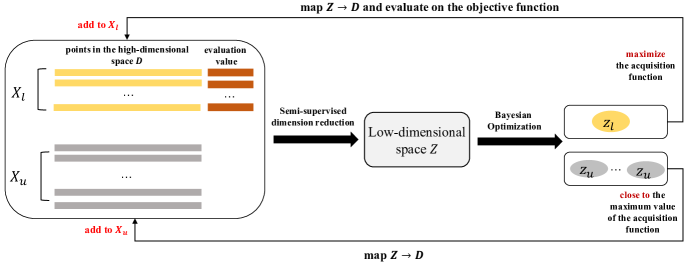
Figure 1: An overview of SILBO.

As shown in Figure 1, given the labeled points $X_{l}$ and unlabeled points $X_{u}$ where the label represents the evaluation value of the corresponding point, SILBO consists of three tightly-connected phases:

• semi-supervised embedding learning, which tries to find an effective low-dimensional space $\mathcal{Z}$ of the objective function by utilizing both $X_{l}$ and $X_{u}$;

• performing Gaussian Process regression on the learned low-dimensional embedding space and selecting candidate points according to the acquisition function of BO;

• evaluating points by the objective function $f$, then updating the Gaussian Process surrogate model and the projection matrix $B$.

Input: Objective function $f$, acquisition function $\alpha$, high dimension $d$, effective dimension $r$

Output: The optimum $x^{*}$

1 Initialize samples $X_{u}^{0},X_{l}^{0}$ with size $n_{u}$ and $n_{l}$;

2 Construct $B_{0}$ with Algorithm 2;

3 Let $D_{0}=\{B_{0}X^{0}_{l},f(X^{0}_{l})\}$;

4 Construct Gaussian Process regression model based on $D_{0}$;

5 $Z_{l}^{0}=\varnothing$,$Y_{0}=\varnothing$;

6 for $t=1$ to $N$ do

7       $Z_{u}^{t}=\varnothing$;

8       Generate random point set $C$ from the low-dimensional space;

9       $z_{l}=\arg\max_{z\in C}\alpha(z)$;

10       $Z_{l}^{t}=Z_{l}^{t-1}\cup z_{l}$;

11       $C=C-z_{l}$;

12       for $n=1$ to $n_{u}$ do

13             $z_{u}$ = $\arg\max_{z\in C}\alpha(z)$;

14             $Z_{u}^{t}\cup z_{u}$;

15             $C=C-z_{u}$;

16       end for

17      Construct $X_{l}^{t}$,$X_{u}^{t}$,$D_{t}$ based on $Z_{l}^{t}$,$Z_{u}^{t}$;

18       Update Gaussian process regression model based on $D_{t}$;

19       Update $B_{t}$ with Algorithm 2 based on $X_{u}^{t}$ , $X_{l}^{t}$ and $Y_{t}$;

20      

21 end for

Algorithm 1 SILBO

These phases are also summarized in Algorithm 1. The first step is to construct the projection matrix $B$ and find an effective low-dimensional space that can keep the information of the original space as much as possible. Both $X_{l}$ and $X_{u}$ are selected according to the acquisition function of BO. $X_{l}$ is the labeled points that have been evaluated on the objective function. $X_{u}$ is the unlabeled points whose evaluation values are unknown.

The second step is to find the possible low-dimensional optimum $\bm{z}_{l}\in\mathcal{Z}$ which maximizes the acquisition function $\alpha$ and select several promising unlabeled points $\bm{z}_{u}\in\mathcal{Z}$ that can be used to update $B$ in the next iteration. Then, $\bm{z}_{l}$ and $\bm{z}_{u}$ are mapped back to the high-dimensional space $\mathcal{D}$ through a specific mapping $h:\mathcal{Z}\rightarrow\mathcal{D}$ to get $\bm{x}_{l}$ and $\bm{x}_{u}$.

Finally, we compute $y$ by evaluating the objective function $f$ on $x_{l}$ and update the GP model by $(z_{l},y)$. The $x_{l}$ and $x_{u}$ will be added to $X_{l}$ and $X_{u}$ respectively for updating the embedding in the next iteration.

The low-dimensional embedding is learned through SIR combined with the semi-supervised technique. The between-slice scatter matrix $\Sigma_{\eta}$ and total within-slice scatter matrix $\Sigma_{x}$ are constructed by utilizing the local information as well as the unlabeled points. Then, $B$ is obtained through solving the generalized eigenvalue problem. Based on the randomized SVD method, Algorithm 2 is proposed to speed up the solution to this problem. Moreover, we carefully analyze the mapping $h$ between the low-dimensional space and the high-dimensional space and further propose two strategies for the scenarios with different evaluation costs.

4.2 Semi-supervised Dimension Reduction

The assumption is that there is a low-dimensional space that preserves the information of the objective function $f(\bm{x})$ defined in the high-dimensional space. In other words, the dimensionality of $\mathcal{D}$ can be reduced without losing the essential information to predict response values $Y$. If there are enough evaluated points for the initialization of Bayesian optimization, we may be able to explore the intrinsic structure of $f(\bm{x})$ through these points. However, for optimization problems with high computational cost, only a few evaluated points are available. Thus, it is difficult to learn proper embedding only through them. In such a case, reasonable and effective use of unevaluated points acquired from the acquisition function of BO will be helpful for embedding learning.

Although SDA provides an effective strategy to incorporate the unlabeled data, it is only suitable for classification problems. Therefore, we need to extend it to the scenarios where the response value is continuous. In fact, SIR is equivalent to LDA, and SDA is an extension of LDA as a generalized eigenvalue problem (Wu et al., 2010). Thus, SDA can be applied to regression setting by taking advantage of the discreteness brought by the slicing technique in SIR. We call such extension semi-SIR. Next, we introduce how to construct semi-SIR to learn a low-dimensional embedding.

First, the evaluated points are sorted and cut into $H$ slices according to their response values. Then, similar to SDA (Cai et al., 2007), our problem can be reformulated as follows. Given labeled points $X_{l}\in\mathbb{R}^{n_{l}\times d}$ and unlabeled points $X_{u}\in\mathbb{R}^{n_{u}\times d}$, $n_{l}$ and $n_{u}$ denote the number of the labeled and unlabeled points respectively, we aim to find the embedding matrix $B$ through solving:

$$X^{\top}WX\beta=\lambda X^{\top}(\hat{I}+\alpha L)X\beta$$ (11)

where $X\in\mathbb{R}^{n\times d}$ denotes a centered data matrix whose rows represent $n$ samples in $\mathbb{R}^{d}$, $n=n_{u}+n_{l}$. $W$ is a $n\times n$ weight matrix. $\hat{I}$ can be expressed as:

$$\hat{I}=\begin{bmatrix}I&0\\ 0&0\end{bmatrix}$$ (12)

where $I$ is a $n_{l}\times n_{l}$ identity matrix.

Note that the between-slice scatter matrix $X^{\top}WX$ can be written in an elegant linear algebraic formulation.

$$X^{\top}WX=X^{\top}\Omega\Omega^{\top}X=X^{\top}\begin{bmatrix}\Omega_{l}\Omega^{\top}_{l}&0\\ 0&0\end{bmatrix}X$$ (13)

where $\Omega_{l}\in\mathbb{R}^{n_{l}\times H}$ denotes the rescaled slice membership matrix for those evaluated samples with $\Omega_{l_{ij}}=1/\sqrt{n_{j}}$ if the $i$-th sample of $X_{l}$ is a member of the $j$-th slice. Otherwise, $\Omega_{l_{ij}}=0$. $n_{j}$ denotes the number of the samples in the $j$-th slice.

For the labeled points in the same slice, their response values are very close, but this closeness may not be retained in $\mathcal{D}$. There could be a small number of points that are far away from others in each slice. Although these outliers may indicate that there exist other areas with large response values of the objective function, they are likely to interfere with the embedding we have learned. Thus, to reveal the main information of the objective function as much as possible, we employ the localization technique. By strengthening the local information of each slice, the degeneracy issue in the original SIR can be mitigated (Wu et al., 2010). Next, we illustrate how to construct $W$ in Equation 13 with the local information.

We note that $\Omega_{l}$ in Equation 13 is a block matrix, and each block corresponds to a slice.

$$\Omega_{l}=\begin{pmatrix}\Omega_{l}^{1}&&\\ &\ddots&\\ &&\Omega_{l}^{H}\end{pmatrix}$$ (14)

For the original between-slice scatter $X^{\top}WX$, $\Omega_{l}$ can only indicate whether a sample point belongs to a slice. Here, we will strengthen the localization information by introducing a localized weight. For those evaluated samples, we let $\Omega^{h}_{ij}=1/k_{h}$ if the $i$-th sample belongs to the $k$-nearest neighbors of the $j$-th sample ($j$ can equal to $i$) in the $h$-th slice. Otherwise, $\Omega^{h}_{ij}=0$. $H$ denotes the number of slices, $k$ is a parameter for $k$NN, and $k_{h}$ is the number of neighbor pairs in the $h$-th slice.

In summary, we aim to estimate the intrinsic structure of the objective function and find an effective subspace that reflects the large response value. Then, we are in a better position to identify the possible global optimum. Therefore, in combination with Bayesian optimization whose acquisition function will provide us candidate points with potentially large response values, semi-supervised dimension reduction can alleviate overfitting caused by the small size of labeled points. Thus, by utilizing both the labeled and unlabeled points, we can learn an $r$-dimensional space that preserves the intrinsic structure of the objective function better.

4.3 Randomized Semi-supervised Dimension reduction

In the high-dimensional scenario, learning a low-dimensional embedding space still requires a lot of time. The main bottleneck lies in the solution of generalized eigenvalue problem in Equation 11 and the computation of the neighbor information in each slice. The major computation cost of the traditional method such as the two-stage SVD algorithm is the decomposition of the large-scale matrix. Fortunately, the randomized SVD (R-SVD) technique (Halko et al., 2011) shed a light on this problem.

The contribution of R-SVD here is that when the effective dimension $r\ll n<d$, using randomized SVD to approximate a $n\times d$ matrix only requires $O(ndr)$, rather than $O(n^{2}d)$. Moreover, the empirical results find that when solving the generalized eigenvalue problem, the performance of the randomized algorithm is superior to that of the traditional deterministic method in the high-dimensional case (Georgiev and Mukherjee, 2012). Thus, we first replace the two-stage SVD with R-SVD to accelerate the solution of Equation 11.

We note that the decomposition overhead of the $X^{T}\Omega\in\mathbb{R}^{d\times n}$ in Equation 11 is huge when $d$ is large. Thus, we decompose $X^{\top}\Omega=U_{1}S_{1}V_{1}^{\top}$ using the R-SVD algorithm. Then, the between-slice scatter matrix can be expressed as:

$$X^{\top}\Omega\Omega^{\top}X=U_{1}S_{1}^{2}U_{1}^{\top}$$ (15)

Similarly, due to the symmetry of matrix $\hat{I}+\alpha L$, the right hand side of Equation 11 can be decomposed as:

$$X^{\top}(\hat{I}+\alpha L)X=X^{\top}MM^{\top}X$$ (16)

where $M$ can be constructed through Cholesky decomposition. Thus, the generalized eigenvalue problem in Equation 11 can be reformulated as:

$$\frac{1}{\lambda}e=S_{1}^{-1}U_{1}^{\top}X^{\top}MM^{\top}XU_{1}S_{1}^{-1}e$$ (17)

where $e=S_{1}U_{1}^{T}\beta$.

Next, if we let $A=S_{1}^{-1}U_{1}^{\top}X^{\top}M$, then we can see that this is a traditional eigenvalue problem. $A$ is an $r\times n$ matrix, $r$ is small enough and thus we can decompose it through original SVD naturally: $A=U_{2}S_{2}V_{2}^{\top}$. Finally, the embedding matrix can be computed as:

$$B=(U_{1}S_{1}^{-1}e_{1},\cdots,U_{1}S_{1}^{-1}e_{r})=U_{1}S_{1}^{-1}U_{2}$$ (18)

The original time complexity of the construction of $X^{T}\Omega\in\mathbb{R}^{d\times n}$ and $X^{T}M\in\mathbb{R}^{d\times n}$ is $O(d^{2}nn_{h})$ and $O(d^{2}nk)$ respectively, including the computation of the exact $k$NN for each point, where $n_{h}$ is the number of samples in each slice. In addition, the time complexity of decomposition of $X^{T}\Omega$ is $O(n^{2}d)$ and the time complexity of construction and computation of Equation 17 is $O(ndr)$. Therefore, the overall time complexity is $O(d^{2}n\max(n_{h},k)+n^{2}d+ndr)$, which is prohibitive in the high-dimensional case.

To alleviate the expensive overhead in high-dimensional case, we use the fast $k$NN (Achlioptas, 2003; Ailon and Chazelle, 2009) to compute the neighbor information, we find that constructing $X^{T}\Omega$ and $X^{T}M$ only requires $O(tdnn_{h})$ and $O(tdnk)$ respectively. Moreover, using R-SVD to factorize the matrix $X^{T}\Omega$ only requires $O(ndr)$. Therefore, The overall time complexity reduces to $O(tdn\max(n_{h},k)+ndr)$. $t$ denotes a fixed parameter about the logarithm of $n$.

Algorithm 2 summarizes the above steps.

Input: $X_{l}\in\mathbb{R}^{n_{l}\times d}$, $X_{u}\in\mathbb{R}^{n_{u}\times d}$, number of slice $H$; number of nearest neighbor $k$, effective dimension $r$

Output: $B\in\mathbb{R}^{d\times r}$

1

2compute $X^{\top}\Omega$, $X^{\top}M$ from Equation 13 and Equation 16;

3 estimate $[U_{1},S_{1},V_{1}]$ = Randomized SVD($X^{\top}\Omega$,$r$);

4 $A=S_{1}^{-1}U_{1}X^{\top}M$;

5 factorize $[U_{2},S_{2},V_{2}]$= SVD($A$);

6 compute $B$ from Equation 18

Algorithm 2 Randomized semi-supervised dimension reduction

4.4 Mapping From Low to High

After semi-supervised dimensional reduction, we perform Bayesian optimization with GP on the low-dimensional space $\mathcal{Z}$. But we need to further consider three issues. The first is how to select the search domain $S$ in the low-dimensional embedding space. The second is how to specify a mapping $h$ associate with $B$ to map the point $\bm{z}$ from the embedding space $\mathcal{Z}$ to the high-dimensional space $\mathcal{D}$ where the response value $y$ should be evaluated. The third is how to maintain consistency of the Gaussian process regression model after updating $B$. Only by addressing these issues, the low-dimensional Bayesian optimization can be updated by the data pair $(\bm{z},y)$.

Before elaborating the selection of $S$ in the first issue, we introduce the definition of zonotope, which is a convex symmetric polytope.

Definition 1

Zonotope (Le et al., 2013) Given a linear mapping $H\in\mathbb{R}^{r\times d}$ and vector $\bm{p}\in\mathbb{R}^{r}$, an r-zonotope is defined as

$$Z=\{\bm{z}\in\mathbb{R}^{r}:\bm{z}=\bm{p}+H\bm{x};\bm{x}\in[-1,1]^{d}\}$$

where $\bm{p}$ is the center vector of the zonotope.

Without loss of generality, let $\bm{p}=\bm{0}$, we note that $H$ is exactly $B$ computed by Equation 18. Thus, the zonotope $Z_{B}$ associate with $B$ is the low-dimensional space where Bayesian optimization is performed. Then, we introduce the smallest box containing the zonotope.

Lemma 2

Given zonotope $Z=\{\bm{z}\in\mathbb{R}^{r}:\bm{z}=\bm{p}+H\bm{x};\bm{x}\in[-1,1]^{d}\}$, $\bm{p}=\bm{0}$, the smallest box containing this zonotope can be computed as

$$S=\left[-\sum^{d}_{j=1}\left|H_{1j}\right|,\sum^{d}_{j=1}\left|H_{1j}\right|\right]\times\cdots\times\left[-\sum^{d}_{j=1}\left|H_{rj}\right|,\sum^{d}_{j=1}\left|H_{rj}\right|\right]$$

Although the boundary of zonotope is difficult to solve, we use the box $S$ as an alternative (Binois et al., 2019).

Next, we focus on the second and third issues. As mentioned before, a mapping $h$ should connect the high-dimensional space and the low-dimensional space. As a result, for any point in the low-dimensional space, a corresponding point can be found in the high-dimensional space. In this way, the low-dimensional point $\bm{z}$ and the response value $y$ of the corresponding high-dimensional point $\bm{x}$ can be used as the training set to build a Gaussian process regression model. Figure 2 shows the relationship between them. We note that the reproduction of the correlation between $\bm{z}$ and $y$ is the goal of the low-dimensional Gaussian process regression model, and the two are closely connected through $\bm{x}$. Thus a reasonable choice of $h$ plays a great influence on such a middle layer. Meanwhile, due to the iterative nature of SILBO, the mapping $h$ will change after updating $B$, which directly makes the correlation between $\bm{z}$ and $y$ inconsistent before and after the update. Therefore, we need to develop a strategy to maintain consistency. Next, we introduce two different strategies to address these two issues.

Input: Labeled low-dimensional points $Z_{l}^{t}$, unlabeled low-dimensional points $Z_{u}^{t}$

Output: Labeled high-dimensional points $X_{l}^{t}$, unlabeled high-dimensional points $X_{u}^{t}$, the training set $D_{t}$

1

2$X_{l}^{t}=B_{t}^{\dagger}Z_{l}^{t}$;

3 $X_{u}^{t}=B_{t}^{\dagger}Z_{u}^{t}$;

4 $Y_{t}=f(X^{t}_{l})$, $D_{t}=(Z_{l}^{t},Y_{t})$;

5

Algorithm 3 The $bottom$-$up$ strategy

As shown in Algorithm 3, we can naturally get the response value $y$ by evaluating the point $\bm{x}=B^{\dagger}\bm{z}$ after finding the candidate point $\bm{z}\in S$ through BO. When the projection matrix $B$ changed, we fix $z$ at the bottom of the hierarchy in Figure 2(a) and then update $y$ at the top to maintain consistency ($bottom$-$up$ for short).

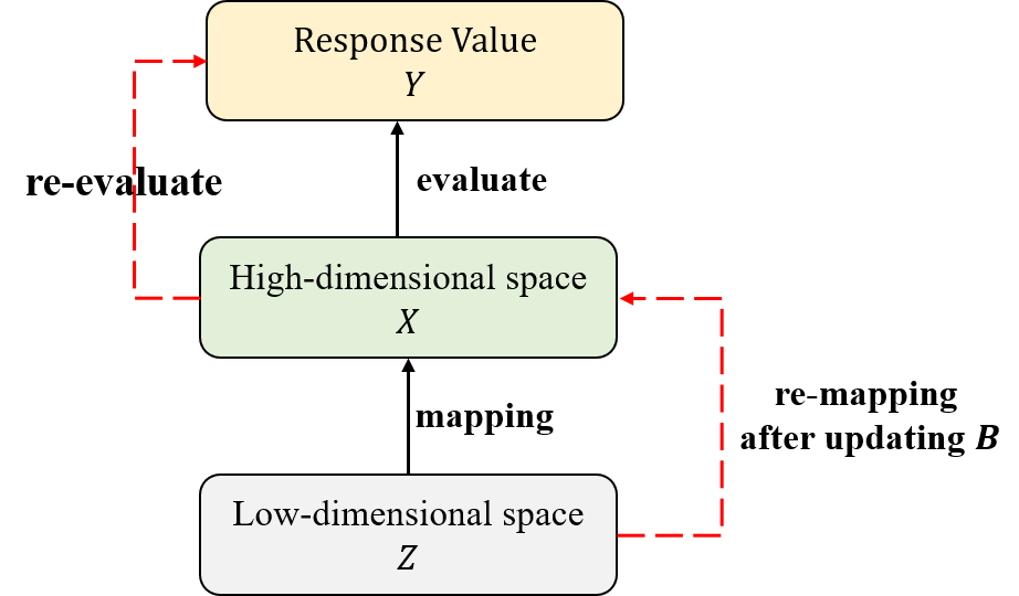
(a) Bottom-up strategy

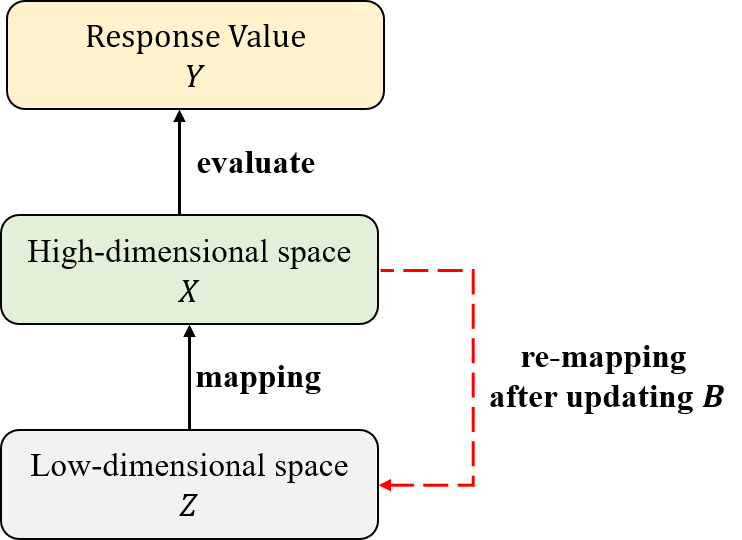
(b) Top-down strategy

Figure 2: The relationship between response value $y$, high-dimensional point $x$, and low-dimensional point $z$. The solid line shows the process of mapping and evaluation with different strategies. The left hierarchy denotes the $bottom$-$up$ strategy. The dash line shows the process of re-mapping and re-evaluation. $z$ at the bottom is fixed after updating $B$. Then, re-map $z$ to find and re-evaluate the corresponding $x$. The right hierarchy shows the $top$-$down$ strategy. The dash line shows the re-mapping process. $x$ and $y$ at the top are fixed after updating $B$. Then, $x$ is re-mapped to find the corresponding $z$ and a new Gaussian Process regression model will be constructed.

Since we use $B^{\dagger}$ to connect the points between the low-dimensional space $\mathcal{Z}$ and the high-dimensional space $\mathcal{D}$, the actual evaluation space $\phi$ is only a part of $\mathcal{D}$ (i.e., $\phi\subset\mathcal{D}$) when $B$ is fixed. While a great probability of containing the optimum in $\phi$ has been proved (Wang et al., 2013), one of the preconditions is that there is no limitation to the high-dimensional space of the objective function. In practice, the restriction often exists (e.g., $[-1,1]^{d}$), making the high probability no longer guaranteed. In contrast, due to the iterative nature of the effective low-dimensional space learning mechanism in SILBO (Algorithm 1), we can alleviate this problem. Specifically, more and more $\phi$ associate with $B$ will be learned, which gradually reveal the location of the optimum.

However, the $bottom$-$up$ strategy may bring more evaluation overhead. When we get the training set $D_{t}=\{\bm{z}_{i},y_{i}\}_{i=1}^{T}$ for BO through $T$ iterations in Algorithm 1, we update $B$ to $B_{new}$ and get $\bm{z}_{T+1}$ through the acquisition function $\alpha$. Due to the updating of $B$, the mapping relationship between the high-dimensional and low-dimensional spaces has changed. As shown in Figure 2(a), we need to find the corresponding $\bm{x}$ again for $\bm{z}$ in the training set and then evaluate $\bm{x}$ to maintain consistency. When the evaluation of the objective function is expensive, the computational cost is huge.

To eliminate the re-evaluation overhead, we propose a new strategy. Specifically, we first obtain $\bm{z}$ in the low-dimensional space through the acquisition function $\alpha$, and then solve the following equation to find the corresponding $\bm{x}$.

$$\mathop{\arg\min}\limits_{\bm{x}}||B\bm{x}-\bm{z}||^{2}$$ (19)

When the projection matrix $B$ is changed, we fix $\bm{x}$ and $y$ at the top of the hierarchy in Figure 2 and then update $\bm{z}$ in the bottom to maintain consistency ($top$-$down$ for short).

Input: Labeled low-dimensional points $Z_{l}^{t}$, unlabeled low-dimensional points $Z_{u}^{t}$, labeled high-dimensional points $X_{l}^{t-1}$, the training set $D_{t-1}$

Output: labeled high-dimensional points $X_{l}^{t}$, unlabeled high-dimensional points $X_{u}^{t}$, the training set $D_{t}$

1

2Get the last point $z_{l}$ from $Z_{l}^{t}$;

3 Compute $x_{l}$,$X_{u}^{t}$ from Equation 19 using $z_{l}$,$Z_{u}^{t}$;

4 $X^{t}_{l}=X_{l}^{t-1}\cup x_{l}$;

5 $y=f(x_{l})$, $D_{t}=D_{t-1}\cup(\bm{z}_{l},y)$;

6

Algorithm 4 The $top$-$down$ strategy

Different from the $bottom$-$up$ strategy, the $top$-$down$ strategy shown in Figure 2(b) updates $\bm{z}$ directly, which enables us to reconstruct a new BO model efficiently only by replacing the training set with $\{B_{new}\bm{x}_{i},y_{i}\}_{i=1}^{T}$ after updating $B$, instead of relocating $\bm{x}$ and re-evaluating them. The $top$-$down$ strategy can be found in Algorithm 4. Next, we analyze the rationality of this strategy theoretically.

Theorem 3

Given a matrix $B\in\mathbb{R}^{r\times d}$ with orthogonal rows and its corresponding zonotope $Z_{B}$. Given $\bm{z}\in Z_{B}$, for any $\bm{x}_{1},\bm{x}_{2}\in U_{B}=\{\bm{x}|\bm{x}=B^{\top}\bm{z}+y,\bm{x}\in\mathbb{R}^{d},y\in\text{N}(B)\}$, $B\bm{x}_{1}=B\bm{x}_{2}=\bm{z}$.

Proof  Let $\bm{x}=\bm{x}_{V}+\bm{x}_{V}^{\bot}\in\mathbb{R}^{d}$ be the orthogonal decomposition with respect to $V$ = Row($B$), then $\bm{x}_{V}\in V$. Let $\bm{z}\in Z_{B}$ with $B^{\top}\bm{z}=\bm{x}_{V}$. Due to the orthogonal decompostion, we have $\bm{x}-\bm{x}_{V}=\bm{x}-B^{\top}\bm{z}$ lies in $V^{\bot}=\text{N}(B)$. For any $\bm{x}_{1},\bm{x}_{2}\in U_{B}$, we have $\bm{x}_{1}-\bm{x}_{V}=\bm{x}_{1}-B^{\top}\bm{z}$ and $\bm{x}_{2}-\bm{x}_{V}=\bm{x}_{2}-B^{\top}\bm{z}$, then $B(\bm{x}_{1}-B^{\top}\bm{z})=B(\bm{x}_{2}-B^{\top}\bm{z})=0$. Thus, $B\bm{x}_{1}=B\bm{x}_{2}=BB^{\top}\bm{z}=\bm{z}$.  

According to Theorem 3, if we assume that $B$ has orthogonal rows, it is clear that given $B$ and $\bm{z}$, any point $\bm{x}\in U_{B}$ will be the solution to Equation 19. However, our purpose is not $\bm{x}$ itself, but $y=f(\bm{x})$, because $(\bm{z},y)$ is the data pair used to update BO. Fortunately, if we use SILBO to learn an ideal effective low-dimensional subspace $B^{*}$, then for any $\bm{x}_{1},\bm{x}_{2}$ in the solution set $U_{B^{*}}$, $f(\bm{x}_{1})=f(B^{*\top}\bm{z}+y_{1})=f(B^{*\top}\bm{z})$, $f(\bm{x}_{2})=f(B^{*\top}\bm{z}+y_{2})=f(B^{*\top}\bm{z})$ (i.e., $f(\bm{x}_{1})=f(\bm{x}_{2})$). Thus, in each iteration $T$, we can obtain the unique data pair $(\bm{z}_{T},y_{T})$ under $B^{*}$ to update the low-dimensional Bayesian optimization model. Therefore, the diversity of solutions in the set $U_{B}$ does not affect the construction of BO and we can explore in the original space $\mathcal{D}$ which liberates the shackles of $\phi$.

In summary, both the two strategies aim to generate a consistent training set for the subsequent GP construction when updating $B$. To maintain such consistency, the $bottom$-$up$ strategy acquires more observations $y$ from the objective function according to $\bm{z}$ in the training set while the $top$-$down$ strategy directly changes $\bm{z}$ according to $y$. Note that the more response values, the more information about the objective function we can get. Thus, the $bottom$-$up$ strategy can obtain more clues about the global optimum than the $top$-$down$ strategy.

5 Numerical Results

In this section, we evaluated our proposed algorithm SILBO on a set of high-dimensional benchmarks. First, we compared SILBO with other state-of-the-art algorithms on synthetic function and neural network hyperparameter optimization tasks. Second, we demonstrated the effectiveness of semi-supervised embedding learning and iterative learning. Finally, we evaluated and analyzed the scalability of SILBO.

5.1 Experiment Setting

For comparison, we also evaluated other state-of-the-art algorithms: REMBO (Wang et al., 2013), which performs BO on a random generated linear embedding space, REMBO-$K_{X}$, which computes the kernel using the distance in the high-dimensional space, REMBO-$K_{\psi}$ (Binois et al., 2015), which uses a warping kernel and finds the evaluation point through sophisticated mapping, and HeSBO (Nayebi et al., 2019), which uses the count-sketch technique to generate subspace and compute the projection matrix. Additional methods include ADD-BO (Kandasamy et al., 2015), which assumes that the objective function has an additive structure, and recently-proposed SIR-BO (Zhang et al., 2019), which uses SIR to learn a low-dimensional space purely. SILBO-BU and SILBO-TD represent the proposed SILBO algorithm that employs the $bottom$-$up$ and $top$-$down$ mapping strategies respectively.

We employed the package GPy as the Gaussian Process framework and selected the Matérn kernel for the GP model. We adopted the package ristretto to perform the R-SVD. We employed CMA-ES (Hansen, 2016) to compute Equation 19 for SILBO-TD. The embedding matrix $B$ is updated every 20 iterations. The size of the unlabeled points is set to 50 in each iteration. The number of neighbors $k$ is set to $7$ and the number of unlabeled points is set to $50$ for semi-supervised dimension reduction. To obtain error bars, we performed 100 independent runs for each algorithm on synthetic functions and 5 runs for the neural network hyperparameter search. We plotted the mean value along with one standard deviation. For ADD-BO, we used the authors’ implementation through $MATLAB$, so we did not compare its scalability since other algorithms were implemented in $Python$. Also, we evaluated SILBO using two acquisition functions: UCB and EI. The number of initial random points defaults to 50 and the response values of initial points are not considered when observing the experimental performance except in Section 5.5, which uses different number of initial points, so the response values of these points are shown in the performance curve.

5.2 Performance on Synthetic Functions

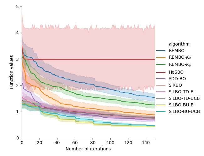
(a) 100d Branin

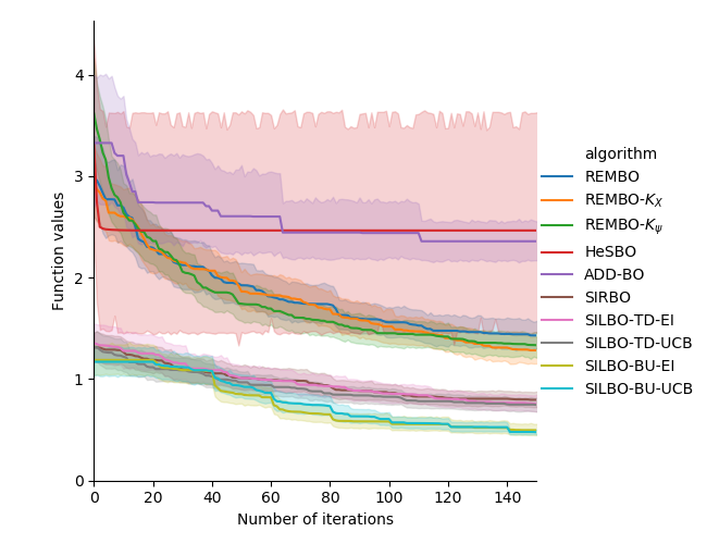
(b) 1000d Branin

Figure 3: Performance on Branin under dimension 100(a) and dimension 1000(b) with embedding dimension $r$ = 2. We plotted mean and one standard deviation across 100 independent runs.

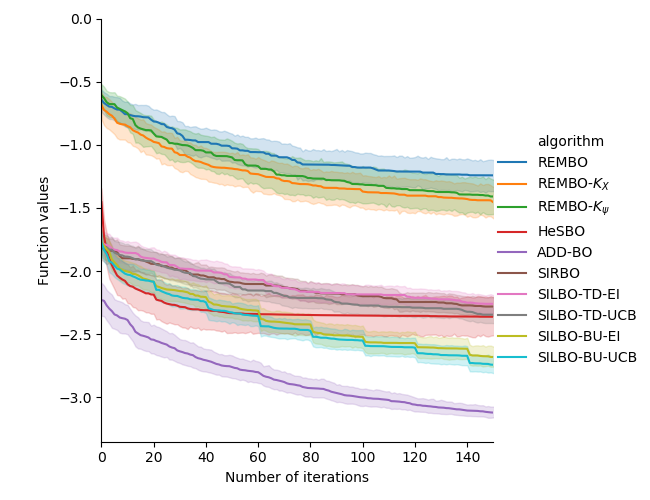
(a) 100d hartmann6

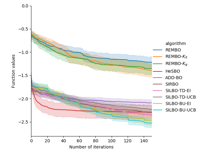
(b) 1000d hartmann6

Figure 4: Performance on Hartmann6 under dimension 100(a) and dimension 1000(b) with embedding dimension $r$ = 6. We plotted mean and one standard deviation across 100 independent runs.

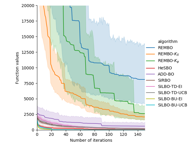
(a) 100d Colville

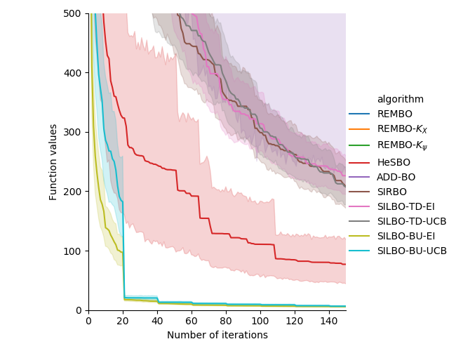
(b) 100d Colville (enlarged)

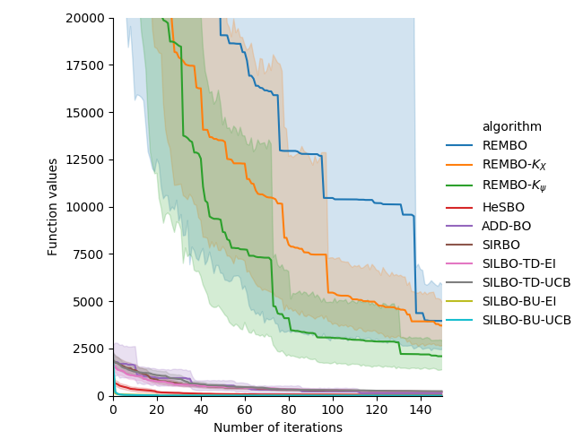
(c) 1000d Colville

(d) 1000d Colville (enlarged)

Figure 5: Performance on Colville under dimension 100(a)(b) and dimension 1000(c)(d) with embedding dimension $r$ = 4. To see performance discrepancy clearly among different algorithms, we enlarged (a)(c) to get (b)(d) respectively. We plotted mean and one standard deviation across 100 independent runs.

Similar to (Nayebi et al., 2019), these algorithms were under comparison upon the following widely-used test functions: (1) Branin (2) Hartmann-6 (3) Colville. The active dimensions for Branin, Hartmann-6, Colville are 2, 6, and 4 respectively. We studied the cases with different input dimensions $d\in\{100,1000\}$. The experimental results are shown in Figure 3-5. The proposed SILBO-BU, outperforms all benchmarks especially in high dimensions ($d=1000$). SILBO-TD is also very competitive, surpassing most traditional algorithms. In addition, the experimental results under different acquisition functions are similar. ADD-BO performs excellently in Hartmann-6 due to the additive structure of the objective function itself, but it performs poorly in the 1000-dimension case (Figure 4(b)) and in functions without the additive structure. HeSBO performs well in Colville and Hartmann-6, but poorly in Branin. Moreover, we can find that HeSBO does not converge in most cases. The performance of SIRBO is similar to our proposed SILBO-TD since it also tries to learn an embedding space actively. In summary, the proposed method SILBO-BU nearly beats all baselines due to effective semi-supervised dimension reduction and iterative embedding learning.

5.3 Hyperparameter Optimization on Neural Network

Following (Oh et al., 2018), we also evaluated SILBO in a hyperparameter optimization task for a neural network on the MNIST dataset. Specifically, the neural network is a multi-Layer perceptron (MLP) with one hidden layer of size 50 and one output layer of size 10. These 500 initial weights were viewed as hyperparameters and were optimized using the Adam (Kingma and Ba, 2015) optimizer.

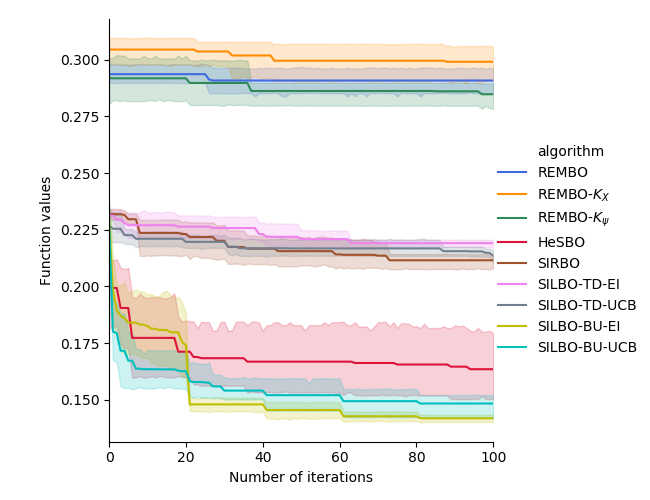
Figure 6: Performances on the MLP with embedding dimension $r$= 12. We plotted mean and one standard deviation across 5 independent runs.

Figure 6 shows that SILBO-BU converges faster than all other algorithms. The performance of SILBO-TD and SIRBO is close. These two methods perform better than other traditional methods such as REMBO and show competitive performance. Similar to the performance on synthetic functions, SILBO-BU beats all other high-dimensional BO methods and can obtain better response values in the neural network hyperparameter optimization tasks. Next, we evaluated the effectiveness of semi-supervised dimension reduction and iterative embedding learning respectively.

5.4 Effectiveness of Semi-supervised Dimension Reduction

For the function with effective dimensions, the low-dimensional subspace can reflect its intrinsic structure information. Thus, if we sample points from the function and project them into the effective subspace, the response values of these points will be dispersed along the direction of each subspace basis. Here, we compared the embedding learning performance of SILBO and SIR on Branin and Camel functions. We first evaluated 50 high-dimensional (i.e., 1000 dimensions) points to get their response values and then projected these points into the low-dimensional space generated by SILBO and SIR respectively. The goal of embedding learning is to find the e.d.r directions that preserve the information of the objective function as much as possible. Figure 7 and Figure 8 summarize the observed performance.

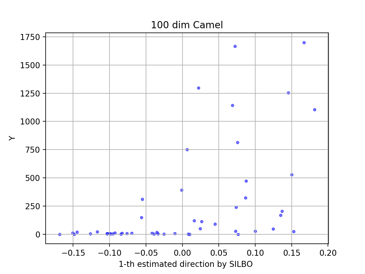
(a)

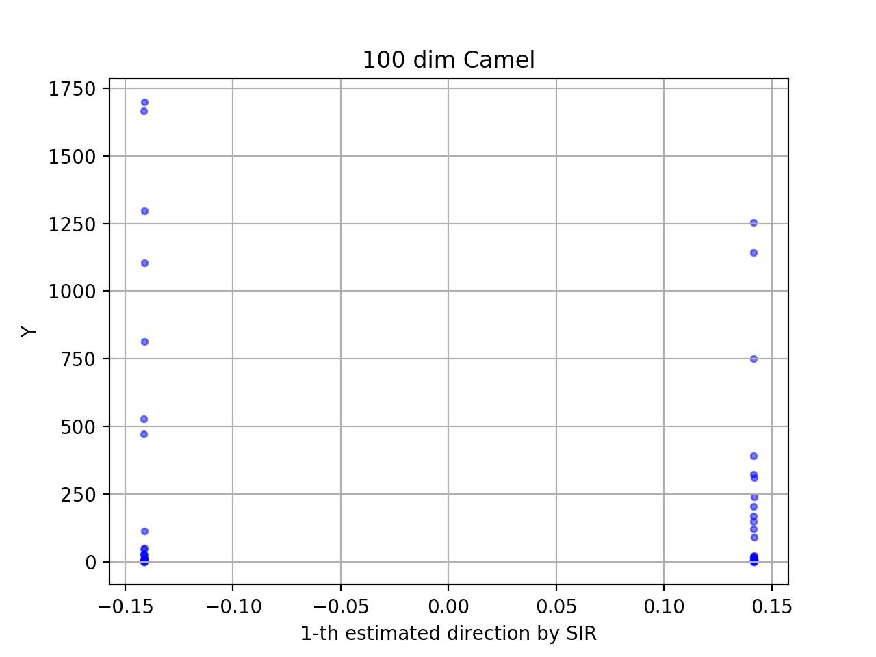
(b)

Figure 7: Point distribution in the low-dimensional space generated by SILBO and SIR respectively on Camel. The number of e.d.r directions is 1.

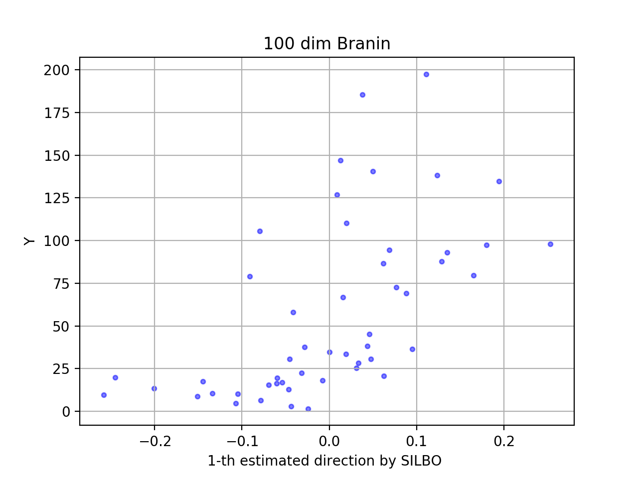
(a)

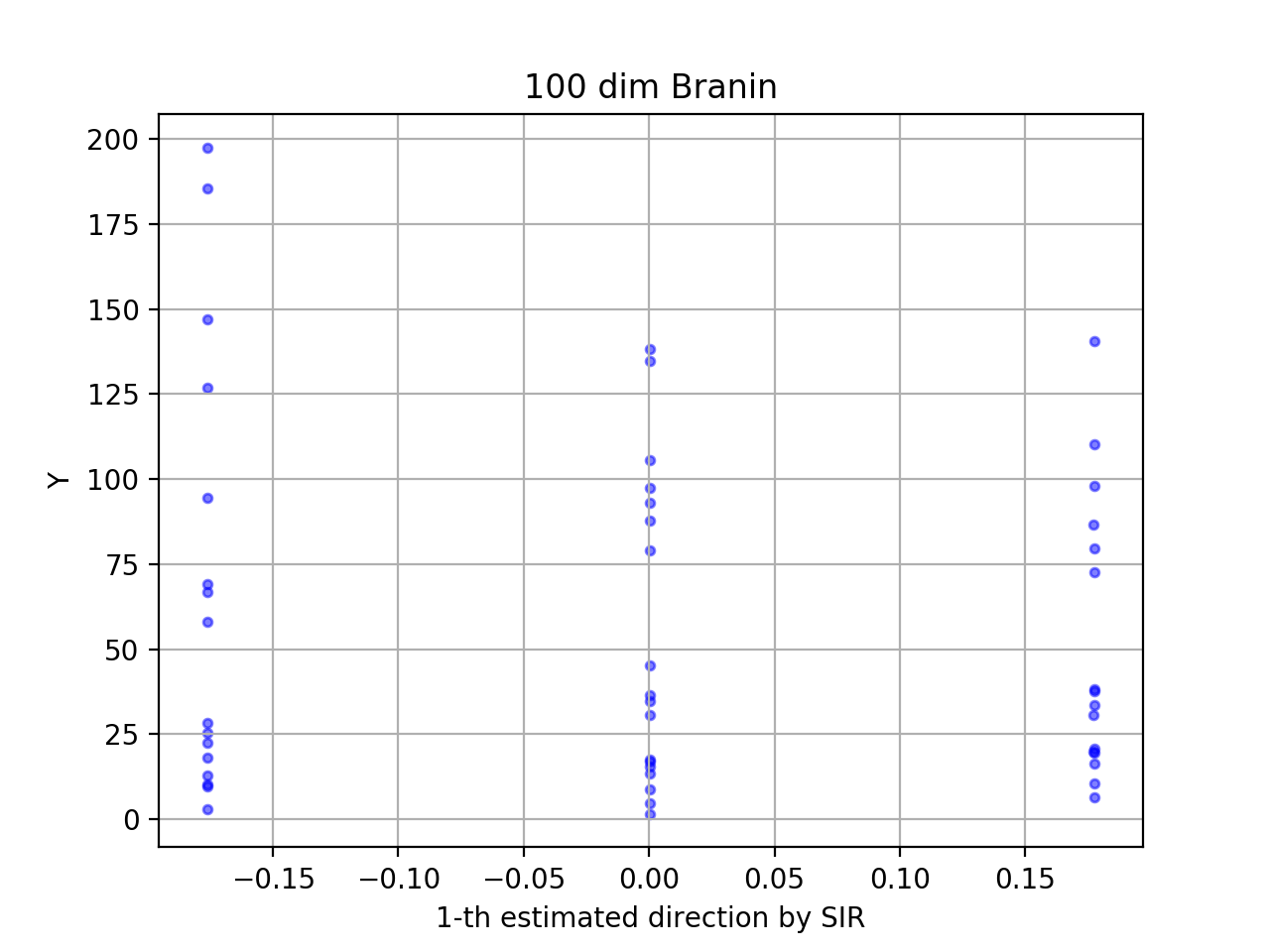
(b)

(c)

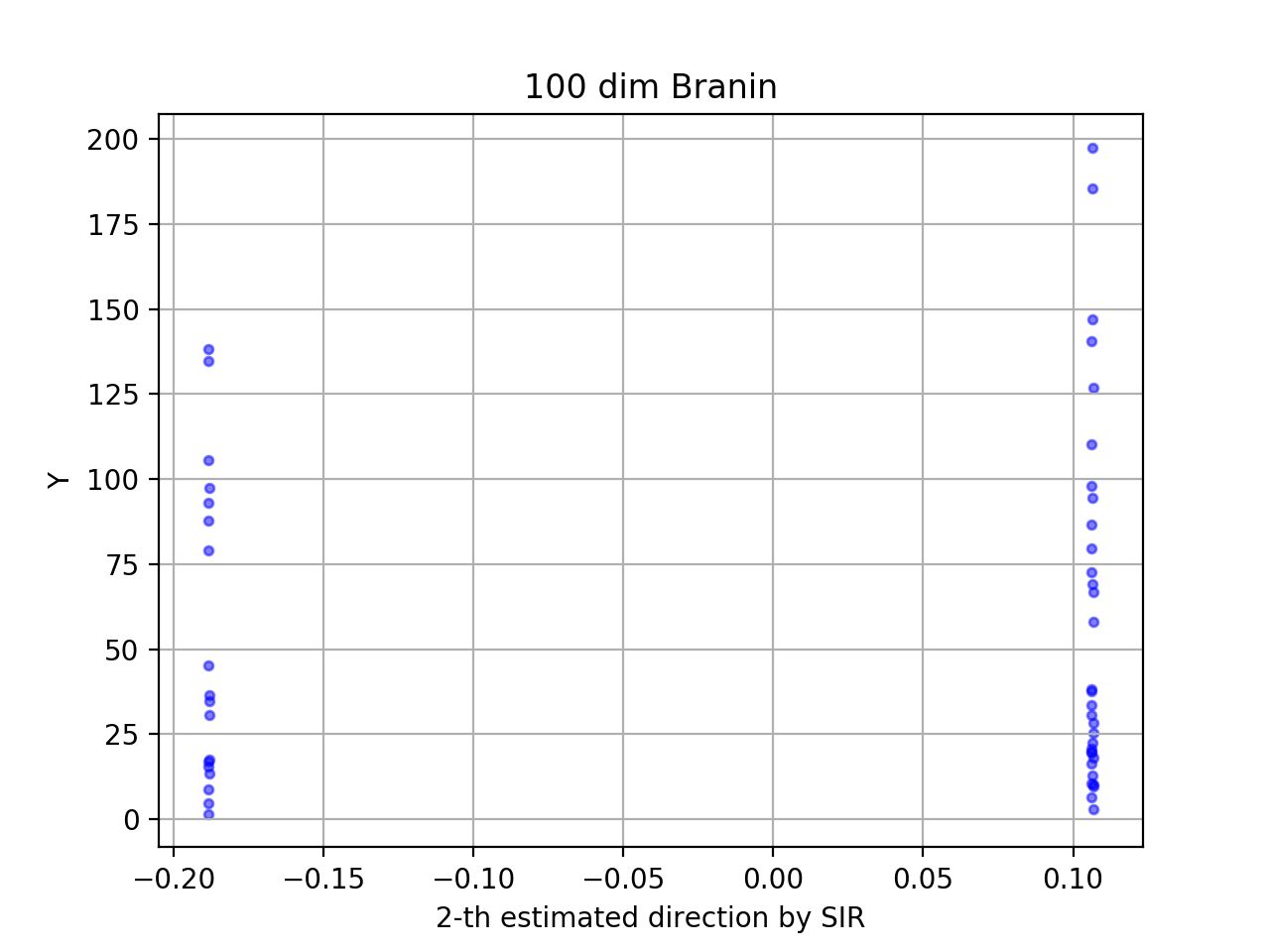
(d)

Figure 8: Point distribution in the low-dimensional space generated by SILBO and SIR respectively on Branin. The number of e.d.r directions is 2. (a)(b) plot the points projected to one estimated direction. (c)(d) plot the points projected to the other direction.

In Figure 7(b), Figure 8(b), and Figure 8(d), the information extracted by SIR stacks together. A large number of points are distributed in a very small interval, but correspond to many different response values with large variance. The consequence is that a lot of information will be lost if we train a Gaussian process regression model using these low-dimensional representations. In contrast, due to the semi-supervised dimension reduction, the information extracted by SILBO is more complete without losing the intrinsic information of the objective function.

To further demonstrate the effectiveness of semi-supervised dimension reduction, we also evaluated SILBO only using the labeled points in each iteration. We call this method SILBO-only-labeled. Figure 9 shows the comparison results between SILBO-semi and SILBO-only-labeled with the $bottom$-$up$ mapping strategy. From Figure 9, we can see that the semi-supervised dimension reduction technique can significantly improve the performance of high-dimensional Bayesian optimization.

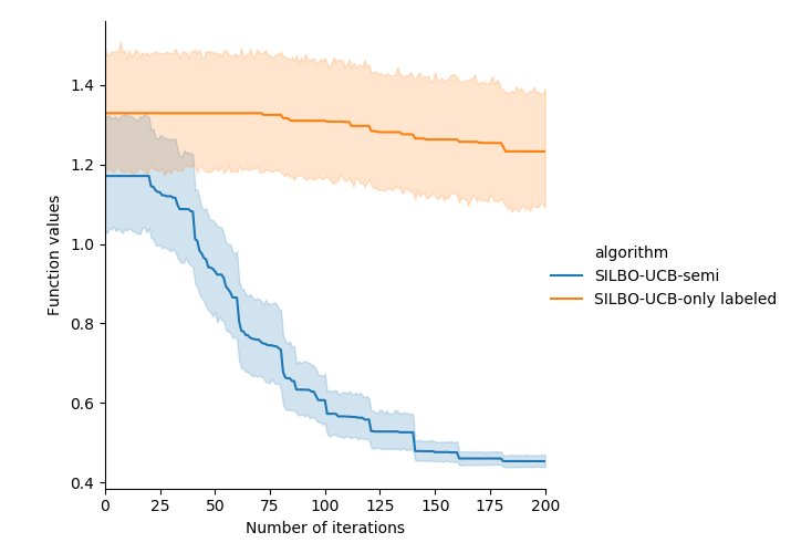
(a) 1000d Branin

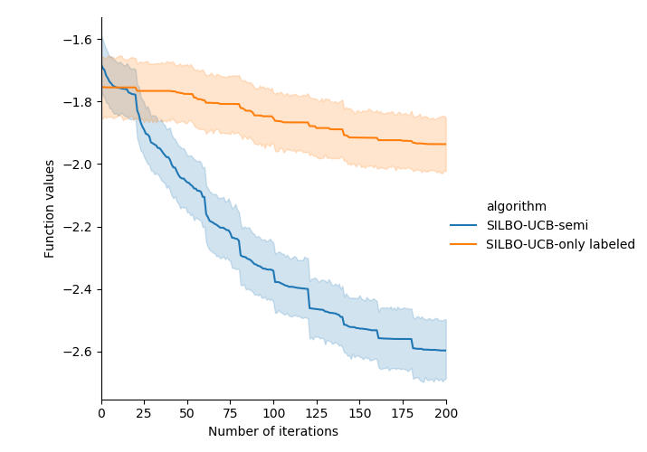
(b) 1000d Hartmann6

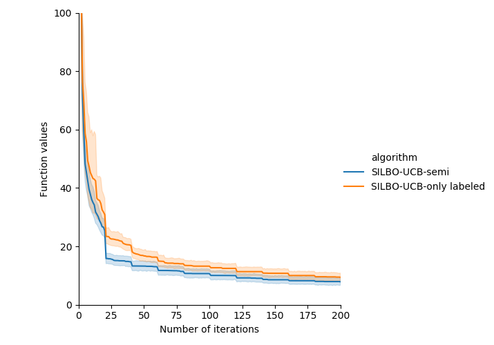
(c) 1000d Colville

Figure 9: Performance comparison between SILBO-semi and SILBO-only-labeled on three synthetic functions. All of the methods update the projection matrix every 20 iteration.

5.5 Effectiveness of Iterative Learning

In the iterative process of SILBO, the projection matrix is updated based on random initial points and the points acquired from the acquisition function. To verify the effectiveness of iterative learning, we need to show that the points acquired from the acquisition function indeed contribute to generating a better embedding. Figure 10 shows the performance comparison results with and without the iterative learning process. SILBO-only-random means that the low-dimensional embedding is learned only using the random initial points, while SILBO-random+acquisition contains the random initial points and the points from the acquisition function.

We chose 20 random initial points for SILBO-only-random and chose 10 random initial points accompanied with 10 points acquired from the acquisition function iteratively for SILBO-random+acquisition. We compared the optimization performance of the two algorithms after these 20 points. From Figure 10, we can see that SILBO-random+acquisition can find a better solution at most cases, which indicates the effectiveness of iterative learning. The main reason why SILBO-random+acquisition performs slightly worse on Branin is due to less initial points. Moreover, the performance of SILBO-random+acquisition in Figure  10 is worse than other experiments for two reasons. One is that the initial points are much less, we only use 20 initial points. The other is that the low-dimensional embedding space is only updated once.

Furthermore, we compare the optimization performance of SILBO with $bottom$-$up$ strategy under different embedding updating frequency. Figure 11 shows that the optimization performance is improved when using low updating frequency.

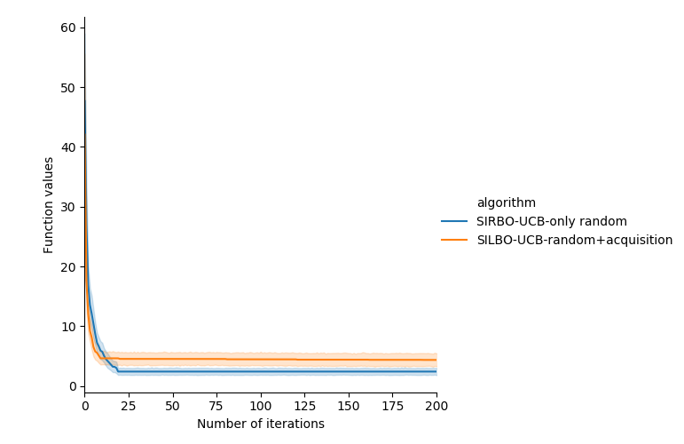
(a) 1000d Branin

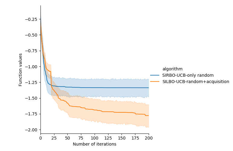
(b) 1000d Hartmann6

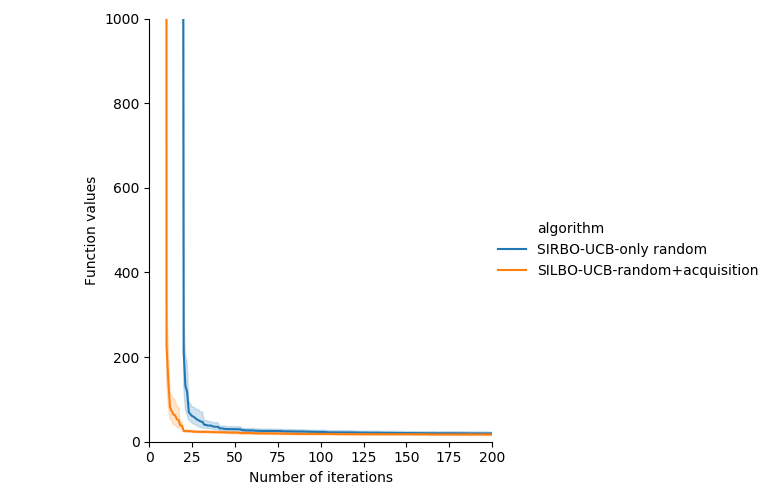
(c) 1000d Colville

Figure 10: The optimization performance of SILBO-only-random and SILBO-random+acquisition using 20 points to find the low-dimensional embedding space. The total number of points to construct the projection matrix is the same.

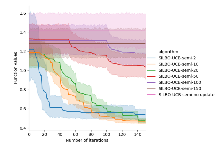
(a) 1000d Branin

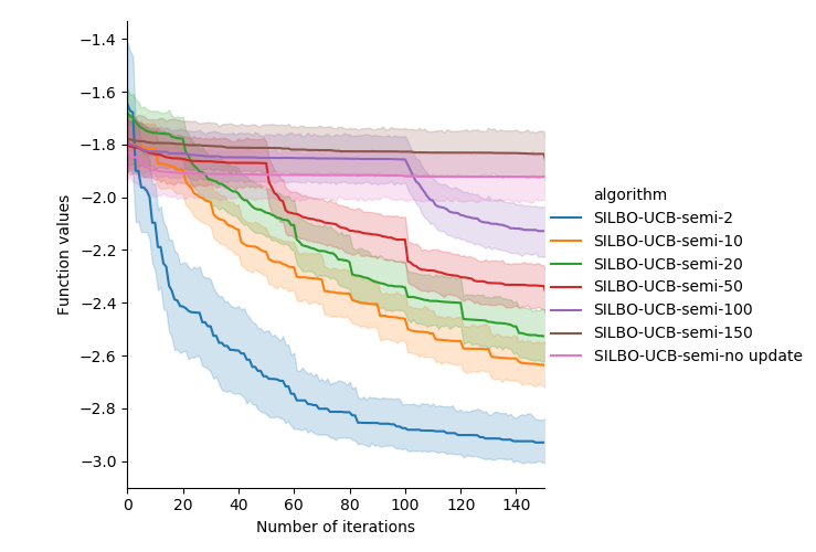
(b) 1000d Hartmann6

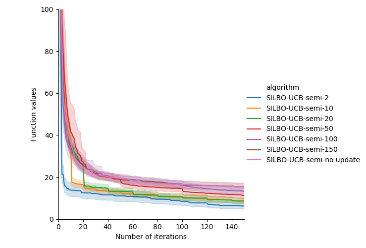
(c) 1000d Colville

Figure 11: The optimization performance of SILBO under different iterative frequency. The number represents the frequency of updating the projection matrix.

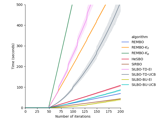
(a) 1000d Branin

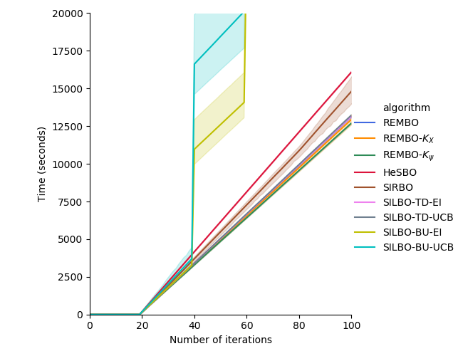
(b) 500d MLP

Figure 12: Comparison of the cumulative time on Branin with dimension 1000 and on neural network (MLP) with dimension 500.

5.6 Scalability Analysis

We analyzed the scalability by comparing the cumulative time of each algorithm under the same number of iterations. As shown in Figure 12, for low-cost objective functions such as Branin, SILBO-BU is fast, while SILBO-TD is relatively slow. This is because SILBO-TD takes a lot of time to solve the Equation 19. For expensive objective functions such as neural network, SILBO-TD takes approximately the same time as most algorithms, while SILBO-BU takes more time due to its re-evaluation procedure.

6 Conclusion and Future Work

High-dimensional Bayesian optimization is a very challenging task. To address the problem , we proposed a novel iterative embedding learning framework SILBO for high-dimensional Bayesian optimization through semi-supervised dimensional reduction. We also proposed a randomized fast algorithm for solving the embedding matrix efficiently. Moreover, according to the cost of the objective function, two different mapping strategies are proposed. Experimental results on both synthetic function and hyperparameter optimization tasks reveal that SILBO outperforms the existing state-of-the-art high-dimensional Bayesian optimization methods.

In the future, we plan to address the problem of how to determine the true dimensionality during the dimension reduction process. Moreover, we also plan to use the unlabeled information to determine the kernel hyperparameters of Gaussian process and other hyperparameters of Bayesian optimization. Also, we further plan to apply SILBO to more AutoML (Automatic Machine Learning) tasks.

Acknowledgments

This work was supported by the National Natural Science Foundation of China 
(U1811461, 61702254), National Key R&D Program of China (2019YFC1711000), Jiangsu Province Science and Technology Program (BE2017155), National Natural Science Foundation of Jiangsu Province (BK20170651), and Collaborative Innovation Center of Novel Software Technology and Industrialization.

References

- Achlioptas (2003) Dimitris Achlioptas. Database-friendly random projections: Johnson-lindenstrauss with binary coins. Journal of Computer and System Sciences, 66(4):671 – 687, 2003.
- Ailon and Chazelle (2009) Nir. Ailon and Bernard. Chazelle. The fast johnson–lindenstrauss transform and approximate nearest neighbors. SIAM Journal on Computing, 39(1):302–322, 2009.
- Belkin and Niyogi (2001) Mikhail Belkin and Partha Niyogi. Laplacian eigenmaps and spectral techniques for embedding and clustering. In Proceedings of the 14th International Conference on Neural Information Processing Systems: Natural and Synthetic, NIPS’01, page 585–591, Cambridge, MA, USA, 2001.
- Bergstra et al. (2011) James Bergstra, Rémi Bardenet, Yoshua Bengio, and Balázs Kégl. Algorithms for hyper-parameter optimization. In Proceedings of the 24th International Conference on Neural Information Processing Systems, NIPS’11, page 2546–2554, Red Hook, NY, USA, 2011.
- Binois et al. (2015) Mickaël Binois, David Ginsbourger, and Olivier Roustant. A warped kernel improving robustness in bayesian optimization via random embeddings. In Learning and Intelligent Optimization, pages 281–286, Cham, 2015.
- Binois et al. (2019) Mickaël Binois, David Ginsbourger, and Olivier Roustant. On the choice of the low-dimensional domain for global optimization via random embeddings. Journal of Global Optimization, 2019.
- Cai et al. (2007) D. Cai, X. He, and J. Han. Semi-supervised discriminant analysis. In 2007 IEEE 11th International Conference on Computer Vision, pages 1–7, Oct 2007.
- Chung (1997) F. R. K. Chung. Spectral Graph Theory. American Mathematical Society, 1997.
- Djolonga et al. (2013) Josip Djolonga, Andreas Krause, and Volkan Cevher. High-dimensional gaussian process bandits. In Advances in Neural Information Processing Systems 26, pages 1025–1033. 2013.
- Eissman et al. (2018) Stephan Eissman, Daniel Levy, Rui Shu, Stefan Bartzsch, and Stefano Ermon. Bayesian optimization and attribute adjustment. In Proc. 34th Conference on Uncertainty in Artificial Intelligence, 2018.
- Frazier (2018) Peter I. Frazier. A Tutorial on Bayesian Optimization. art. arXiv:1807.02811, 2018.
- Gardner et al. (2017) Jacob Gardner, Chuan Guo, Kilian Weinberger, Roman Garnett, and Roger Grosse. Discovering and Exploiting Additive Structure for Bayesian Optimization. In Proceedings of the 20th International Conference on Artificial Intelligence and Statistics, volume 54 of Proceedings of Machine Learning Research, pages 1311–1319, Fort Lauderdale, FL, USA, 20–22 Apr 2017.
- Georgiev and Mukherjee (2012) Stoyan Georgiev and Sayan Mukherjee. Randomized Dimension Reduction on Massive Data. art. arXiv:1211.1642, 2012.
- Gómez-Bombarelli et al. (2018) Rafael Gómez-Bombarelli, Jennifer N. Wei, David Duvenaud, José Miguel Hernández-Lobato, Benjamín Sánchez-Lengeling, Dennis Sheberla, Jorge Aguilera-Iparraguirre, Timothy D. Hirzel, Ryan P. Adams, and Alán Aspuru-Guzik. Automatic chemical design using a data-driven continuous representation of molecules. ACS Central Science, 4(2):268–276, 2018.
- Halko et al. (2011) N. Halko, P. G. Martinsson, and J. A. Tropp. Finding structure with randomness: Probabilistic algorithms for constructing approximate matrix decompositions. SIAM Review, 53(2):217–288, 2011.
- Hansen (2016) Nikolaus Hansen. The CMA Evolution Strategy: A Tutorial. arXiv e-prints, art. arXiv:1604.00772, April 2016.
- Hernández-Lobato et al. (2016) Daniel Hernández-Lobato, José Miguel Hernández-Lobato, Amar Shah, and Ryan P. Adams. Predictive entropy search for multi-objective bayesian optimization. In Proceedings of the 33rd International Conference on International Conference on Machine Learning - Volume 48, ICML’16, page 1492–1501. JMLR.org, 2016.
- Huang and Su (2014) Chiao-Ching Huang and Kuan-Ying Su. Semi-supervised dimension reduction with kernel sliced inverse regression. In Shin-Ming Cheng and Min-Yuh Day, editors, Technologies and Applications of Artificial Intelligence, pages 178–187, Cham, 2014. Springer International Publishing.
- Hutter et al. (2011) Frank Hutter, Holger H. Hoos, and Kevin Leyton-Brown. Sequential model-based optimization for general algorithm configuration. In Learning and Intelligent Optimization, pages 507–523, Berlin, Heidelberg, 2011.
- Kandasamy et al. (2015) Kirthevasan Kandasamy, Jeff Schneider, and Barnabás Póczos. High dimensional bayesian optimisation and bandits via additive models. In Proceedings of the 32nd International Conference on International Conference on Machine Learning - Volume 37, ICML’15, page 295–304, 2015.
- Kandasamy et al. (2017) Kirthevasan Kandasamy, Gautam Dasarathy, Jeff Schneider, and Barnabás Póczos. Multi-fidelity bayesian optimisation with continuous approximations. In Proceedings of the 34th International Conference on Machine Learning - Volume 70, ICML’17, page 1799–1808, 2017.
- Kandasamy et al. (2018) Kirthevasan Kandasamy, Willie Neiswanger, Jeff Schneider, Barnabás Póczos, and Eric P. Xing. Neural architecture search with bayesian optimisation and optimal transport. In Proceedings of the 32nd International Conference on Neural Information Processing Systems, NIPS’18, page 2020–2029, Red Hook, NY, USA, 2018.
- Kingma and Ba (2015) Diederik P. Kingma and Jimmy Ba. Adam: A method for stochastic optimization. In 3rd International Conference on Learning Representations, ICLR 2015, San Diego, CA, USA, May 7-9, 2015, Conference Track Proceedings, 2015.
- Klein et al. (2017) Aaron Klein, Stefan Falkner, Simon Bartels, Philipp Hennig, and Frank Hutter. Fast Bayesian Optimization of Machine Learning Hyperparameters on Large Datasets. In Aarti Singh and Jerry Zhu, editors, Proceedings of the 20th International Conference on Artificial Intelligence and Statistics, volume 54 of Proceedings of Machine Learning Research, pages 528–536, Fort Lauderdale, FL, USA, 20–22 Apr 2017. PMLR.
- Le et al. (2013) Vu Tuan Hieu Le, Cristina Stoica, T. Alamo, E.F. Camacho, and Didier Dumur. Zonotopes: From Guaranteed State Estimation to Control. Wiley-ISTE, October 2013.
- Li (1991) Ker-Chau Li. Sliced inverse regression for dimension reduction. Journal of the American Statistical Association, 86(414):316–327, 1991.
- Lu et al. (2018) Xiaoyu Lu, Javier Gonzalez, Zhenwen Dai, and Neil Lawrence. Structured variationally auto-encoded optimization. In Proceedings of the 35th International Conference on Machine Learning, volume 80 of Proceedings of Machine Learning Research, pages 3267–3275, Stockholmsmässan, Stockholm Sweden, 10–15 Jul 2018.
- Moriconi et al. (2019) Riccardo Moriconi, Marc P. Deisenroth, and K. S. Sesh Kumar. High-dimensional Bayesian optimization using low-dimensional feature spaces. arXiv e-prints, art. arXiv:1902.10675, February 2019.
- Nayebi et al. (2019) Amin Nayebi, Alexander Munteanu, and Matthias Poloczek. A framework for Bayesian optimization in embedded subspaces. In Kamalika Chaudhuri and Ruslan Salakhutdinov, editors, Proceedings of the 36th International Conference on Machine Learning, volume 97 of Proceedings of Machine Learning Research, pages 4752–4761, Long Beach, California, USA, 09–15 Jun 2019.
- Oh et al. (2018) ChangYong Oh, Efstratios Gavves, and Max Welling. Bock : Bayesian optimization with cylindrical kernels. ICML, pages 3865–3874, 2018.
- Shahriari et al. (2016) B. Shahriari, K. Swersky, Z. Wang, R. P. Adams, and N. de Freitas. Taking the human out of the loop: A review of bayesian optimization. Proceedings of the IEEE, 104(1):148–175, 2016.
- Snoek et al. (2012) Jasper Snoek, Hugo Larochelle, and Ryan P. Adams. Practical bayesian optimization of machine learning algorithms. In Proceedings of the 25th International Conference on Neural Information Processing Systems - Volume 2, NIPS’12, page 2951–2959, Red Hook, NY, USA, 2012.
- Srinivas et al. (2010) Niranjan Srinivas, Andreas Krause, Sham Kakade, and Matthias Seeger. Gaussian process optimization in the bandit setting: No regret and experimental design. In Proceedings of the 27th International Conference on International Conference on Machine Learning, ICML’10, page 1015–1022, Madison, WI, USA, 2010.
- Swersky et al. (2013) Kevin Swersky, Jasper Snoek, and Ryan P. Adams. Multi-task bayesian optimization. In Proceedings of the 26th International Conference on Neural Information Processing Systems - Volume 2, NIPS’13, page 2004–2012, Red Hook, NY, USA, 2013.
- Wang et al. (2013) Ziyu Wang, Masrour Zoghi, Frank Hutter, David Matheson, and Nando De Freitas. Bayesian optimization in high dimensions via random embeddings. In Proceedings of the Twenty-Third International Joint Conference on Artificial Intelligence, IJCAI ’13, page 1778–1784, 2013.
- Wu et al. (2017) Jian Wu, Matthias Poloczek, Andrew Gordon Wilson, and Peter I. Frazier. Bayesian optimization with gradients. In Proceedings of the 31st International Conference on Neural Information Processing Systems, NIPS’17, page 5273–5284, Red Hook, NY, USA, 2017.
- Wu et al. (2019) Jian Wu, Saul Toscano-Palmerin, I. Peter Frazier, and Gordon Andrew Wilson. Practical multi-fidelity bayesian optimization for hyperparameter tuning. UAI, 2019.
- Wu et al. (2010) Qiang Wu, Feng Liang, and Sayan Mukherjee. Localized sliced inverse regression. Journal of Computational and Graphical Statistics, 19(4):843–860, 2010.
- Zhang et al. (2019) Miao Zhang, Huiqi Li, and Steven Su. High dimensional bayesian optimization via supervised dimension reduction. In Proceedings of the Twenty-Eighth International Joint Conference on Artificial Intelligence, IJCAI-19, pages 4292–4298, 7 2019.