Mapper of Narrow Galaxy Lines (MaNGaL): new tunable filter imager for Caucasian telescopes

Abstract

We described the design and operation principles of a new tunable-filter photometer developed for the 1-m telescope of the Special Astrophysical Observatory of the Russian Academy of Sciences and the 2.5-m telescope of the Sternberg Astronomical Institute of the Moscow State University. The instrument is mounted on the scanning Fabry-Perot interferometer operating in the tunable-filter mode in the spectral range of 460-800 nm with a typical spectral resolution of about 1.3 nm. It allows one to create images of galactic and extragalactic nebulae in the emission lines having different excitation conditions and to carry out diagnostics of the gas ionization state. The main steps of observations, data calibration, and reduction are illustrated by examples of different emission-line objects: galactic H ii regions, planetary nebulae, active galaxies with extended filaments, starburst galaxies, and Perseus galaxy cluster.

1 Introduction

Tunable filter (TF) imaging systems based on low-order scanning Fabry-Perot interferometers (FPIs) have a long history of astronomical applications related to the study of extended emission-line targets: galactic and extragalactic nebulae, solar system objects Jockers1992 ; Bland1998 ; Jones2002 . The main idea of observations are well described in the above references and also illustrated in Fig. 1. If the gap between FPI plates is small and corresponds to the interference orders $n=10-30$, then it is easy to attain the FWHM of the instrumental profile $\delta\lambda=1-2$ nm. Since the distance between neighbouring interference orders (interfringe) $\Delta\lambda=\lambda/n$, we can cut the desired transmission peaks by the medium-band filter with a typical bandwidth of about 15–30 nm. The peak transmission central wavelength (CWL) can be switched between the desired emission line and neighboring continuum using a piezoelectrically-tuned and servo-stabilized FPI; the redshift/systemic velocity of the studied objects can be taken into account.

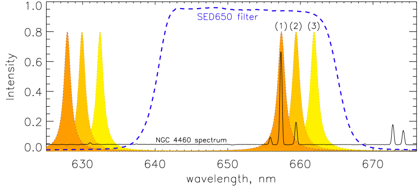
Figure 1: Tunable filter operating principle. The regions filled with various tones of orange show the transmission profiles of the FPI tuned for observations in the H$\alpha$ (1) and [N ii]$\lambda 6583$ (2) emission lines and in the continuum (3). The blue dashed line shows the transmission curve of the medium-band filter which isolates only one transmission peak of the interferometer. The parameters of FPI and medium-band filter are similar to those used in the MaNGaL; the integrated spectrum of the NGC 4460 starburst galaxy was taken from Moiseev2010 .

This technique allows us to make accurate continuum subtraction to produce pure line images and precisely distinguish the neighbouring emission lines (the H$\alpha$ and [N ii]$\lambda 6548,6583$ lines for the ionization state and metallicity diagnostics or [S ii]$\lambda 6717,6731$ lines for measurements of the electron density $n_{e}$). The last is usually impossible in the ‘traditional’ medium- or narrow-band filter imaging. From the other hand, the TF observations give a significantly large field of view (FOV) compared to the integral-field spectroscopic observations: several and even tens of arcminutes with large telescopes, whereas the integral-field system MUSE/VLT, the most powerful today, has only $1^{\prime}$ FOVMUSE . Several TF systems are in operation at large telescopes like the 6.5-m Magellan MMTF , 8.2-m SUBARU Sugai2010 , or 10.4-m GTC OSIRIS .

TFs have great research potential in observations with medium-sized telescopes and the Taurus Tunable Filter Bland1998 at the 3.9-m Anglo-Australian Telescope was the first to demonstrate this. The obtained results included the discovery of compact galaxies emitting in the H$\alpha$line at the $z\sim 0.4$ redshift Jones2001 , mapping of the extended gas around quasarsShopbell1999 , the study of meteorological processes in the atmospheres of brown dwarfs using time variability at the TiO absorption feature Tinney1999 and many other interesting findings. Nevertheless, the TF technique is not very popular now, because it is much more complicated than traditional filter imaging; moreover, some differences from ‘an ideal monochromator’ are also known. We list the problems according to Jones2002 :

1. The instrumental transmission Airy profile is more triangular rather than rectangular or Gaussian, and this complicates the flux calibration and separation of neighbouring lines.

2. Using the medium-band blocking filter limits the operating spectral range.

3. The size of the quasi-monochromatic region (Jacquinot spot) is limited, because the FPI phase changes across FOV.

In this paper, we describe the TF photometer developed for observations at Russian medium-sized telescopes, where problem (3) is partially solved by placing the FPI in the convergent beam instead of the collimated one. Also, using a large set of modern high-transparency blocking filters allows us to reduce problem (2) of the spectral range selection.

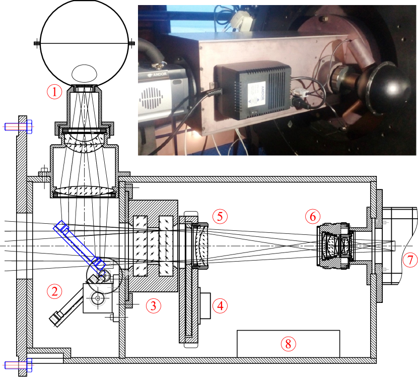
Figure 2: MaNGaL optomechanical layout and photo of the device in the Nasmyth-2 focus at the 2.5-m SAI MSU telescope. (1) – the calibration unit; (2) – the diagonal mirror; (3) – the scanning FPI; (4) – the medium-band filters wheel; (5) – the field lens; (6) – the photo lens; (7) – the CCD camera; (8) – the control computer.

2 Design of the instrument

2.1 Optical and mechanical layout

The Mapper of Narrow Galaxy Lines (MaNGaL) was developed and manufactured in the Special Astrophysical Observatory of the Russian Academy of Sciences (SAO RAS). The instrument optical scheme (Fig. 2) consists of a two-component achromatic field lens and a six-component anastigmatic photographic lens ‘Helios-44M-7’ (F/2). In contrast to the ‘classical’ optical layout having a TF in the collimated beam Jones2002 ; MMTF , MaNGaL is an afocal reducer with the FPI in the convergent beam as was proposed by Courtes Courtes1960 . This arrangement provides a significantly larger size of a central monochromatic region that is crucial in studying the extended targets. Figure 3 shows the variations of the instrumental CWL (‘phase map’, see Moiseev2002ifp ; Jones2002 ) for the same low-order FPI in two different optical schemes with the similar camera focal ratio: in the collimated beam in the SCORPIO-2 focal reducer and in MaNGaL . The figure evidences that the region, where the peak CWL changes less than $0.5\delta\lambda$, covers $\sim 90\%$ of the MaNGaL FOV, that is significantly larger than in the collimated beam. Moreover, here we use a more rigid criteria than the standard definition of the Jacquinot spot: the peak wavelength variation over the field does not exceed $\sqrt{2}\delta\lambda$ Jacquinot1954 ; Jones2002 . With this standard definition, the monochromatic spot covers the whole MaNGaL FOV. It is important to note that this optical scheme type works only with low-order interferometers, because the instrumental finesse ($\Delta\lambda/\delta\lambda$) degrades very fast with the interference order in the same convergent beam.

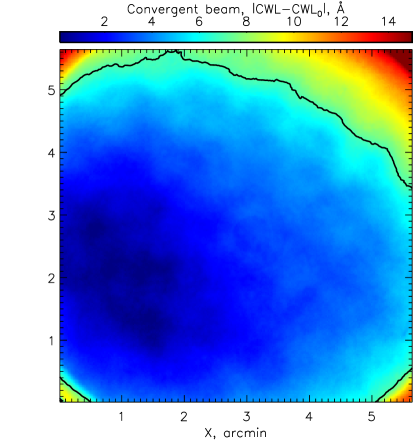
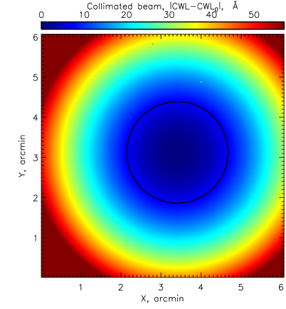
Figure 3: CWL variations across the similar field-of-view for the same low-order FPI in different optical systems. The black thick line marks the Jacquinot spot borders ($\Delta$CWL$<\frac{1}{2}\delta\lambda$). Direct measurements using the calibration lamp spectrum: FPI in the convergent beam in MaNGaL (left) and in the collimated beam in SCORPIO-2 focal reducer SCORPIO2 (right).

The mechanical part of the device also includes a USB motorized filter wheel with a changeable 5-position holder for 50-mm diameter filters produced by Edmund Optics, and a rotating diagonal mirror which directs the light from the calibration unit. The telecentric optics of the calibration unit produces an image of the area illuminated by calibration lamps in the Ulbricht integrating sphere to the entrance of the focal reducer. The focal ratio of the calibration beam is about $F/8$. The integration sphere can be illuminated by the He-Ne-Ar filled lamp (the Soviet vintage vacuum stabilitron SG3S) to calibrate the wavelength scale and the filament lamp to produce the spectral flat field.

To select the desired spectral range around the FPI transmission peak, we use hard coated bandpass filters also produced by Edmund Optics. The main set of the filters with the 25-nm bandwidth is similar to that described in Dodonov2017 . These filters uniformly cover the 460–750-nm wavelength interval, their transmission curve has an almost rectangular shape with a maximum throughput of $\sim 95\%$ (see the example in Fig. 1). Also, we use several filters with the 10-nm bandwidth which cover the spectral regions between the 25-nm filter profiles.

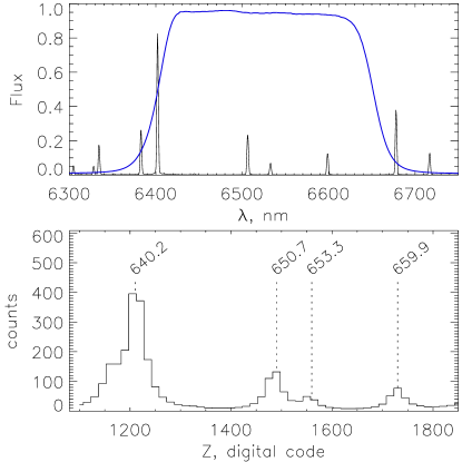
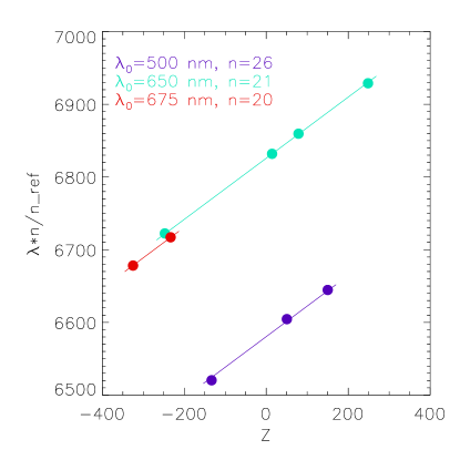
Figure 4: Left: the spectrum of the He-Ne-Ar calibration lamp, the blue line shows the transmission curve of the bandpass filter selected the 25 nm region around the H$\alpha$ line (top) and the selected spectrum scanned with the FPI (bottom). The brightest calibration lines are marked. Right: the wavelength calibration relation, different colors correspond to different spectral ranges, the CWLs of the bandpass filters are labeled, $n_{ref}=21$ .

The AVR ATtiny2313 microprocessor controls the diagonal mirror and calibration lamps, whereas the compact MR3253S-00F industrial computer is used for full control of all optical and mechanical units including the CCD camera and scanning FPI controller CS-100 (see below). The control interface for working with the local microprocessor, scanning FPI, the filter wheel, and the CCD acquisition system is written in the IDL data language.

2.2 CCD

As a detector, MaNGaL uses the iKon-M 934 camera manufactured by Andor based on a $1K\times 1K$ back-illuminated CCD optimized for the visual spectral range (QE$\geq 90\%$ in the 500–700 nm wavelength range). The camera is connected to the control computer via the USB-2 interface. The Peltier cooling system of the CCD together with the industrial chiller provide a working temperature of $-100^{\circ}$C (the coolant is the $50\%$ water-alcohol mixture). The CCD read noise is 2.5 or 6 $\mathrm{e^{-}}$, it depends on the read-out speed. The pixel scale and FOV provided by this detector at different telescopes are listed in Tab. 1.

Table 1: Main parameters of MaNGaL at the SAO RAS and SAI MSU telescopes

	1-m SAO RAS	2.5-m SAI MSU
	(Cassegrain, F/13)	(Nasmyth-2, F/8)
Total focal ratio	F/5.26	F/3.25
Field of view	$8.7^{\prime}$	$5.6^{\prime}$
Pixel scale	0.51′′	0.33′′
Spectral range	460–750 nm
Spectral resolution	1.0–1.6 nm

2.3 Scanning FPI

The ET-50 piezoelectric FPI (made by IC Optical Systems Ltd) with the appropriate characteristics was bought by SAO RAS within the project for modernization of the equipment of the 6-m SAO RAS telescope (‘the BTA Unique Scientific Instrument’). To effectively use the FPI, when it was not involved in observations at the 6-m SAO RAS telescope, it was decided to use it as a guest TF for medium-sized telescopes. The working order of interference is $n\approx 20$ (at $\lambda=656.3$ nm) that corresponds to an interferometer nominal cavity spacing of about $10\,\mu$m. The FPI reflector coating is optimized for work in the spectral range of 460–750 nm with a finesse of about $\Delta\lambda/\delta\lambda=16-27$. The corresponding typical spectral resolution is $\delta\lambda\approx 1.3\pm 0.3$ nm. Using the digital controller CS-100, we can change the gap between the interferometer plates and scanning spectra with an accuracy in wavelength of $~{}0.04$ nm.

Figure 5: Calibration relations between the actual ($r$) and the observed ($r_{obs}$) line flux ratios for the neighbouring emission line pairs: [S ii]$\lambda 6731/\lambda 6717$ (left) and [N ii]/H$\alpha$ (right). The Lorentz instrumental profile with $\delta\lambda=1.2$ nm was accepted. The solid line shows the calibration relation, whereas the dashed line corresponds to $r=r_{obs}$.

3 Wavelength calibration

In the scanning piezoelectrically-tuned interferometer, the plate spacing is changed by setting the digital value $Z_{s}$ to the CS-100 controller. In this case, the relationship between this value, wavelength, and interference order can be written as Moiseev2002ifp ; Jones2002 :

$$n\lambda=A+BZ_{s}.$$ (1)

The current order in each wavelength with the same gap is related to some ‘referred order’ $n_{ref}$ as:

$$n\lambda=n_{ref}\lambda_{ref},$$ (2)

where we accepted $\lambda_{ref}=656.3$ nm (the H$\alpha$ line). Figure 4 shows the example of the calibration lamp emission lines selected by the blocking filter and scanned with our FPI. We have 2–4 unblended calibration lines in each 25-nm blocking filter, therefore, we can determine three constants ($n_{ref}$, $A$, $B$) from (1) and (2). However, in the case of a relatively small gap (10 $\mu$m in our case), the wavelength-dependent phase change in the reflections between optical coatings on the inner plate surfaces could be important Jones2002 ; MMTF . In practice, it means that $A$ is not a constant, but depends on wavelength $A=A(\lambda)$. Therefore, we use a linear fitting of the relations ($n\lambda$ vs. $Z_{s}$) with slope $B$, but with different $A(\lambda)$ in different blocking filters. Figure 4 (right) shows the example of this fitting for the center of FOV. The shift of the filter CWL for each point across FOV is also determined from the scanning of the spectra of the same calibration lamp (see Fig. 3). The position of lines is determined using the fitting by the Lorentz contour which gives a good approximation of the FPI instrumental profile Jones2002 ; Moiseev2002ifp :

$$L(\lambda-\lambda_{0})=\frac{1}{1+\left(\frac{2(\lambda-\lambda_{0})}{\delta\lambda}\right)^{2}},$$ (3)

where $\lambda_{0}$ is a line position.

4 Data reduction

4.1 Preliminary reduction

The MaNGaL data reduction are similar to that used for ‘standard’ CCD direct-image frames. It includes: calculation and subtraction of the mean bias (with this CCD, the dark current is insufficient for typical exposures of 10-20 min), flat-field correction, and alignment of monochromatic images using the images of stars. Then we combine individual exposures at the same wavelength with the cosmic ray hits removal based on the standard sigma-clipping technique.

The flat-field frames are illuminated by the continuum spectra lamp using the same passband filter and the same scanning $Z_{S}$ values, as those of the object frames. Thanks to the relatively large Jacquinot spot, we avoid the complicated process of the removal of rings produced by the airglow night-sky emission (see Moiseev2002ifp ; Jones2002 ). Instead, in the most cases, we can accept the uniform distribution of the night-sky emission across the field.

The continuum emission is removed from the images in the lines with multiplication of the continuum frames to the coefficient $C_{cont}$ to minimize the flux residuals in the field stars. In practice, if we alternate the continuum and line exposures (see Sec. 5) and normalize the frames to the exposure time, then this coefficient is affected only by the blocking filter transmission variations and $C_{cont}\approx 1.00\pm 0.1$, because we try to avoid observations near the wings of filter transmission curve.

4.2 Flux calibration

Calibration of CCD counts to the flux in physical units [$\mbox{erg}\,\mbox{s}^{-1}\,\mbox{cm}^{-2}$] is performed according to the algorithm and equations given in Jones2002 . Briefly, we observe standard stars with the same settings (the blocking filter and $Z_{S}$) as the object frames. The expected flux from a standard star is calculated as a convolution of the tabulated star spectrum and FPI instrumental profile, that is the Lorentz profile with $\delta\lambda$ obtained from the fitting of calibration lamp lines, see (3). We observe the spectrophotometric standard stars from the ESO list which is mainly based on the data from Oke1990 . Correction for atmospheric extinction is performed with the extinction curve for the SAO RAS site Kartasheva1978 .

The detected spectrum is a product of a convolution of an actual spectrum with the instrumental profile $L(\lambda)$. If two emission lines separated in wavelength as $\Delta\lambda_{01}$ has fluxes $F_{1}$, $F_{2}$ and their ratio $r_{01}=F_{1}/F_{0}$ then our tunable filter measurement gives a smoothed observed ratio:

$$r_{obs}=\frac{F_{1}+F_{0}L(\Delta\lambda_{01})}{F_{0}+F_{1}L(\Delta\lambda_{01})}=\frac{r_{01}+L(\Delta\lambda_{01})}{1+r_{01}L(\Delta\lambda_{01})}.$$ (4)

Therefore:

$$r_{01}=\frac{r_{obs}-L(\Delta\lambda_{01})}{1-r_{obs}L(\Delta\lambda_{01})}.$$ (5)

The left-hand panel in Fig. 5 demonstrates calibration relation (5) for the case of the [S ii] doublet line ratio used for $n_{e}$ estimations.

In the case of three lines, the last equation can be written as:

$$r_{01}=\frac{r_{obs}-L(\Delta\lambda_{01})}{1+r_{12}*L(\Delta\lambda_{12})-r_{obs}[L(\Delta\lambda_{01})+C*L(\Delta\lambda_{02})]},$$ (6)

where $\Delta\lambda_{ij}=(\lambda_{i}-\lambda_{j})$. The Figure 5 (right) shows this relation for the well-known [N ii]$\lambda 6583$/H$\alpha$ line ratio, where index ‘2’ corresponds to the [N ii]$\lambda 6548$ line, and $r_{12}=1/3$.

Calibration relations (5) and (6) should be taken into account, when the corresponding line ratio maps were are created.

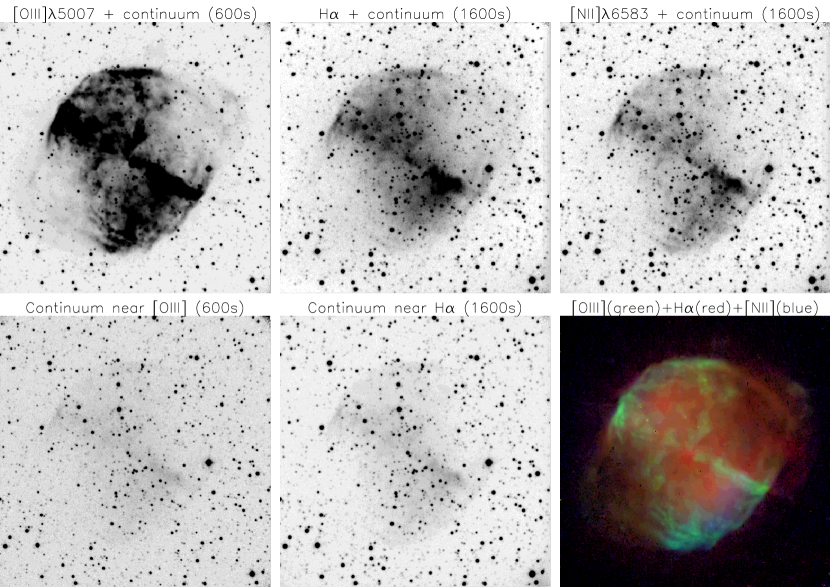
Figure 6: Images of the planetary nebula NGC 6853 (Messier 27) in the case of the FPI transmission peak centered at the emission lines and the continuum, as well as the color composite image of the nebula in the [O iii]$\lambda 5007$, H$\alpha$, and [N ii]$\lambda 6583$ lines after subtracting the stellar continuum. The total exposures are written in brackets.

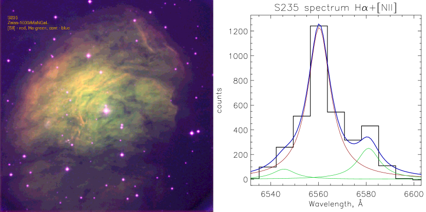
Figure 7: Observations of the Sh2-235 galactic HII region at the 1-m telescope. Left: the color composite image in the [S ii] (red), H$\alpha$ (green), and continuum (blue). Right: the example of the Lorentzian fitting of the H$\alpha$+[N ii] spectrum of the nebulae obtained with MaNGaL in the scanning mode.

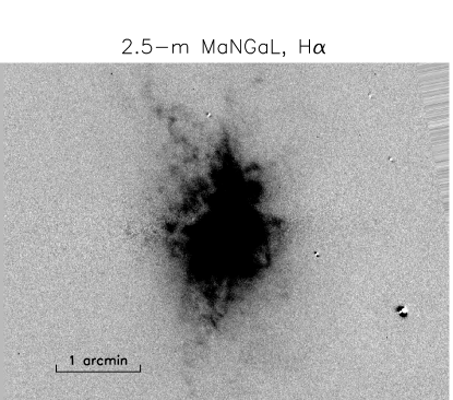
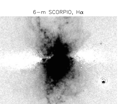
Figure 8: Continuum-subtracted H$\alpha$ images of the galactic wind in NGC 3034 (Messier 82) observed at the 2.5-m SAI MSU telescope with the tunable filter in MaNGaL (left) and the 6-m telescope data from Karachentsev2007 obtained with classical medium-band filters technique (right).

5 Observations

5.1 Main principles

Before and after an observation night, we perform the MaNGaL calibration: scanning the wavelength range in the selected bandpass filters for both He-Ne-Ar and flat-field lamps. Also, we monitor the FPI stability using a brief scan of the spectral region around the brightest calibration line in the desired filter just before the object exposure. It allows us to know the current $A$ value in equation (1).

The main mode of MaNGaL observations is the ‘TF mode’, when the CWL is tuned first to the emission line (taking into account the systemic velocity of the target and heliocentric correction), and then to the neighboring continuum (shifted by 3–5 nm). In the case of observations of the line doublets (H$\alpha$+[N ii], [S ii], etc.) the sequence can be: ‘line1–line2–continuum’. Also it is possible to observe the red and blue continuum, for example: ‘red continuum–line1–line2–blue continuum’. This cycle is repeated, which averages the variations of seeing and atmospheric extinction.

In the ‘scanning FPI mode’, we quickly scan the wavelength regions around the emission line with typical CWL increments of 0.5-0.8 nm ($\sim 0.5\delta\lambda$). In this case, we are able to obtain the low-resolution data cube to study the ionized gas kinematics and collect emission spanning a large velocity range.

5.2 SAO RAS 1-m telescope

We developed MaNGaL as a guest instrument for two medium-sized telescopes located in the Northen Caucasus region of the Russian Federation: the 1-m telescope of SAO RAS and 2.5-m telescope of the Sternberg Astronomical Institute, Lomonosov Moscow State University (SAI MSU). The parameters of the instrument at different telescopes are listed in Tab. 1.

Figure 6 demonstrates the results of the first light MaNGaL observations of the planetary nebulae Messier 27 at the Cassegrain focus of the 1-m telescope Zeiss-1000’ in September 2017: the images in the emission lines and the continuum, as well as the color composite image of the nebula in the [O iii], H$\alpha$, and [N ii] lines after subtracting the stellar continuum. The relatively large field of view in the Cassegrain focus of Zeiss-1000 is convenient for observations of galaxies having a large angular diameter and Galactic H ii regions. A good example is the Sh2-235 region of star formation, its emission-line composite image restored from MaNGaL observations is shown in Fig. 7. Also, this figure shows the spectrum in the H$\alpha$+[N ii] emission lines of this nebulae obtained in the scanning mode of MaNGaL . The detailed description and analysis of these observations are given in Kirsanova2019 .

5.3 SAI MSU 2.5-m telescope

More compact but fainter targets were observed at the 2.5-m alt-azimuthal telescope of the SAI MSU on Mt. Shatdzhatmaz Kornilov2014 . MaNGaL was mounted at the rotating stage of the Nasmyth-2 focus. An advantage of a tunable filter mapping comparing with a conventional technique of medium-band imaging is illustrated by Fig. 8. Here, the left-hand panel presents the H$\alpha$ emission line image of a prototype galactic wing nebulae in the local galaxy Messier 82 observed with MaNGaL at the 2.5-m telescope, whereas the right-hand panel shows the H$\alpha$+[N ii] view on the same region taken with at the 6-m telescope with the SCORPIO focal reducer (filter FWHMs were 7.5 nm for the emission line and 17–20 nm for the blue and red continuum). Both MaNGaL and SCORPIO data sets have a similar angular scale (0.33^′′ and 0.36^′′ per px) and total exposure (500 and 600 sec correspondingly), therefore the detected signal is significantly higher in the 6-m telescope observations, because telescope aperture and total transparency of the telescope+device system, are larger. However, using of MaNGaL allowed us to subtract very accurately the stellar host galaxy disc in contrast with the oversubtracted horizontal region in the SCORPIO data. It allows us to study weak gas emission in the region, where the underlying stellar continuum is dominated in the total spectrum.

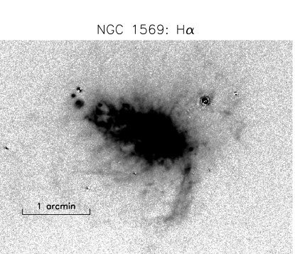
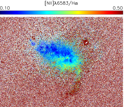
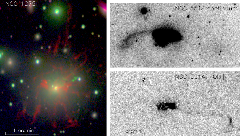
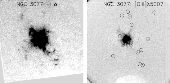
Figure 9: Various emission-line objects observed with MaNGaL at the 2.5-m SAI MSU telescope, from top to bottom: the H$\alpha$-image of the galactic wind in NGC 1569 (left) and the map of the [N ii]$\lambda$6583/H$\alpha$ ratio (right); the central galaxy of the Persieus cluster NGC 1275 (left) seen in the [N ii] (red channel), and [O iii] (green) emission lines and the images of NGC 5514 interaction pair in the continuum and in the [O iii]$\lambda 5007$ emission (right); SDSS image of the nearby dwarf galaxy NGC 3077, the MaNGaL $5.6^{\prime}$ field of view is marked (left), also the emission line images in H$\alpha$ (center) and [O iii]$\lambda 5007$ (right) are shown. Circles mark the compact emission knots – PNe candidates.

Figure 9 demonstrates the capabilities of MaNGaL  at the 2.5-m telescope for study of the ionized gas in extragalactic objects of different types:

• NGC 1569. Another example of a local starburst galaxy, where the numerous supernova explosions formed a system of suberbubbles and galactic wind outflow. The [N ii]/H$\alpha$ ratio map shows that the young stars dominate in the gas ionization in the central region ([N ii]/H$\alpha$$\approx 0.16$), whereas the shock ionization due to a galactic wind is important in the external emission filaments (those [N ii]/H$\alpha$$\geq 0.5$ are in a good agreement with previous spectral observations (see Fig. 6 in Heckman1995 ).

• NGC 1275. The [N ii] image reveals the well-known system of the ionized gas filaments extended around this central galaxy of the Perseus cluster. The [O iii] emission in the filament is very weak, it mainly comes from a high-velocity system of gaseous clouds identified as a disrupted foreground galaxy northwest of the NGC 1275 nucleus Meaburn1989 ; Boroson1990 .

• NGC 5514. A major-merger galaxy pair with a large tidal tail in the continuum image. The [O iii] map reveals for the first time the extended gaseous clouds ionized by the active nucleus at a distance of more than 60 kpc. This galaxy has been selected for MaNGaL observations as external ionized clouds candidate in the TELPERION survey Knese2020 .

• NGC 3077. The dust lanes in optical images of this dwarf starburst galaxy in the Messier 81 group are related to the ionized gas filaments Walter2002 . Our H$\alpha$ image (total exposure of 900 sec) reveals all structural features appeared in one of deepest images in the literature Karachentsev2007 . In contrast to the H$\alpha$ image, the [O iii] emission map revealed about twenty compact emission objects. The observed [O iii]/H$\alpha$ ratio allows us to consider the most of them as planetary nebulae (PNe) candidates.

Typical detection sensitivity of faint diffuse emission has been estimated in nights with photometric atmospheric conditions. At the 1-m SAO RAS telescope, the H$\alpha$ emission was detected with the signal-to-noise ratio $S/N=3$ at the $1\times 10^{-16}\,\mbox{erg}\,\mbox{s}^{-1}\,\mbox{cm}^{-2}\,\mbox{arcsec}^{-2}$ surface-brightness level (an exposure of 1200 sec, the $1\times 1$ binning mode, 26 Jan, 2018, the Sh2-235 nebulae). The corresponding value in 2.5-m telescope observations was $2\times 10^{-16}\,\mbox{erg}\,\mbox{s}^{-1}\,\mbox{cm}^{-2}\,\mbox{arcsec}^{-2}$ (an exposure of 900 sec, the $2\times 2$ binning mode, 10 Apr, 2018, the NGC 3077 galaxy).

Estimations of the MaNGaL $+2.5$-m telescope quantum efficiency (QE) and contribution of different components to the total throughput are presented in Fig. 10. The transmission curves of the optics and filters were measured in the SAO RAS laboratory; the CCD QE is given according to the manufacturer’s data. We use the direct estimation of three telescope mirrors (M1, M2 and M3) provided by the observatory staff. The prediction of the total QE telescope$+$MaNGaL in the direct-image mode (without FPI) has demonstrated a very good agreement with observations of the standard star observed in a night with photometric atmospheric conditions in Nov 2017. The total QE in the TF mode is smaller, because it includes the light lost in FPI (observations were carried out in Apr 2018). The value of total QE$=25-30\%$ is similar to that obtained with the Taurus Tunable Filter at the 3.9-m Anglo-Australian telescope Jones2002 . According to our measurements, the MaNGaL efficiency at the 1-m Ziess-1000 telescope has the same value, because its two mirrors in the Cassiegrain focus give the same losses of light as three 2.5-m telescope mirrors in its Nasmyth focus.

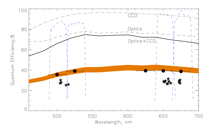
Figure 10: QE of MaNGaL at the 2.5-m telescope. Different black lines mark the transparency of different MaNGaL components according to the labels. The middle-band filters transmission curves are shown by blue lines. The orange-filled region is the total optics+telescope efficiency, its width corresponds to the mirrors’ reflecion uncertainty. The black symbols show the QE measurements using spectrophotometric standards observed without FPI (circles) and with the tunable filter (stars).

6 Conclusion

In this paper, we described the design of the MaNGaL  tunable-filter photometer and the first experience in the study of emission-line extended targets with the SAO RAS and SAI MSU medium-sized telescopes. Sciencific results published or submitted so far include the discovery of cross-ionization of gaseous discs by the active nuclei hosted in each companion galaxies in the interacting pair UGC 6081 Keel2019 , the discovery of a gaseous spiral structure in the lenticular galaxy NGC 4143 Silchenko2020 , the study of the gas ionization state in the emission filaments of NGC 3077 Oparin2020 , the reconstruction of a spatial structure of the H ii region Sh2-235 Kirsanova2019 . The most effective usage of MaNGaL consists in observation in a couple of neighbouring emission lines with different mechanism of excitation having a common point for the continuum (H$\alpha$+[N ii], e.g.). However, it also can be used to create diagnostic diagrams based on several line ratios, like [O iii]/H$\beta$ vs. [S ii]/H$\alpha$ Oparin2020 . Also, MaNGaL  is a very effective instrument in combination with other optical spectroscopic data obtained with long-slit spectrographs or high-resolution scanning Fabry-Perot interferometers, as it was shown in our works listed above.

- (1) K. Jockers, N. Thomas, T. Bonev, V. Ivanova, V. Shkodrov, Advances in Space Research 12(8), 347 (1992). DOI 10.1016/0273-1177(92)90409-Q
- (2) J. Bland-Hawthorn, D.H. Jones, PASA15, 44 (1998). DOI 10.1071/AS98044
- (3) D.H. Jones, P.L. Shopbell, J. Bland-Hawthorn, MNRAS329, 759 (2002). DOI 10.1046/j.1365-8711.2002.05001.x
- (4) A. Moiseev, I. Karachentsev, S. Kaisin, MNRAS403(4), 1849 (2010). DOI 10.1111/j.1365-2966.2010.16254.x
- (5) R. Bacon, J. Vernet, E. Borisova, N. Bouché, J. Brinchmann, M. Carollo, D. Carton, J. Caruana, S. Cerda, T. Contini, M. Franx, M. Girard, A. Guerou, N. Haddad, G. Hau, C. Herenz, J.C. Herrera, B. Husemann, T.O. Husser, A. Jarno, S. Kamann, D. Krajnovic, S. Lilly, V. Mainieri, T. Martinsson, R. Palsa, V. Patricio, A. Pécontal, R. Pello, L. Piqueras, J. Richard, C. Sandin, I. Schroetter, F. Selman, M. Shirazi, A. Smette, K. Soto, O. Streicher, T. Urrutia, P. Weilbacher, L. Wisotzki, G. Zins, The Messenger 157, 13 (2014)
- (6) S. Veilleux, B.J. Weiner, D.S.N. Rupke, M. McDonald, C. Birk, J. Bland-Hawthorn, A. Dressler, T. Hare, D. Osip, C. Pietraszewski, S.N. Vogel, AJ139, 145 (2010). DOI 10.1088/0004-6256/139/1/145
- (7) H. Sugai, T. Hattori, A. Kawai, S. Ozaki, T. Hayashi, T. Ishigaki, M. Ishii, H. Ohtani, A. Shimono, Y. Okita, K. Matsubayashi, G. Kosugi, M. Sasaki, N. Takeyama, PASP122(887), 103 (2010). DOI 10.1086/650397
- (8) J.J. González, J. Cepa, J.I. González-Serrano, M. Sánchez-Portal, MNRAS443, 3289 (2014). DOI 10.1093/mnras/stu1310
- (9) D.H. Jones, J. Bland-Hawthorn, ApJ550(2), 593 (2001). DOI 10.1086/319793
- (10) P.L. Shopbell, S. Veilleux, J. Bland-Hawthorn, ApJLett524(2), L83 (1999). DOI 10.1086/312311
- (11) C.G. Tinney, A.J. Tolley, MNRAS304(1), 119 (1999). DOI 10.1046/j.1365-8711.1999.02297.x
- (12) G. Courtès, Annales d’Astrophysique 23, 115 (1960)
- (13) A.V. Moiseev, Bulletin of the Special Astrophysics Observatory 54, 74 (2002)
- (14) P. Jacquinot, Journal of the Optical Society of America (1917-1983) 44(10), 761 (1954)
- (15) V.L. Afanasiev, A.V. Moiseev, Baltic Astronomy 20, 363 (2011)
- (16) S.N. Dodonov, S.S. Kotov, T.A. Movsesyan, M. Gevorkyan, Astrophysical Bulletin 72(4), 473 (2017). DOI 10.1134/S1990341317040113
- (17) J.B. Oke, AJ99, 1621 (1990). DOI 10.1086/115444
- (18) T.A. Kartasheva, N.M. Chunakova, Astrofizicheskie Issledovaniia Izvestiya Spetsial’noj Astrofizicheskoj Observatorii 10, 44 (1978)
- (19) I.D. Karachentsev, S.S. Kaisin, AJ133, 1883 (2007). DOI 10.1086/512127
- (20) M.S. Kirsanova, P.A. Boley, A.V. Moiseev, D.S. Wiebe, R.I. Uklein, MNRAS497(1), 1050 (2020). DOI 10.1093/mnras/staa2004
- (21) V. Kornilov, B. Safonov, M. Kornilov, N. Shatsky, O. Voziakova, S. Potanin, I. Gorbunov, V. Senik, D. Cheryasov, PASP126(939), 482 (2014). DOI 10.1086/676648
- (22) T.M. Heckman, M. Dahlem, M.D. Lehnert, G. Fabbiano, D. Gilmore, W.H. Waller, ApJ448, 98 (1995). DOI 10.1086/175944
- (23) J. Meaburn, P.M. Allan, C.A. Clayton, A.P. Marston, M.J. Whitehead, A. Pedlar, A&A208, 17 (1989)
- (24) T.A. Boroson, ApJ360, 465 (1990). DOI 10.1086/169136
- (25) E.D. Knese, W.C. Keel, G. Knese, V.N. Bennert, A. Moiseev, A. Grokhovskaya, S.N. Dodonov, MNRAS496(2), 1035 (2020). DOI 10.1093/mnras/staa1510
- (26) F. Walter, A. Weiss, C. Martin, N. Scoville, AJ123, 225 (2002). DOI 10.1086/324633
- (27) W.C. Keel, V.N. Bennert, A. Pancoast, C.E. Harris, A. Nierenberg, S.D. Chojnowski, A.V. Moiseev, D.V. Oparin, C.J. Lintott, K. Schawinski, G. Mitchell, C. Cornen, MNRAS483(4), 4847 (2019). DOI 10.1093/mnras/sty3332
- (28) O.K. Sil’chenko, A.V. Moiseev, D. Oparin, Astronomy Letters accepted (2020)
- (29) D.V. Oparin, O.V. Egorov, A.V. Moiseev, Astrophysical Bulletin accepted (2020)