Predicting Dynamics on Networks Hardly Depends on the Topology

Abstract

Processes on networks consist of two interdependent parts: the network topology, consisting of the links between nodes, and the dynamics, specified by some governing equations. This work considers the prediction of the future dynamics on an unknown network, based on past observations of the dynamics. For a general class of governing equations, we propose a prediction algorithm which infers the network as an intermediate step. Inferring the network is impossible in practice, due to a dramatically ill-conditioned linear system. Surprisingly, a highly accurate prediction of the dynamics is possible nonetheless: Even though the inferred network has no topological similarity with the true network, both networks result in practically the same future dynamics.

1 Introduction

The interplay of dynamics and structure lies at the heart of myriad processes on networks, ranging from predator-prey interactions on ecological networks [1] and epidemic outbreaks on physical contact networks [2] to brain activity on neural networks [3]. To relate the network structure and the process dynamics, there are two approaches of opposing directions. On the one hand, a great body of research [4, 5, 6] focusses on the question: What is the impact of the network structure on the dynamics of a process? For instance, the impact of the network of online social media friendships on the spread of fake news. On the other hand, network reconstruction methods [7, 8, 9, 10] consider the inverse problem: Given some observations of dynamics, what can we infer about the network structure? As an example, one may ask to determine the path of an infectious virus from one individual to another, given observations of the epidemic outbreak.

The prediction of dynamics on an unknown network seems to require the combination of both directions: first, the reconstruction of the network structure based on past observations of the dynamics and, second, the estimation of the future dynamics based on the inferred (i.e. reconstructed) network. Intuitively, one may expect that an accurate prediction of the dynamics is possible only if the network reconstruction is accurate. In this work, paradoxically, we show the contrary: it is possible to accurately predict a general class of dynamics without the network structure.

2 Modelling Dynamics on Networks

The network is represented by the $N\times N$ weighted adjacency matrix $A$ whose elements are denoted by $a_{ij}$. If there is a directed link from node $j$ to node $i$, then it holds that $a_{ij}>0$, and $a_{ij}=0$ otherwise. Throughout this work, we make a clear distinction between the network topology and the interaction strengths [11]. The network topology, or network structure, is the set of all links: all node pairs $(i,j)$ for which $a_{ij}>0$. If there is a link from node $j$ to node $i$, then the interaction strength is specified by the link weight $a_{ij}$. For instance, consider the two $3\times 3$ adjacency matrices

$$A=\begin{pmatrix}0&1&0\\ 2&0&0\\ 0&2&2\end{pmatrix},\quad\hat{A}=\begin{pmatrix}0&2&0\\ 1&0&0\\ 0&2&3\end{pmatrix}.$$

For all nodes $i,j$, it holds that $a_{ij}>0$ if and only if $\hat{a}_{ij}>0$. Hence, the two matrices $A$ and $\hat{A}$ have the same network topology. However, the interaction strength, e.g., from node 2 to node 1 is different, because $a_{12}=1$ but $\hat{a}_{12}=2$.

We denote the nodal state of node $i$ at time $t$ by $x_{i}(t)$ and the nodal state vector by $x(t)=(x_{1}(t),...,x_{N}(t))^{T}$. We consider a general class of dynamical models on networks [12, 7, 13] that describe the evolution of the nodal state $x_{i}(t)$ of any node $i$ as

$$\frac{dx_{i}(t)}{dt}=f_{i}\left(x_{i}(t)\right)+\sum^{N}_{j=1}a_{ij}g\left(x_{i}(t),x_{j}(t)\right).$$ (1)

The function $f_{i}\left(x_{i}(t)\right)$ describes the self-dynamics of node $i$. The sum in (1) represents the interactions of node $i$ with its neighbours. The interaction between two nodes $i$ and $j$ depends on the adjacency matrix $A$ and the interaction function $g\left(x_{i}(t),x_{j}(t)\right)$. A broad spectrum of models follows from (1) by specifying the self-dynamics function $f_{i}$ and the interaction function $g$. We study six particular models of dynamics on networks, which are summarised by Table 1:

Model	$f_{i}\left(x_{i}(t)\right)$	$g\left(x_{i}(t),x_{j}(t)\right)$
Lotka-Volterra (LV)	$x_{i}(t)(\alpha_{i}-\theta_{i}x_{i}(t))$	$-x_{i}(t)x_{j}(t)$
Mutualistic population (MP)	$x_{i}(t)(\alpha_{i}-\theta_{i}x_{i}(t))$	$x_{i}(t)x^{2}_{j}(t)(1+x^{2}_{j}(t))^{-1}$
Michaelis-Menten (MM)	$-x_{i}(t)$	$x^{h}_{j}(t)(1+x^{h}_{j}(t))^{-1}$
SIS epidemics (SIS)	$-\delta_{i}x_{i}(t)$	$(1-x_{i}(t))x_{j}(t)$
Kuramoto (KUR)	$\omega_{i}$	$\sin\left(x_{i}(t)-x_{j}(t)\right)$
Cowan-Wilson (CW)	$-x_{i}(t)$	$\left(1+\exp\left(-\tau(x_{j}(t)-\mu)\right)\right)^{-1}$

Table 1: Models of dynamics on networks.

Lotka-Volterra population dynamics (LV)

The Lotka-Volterra model [14] describes the population dynamics of competing species. The nodal state $x_{i}(t)$ denotes the population size of species $i$, the growth parameters of species $i$ equal $\alpha_{i}>0$ and $\theta_{i}>0$, and the link weight $a_{ij}$ quantifies the competition rate, or predation rate, of species $j$ on species $i$.

Mutualistic population dynamics (MP)

We adopt the model of Harush and Barzel [15] to describe mutualistic population dynamics. The nodal state $x_{i}(t)$ denotes the population size of species $i$, the growth parameters of species $i$ are denoted by $\alpha_{i}>0$ and $\theta_{i}>0$, and the link weight $a_{ij}>0$ quantifies the strength of mutualism between species $i$ and species $j$.

Michaelis-Menten regulatory dynamics (MM)

The dynamics of gene regulatory networks can be described by the Michaelis-Menten equation [16, 17, 15]. The nodal state $x_{i}(t)$ is the expression level of gene $i$, the Hill coefficient is denoted by $h$, and the link weights $a_{ij}>0$ are the reaction rate constants.

Susceptible-Infected-Susceptible epidemics (SIS)

Spreading phenomena, such as the epidemic of an infectious disease, can be described by the susceptible-infected-susceptible model [18, 19, 20, 2]. The nodal state $x_{i}(t)$ equals the infection probability of node $i$. The parameter $\delta_{i}>0$ denotes the curing rate, and the link weight $a_{ij}$ is the infection rate from node $j$ to node $i$.

Kuramoto oscillators (KUR)

The Kuramoto model [21] has been applied to various synchronisation phenomena of phase oscillators, such as fMRI activity of brain regions [3]. Here, the nodal state $x_{i}(t)$ corresponds to the phase of oscillator $i$, the parameter $\omega_{i}$ denotes the natural frequency of node $i$, and the coupling strength from node $j$ to node $i$ is given by the link weight $a_{ij}$.

Cowan-Wilson neural firing (CW)

The firing-rates of neurons can be described by the Cowan-Wilson model [22, 13]. Here, the nodal state $x_{i}(t)$ is the activity of neuron $i$, and the parameters $\tau$ and $\mu$ are the slope and the threshold of the neural activation function. The link weight $a_{ij}$ specifies the number and strength of synapses from neuron $j$ to neuron $i$.

As stated in [23], there are three possibilities for the qualitative long-term behaviour of the dynamical system (1). First, the nodal state $x(t)$ might approach a steady state $x_{\infty}=\underset{t\rightarrow\infty}{\operatorname{lim}}~{}x(t)$. At the steady state $x_{\infty}$, the nodal state does not change any longer, and it holds that $dx(t)/dt=0$. Second, the nodal state $x(t)$ might converge to a limit cycle, a curve on which the nodal state $x(t)$ circulates forever. Third, the nodal state $x(t)$ might never come to rest nor enter a repeating cycle. Then, the state $x(t)$ perpetually continues to move in an irregular pattern.

3 Prediction Algorithm for Dynamics on Networks

The true adjacency matrix $A$ is unknown. To predict the nodal state $x(t)$, we obtain an estimate $\hat{A}$ of the matrix $A$ from past observations of the nodal state $x(t)$. With the estimated matrix $\hat{A}$, we can approximate the governing equations (1) for the nodal state $x(t)$. Figure 1 illustrates the framework for predicting network dynamics.

(a) Observation

(b) Reconstructed network

(c) Prediction

Figure 1: Framework for Predicting Dynamics on Networks. This example shows a small network of $N=3$ nodes. (a) The nodal state $x_{i}(t)$ is observed for all nodes $i$ until the observation time $t_{\textrm{obs}}=2$. The evolution of the state $x_{i}(t)$ follows from the system (1) with the known functions $f_{i}$, $g$ and the unknown adjacency matrix $A$. (b) From the nodal state observations, we infer an estimate $\hat{A}$ for the true adjacency matrix $A$ by the LASSO (6). (c) For any time $t\geq t_{\textrm{obs}}$, the predicted nodal state $\hat{x}_{i}(t)$ follows from the system (1) by replacing the true adjacency matrix $A$ with the estimate $\hat{A}$. The predicted nodal state is initialised as $\hat{x}_{i}(t_{\textrm{obs}})=x_{i}(t_{\textrm{obs}})$ for all nodes $i$.

We consider $n+1$ nodal state observations $x(0),x(\Delta t),...,x(n\Delta t)$ from the initial time $t=0$ until the observation time $t=t_{\textrm{obs}}$. Here, $\Delta t>0$ denotes the sampling time with $n\Delta t=t_{\textrm{obs}}$. For a sufficiently small sampling time $\Delta t$, the solution of the model (1) obeys

$$x_{i}\left((k+1)\Delta t\right)\approx x_{i}\left(k\Delta t\right)+\Delta t\left.\frac{dx_{i}(t)}{dt}\right|_{t=k\Delta t}$$ (2)

at every time $k=0,...,n-1$. A crucial observation is that the derivative $dx_{i}(t)/dt$ in (1) is linear with respect to the entries $a_{ij}$ of the adjacency matrix $A$. Thus, we obtain from (1) and the discrete-time approximation (2) an approximate linear system as

$$V_{i}\approx F_{i}\begin{pmatrix}a_{i1}\\ \vdots\\ a_{iN}\end{pmatrix},$$ (3)

where the $n\times 1$ vector $V_{i}$ equals

$$V_{i}=\begin{pmatrix}\dfrac{x_{i}\left(\Delta t\right)-x_{i}\left(0\right)}{\Delta t}-f_{i}(0)\\ \vdots\\ \dfrac{x_{i}\left(n\Delta t\right)-x_{i}\left((n-1)\Delta t\right)}{\Delta t}-f_{i}((n-1)\Delta t)\end{pmatrix},$$ (4)

and the $n\times N$ matrix $F_{i}$ equals

$$F_{i}=\begin{pmatrix}g(x_{i}(0),x_{1}(0))&...&g(x_{i}(0),x_{N}(0))\\ \vdots&\ddots&\vdots\\ g(x_{i}((n-1)\Delta t),x_{1}((n-1)\Delta t))&...&g(x_{i}((n-1)\Delta t),x_{N}((n-1)\Delta t))\end{pmatrix}.$$ (5)

From (3), we obtain an estimate $\hat{A}$ of the adjacency matrix $A$ by solving

$$\begin{aligned} &\underset{a_{i1},...,a_{iN}}{\text{min}}&&\left\lVert V_{i}-F_{i}\begin{pmatrix}a_{i1}\\ \vdots\\ a_{iN}\end{pmatrix}\right\rVert^{2}_{2}+\rho_{i}\sum^{N}_{j=1}a_{ij}&\\ &\text{s.t.}&&a_{ij}\geq 0\quad j=1,...,N&\end{aligned}$$ (6)

for every node $i$. The optimisation problem (6) is known as the least absolute shrinkage and selection operator (LASSO) [24]. The application of LASSO, and variations thereof, to network reconstruction is an established approach [25, 7, 8, 26]. The first addend in (6) measures the consistency of the link weights $a_{i1}$, …, $a_{iN}$ with the observations $x(0),...,x(n\Delta t)$, given the dynamical model (1). The second addend favours a sparse solution. The greater the regularisation parameter $\rho_{i}>0$, the sparser the reconstructed adjacency matrix $\hat{A}$. We set the value of the parameter $\rho_{i}$ by hold-out cross-validation [27]. The LASSO (6) can be interpreted as Bayesian estimation problem, provided an exponential prior degree distribution of the adjacency matrix $A$. For more details on the reconstruction algorithm and the Bayesian interpretation, we refer the reader to Appendix A.

4 The Prediction Accuracy versus the Reconstruction Accuracy

To evaluate the prediction algorithm outlined in Section 3, we consider the dynamics in Table 1 on the respective real-world networks: (LV) Food web of Little Rock Lake [28], (MP) Mutualistic insect interactions [29, 30], (MM) Gene regulatory network of the yeast S. Cerevisiae [31], (SIS) Face-to-face contacts between visitors of the “Infectious: stay away exhibition” [32], (KUR) Structural connectivity between brain regions [33, 34], (CW) C. elegans neuronal connectivity [35, 36]. Appendix B specifies the real-world networks and model parameters in detail.

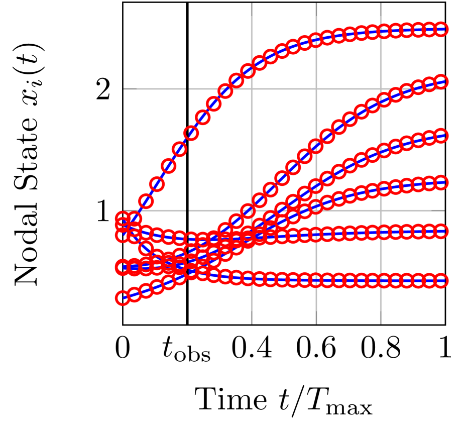
(a) LV ($N=183$)

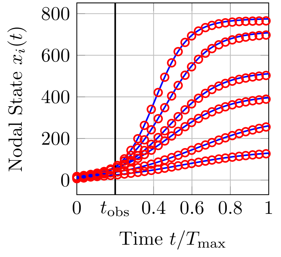
(b) MP ($N=679$)

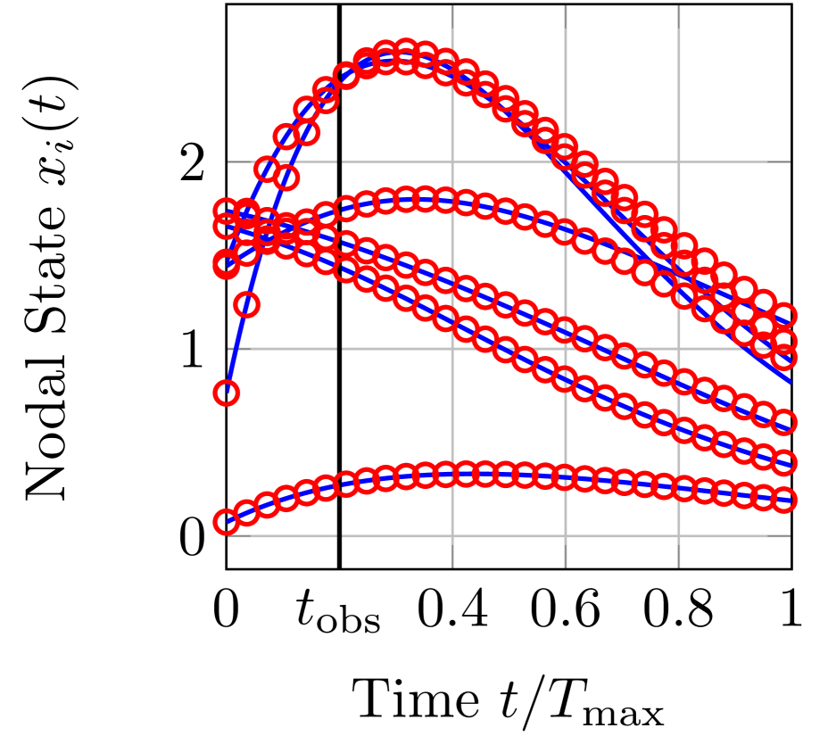
(c) MM ($N=620$)

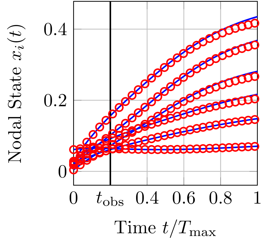
(d) SIS ($N=410$)

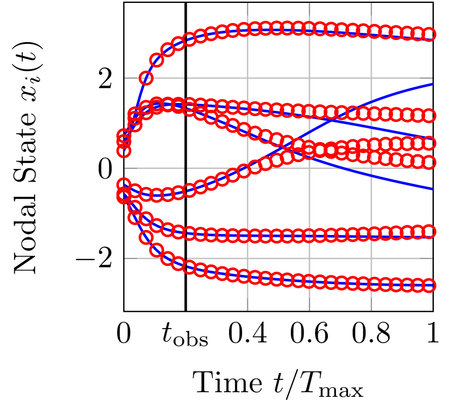
(e) KUR ($N=78$)

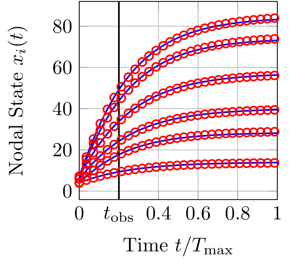
(f) CW ($N=282$)

Figure 2: Prediction Accuracy of Network Dynamics. The blue curves are the true nodal states $x_{i}(t)$. The red marks are the nodal states $\hat{x}_{i}(t)$ on the reconstructed network $\hat{A}$, initialised at $\hat{x}(0)=x(0)$ and $\hat{x}(t_{\textrm{obs}})=x(t_{\textrm{obs}})$ for the time intervals $t<t_{\textrm{obs}}$ and $t\geq t_{\textrm{obs}}$, respectively. For readability, only six nodal states $x_{i}(t)$ are depicted for each network. The maximum prediction time $T_{\textrm{max}}$ is different for each dynamic model, and the observation time equals $t_{\textrm{obs}}=T_{\textrm{max}}/5$. The number of observations is $n=100$.

Figure 2 shows that the nodal state prediction $\hat{x}(t)$ is accurate at all times $t\geq t_{\textrm{obs}}$, except for the Kuramoto model. The Kuramoto nodal state prediction $\hat{x}(t)$ is accurate from time $t=t_{\textrm{obs}}$ until $t\approx 2t_{\textrm{obs}}$, but then diverges from the true nodal state $x(t)$. In Section 5, we explain what makes the Kuramoto model different.

In view of the high prediction accuracy, we face the fundamental question: How similar are the topologies of the estimated network $\hat{A}$ and the true network $A$? We quantify the similarity of the networks $A$ and $\hat{A}$ by two topological metrics. First, we consider the area under the receiver-operating-characteristic curve (AUC) [37]. An AUC of 0.5 corresponds to reconstructing the network by tossing a coin for every possible link. The closer the AUC is to 1, the greater the similarity of the reconstructed topology to the true topology. Second, we consider the in-degree distribution of the matrices $A$ and $\hat{A}$. The in-degree $d_{i}$ of node $i$ equals the number of links that end at node $i$. The in-degree distribution is given by $\operatorname{Pr}\left[D\geq d\right]$, where $D$ is the degree of a randomly chosen node in the network.

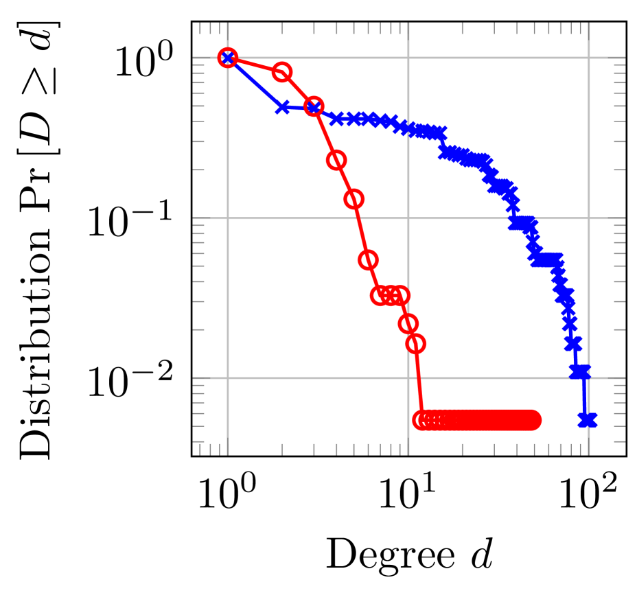
(a) LV: AUC=0.52

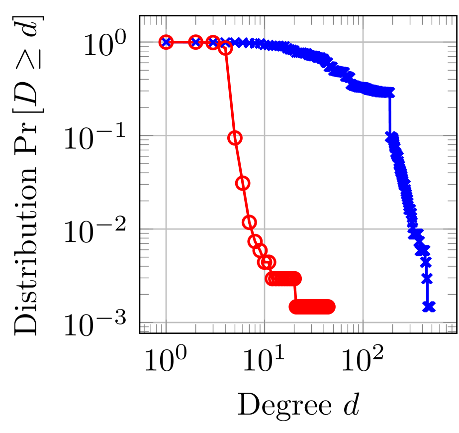
(b) MP: AUC=0.51

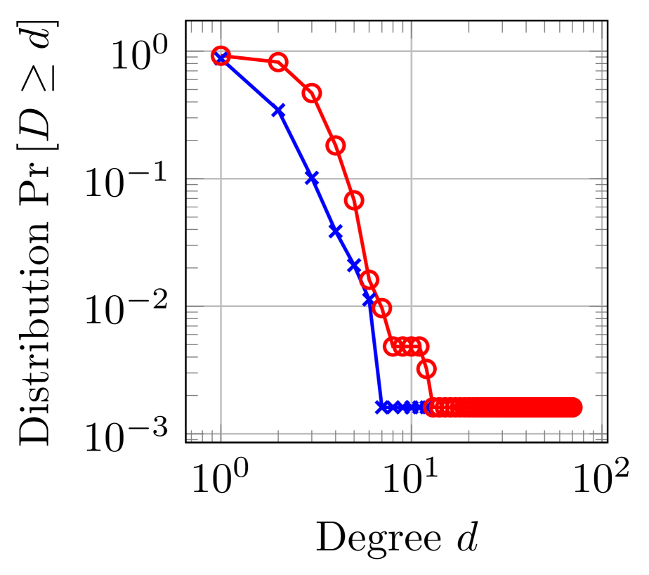
(c) MM: AUC=0.57

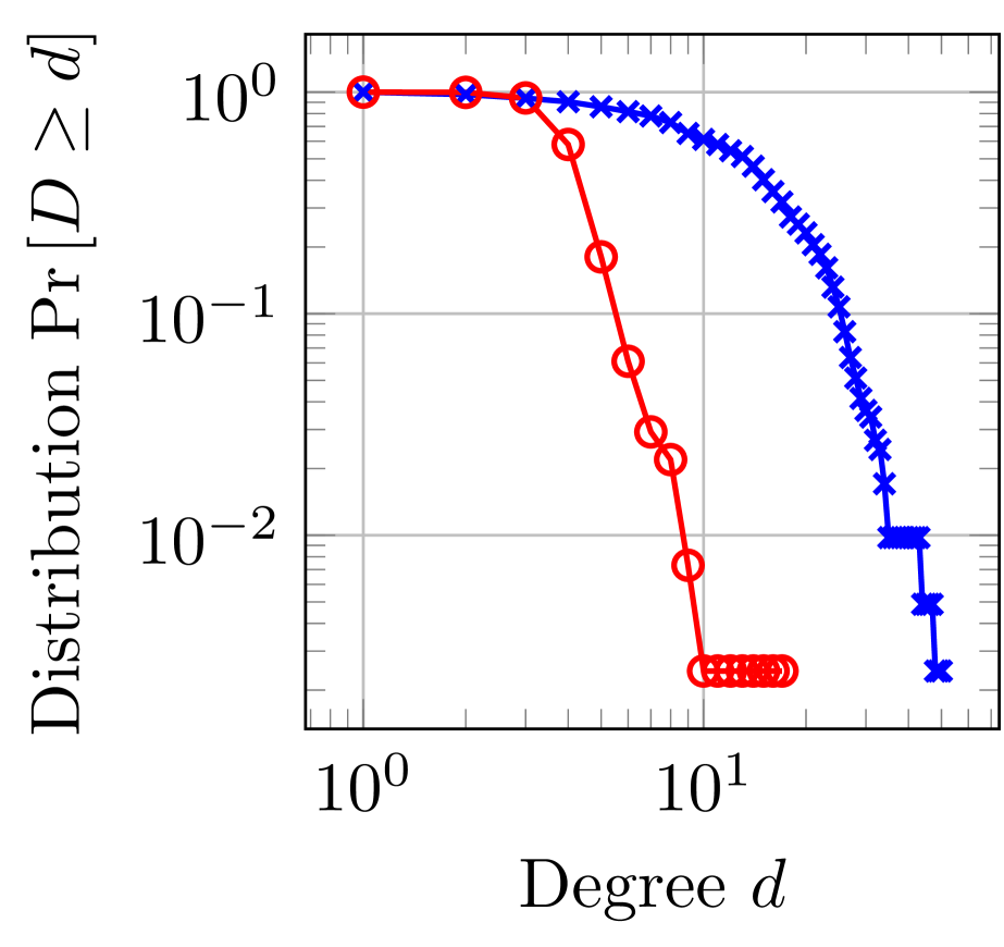
(d) SIS: AUC=0.52

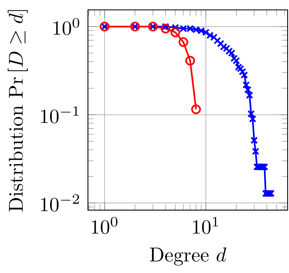
(e) KUR: AUC=0.54

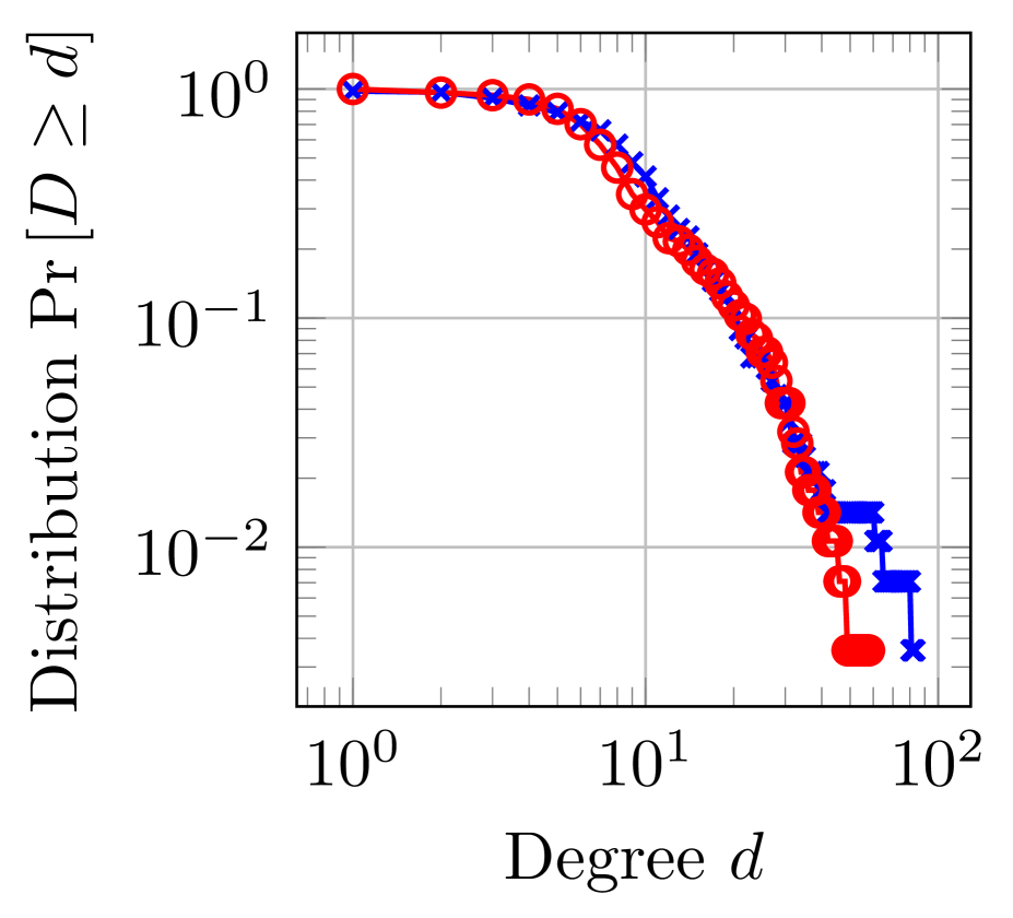
(f) CW: AUC=0.53

Figure 3: Network Reconstruction Accuracy. The reconstruction accuracy for the networks in Figure 2 with respect to two topological metrics. First, the AUC value of the reconstructed network $\hat{A}$. Second, the in-degree distributions $\operatorname{Pr}\left[D\geq d\right]$ for the estimated matrix $\hat{A}$ in red and the true matrix $A$ in blue.

Figure 3 compares the reconstructed network $\hat{A}$ to the true network $A$. The AUC value is close to 0.5 for all models. Hence, the topology of the reconstructed network bears practically no resemblance to the true network topology. Moreover, the degree distribution $\operatorname{Pr}\left[D\geq d\right]$ of the reconstructed network differs strongly to the degree distribution of the true network, except for Figure 3(c) and Figure 3(f). We emphasise that, even if two networks have the same degree distribution $\operatorname{Pr}\left[D\geq d\right]$, the network topologies can be entirely different. For instance, the AUC value equals only 0.53 in Figure 3(f).

5 Proper Orthogonal Decomposition of the Nodal State Dynamics

The dramatic contrast of accurate prediction of dynamics but inaccurate network reconstruction demands an explanation. The sole input to the prediction algorithm are the observations of the nodal state $x(t)$, which has two implications. First, the nodal state sequence $x(0),...,x(n\Delta t)$ does not contain sufficient information to infer the network topology. Second, we do not need the topology to predict the nodal state $x(t)$. But, if not the topology, what else is required to accurately predict dynamics on networks?

Example 1.

Consider a small network of $N=3$ nodes with the weighted adjacency matrix

$$A=\begin{pmatrix}0&0&2\\ 1&0&3\\ 0&1&1\end{pmatrix}.$$

Suppose that the nodal state vector equals $x(t)=(c_{1}(t),c_{2}(t),c_{2}(t))^{T}$ at every time $t$, where $c_{1}(t)$ and $c_{2}(t)$ denote some scalar functions. In other words, node 2 and node 3 have the same state at every time $t$. As vector equation, the nodal state $x(t)$ satisfies

$$x(t)=c_{1}(t)\begin{pmatrix}1\\ 0\\ 0\end{pmatrix}+c_{2}(t)\begin{pmatrix}0\\ 1\\ 1\end{pmatrix}.$$ (7)

For simplicity, we only consider the estimation of the links to node 1, i.e., $a_{11}$, $a_{12}$ and $a_{13}$. The evolution of the nodal state $x_{1}(t)$ follows from the dynamical model (1) as

$$\frac{dx_{1}(t)}{dt} =f_{1}(x_{1}(t))+2g(x_{1}(t),x_{3}(t)).$$

However, since $x_{2}(t)=x_{3}(t)=c_{2}(t)$ at every time $t$, it also holds that

$$\frac{dx_{1}(t)}{dt} =f_{1}(x_{1}(t))+2g(x_{1}(t),x_{2}(t)).$$

Thus, if we estimated the adjacency matrix $\hat{A}$ with $\hat{a}_{11}=0$, $\hat{a}_{12}=2$ and $\hat{a}_{13}=0$, then we could perfectly predict the nodal state $x_{1}(t)$. But neither estimate $\hat{a}_{12}$ nor $\hat{a}_{13}$ is equal to the true link weights $a_{12}$ and $a_{13}$, respectively.

For Example 1, the estimate $\hat{A}$ yields a perfect prediction of the dynamics, because $2g(x_{1}(t),x_{3}(t))=2g(x_{1}(t),x_{2}(t))$. More generally, the estimated network $\hat{A}$ predicts the dynamics (1) exactly if and only if, at every future time $t\geq t_{\textrm{obs}}$,

$$\sum^{N}_{j=1}\hat{a}_{ij}g\left(x_{i}(t),x_{j}(t)\right)=\sum^{N}_{j=1}a_{ij}g\left(x_{i}(t),x_{j}(t)\right).$$ (8)

The network topology of the estimate $\hat{A}$ is relevant for predicting the dynamics only if the topology relates to (8). We emphasise that (8) is linear with respect to the matrix $\hat{A}$ but not linear with respect to the nodal state $x(t)$, unless the interaction function $g$ is linear.

In Example 1, there exists a matrix $\hat{A}\neq A$ that satisfies (8), because the $3\times 1$ nodal state vector $x(t)$ is equal to the linear combination (7) of only 2 orthogonal vectors $y_{1}=(1,0,0)^{T}$ and $y_{2}=(0,1,1)^{T}$. In general, it is possible to approximate any $N\times 1$ nodal state vector $x(t)$ by

$$x(t)\approx\sum^{m}_{p=1}c_{p}(t)y_{p}$$ (9)

at every time $t\in[0,T_{\textrm{max}}]$. Here, the agitation modes $y_{1},...,y_{m}$ are some orthogonal vectors. The approximation (9) is known as proper orthogonal decomposition [38, 39]. The more agitation modes $m$, the more accurate the approximation (9). If $m=N$, then the approximation (9) is exact, because any $N\times 1$ vector $x(t)$ can be written as the linear combination of $N$ orthogonal vectors. Intuitively speaking, if the proper orthogonal decomposition (9) is accurate for $m<<N$ modes, then the nodal state vector $x(t)$ is barely agitated.

In contrast to the zero-one vectors in Example 1, the agitation modes $y_{p}$ are usually more complicated. We obtain the agitation modes $y_{p}$ from the observations of the nodal state dynamics in two steps. First, we define the $N\times(n+1)$ nodal state matrix as

$$X=\begin{pmatrix}x(0)&x(\Delta t)&...&x(n\Delta t)\end{pmatrix}.$$

Second, we obtain the agitation modes $y_{1},...,y_{m}$ as the first $m$ left-singular vectors of the nodal state matrix $X$. At any time $t\geq 0$, the scalar functions $c_{p}(t)$ follow as the inner product

$$c_{p}(t)=y^{T}_{p}x(t).$$

Figure 4 shows that the proper orthogonal decomposition (9) is accurate at all times $t\in[0,T_{\textrm{max}}]$. The number of agitation modes $y_{p}$ equals $m=15$, which is considerably lower than the network size $N$. We emphasise that the agitation modes $y_{p}$ are computed from the nodal state $x(t)$ only until the observation time $t_{\textrm{obs}}$. Nevertheless, the proper orthogonal decomposition is accurate also at times $t\geq t_{\textrm{obs}}$. Hence, during the observation interval $[0,t_{\textrm{obs}}]$, the nodal state $x(t)$ quickly locks into only few agitation modes $y_{p}$, which govern the dynamics also for future time $t\geq t_{\textrm{obs}}$. For clarity, we stress that the proper orthogonal decomposition (9) cannot be used (directly) to predict the nodal state $x(t)$: Additionally to the agitation modes $y_{p}$, the coefficients $c_{p}(t)$ at times $t\geq t_{\textrm{obs}}$ require the future nodal state $x(t)$.

(a) LV ($N=183$)

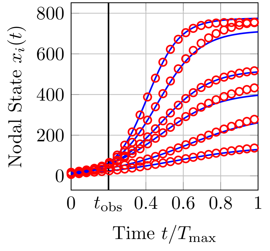
(b) MP ($N=679$)

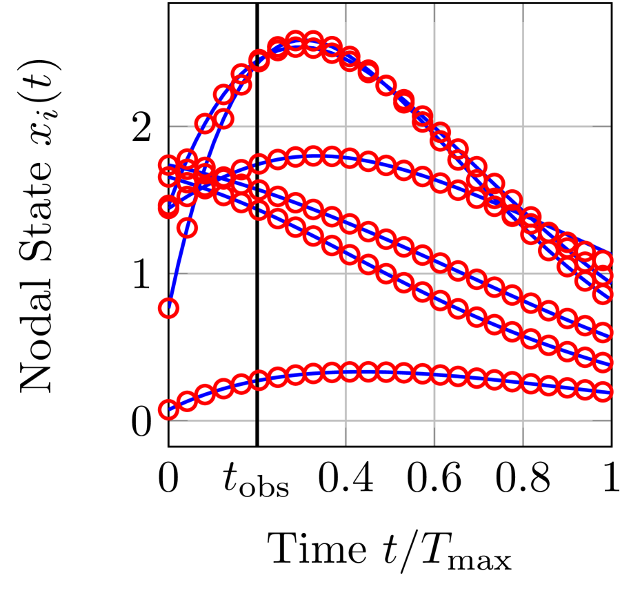
(c) MM ($N=620$)

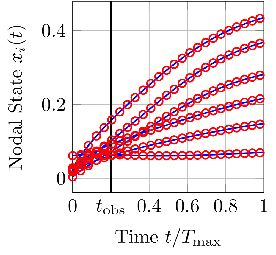
(d) SIS ($N=410$)

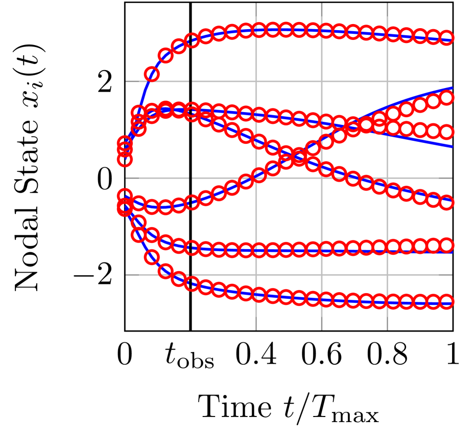
(e) KUR ($N=78$)

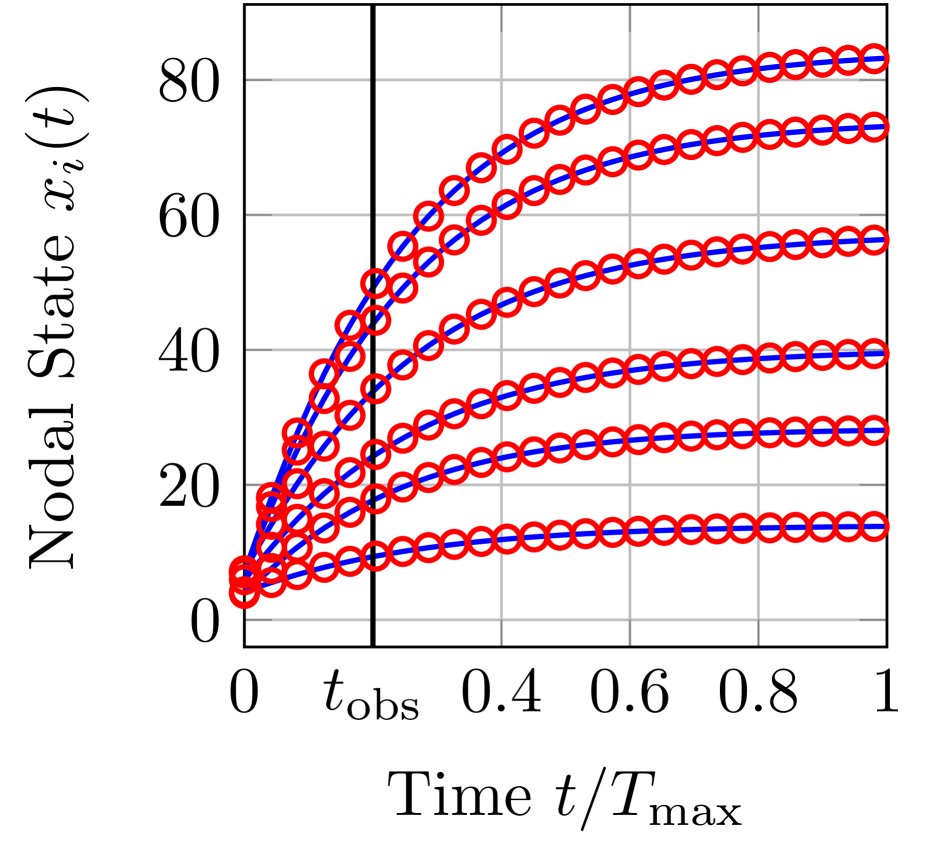
(f) CW ($N=282$)

Figure 4: Proper Orthogonal Decomposition of the Nodal State Dynamics. The exact nodal state $x(t)$ in blue and the approximation (9) in red. For readability, only six nodal states $x_{i}(t)$ are depicted for each network. The approximation equals the linear combination of $m=15$ agitation modes $y_{1}$, …, $y_{m}$, which are computed by observing the nodal state $x(t)$ from time $t=0$ to $t=t_{\textrm{obs}}$.

The Kuramoto oscillators are the only dynamics in Figure 2 that do not converge to a steady state $x_{\infty}$. Hence, the proper orthogonal decomposition (9) is not accurate when $t>>t_{\textrm{obs}}$, which explains that the prediction is least accurate for the Kuramoto model.

Why, precisely, is it not possible to reconstruct the network $A$? The linear system (3) forms the basis for the network reconstruction. The rank of the matrix $F_{i}$ is essential: If the matrix $F_{i}$ is of full rank, i.e., $\operatorname{rank}(F_{i})=N$, then there is exactly one solution to (3), namely the entries $a_{i1},...,a_{1N}$ of the true adjacency matrix $A$. Otherwise, if $\operatorname{rank}(F_{i})<N$, then there are infinitely many solutions to (3). If there is more than one solution to (3), then the LASSO estimation (6) results in the sparsest solution $\hat{A}$ (with respect to the $\ell_{1}$-norm).

We compute the numerical rank for Barabási-Albert random graphs versus the network size $N$. Here, we consider the best case for the network reconstruction: The derivative $dx_{i}(t)/dt$ is observed exactly, without any approximation error as in (2). Hence, the system (3) is satisfied with equality. Figure 5 shows that the numerical rank of the matrix $F_{i}$ stagnates as the network size $N$ grows. Hence, the linear system (3) is severely ill-conditioned for large networks. For example, for the SIS process on a network with $N=1000$ nodes, we observe a $1000\times 1001$ nodal state sequence $x(0)$, …, $x(1000\Delta t)$, but the numerical rank does not exceed $32$.

The matrix $F_{i}$, defined by (5), follows from applying the nonlinear function $g$ to the nodal state $x(t)$. The rank of the matrix $F_{i}$ is low, because the nodal state $x(t)$ is barely agitated, see Appendix C.

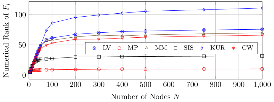
Figure 5: Ill-Condition of the Network Reconstruction. The numerical rank of the matrix $F_{i}$ of the linear system (3) versus the number of nodes $N$ for Barabási-Albert random graphs. The observation time is set to $t_{\textrm{obs}}=T_{\textrm{max}}$, and the number of observations equals $n=1000$.

6 Conclusions and Outlook

This works considers the prediction of general dynamics on networks, based on past observations of the dynamics. We proposed a prediction framework which consists of two steps. First, the network is estimated from the nodal state observations by the LASSO. The first step seemingly fails, since the estimated network bears no topological similarity with the true network. Second, the nodal state is predicted by iterating the dynamical model on the inaccurately estimated network. Counterintuitively, the prediction is accurate!

The network reconstruction and prediction accuracy do not match, because the nodal state is barely agitated. Furthermore, the modes of agitation are hardly related to the network topology. Instead of the true topology, the estimated network does capture the interplay with the agitation modes.

We conclude with five points. First, the agitation modes depend on the initial nodal dynamics and, particularly, on the initial nodal state $x(0)$. As a result, the estimated network $\hat{A}$ depends on the initial state $x(0)$. Thus, as confirmed by numerical simulations, the adjacency matrix $\hat{A}$ may be useless for the prediction of dynamics with a different initial state $\tilde{x}(0)\neq x(0)$.

Second, the dynamics (1) are autonomous, since there is no control input. In some applications [40, 26], it may be possible to control the nodal state $x(t)$. Controlling the dynamics would result in more agitation modes of the nodal state $x(t)$. However, physical control constraints, such as power capacities, might limit the number of additional agitation modes.

Third, we could observe multiple nodal state sequences $x(0),...,x(n\Delta)$ with different initial states  $x(0)$ on the same network. For sufficiently many sequences, we would observe enough agitation modes to reconstruct the network exactly, by stacking the respective linear systems (3). However, Figure 5 shows that the numerical rank of the matrix $F_{i}$ stagnates for large networks. Thus, the greater the network, the more time series must be observed to reconstruct the adjacency matrix $A$. Observing a sufficiently great number of time series might not be viable, e.g., for the epidemic outbreak of a novel virus like SARS-CoV-2.

Fourth, the proper orthogonal decomposition (7) can be exact. If the network has equitable partitions, then the number of agitation modes equals the number of cells for some dynamical models [41, 42, 43, 44, 45]. Furthermore, the SIS contagion dynamics reduce to only $m=1$ agitation mode around the epidemic threshold [46].

Fifth, the dynamics on two different networks $\hat{A}\neq A$ is exactly the same only if the networks satisfy (8). Based on numerical simulations, we showed that (8) holds approximately because the nodal state is barely agitated. We believe that the combination of the proper orthogonal decomposition (9) and equation (8) is a starting point for a further theoretical analysis on relating network structure and dynamics.

Appendix A Network Reconstruction Algorithm: Details and Bayesian Interpretation

Subsection A.1 states the reconstruction algorithm, which is an adaptation of the method we proposed in [26] for discrete-time epidemic models. The interpretation of the LASSO (6) as a Bayesian estimation problem is given in Subsection A.2.

A.1 Details of the Network Reconstruction Algorithm

The solution $\hat{a}_{i1}(\rho_{i}),...,\hat{a}_{iN}(\rho_{i})$ to the LASSO (6) depends on the regularisation parameter $\rho_{i}$. We aim to choose the parameter $\rho_{i}$ that results in the solution $\hat{a}_{i1}(\rho_{i}),...,\hat{a}_{iN}(\rho_{i})$ with the greatest prediction accuracy. To assess the prediction accuracy, we apply hold-out cross-validation [27]: We divide the nodal state observations into a training set $x(0),...,x(n_{\textrm{train}}\Delta t)$ and a validation set $x((n_{\textrm{train}}+1)\Delta t),...,x(n\Delta t)$. The training set is used to obtain the solution $\hat{a}_{i1}(\rho_{i}),...,\hat{a}_{iN}(\rho_{i})$ in dependency of $\rho_{i}$, whose prediction accuracy is evaluated on the validation set. We choose the regularisation parameter $\rho_{i}$ with the greatest prediction accuracy on the validation set.

More precisely, we define the training set as the first $80\%$ of the nodal state observations $x(0)$, $x(\Delta t)$, …, $x(n_{\textrm{train}}\Delta t)$, where $n_{\textrm{train}}=\lceil 0.8n\rceil$. We denote the $n_{\textrm{train}}\times 1$ training vector $V_{\textrm{train},i}$ as

$$V_{\textrm{train},i}=\begin{pmatrix}\dfrac{x_{i}\left(\Delta t\right)-x_{i}\left(0\right)}{\Delta t}-f_{i}(0)\\ \vdots\\ \dfrac{x_{i}\left(n_{\textrm{train}}\Delta t\right)-x_{i}\left(\left(n_{\textrm{train}}-1\right)\Delta t\right)}{\Delta t}-f_{i}\left(\left(n_{\textrm{train}}-1\right)\Delta t\right)\end{pmatrix}$$

and the $n_{\textrm{train}}\times N$ training matrix $F_{\textrm{train},i}$ as

$$F_{\textrm{train},i}=\\ \begin{pmatrix}g(x_{i}(0),x_{1}(0))&...&g(x_{i}(0),x_{N}(0))\\ \vdots&\ddots&\vdots\\ g\left(x_{i}\left(\left(n_{\textrm{train}}-1\right)\Delta t\right),x_{1}\left(\left(n_{\textrm{train}}-1\right)\Delta t\right)\right)&...&g\left(x_{i}\left(\left(n_{\textrm{train}}-1\right)\Delta t\right),x_{N}\left(\left(n_{\textrm{train}}-1\right)\Delta t\right)\right)\end{pmatrix}.$$

We denote the solution of the LASSO (6) by $\hat{a}_{i1}(\rho_{i}),...,\hat{a}_{iN}(\rho_{i})$, when $F_{i}$ and $V_{i}$ are replaced by $F_{\textrm{train},i}$ and $V_{\textrm{train},i}$, respectively. If an entry $\hat{a}_{ij}(\rho_{i})$ of the LASSO solution is smaller than the threshold $0.01$, then we round off and set $\hat{a}_{ij}(\rho_{i})=0$. The prediction error $\operatorname{MSE}(\rho_{i})$ of $\rho_{i}$ on the validation set is defined as

$$\operatorname{MSE}(\rho_{i})=\left\lVert V_{\textrm{valid},i}-F_{\textrm{valid},i}\begin{pmatrix}\hat{a}_{i1}(\rho_{i})\\ \vdots\\ \hat{a}_{iN}(\rho_{i})\end{pmatrix}\right\rVert^{2}_{2}.$$ (10)

Here, the $(n-n_{\textrm{train}})\times 1$ validation vector $V_{\textrm{valid},i}$ and the $(n-n_{\textrm{train}})\times N$ validation matrix $F_{\textrm{valid},i}$ are defined by the nodal state observations $x((n_{\textrm{train}}+1)\Delta t),...,x(n\Delta t)$, analogously to the training vector $V_{\textrm{train},i}$ and the training matrix $F_{\textrm{train},i}$

We iterate over a set $\Theta_{i}$, specified below, of predefined candidate values for $\rho_{i}$. Every candidate value $\rho_{i}\in\Theta_{i}$ results in a different prediction error $\operatorname{MSE}(\rho_{i})$. We determine the final regularisation parameter $\rho_{\textrm{opt},i}$ as the candidate value $\rho_{\textrm{opt},i}\in\Theta_{i}$ with the minimal prediction error $\operatorname{MSE}(\rho_{\textrm{opt},i})$. We obtain the final estimate $\hat{a}_{i1},...,\hat{a}_{iN}$ as the solution to the LASSO (6) with the regularisation parameter $\rho_{\textrm{opt},i}$, using the matrix $F_{i}$ and vector $V_{i}$ from all nodal state observations $x(0),...,x(n\Delta t)$.

We define the set $\Theta_{i}$ as 20 logarithmically equidistant candidate values as $\Theta_{i}=\{\rho_{\textrm{min},i},...,\rho_{\textrm{max},i}\}$. If $\rho_{i}>\rho_{\textrm{th},i}$, where $\rho_{\textrm{th},i}=2\lVert F^{T}_{i}V_{i}\rVert_{\infty}$, then [47] the solution to the LASSO (6) equals $a_{ij}=0$ for all nodes $j$. Thus, we set the candidate values in the set $\Theta_{i}$ proportional to $\rho_{\textrm{th},i}$. We define $\rho_{\textrm{min},i}=2\lVert F^{T}_{i}V_{i}\rVert_{\infty}10^{-6}$ and $\rho_{\textrm{max},i}=2\lVert F^{T}_{i}V_{i}\rVert_{\infty}10^{-2}$. The network reconstruction method is given by Algorithm 1.

Algorithm 1 Network reconstruction

1:Input: nodal state time series $x(0),x(\Delta t),...,x(n\Delta t)$

2:Output: estimated adjacency matrix $\hat{A}$ with the elements $\hat{a}_{ij}$

3:for $i=1,...,N$ do

4:     $\rho_{\textrm{max},i}\leftarrow 2\lVert F^{T}_{i}V_{i}\rVert_{\infty}10^{-2}$

5:     $\rho_{\textrm{min},i}\leftarrow~{}10^{-4}\rho_{\textrm{max},i}$

6:     $\Theta_{i}\leftarrow$ 20 logarithmically equidistant values from $\rho_{\textrm{min},i}$ to $\rho_{\textrm{max},i}$

7:     for $\rho_{i}\in\Theta_{i}$ do

8:         $\hat{a}_{i1}(\rho_{i}),...,\hat{a}_{iN}(\rho_{i})\leftarrow$ solution to (6) on the training set $V_{\textrm{train},i}$ and $F_{\textrm{train},i}$

9:         $\hat{a}_{ij}(\rho_{i})\leftarrow 0$ for all $\hat{a}_{i1}(\rho_{i}),...,\hat{a}_{iN}(\rho_{i})$ smaller than $0.01$

10:         Compute $\operatorname{MSE}(\rho_{i})$ by (10) on the validation set $V_{\textrm{valid},i}$ and $F_{\textrm{valid},i}$

11:     end for

12:     $\rho_{\textrm{opt},i}\leftarrow\underset{\rho_{i}\in\Theta_{i}}{\operatorname{argmin}}\operatorname{MSE}\left(\rho_{i}\right)$

13:     $(\hat{a}_{i1},...,\hat{a}_{iN})\leftarrow$ the solution to (6) for $\rho_{i}=\rho_{\textrm{opt},i}$ on the whole data set $F_{i},V_{i}$

14:     $\hat{a}_{ij}\leftarrow 0$ for all $\hat{a}_{i1},...,\hat{a}_{iN}$ smaller than $0.01$

15:end for

A.2 Interpretation as a Bayesian Estimation

For every node $i$, we define the error $w_{i}(k\Delta t)$ of the first-order approximation (2) of the derivative $dx_{i}(t)/dt$ at time $t=k\Delta t$, such that

$$x_{i}\left((k+1)\Delta t\right)=x_{i}\left(k\Delta t\right)+\Delta t\left.\frac{dx_{i}(t)}{dt}\right|_{t=k\Delta t}+w_{i}(k\Delta t).$$ (11)

The approximation (11) can be regarded as a nonlinear system in discrete time $k$ with random model errors $w_{i}(k\Delta t)$, which forms the basis for the Bayesian interpretation of the LASSO (6). Furthermore, we rely on two assumptions.

Assumption 1.

For every node $i$ at every time $k$, the approximation error $w_{i}(k\Delta t)$ follows the normal distribution $\mathcal{N}\left(0,\sigma^{2}_{w}\right)$ with zero mean and variance $\sigma^{2}_{w}$. Furthermore, the approximation errors $w_{i}(k\Delta t)$ are stochastically independent and identically distributed at all times $k=1,...,n$ and for all nodes $i$.

The exact model error $w_{i}(k\Delta t)$ is difficult to analyse, since $w_{i}(k\Delta t)$ is determined by higher-order derivatives of the nodal state $x(t)$. In contrast, assuming that the model error $w_{i}(k\Delta t)$ follows a Gaussian distribution $\mathcal{N}\left(0,\sigma^{2}_{w}\right)$ allows for a simple analysis. Furthermore, Assumption 1 stems from the maximum entropy principle [48]: Given a set of constraints on a probability distribution (e.g., specified mean), assume the “least informative” distribution, i.e., the distribution with maximum entropy that satisfies those constraint. Among all distributions on $\mathbb{R}$ with zero mean and variance $\sigma^{2}_{w}$, the Gaussian distribution $\mathcal{N}\left(0,\sigma^{2}_{w}\right)$ has the maximum entropy [49].

Assumption 2.

The adjacency matrix $A$ with non-negative elements $a_{ij}\geq 0$ follows the prior distribution

$$\operatorname{Pr}\left[A\right]=\alpha\exp\left(-\sum^{N}_{i=1}\sum^{N}_{j=1}a_{ij}\right),$$ (12)

where the normalisation constant $\alpha$ is set such that

$$\int_{\mathbb{R}^{N\times N}_{\geq 0}}\operatorname{Pr}\left[A\right]dA=1.$$

Furthermore, the matrix $A$ and the initial nodal state $x(0)$ are stochastically independent.

Clearly, there are more suitable random graph models for real-world networks than the exponential degree distribution in Assumption 2. In particular, the degree distribution of many real-world networks follows a power-law [50]. However, the central result in this work is given by the juxtaposition of Figure 2 with Figure 3: It is not necessary to accurately reconstruct the degree distribution to predict the dynamics on a network. Thus, even with the potentially imprecise assumption on the degree distribution (12), it is possible to accurately predict the dynamics on the network.

Proposition 2 states the Bayesian interpretation of the LASSO (6). We emphasise that Proposition 2 is not novel and follows standard arguments in parameter estimation, see for instance [51]. Furthermore, Tibshirani elaborated on the Bayesian interpretation of the LASSO in the seminal paper [52]. Nevertheless, we believe that the presentation of Proposition 2, here in the context of network reconstruction, is valuable to the reader.

Proposition 2.

Suppose that Assumption 1 and Assumption 2 hold true and that the nodal state $x(t)$ follows (11). Then, provided the regularisation parameter equals $\rho_{i}=2\sigma^{2}_{w}/\Delta t^{2}$, the matrix $\hat{A}$, which is obtained by solving the LASSO (6) for every node $i$, coincides with the Bayesian estimate:

$$\hat{A}=~{}\underset{A}{\operatorname{argmax}}~{}\operatorname{Pr}\left[A\big{|}x(0),...,x(n\Delta t)\right].$$ (13)

Proof.

Analogous steps to the derivations in [53] yield that (13) is equivalent to

$$\hat{A}=~{}\underset{A}{\operatorname{argmax}}~{}\log\left(\operatorname{Pr}\left[A\right]\right)+\sum^{n-1}_{k=0}\log\left(\operatorname{Pr}\left[x((k+1)\Delta t)\big{|}x(k\Delta t),A\right]\right).$$

Under Assumption 1, the errors $w_{i}(k\Delta t)$ are independent for different nodes $i$. Thus, we obtain that

$$\hat{A}=~{}\underset{A}{\operatorname{argmax}}~{}\log\left(\operatorname{Pr}\left[A\right]\right)+\sum^{n-1}_{k=0}\sum^{N}_{i=1}\log\left(\operatorname{Pr}\left[x_{i}((k+1)\Delta t)\big{|}x(k\Delta t),A\right]\right).$$ (14)

The probability $\operatorname{Pr}\left[x_{i}((k+1)\Delta t)\big{|}x(k\Delta t),A\right]$ is determined by the distribution of the error $w_{i}(k\Delta t)$. From (1) and (11), it follows that

$$w_{i}(k\Delta t)=x_{i}((k+1)\Delta t)-x_{i}(k\Delta t)-\Delta t\left(f_{i}\left(x_{i}(k\Delta t)\right)+\sum^{N}_{j=1}a_{ij}g\left(x_{i}(k\Delta t),x_{j}(k\Delta t)\right)\right).$$

With the definition of the vector $V_{i}$ and the matrix $F_{i}$ in (4) and (5), respectively, we obtain that

$$w_{i}((k-1)\Delta t)=\Delta t\left(V_{i}\right)_{k}-\Delta t\sum^{N}_{j=1}\left(F_{i}\right)_{kj}a_{ij}.$$

Hence, under Assumption 2 on the prior $\operatorname{Pr}\left[A\right]$, the optimisation problem (14) becomes

$$\begin{aligned} \hat{A}=~{}&\underset{A}{\operatorname{argmax}}~{}&&\log\left(\alpha\right)-\sum^{N}_{i=1}\sum^{N}_{j=1}a_{ij}&\\ &&&+\sum^{N}_{i=1}\sum^{n}_{k=1}\log\left(\operatorname{Pr}\left[w_{i}((k-1)\Delta t)=\Delta t\left(V_{i}\right)_{k}-\Delta t\sum^{N}_{j=1}\left(F_{i}\right)_{kj}a_{ij}\right]\right)&\\ &\text{s.t.}&&a_{ij}\geq 0\quad i,j=1,...,N.&\end{aligned}$$

The term $\log\left(\alpha\right)$ is constant with respect to the matrix $A$ and can be omitted. Furthermore, the optimisation can be carried out independently for every node $i$, which yields that

$$\begin{aligned} &\underset{a_{i1},...,a_{iN}}{\operatorname{max}}~{}&&\sum^{n}_{k=1}\log\left(\operatorname{Pr}\left[w_{i}((k-1)\Delta t)=\Delta t\left(V_{i}\right)_{k}-\Delta t\sum^{N}_{j=1}\left(F_{i}\right)_{kj}a_{ij}\right]\right)-\sum^{N}_{j=1}a_{ij}&\\ &\text{s.t.}&&a_{ij}\geq 0\quad j=1,...,N.&\end{aligned}$$

Under Assumption 1, the errors $w_{i}(k\Delta t)$ follow a Gaussian distribution, which results in the minimisation problem

$$\begin{aligned} &\underset{a_{i1},...,a_{iN}}{\operatorname{min}}~{}&&\sum^{n}_{k=1}\log(\sqrt{2\pi}\sigma_{w})+\frac{1}{2\sigma^{2}_{w}}\left(\Delta t\left(V_{i}\right)_{k}-\Delta t\sum^{N}_{j=1}\left(F_{i}\right)_{kj}a_{ij}\right)^{2}+\sum^{N}_{j=1}a_{ij}&\\ &\text{s.t.}&&a_{ij}\geq 0\quad j=1,...,N.&\end{aligned}$$

Omitting the constant term $\log(\sqrt{2\pi}\sigma_{w})$ and multiplying with $2\sigma^{2}_{w}/\Delta t^{2}$ gives

$$\begin{aligned} &\underset{a_{i1},...,a_{iN}}{\operatorname{min}}~{}&&\sum^{n}_{k=1}\left(\left(V_{i}\right)_{k}-\sum^{N}_{j=1}\left(F_{i}\right)_{kj}a_{ij}\right)^{2}+2\frac{\sigma^{2}_{w}}{\Delta t^{2}}\sum^{N}_{j=1}a_{ij}&\\ &\text{s.t.}&&a_{ij}\geq 0\quad j=1,...,N.&\end{aligned}$$

By identifying $\rho_{i}=2\sigma^{2}_{w}/\Delta t^{2}$, we obtain the LASSO (6), which completes the proof. ∎

Appendix B Details on the Empirical Networks and Model Parameters

Here, we provide details on the empirical networks and the parameters for the respective network dynamics in Section 2. For every network topology, we obtain the link weights $a_{ij}$ as follows. If there is a link from node $j$ to node $i$, then we set the element $a_{ij}$ to a uniformly distributed random number in $[0.5,1.5]$. If there is no link from node $j$ to node $i$, then we set the respective element to $a_{ij}=0$.

B.1 Lotka-Volterra Population Dynamics

For the competitive population dynamics described by the Lotka-Volterra equations, we consider the Little Rock Lake network [28], which we accessed via the Konect network collection [54]. The asymmetric and connected network consists of $N=183$ nodes, which correspond to different species. There are $L=2494$ directed links which specify the predation of one species upon another.

For every species $i$, we set the growth parameters $\alpha_{i}$ and $\theta_{i}$ to uniformly distributed random numbers in $[0.5,1.5]$. Furthermore, we set the the initial nodal state $x_{i}(0)$ to a uniformly distributed random number in $[0,1]$ for every species $i$. We set the maximum prediction time to $T_{\textrm{max}}=5$.

B.2 Mutualistic Population Dynamics

Kato et al. [29] studied the relationship between $679$ insect species and $91$ plants in a beech forest in Kyoto by specifying which insects pollinate or disperse which plant. We accessed the insect-plant network via the supplementary data in [30]. The insect-plant network determines a mutualistic insect-insect network [15]: If two insect species $i$ and $j$ pollinate or disperse the same plant, then both insect species $i$ and $j$ contribute to, and benefit from, the abundance of the plant. Thus, if two insect species $i$ and $j$ are linked to the same plant, then we set $a_{ij}$ to a uniformly distributed random number in $[0.5,1.5]$, and $a_{ij}=0$ otherwise. As a result, we obtain a symmetric and disconnected network with $N=679$ nodes and $L=30,905$ links.

For every species $i$, we set the growth parameters $\alpha_{i}$ and $\theta_{i}$ to a uniformly distributed random number in $[0.5,1.5]$. Furthermore, we set the the initial nodal state $x_{i}(0)$ to a uniformly distributed random number in $[0,20]$ for every species $i$. We set the maximum prediction time to $T_{\textrm{max}}=0.025$.

B.3 Michaelis-Menten Regulatory Dynamics

We consider the transcription interactions between regulatory genes in the yeast S. Cerevisiae [31]. The asymmetric and disconnected network has $N=620$ and $L=869$ links. The influence from gene $j$ to gene $i$ is in either an activation or inhibition regulation. Since the activator interactions account for more than $80\%$ of the links between genes, we only consider activation interactions, see also [12]. In line with Harush and Barzel [15], we consider degree avert regulatory dynamics by setting the Hill coefficient to $h=2$. We set the the initial nodal state $x_{i}(0)$ to a uniformly distributed random number in $[0,2]$ for every node $i$. We set the maximum prediction time to $T_{\textrm{max}}=3$.

B.4 Susceptible-Infected-Susceptible Epidemics

The SIS contagion dynamics are evaluated on the contact network of the Infectious: Stay Away exhibition [32] between $N=410$ individuals, accessed via [54]. The connected and symmetric network has $L=5530$ links. A link between two nodes $i$,$j$ indicates that the respective two individuals had a face-to-face contact that lasted for at least 20 seconds.

A crucial quantity for the SIS dynamics is the basic reproduction number $R_{0}$, which is defined as [55]

$$R_{0}=\rho\left(\operatorname{diag}\left(\delta_{1},...,\delta_{N}\right)^{-1}B\right).$$ (15)

Here, the spectral radius of an $N\times N$ matrix $M$ is denoted by $\rho(M)$, and $\operatorname{diag}\left(\delta_{1},...,\delta_{N}\right)$ denotes the $N\times N$ diagonal matrix with the curing rates $\delta_{1},...,\delta_{N}$ on its diagonal. If the basic reproduction number $R_{0}$ is less than or equal to 1, then the epidemic dies out [19], i.e., $x(t)\rightarrow 0$ as $t\rightarrow\infty$. We would like to study the spread of a virus that does not die out, and we aim to set the basic reproduction number to $R_{0}=1.5$: First, we set the “initial curing rate” $\delta^{(0)}_{i}$ to a uniformly distributed random number in $[0.5,1.5]$ for every node $i$. Then, we set the curing rates to $\delta_{i}=c\delta^{(0)}_{i}$, where the multiplicity $c$ is chosen such that the basic reproduction number in (15) equals $R_{0}=1.5$. We set the the initial nodal state $x_{i}(0)$ to a uniformly distributed random number in $[0,0.1]$ for every node $i$. Furthermore, we set the maximum prediction time to $T_{\textrm{max}}=0.5$.

B.5 Kuramoto Oscillators

We consider Kuramoto oscillator dynamics on the structural human brain network [56] of size $N=78$. Every node corresponds to a brain region of the automated anatomical labelling (AAL) atlas [57]. The structural brain network specifies the anatomical connectivity between regions, i.e., the physical connections between regions based on white matter tracts. White matter tracts were estimated using fibre tracking from diffusion MRI data from the Human Connectome Project [33] as outlined in [34]. The network is symmetric and has $L=696$ links.

For every node $i$, we set the natural frequency $\omega_{i}$ to a normally distributed random number with zero mean and standard deviation $0.1\pi$. Furthermore, we set the the initial nodal state $x_{i}(0)$ to a uniformly distributed random number in $[-\pi/4,\pi/4]$ for every node $i$. We set the maximum prediction time to $T_{\textrm{max}}=1$.

B.6 Cowan-Wilson Neural Firing

We consider the modified Cowan-Wilson neural firing model of Laurence et al. [13] on the neuronal connectivity of the adult Caenorhabditis elegans hermaphrodite worm. Originally, White et al. [35] compiled the neuronal connectivity of C. elegans. In [36, 58], the neural wiring was updated, which we accessed online via the Wormatlas online database. The somatic nervous system has $N=282$ neurons and $L=2994$ synapses. A link from node $j$ to node $i$ indicates the presence of at least one synapse from neuron $j$ to neuron $i$.

The slope and the threshold of the neural activation functions are set to $\tau=1$ and $\mu=1$, respectively. The initial state $x_{i}(0)$ of every node $i$ is set to a uniformly distributed random number in $[0,10]$. We set the maximum prediction time to $T_{\textrm{max}}=4$.

Appendix C Ill-Conditioning of the Network Reconstruction

We argue that if the proper orthogonal decomposition (9) is accurate, then the matrix $F_{i}$ in (5) is ill-conditioned. We rewrite the matrix $F_{i}$ as

$$F_{i}=\begin{pmatrix}r^{T}_{i}(x\left(0\right))\\ \vdots\\ r^{T}_{i}(x\left((n-1)\Delta t\right))\end{pmatrix},$$

where the rows are given by $N\times 1$ vectors

$$r_{i}\left(x\left(k\Delta t\right)\right)=\begin{pmatrix}g\left(x_{i}\left(k\Delta t\right),x_{1}\left(k\Delta t\right)\right)\\ \vdots\\ g\left(x_{i}\left(k\Delta t\right),x_{N}\left(k\Delta t\right)\right)\end{pmatrix}.$$ (16)

We aim to show that the approximation of the nodal state $x(t)$ in (9) implies that the row vectors $r_{i}(x(k\Delta t))$, where $k=0,1,...,n-1$, can be approximated by the linear combination of only few vectors, which implies the ill-conditioning of the matrix $F_{i}$. To shorten the notation, we drop the time index $t$ in this section. More precisely, we formally replace the nodal state $x(t)$ by $x$ and the functions $g\left(x_{i}(t),x_{j}(t)\right)$ and $r_{i}(x(t))$ by $g\left(x_{i},x_{j}\right)$ and $r_{i}(x)$, respectively.

To analyse the nonlinear dependency of the rows $r_{i}(x)$ on the nodal state $x$, we resort to a Taylor expansion of the rows $r_{i}(x)$. The function $r_{i}:\mathbb{R}^{N}\rightarrow\mathbb{R}^{N}$ is specified by the nonlinear interaction function $g$ of the dynamical model (1). The Taylor expansion of the function $g(x_{i},x_{j})$ around the point $x_{i}=x_{j}=0$ reads

$$g\left(x_{i},x_{j}\right)=g(0,0)+\sum^{\infty}_{k=1}\sum_{\alpha+\beta=k}\frac{1}{\alpha!\beta!}x^{\alpha}_{i}x^{\beta}_{j}\left.\frac{\partial^{k}g\left(x_{i},x_{j}\right)}{\partial x^{\alpha}_{i}\partial x^{\beta}_{j}}\right|_{x_{i}=x_{j}=0}.$$ (17)

We define the coefficient $\eta\left(\alpha,\beta\right)$ as

$$\eta\left(\alpha,\beta\right)=\frac{1}{\alpha!\beta!}\left.\frac{\partial^{k}g\left(x_{i},x_{j}\right)}{\partial x^{\alpha}_{i}\partial x^{\beta}_{j}}\right|_{x_{i}=x_{j}=0}.$$ (18)

The indices $i$ and $j$ refer to the first and second argument of the function $g(x_{i},x_{j})$. Thus, the coefficient $\eta\left(\alpha,\beta\right)$ does not depend on the value of the indices $i$, $j$. With (18), it follows from (17) that

$$g\left(x_{i},x_{j}\right)=g(0,0)+\sum^{\infty}_{k=1}\sum^{k}_{\alpha=0}\eta\left(\alpha,k-\alpha\right)x^{\alpha}_{i}x^{k-\alpha}_{j}.$$ (19)

With (19), we obtain the Taylor series of the function $r_{i}$ in (16) as

$$r_{i}(x)=r_{i}(0)+\sum^{\infty}_{k=1}\sum^{k}_{\alpha=0}\eta\left(\alpha,k-\alpha\right)x^{\alpha}_{i}x^{k-\alpha},$$ (20)

where we denote the element-wise power of the vector $x$ as

$$x^{k-\alpha}=\left(x^{k-\alpha}_{1},...,x^{k-\alpha}_{N}\right)^{T}.$$

We define the truncation of the series (20) until the $q$-th power as

$$r_{q,i}\left(x\right)=r_{i}(0)+\sum^{q}_{k=1}\sum^{k}_{\alpha=0}\eta\left(\alpha,k-\alpha\right)x^{\alpha}_{i}x^{k-\alpha}.$$ (21)

For a sufficiently great power $q$, the matrix $F_{i}$ is approximated by $F_{i}\approx F_{q,i}$, where we define the matrix $F_{q,i}$ with the truncations $r_{q,i}(x)$ as

$$F_{q,i}=\begin{pmatrix}r^{T}_{q,i}(x\left(0\right))\\ \vdots\\ r^{T}_{q,i}(x\left((n-1)\Delta t\right))\end{pmatrix}.$$

In fact, if the interaction function $g(x_{i},x_{j})$ is a polynomial of degree $q$, then the matrices $F_{i}$ and $F_{q,i}$ coincide, i.e., $F_{i}=F_{q,i}$. For instance, it holds that $F_{i}=F_{2,i}$ for the SIS epidemic process whose interaction function equals $g(x_{i},x_{j})=(1-x_{i})x_{j}$. The low agitation of the nodal state vector $x$ in (9) indeed explains the ill-conditioning of the matrix $F_{i}$:

Proposition 3.

Suppose that the $N\times 1$ nodal state vector $x(t)$ equals the linear combination of $m$ vectors $y_{p}$ at every time $t$,

$$x(t)=\sum^{m}_{p=1}c_{p}(t)y_{p}$$ (22)

for some scalars $c_{p}(t)\in\mathbb{R}$. Then, the rank of the matrix $F_{q,i}$ is bounded by

$$\operatorname{rank}\left(F_{q,i}\right)\leq\sum^{q}_{\beta=0}{{\beta+m-1}\choose{m-1}}.$$

Proof.

It follows from (22) that

$$x(t)\in\operatorname{span}\left(y_{1},...,y_{m}\right)$$

at every time $t$, where $\operatorname{span}\left(y_{1},...,y_{m}\right)$ denotes the span of the vectors $y_{1}$, …, $y_{m}$. We rewrite the function $r_{q,i}\left(x\right)$ in (21) as

$$r_{q,i}\left(x\right)=r_{i}(0)+\sum^{q}_{k=1}\sum^{k}_{\beta=0}\eta\left(k-\beta,\beta\right)x^{k-\beta}_{i}x^{\beta}.$$

Both terms $\eta\left(k-\beta,\beta\right)$ and $x^{k-\beta}_{i}$ are scalars. Thus, we obtain that

$$r_{q,i}\left(x\right)=r_{i}(0)+\sum^{q}_{\beta=0}\mu_{\beta}(x)x^{\beta}$$ (23)

for some scalars $\mu_{0}(x),\mu_{1}(x),...,\mu_{q}(x)\in\mathbb{R}$. Since the rows of the matrix $F_{q,i}$ are given by (23) for some $x\in\operatorname{span}\left(y_{1},...,y_{m}\right)$, it holds that

$$\operatorname{rank}\left(F_{q,i}\right)\leq\sum^{q}_{\beta=0}\operatorname{dim}\left(\left\{x^{\beta}\big{|}x\in\operatorname{span}\left(y_{1},...,y_{m}\right)\right\}\right).$$ (24)

We consider the addends in (24) separately. For any vector $x\in\operatorname{span}\left(y_{1},...,y_{m}\right)$, it holds that

$$x^{\beta}_{j}=\left(\sum^{m}_{p=1}c_{p}\left(y_{p}\right)_{j}\right)^{\beta}$$

for some scalars $c_{1},...,c_{m}$. The multinomial theorem yields that

$$x^{\beta}_{j}=\sum_{p_{1}+p_{2}+...+p_{m}=\beta}\frac{\beta!}{p_{1}!p_{2}!\cdots p_{m}!}\prod^{m}_{l=1}\left(c_{l}\left(y_{l}\right)_{j}\right)^{p_{l}}.$$

We define the coefficients

$$\zeta\left(p_{1},...,p_{m}\right)=\frac{\beta!}{p_{1}!p_{2}!\cdots p_{m}!}\prod^{m}_{l=1}\left(c_{l}\right)^{p_{l}},$$

which gives that

$$x^{\beta}_{j}=\sum_{p_{1}+p_{2}+...+p_{m}=\beta}\zeta\left(p_{1},...,p_{m}\right)\prod^{m}_{l=1}\left(y_{l}\right)^{p_{l}}_{j}.$$ (25)

By stacking (25) for the entries $j=1,...,N$, we obtain an expression for the vector $x^{\beta}$ as

$$x^{\beta}=\sum_{p_{1}+p_{2}+...+p_{m}=\beta}\zeta\left(p_{1},...,p_{m}\right)\nu\left(p_{1},...,p_{m}\right).$$ (26)

Here, we defined the vectors

$$\nu\left(p_{1},...,p_{m}\right)=\left(y_{1}\right)^{p_{1}}\odot\left(y_{2}\right)^{p_{2}}\odot...\odot\left(y_{m}\right)^{p_{m}},$$

where $\odot$ denotes the Hadamard product, or element-wise product. From (26), it follows that the vector $x^{\beta}$ is a linear combination of all vectors $\nu\left(p_{1},...,p_{m}\right)$ with $p_{1}+p_{2}+...+p_{m}=\beta$, which yields that

$$\operatorname{dim}\left(\left\{x^{\beta}\big{|}x\in\operatorname{span}\left(y_{1},...,y_{m}\right)\right\}\right)={{\beta+m-1}\choose{m-1}}.$$ (27)

We complete the proof by combining (24) and (27). ∎

As an example, consider that the nodal state $x(t)$ of the SIS epidemic process is agitated in only $m=10$ agitation modes $y_{p}$. Then, since $F_{i}=F_{2,i}$ for the SIS epidemic process, Proposition 3 states that

$$\operatorname{rank}\left(F_{i}\right)=\operatorname{rank}\left(F_{2,i}\right)\leq\sum^{2}_{\beta=0}{{\beta+10-1}\choose{10-1}},$$

which yields that $\operatorname{rank}\left(F_{i}\right)\leq 66$.

References

- [1] R. May, Stability and complexity in model ecosystems. Princeton University Press, 2001, vol. 6.
- [2] R. Pastor-Satorras, C. Castellano, P. Van Mieghem, and A. Vespignani, “Epidemic processes in complex networks,” Reviews of Modern Physics, vol. 87, no. 3, pp. 925––979, 2015.
- [3] J. Cabral, M. L. Kringelbach, and G. Deco, “Exploring the network dynamics underlying brain activity during rest,” Progress in Neurobiology, vol. 114, pp. 102–131, 2014.
- [4] S. Boccaletti, V. Latora, Y. Moreno, M. Chavez, and D.-U. Hwang, “Complex networks: Structure and dynamics,” Physics Reports, vol. 424, no. 4-5, pp. 175–308, 2006.
- [5] A. Barrat, M. Barthelemy, and A. Vespignani, Dynamical processes on complex networks. Cambridge University Press, 2008.
- [6] M. A. Porter and J. P. Gleeson, “Dynamical systems on networks,” Frontiers in Applied Dynamical Systems: Reviews and Tutorials, vol. 4, 2016.
- [7] M. Timme and J. Casadiego, “Revealing networks from dynamics: an introduction,” Journal of Physics A: Mathematical and Theoretical, vol. 47, no. 34, p. 343001, 2014.
- [8] W.-X. Wang, Y.-C. Lai, and C. Grebogi, “Data based identification and prediction of nonlinear and complex dynamical systems,” Physics Reports, vol. 644, pp. 1–76, 2016.
- [9] M. Newman, “Network structure from rich but noisy data,” Nature Physics, vol. 14, no. 6, p. 542, 2018.
- [10] T. P. Peixoto, “Network reconstruction and community detection from dynamics,” Physical Review Letters, vol. 123, p. 128301, Sep 2019.
- [11] A. Barrat, M. Barthelemy, R. Pastor-Satorras, and A. Vespignani, “The architecture of complex weighted networks,” Proceedings of the National Academy of Sciences, vol. 101, no. 11, pp. 3747–3752, 2004.
- [12] B. Barzel and A.-L. Barabási, “Universality in network dynamics,” Nature Physics, vol. 9, no. 10, p. 673, 2013.
- [13] E. Laurence, N. Doyon, L. J. Dubé, and P. Desrosiers, “Spectral dimension reduction of complex dynamical networks,” Physical Review X, vol. 9, no. 1, p. 011042, 2019.
- [14] R. MacArthur, “Species packing and competitive equilibrium for many species,” Theoretical Population Biology, vol. 1, no. 1, pp. 1–11, 1970.
- [15] U. Harush and B. Barzel, “Dynamic patterns of information flow in complex networks,” Nature Communications, vol. 8, no. 1, p. 2181, 2017.
- [16] U. Alon, An introduction to systems biology: design principles of biological circuits. CRC Press, 2006.
- [17] J. Gao, B. Barzel, and A.-L. Barabási, “Universal resilience patterns in complex networks,” Nature, vol. 530, no. 7590, p. 307, 2016.
- [18] N. T. J. Bailey, The Mathematical Theory of Infectious Diseases and Its Applications. Charles Griffin & Company, London, 1975, no. 2nd edition.
- [19] A. Lajmanovich and J. A. Yorke, “A deterministic model for gonorrhea in a nonhomogeneous population,” Mathematical Biosciences, vol. 28, no. 3-4, pp. 221–236, 1976.
- [20] P. Van Mieghem, J. Omic, and R. Kooij, “Virus spread in networks,” IEEE/ACM Transactions on Networking, vol. 17, no. 1, pp. 1–14, 2009.
- [21] Y. Kuramoto, Chemical oscillations, waves, and turbulence. Courier Corporation, 2003.
- [22] H. R. Wilson and J. D. Cowan, “Excitatory and inhibitory interactions in localized populations of model neurons,” Biophysical Journal, vol. 12, no. 1, pp. 1–24, 1972.
- [23] S. H. Strogatz, “Exploring complex networks,” Nature, vol. 410, no. 6825, pp. 268–276, 2001.
- [24] T. Hastie, R. Tibshirani, and M. Wainwright, Statistical learning with sparsity: the lasso and generalizations. CRC press, 2015.
- [25] Z. Shen, W.-X. Wang, Y. Fan, Z. Di, and Y.-C. Lai, “Reconstructing propagation networks with natural diversity and identifying hidden sources,” Nature Communications, vol. 5, pp. 1–10, 2014.
- [26] B. Prasse and P. Van Mieghem, “Network reconstruction and prediction of epidemic outbreaks for general group-based compartmental epidemic models,” IEEE Transactions on Network Science and Engineering, 2020.
- [27] C. Bergmeir and J. M. Benítez, “On the use of cross-validation for time series predictor evaluation,” Information Sciences, vol. 191, pp. 192–213, 2012.
- [28] N. D. Martinez, “Artifacts or attributes? Effects of resolution on the Little Rock Lake food web,” Ecological Monographs, vol. 61, no. 4, pp. 367–392, 1991.
- [29] M. Kato, T. Kakutani, T. Inoue, and T. Itino, “Insect-flower relationship in the primary beech forest of Ashu, Kyoto: an overview of the flowering phenology and the seasonal pattern of insect visits,” Contributions from the Biological Laboratory Kyoto University, vol. 27, pp. 309–375, 1990.
- [30] E. L. Rezende, J. E. Lavabre, P. R. Guimarães, P. Jordano, and J. Bascompte, “Non-random coextinctions in phylogenetically structured mutualistic networks,” Nature, vol. 448, no. 7156, p. 925, 2007.
- [31] R. Milo, S. Shen-Orr, S. Itzkovitz, N. Kashtan, D. Chklovskii, and U. Alon, “Network motifs: simple building blocks of complex networks,” Science, vol. 298, no. 5594, pp. 824–827, 2002.
- [32] L. Isella, J. Stehlé, A. Barrat, C. Cattuto, J.-F. Pinton, and W. Van den Broeck, “What’s in a crowd? Analysis of face-to-face behavioral networks,” Journal of Theoretical Biology, vol. 271, no. 1, pp. 166–180, 2011.
- [33] D. C. Van Essen, S. M. Smith, D. M. Barch, T. E. J. Behrens, E. Yacoub, and K. Ugurbil, “The WU-Minn Human Connectome Project: an overview,” NeuroImage, vol. 80, pp. 62–79, 2013.
- [34] P. Tewarie, R. Abeysuriya, Á. Byrne, G. C. O’Neill, S. N. Sotiropoulos, M. J. Brookes, and S. Coombes, “How do spatially distinct frequency specific MEG networks emerge from one underlying structural connectome? The role of the structural eigenmodes,” NeuroImage, vol. 186, pp. 211–220, 2019.
- [35] J. G. White, E. Southgate, J. N. Thomson, and S. Brenner, “The structure of the nervous system of the nematode Caenorhabditis elegans,” Philos. Trans. Roy. Soc. London, vol. 314, no. 1165, pp. 1–340, 1986.
- [36] B. L. Chen, D. H. Hall, and D. B. Chklovskii, “Wiring optimization can relate neuronal structure and function,” Proceedings of the National Academy of Sciences, vol. 103, no. 12, pp. 4723–4728, 2006.
- [37] T. Fawcett, “An introduction to ROC analysis,” Pattern Recognition Letters, vol. 27, no. 8, pp. 861–874, 2006.
- [38] A. C. Antoulas, Approximation of large-scale dynamical systems. SIAM, 2005, vol. 6.
- [39] G. Kerschen, J.-c. Golinval, A. F. Vakakis, and L. A. Bergman, “The method of proper orthogonal decomposition for dynamical characterization and order reduction of mechanical systems: an overview,” Nonlinear Dynamics, vol. 41, no. 1-3, pp. 147–169, 2005.
- [40] M. Timme, “Revealing network connectivity from response dynamics,” Physical review letters, vol. 98, no. 22, p. 224101, 2007.
- [41] P. Van Mieghem, Graph spectra for complex networks. Cambridge University Press, 2010.
- [42] N. O’Clery, Y. Yuan, G.-B. Stan, and M. Barahona, “Observability and coarse graining of consensus dynamics through the external equitable partition,” Physical Review E, vol. 88, no. 4, p. 042805, 2013.
- [43] S. Bonaccorsi, S. Ottaviano, D. Mugnolo, and F. D. Pellegrini, “Epidemic outbreaks in networks with equitable or almost-equitable partitions,” SIAM Journal on Applied Mathematics, vol. 75, no. 6, pp. 2421–2443, 2015.
- [44] M. T. Schaub, N. O’Clery, Y. N. Billeh, J.-C. Delvenne, R. Lambiotte, and M. Barahona, “Graph partitions and cluster synchronization in networks of oscillators,” Chaos: An Interdisciplinary Journal of Nonlinear Science, vol. 26, no. 9, p. 094821, 2016.
- [45] K. Devriendt and R. Lambiotte, “Non-linear network dynamics with consensus-dissensus bifurcation,” arXiv preprint arXiv:2002.08408, 2020.
- [46] B. Prasse and P. Van Mieghem, “Time-dependent solution of the NIMFA equations around the epidemic threshold,” Submitted, 2019.
- [47] S.-J. Kim, K. Koh, M. Lustig, S. Boyd, and D. Gorinevsky, “An interior-point method for large-scale -regularized least squares,” IEEE Journal of Selected Topics in Signal Processing, vol. 1, no. 4, pp. 606–617, 2007.
- [48] E. T. Jaynes, “Information theory and statistical mechanics,” Physical Review, vol. 106, no. 4, p. 620, 1957.
- [49] A. Papoulis and S. U. Pillai, Probability, random variables, and stochastic processes. Tata McGraw-Hill Education, 2002.
- [50] A.-L. Barabási, Network Science. Cambridge University Press, 2016.
- [51] R. C. Aster, B. Borchers, and C. H. Thurber, Parameter estimation and inverse problems. Elsevier, 2018.
- [52] R. Tibshirani, “Regression shrinkage and selection via the lasso,” Journal of the Royal Statistical Society. Series B (Methodological), pp. 267–288, 1996.
- [53] B. Prasse and P. Van Mieghem, “Exact network reconstruction from complete SIS nodal state infection information seems infeasible,” IEEE Transactions on Network Science and Engineering, vol. 6, no. 4, pp. 748–759, 2018.
- [54] J. Kunegis, “Konect: the Koblenz network collection,” in Proceedings of the 22nd International Conference on World Wide Web. ACM, 2013, pp. 1343–1350.
- [55] P. Van den Driessche and J. Watmough, “Reproduction numbers and sub-threshold endemic equilibria for compartmental models of disease transmission,” Mathematical Biosciences, vol. 180, no. 1-2, pp. 29–48, 2002.
- [56] M. Breakspear, S. Heitmann, and A. Daffertshofer, “Generative models of cortical oscillations: neurobiological implications of the Kuramoto model,” Frontiers in Human Neuroscience, vol. 4, p. 190, 2010.
- [57] N. Tzourio-Mazoyer, B. Landeau, D. Papathanassiou, F. Crivello, O. Etard, N. Delcroix, B. Mazoyer, and M. Joliot, “Automated anatomical labeling of activations in SPM using a macroscopic anatomical parcellation of the MNI MRI single-subject brain,” NeuroImage, vol. 15, no. 1, pp. 273–289, 2002.
- [58] L. R. Varshney, B. L. Chen, E. Paniagua, D. H. Hall, and D. B. Chklovskii, “Structural properties of the Caenorhabditis elegans neuronal network,” PLoS Computational Biology, vol. 7, no. 2, 2011.