Identifying Dark Matter Haloes by the Caustic Boundary

Abstract

Dark matter density is formally infinite at the location of caustic surfaces, where dark matter sheet folds in phase space. The caustics separate multi-stream regions with different number of streams. Volume elements change the parity by turning inside out when passing through the caustic stage. Being measure-zero structures, identification of caustics via matter density fields is usually restricted to fine-grained simulations. Instead a generic purely geometric algorithm can be employed to identify caustics directly by using triangulation of Lagrangian sub-manifold ${\bf x}({\bf q},t)$ where ${\bf x}$ and ${\bf q}$ are Eulerian and Lagrangian coordinates obtained in N-body simulations. The caustic surfaces are approximated by a set of triangles with vertices being the particles in the simulation. It is demonstrated that finding a dark matter halo is quite feasible by building its outermost convex caustic. Neither more specific assumptions about the geometry of the boundary nor ad hoc parameters are needed. The halo boundary in our idealized but undoubtably generic simulation is neither spherical nor ellipsoidal but rather remarkably asymmetrical. The analysis of the kinetic and potential energies of individual particles and the halo as a whole along with an examination of the two-dimensional phase space has shown that the halo is gravitationally bound.

1 Introduction

Caustics along with the multi-stream regions and flip-flop field are inherent features of the cold collision-less dark matter (DM) web. Known in geometric optics as an envelope of light rays reflected or refracted by a smooth curved surface a caustic is a line or point where the light intensity approaches infinity when the wavelength of the illuminating light tends to zero. The Zeldovich Approximation (ZA) [1] in two-dimensional space is identical to refraction of parallel light rays by a plate with thickness given by a two-dimensional random smooth function. When a screen is placed behind the plate then bright caustic patterns can be observed in a certain range of distances from the plate. These patterns are exactly the same as the web structures predicted by the ZA in two-dimensional case [2, 3]. The intensity of light in caustic is high but finite since the wave nature of light. Similarly the density in caustics in a cold collision-less DM is high but finite because of two reasons. First, DM is not a continuous medium and second – more importantly – because a finite thermal velocity dispersion. However, the smaller the velocity dispersion the higher density in the caustics, see e.g. [4]. Nevertheless the approximation of DM by a cold continuous medium is extremely accurate and commonly used in cosmology.

Along with the caustics the CDM web possesses two additional traits that cannot be found in a collisional medium like baryonic component in the universe. They are multi-stream flows and flip-flops of fluid particles. All three closely connected but not identical phenomena. They can be used as additional quantitative characteristics of the DM web. The multi-stream field is simply a count of the streams with distinct velocities at every point in Eulerian space. Generally the number of streams is an odd integer except the caustic surfaces where it is an even integer. The flip-flop field is the count of turns inside out for each fluid element. Both can be evaluated in cosmological N-body simulations. It can be done either on particles or tetrahedra of the tessellation of the three-dimensional phase space sheet in six dimensional phase space [5, 6]. The tessellation technique allows to considerably improve N-body simulations [7, 8, 9] and provides additional effective diagnostics for the analysis of the complexity of the DM web [10, 11, 12, 13, 14].

The multi-stream field in N-body simulations is naturally to evaluate on arbitrary set of diagnostic points in Eulerian space [15, 5, 16]. On the other hand the flip-flop field can be easily computed on particles or tetrahedra in Lagrangian space [10, 14]. Of course the flip-flop field can be mapped to Eulerian space but this would significantly change its mathematical properties – being a field in Lagrangian space – it becomes a multi-valued function in Eulerian space which is more difficult to deal with. Caustics are the interfaces between regions with different values of flip-flops in Lagrangian space and between regions with different values of the number of streams in Eulerian space.

In principle caustics surfaces can be identified as very thin layers of very high DM densities but it would require N-body simulations with unfeasibly high mass resolution for realistic cosmological simulations. However, since caustics separate the Lagrangian neighbor elements with different number of flip-flops it is also possible to use the common faces of two neighboring tetrahedra with opposite parities as a natural representation of the elements of caustic surfaces [5, 6].

Topological analysis and classification of all generic types of caustics originating in a potential mapping of a collision-less medium in two and three dimensions were provided in [17]. However, the analysis was based on the so called normal forms which roughly speaking are the minimal polynomials used as generators of singularities. In this form the results can be used only as a solid guideline for the much more strenuous analysis of realistic DM flows in cosmological simulations. The first analysis of the geometry and topology of the caustic structures in the frame of the ZA with smooth random initial perturbations was done in [18], however, it was limited to two dimensions.

For the recent scrutiny of the subject see [19] and [20]. However, the authors of [19] showed the 3D caustics only in the ZA simulation and the authors of [20] showed bicaustics (according to Arnold’s terminology) in 3D N-body simulations but not the caustics themselves. In simple terms, a bicaustic is the trace of an instantaneous caustic moving with time. In this paper we focus on A2 caustics which are surfaces at each instant of time after emergence at the nonlinear stage.

The presence of caustics has been implied in most if not all modern cosmological N-body simulations. For example, a splashback radius defined in [21, 22] as the distance from the center of a halo to its outermost closed caustic in the spherical models. The authors argued that the splashback radius is a more physical choice of the halo’s boundary than one based on a density contrast $\Delta$ relative to a reference density (mean or critical). However, they did not identify caustics directly. Instead they searched for a minimum of the logarithmic slope of the spherically averaged density profiles of the haloes. Spherical averaging of the density profiles may enhance the robustness of the results but it imposes an assumption that haloes can be well described as spherical configurations. We show how to find the outermost closed caustic without making assumption of spherical symmetry.

For the first time we analyze the internal structure of a filament and halo defined by a caustic boundary. In particular, we focus on ubiquitous structures forming a sequence of haloes linked by filaments. They are clearly seen in the density distributions shown in [23, 21]. The density field was rendered from dark matter simulations using the tetrahedral tessellation approach. In both cases the images were generated with the new rendering method based on the full tetrahedral cell-projection developed in [23]. We have examined a basic element of this structure consisting of two haloes defined as the interiors of two closed caustic surfaces linked by a quasi-cylindrical caustic in our CDM simulation. The structure is resembling a dumbbell, therefore it will be referred to as a dumbbell structure. Attaching a filament to one of the haloes then a halo to the end of the attached filament makes a longer structure consisting of three haloes and two filaments. These type of assembly is also present in abundance in figure 1 in [23].

It has been long known that sampling along with the mass and force resolutions plays a crucial role in delineating the internal geometry of the filaments and walls. The importance of having a sufficiently high density of mass tracers for disclosing the structures was demonstrated in 2D N-body simulations [24, 25]. In particular, they compared the structures obtained in the simulations with physically identical initial conditions but with different number of mass tracers. A plot with $256^{2}$ particles demonstrated complicated internal structures arising at late nonlinear stages. However, these structures were practically invisible in the plots with $64^{2}$ particles.

The studies of the properties of cosmic velocity fields in a collision-less medium especially the multivalued character of the flows easily reveal the discontinuities at caustics, see e.g. [15, 26, 5, 6, 7, 10, 8, 14, 16]. However, we are not familiar with attempts of explicit construction of A2 caustic surfaces in N-body simulations in three-dimensional space. Therefore we examine the velocity fields in separate streams within a halo and filament.

The studies of caustics are often conducted in the context of indirect detecting of dark matter, e.g. [27, 16]. However, the caustics are the surfaces where the velocity fields experience extraordinary metamorphoses: fluid elements go through each other and turn inside out. Caustics provide natural boundaries between different states of a collision-less medium

The major purpose of this paper is to analyze this type of structure identified by means of physical attributes only: by multi-streams, flip-flop fields and caustic surfaces without invoking any ad hoc assumptions or parameters. The major difficulty of this program is the requirement of large density of mass tracers. The simplest way to overcome this problem is to apply the approach of [24, 25] to three-dimensional case.

In section 2, we briefly discuss caustic formation in the context of the Zeldovich approximation. We explain our choice of the parameters in our N-body simulation in section 3. Section 4 describes the details of our algorithm using the Lagrangian tessellation scheme. In section 5, we carry out the analyses of the caustic surfaces and their relation to multi-stream field. Section 6 describes the dumbbell structure and discuss the velocity field within it. Finally we summarize the results in section 7.

2 Zeldovich Approximation and singularities

In this section we introduce the concept of singularities in a cold continuous collision-less medium. All three requirements are necessary and sufficient for the formation of singularities. Cold dark matter (CDM) is an almost perfect example of such a medium. We begin with a brief illustration by describing the evolution of CDM density field using the Zeldovich approximation. The ZA is an elegant analytical technique to describe the early phase of the non-linear stage of the growth of density perturbations. Technically it is a first order Lagrangian perturbation theory known as LPT1. However, Zeldovich suggested to extrapolate it to the beginning of the non-perturbative nonlinear stage and predicted the formation of caustics which are the boundaries of the first very thin multistream regions dubbed by him as ‘pancakes’. The ZA describes a dynamical mapping from the initial Lagrangian space with coordinates $\mathbf{q}$ to Eulerian space $\mathbf{x}(t)$ at time $t$. In comoving coordinates, $\mathbf{x}=\mathbf{r}/a(t)$ where $a(t)$ is the scale factor normalized by $a(z=0)=1$ and $\mathbf{r}$ are the physical coordinates of particles at time $t$ the ZA takes the form

$$\mathbf{x}(\mathbf{q},t)=\mathbf{q}+D(t)\,\mathbf{s}(\mathbf{q}),$$ (2.1)

where $D(t)$ is the linear density growth factor. The potential vector field $\mathbf{s(q)}=-\nabla_{q}\psi(\mathbf{q})$ is determined by the potential $\psi(\mathbf{q})$ which is proportional to the gravitational potential at the linear stage. Conservation of mass implies $\rho(\mathbf{x},t)\,d^{3}x=\rho_{0}\,\,d^{3}q$, so the density field in terms of Lagrangian coordinates is given at $t>0$ as

$$\rho(\mathbf{q},t)=\rho_{0}\left|J\left[\frac{\partial\mathbf{x}}{\partial\mathbf{q}}\right]\right|^{-1},$$ (2.2)

where the Jacobian $J\left[\frac{\partial\mathbf{x}}{\partial\mathbf{q}}\right]$ is calculated by differentiation of Equation 2.1. Moreover, diagonalization of the symmetric deformation tensor $d_{ij}=-\nabla_{q}\mathbf{s(q)}=\partial^{2}\psi(\mathbf{q})/\partial q_{i}\partial q_{j}$ in terms of its eigenvalues $\lambda_{1}(\mathbf{q})$, $\lambda_{2}(\mathbf{q})$, $\lambda_{3}(\mathbf{q})$ particularizes the patterns of collapsing of the fluid elements. This reduces the equation describing the mass density to a convenient form

$$\rho(\mathbf{q},t)=\left|\frac{\rho_{0}}{\left[1-D(t)\lambda_{1}(\mathbf{q})\right]\left[1-D(t)\lambda_{2}(\mathbf{q})\right]\left[1-D(t)\lambda_{3}(\mathbf{q})\right]}\right|.$$ (2.3)

Since the deformation tensor $d_{ij}$ and its eigenvalues depend only on the initial fields, the ordered eigenvalues defined in Lagrangian space $\lambda_{1}(\mathbf{q})>\lambda_{2}(\mathbf{q})>\lambda_{3}(\mathbf{q})$ determine collapse condition for fluid elements in Eulerian space. With the growth of $D$ with time, the mass density of cold continuous fluid can rise until reaching singularity at $D(t)=1/\lambda_{1}(\mathbf{q})$.

Locally in Lagrangian space, the condition $\lambda_{1}(\mathbf{q})=1/D(t)$ firstly takes place at a maximum of $\lambda_{1}(\mathbf{q})=max=1/D(t_{b})$ where $t_{b}$ denotes the time of the ‘pancake’s birth’. At later times $t>t_{b}$ the caustics are the level surfaces of constant value of $\lambda_{1}(\mathbf{q})=1/D(t)<1/D(t_{b})$ mapped to Eulerian space by Equation 2.1. At small $\delta t=t-t_{b}$ the level surfaces are closed and convex in Lagrangian space. In Eulerian space at time $t$ they form the surfaces where density becomes formally infinite - therefore the term a caustic.

Mapping of the interior region within a such surface into Eulerian space by Equation 2.1 turns it inside out which is possible only in a collision-less medium. The first collapse compresses such a region into a very thin layer – Zeldovich’s pancake – which consists of three overlapping streams moving with distinct velocities. The first eigenvalue is greater than the boundary value $\lambda_{1}(\mathbf{q})>1/D(t)$ in the interior region only and therefore the Jacobian $J(\mathbf{q},t)$ in Equation 2.2 is negative in the corresponding stream. This happens because the mapping from Lagrangian to Eulerian space results in forming folds in phase space $\mathbf{x}(\mathbf{v},t)$ as well as in $\mathbf{q}(\mathbf{x},t)$ space. It is worth mentioning that $\mathbf{x}(\mathbf{q},t)$ is a field i.e. a single valued vector function at any time. In contrast the both $\mathbf{v}(\mathbf{x},t)$ and its inverse $\mathbf{x}(\mathbf{v},t)$ remain multivalued in multi-stream regions. Thus the first pancakes are always the regions of three-stream flows bounded by a closed caustic surface a part of which is convex while the other part is concave. The interface of the convex and concave parts of A2 surface is a cuspidal wedge. The caustic surface separates the regions with $J(\mathbf{q},t)$ having opposite signs in Lagrangian space while in Eulerian space it separates the pancake from the single-stream field surrounding the pancake.

At a randomly chosen point $\mathbf{q}$ the three eigenvalues are always distinct from each other if the perturbation $\psi(\mathbf{q})$ is a generic field. Three fields $\lambda_{1}(\mathbf{q}),\lambda_{2}(\mathbf{q})$ and $\lambda_{3}(\mathbf{q})$ associated with three eigenvalues are non-Gaussian even when the generating potential $\psi(\mathbf{q})$ is a Gaussian field. In the case of the Gaussian potential the joint PDF of three eigenvalues can be found in analytic form (see e.g. [28] and [29]). It contains a factor $(\lambda_{1}-\lambda_{2})(\lambda_{1}-\lambda_{3})(\lambda_{2}-\lambda_{3})$ which explicitly shows that the chance of finding a point with two equal eigenvalues equals zero.

However, it is worth stressing that the points with two equal eigenvalues exist but the points with all three equal eigenvalues do not. The points of equality of only two eigenvalues ($\lambda_{1}=\lambda_{2}$ or $\lambda_{2}=\lambda_{3}$) make up lines that are sets of measure zero in three-dimensional space thus the zero probability of finding them by a random search. The lines occur because each of the above equations actually hides two equations. At the point of equality of two eigenvalues (say $\lambda_{1}=\lambda_{2}$) two corresponding eigenvectors are degenerate in a plane that is orthogonal to the third eigenvector. This means that the corresponding minor in the deformation tensor is diagonal in any coordinate system in this plane. This can be satisfied only if $d_{11}=d_{22}$ and $d_{12}=d_{21}=0$. It is worth stressing that despite of the equality of two eigenvalues the collapse is non cylindrical even locally. These lines can be considered as the progenitors of the first filaments.

A claim $\lambda_{1}(\mathbf{q})=\lambda_{2}(\mathbf{q})=\lambda_{3}(\mathbf{q})$ actually requires to satisfy five conditions simultaneously. If such a point $\mathbf{q}(\lambda_{1}=\lambda_{2}=\lambda_{3}=\Lambda)$ existed than a symmetric deformation tensor $d_{ik}=\partial^{2}{\psi}/\partial{q_{i}}\partial{q_{k}}$ must be diagonal in arbitrary Cartesian system with all diagonal elements $d_{11}=d_{22}=d_{33}=\Lambda$ and three off-diagonal elements must be equal to zero $d_{12}=d_{13}=d_{23}=0$. As a result the set of five equations for three unknown coordinates $(q_{1},q_{2},q_{3})$ is overdetermined and thus has no solution.

For more detailed analysis of the geometry and topology of the caustic structures in two-dimensional case we refer to [18] and [19]. Unfortunately a detailed analytical characterization of 3-dimensional ZA with generic initial perturbations has not reach a similar level yet, however, an important step forward was recently made in [20].

The geometrical and topological complexities of the caustic surfaces in three-dimensional configuration space are due to the maze-like map of the three-dimensional hypersurface $\mathbf{x}(\mathbf{q})$ called the Lagrangian submanifold from six-dimensional $(\mathbf{q},\mathbf{x})$-space to three dimensional $\mathbf{x}$ space [5, 6]. The Lagrangian submanifold is a single valued, smooth and differentiable vector function $\mathbf{x}=\mathbf{x}(\mathbf{q})$. The projection on to 3-dimensional Eulerian space is entangled with creases, kinks and folds. Note that this submanifold is very different from one in phase space $(\mathbf{x},\mathbf{v})$, though they are connected by a canonical transformation. Delineating the Lagrangian submanifold reveals several properties of the dark matter dynamics not inferred from position-space analyses. Two physically related fields – the multistream field $n_{\rm str}(\mathbf{x})$ in Eulerian space [15, 5, 11, 12, 13] and the flip-flop field $n_{\rm ff}(\mathbf{q})$ in Lagrangian space [14] are instrumental for the analysis of the Lagrangian submanifold. We have already mentioned that both $n_{\rm str}(\mathbf{q})=n_{\rm str}(\mathbf{x}(\mathbf{q}))$ and $n_{\rm ff}(\mathbf{x})=n_{\rm ff}(\mathbf{q}(\mathbf{x}))$ are multi valued functions.

Equation 2.3 shows that the maximum number of flip-flops experienced by a fluid element can be only in the range from zero to three. These are determined by four conditions imposed on the eigenvalues: $\lambda_{1}<0$ or $\lambda_{1}>0$ or $\lambda_{2}>0$ or $\lambda_{3}>0$ respectively. This represents a fundamental limitation of the ZA. The number of flip-flops explicitly evaluated in cosmological N-body simulations currently does not exceed a few thousand [26, 14]. The directly registered number of streams does not exceed $\sim 10^{5}$ [6]. However, indirect estimates predict $\sim 10^{14}$ streams at a typical point at 8 kpc from the halo center of DM Milky Way haloes simulated in the Aquarius Project [26]. The number of flip-flops is always less than the number of streams. For instance, consider the one-dimensional collapse of a sinusoidal density perturbations. The fluid elements of the central part of the halo experience the greatest number of flip-flops at all times. If the maximum of flip-flops is $n_{\rm ff,max}$ then the maximum of the number of streams becomes $n_{\rm str,max}=2n_{\rm ff,max}+1$. In addition the process of merging of haloes may considerably increase the number of streams without significant growth of flip-flops in individual streams. Unfortunately, there is no simple relation between numbers of flip-flops and streams in a general case.

3 N-body simulation

We carried out our simulations with the standard $\Lambda$CDM cosmology, $\Omega_{m}=0.3,~{}\Omega_{\Lambda}=0.7,~{}\Omega_{b}=0,~{}\sigma_{8}=0.9,~{}h=0.7$. In order to compute flip-flops we used a slightly modified version (for details see [14]) of a publicly available cosmological TreePM/SPH code GADGET [30].

In order to have sufficient particle sampling we introduce an artificial spherically symmetric sharp cutoff in the initial spectrum of perturbations – a standard option in GADGET. Our simulations differed from each other by four parameters: number of particles $N^{3}$, the size of the box $L$ and the force softening scale $R_{\rm s}$ both in units of $h^{-1}$ Mpc, and a cutoff scale $k_{\rm c}$ defined in GADGET by the parameter $n_{\rm c}$ in the equation $k_{\rm c}=(2\pi/L)(N/n_{c})$. In other words it means that the initial power spectrum $P(k)=0$ for all $k>k_{\rm c}$.

After trying a number of different sets of the parameters we have selected one that fits our major goals. The size of the box is $L=100h^{-1}$ Mpc, the number of particles $N=256^{3}$, the force softening scale $R_{\rm s}=0.8h^{-1}$  Mpc, and the cutoff scale parameter $n_{\rm c}=64$ which means that the initial spectrum covers a very small range from $k_{\rm min}=(2\pi/L)$ to $k_{\rm max}=k_{\rm c}=4(2\pi/L)$. The choice of $R_{\rm s}$ about two times greater than a mean particle separation $\overline{d}\approx L/N=0.39h^{-1}$ Mpc has been made in order to preserve the phase space sheet from self-crossing for longer period of time. As it was demonstrated in the one-dimensional oblique plane wave collapse test the discrepancy between the 3D N-body solution and the true one-dimensional solution already exists at shell-crossing and becomes more severe at later times already at $R_{\rm s}=0.5\overline{d}$ [31]. Later this result was confirmed and elaborated by additional more sophisticated tests in [32] and [9]. Increasing $R_{\rm s}$ in our simulations to $R_{\rm s}\approx 2\overline{d}$ significantly relieves the problem of the self-crossing of the phase space sheet. The initial power spectrum of this idealized simulation is similar to that in HDM simulations in $100h^{-1}$ Mpc box by [33]. The major difference is at $k\gtrsim 0.1h$ Mpc^-1: in our simulation $P(k)=0$ while in the HDM model $P(k)$ falls exponentially so that $P(k)$ drops off almost seven times at $k=0.2h$ Mpc^-1. The other difference is in the force softening length: it was about twenty times less than in our simulation.

The cutoff in the initial power spectrum requires slightly more than a hundred random numbers for the generation of the initial perturbations. The number is obviously far too small for any statistical valuation but it is more than sufficient to guarantee the initial conditions to be of a generic type.

Our idealized model allows a reliable identification of several generations of internal caustics. We also were able to simulate one of the most fundamental structures in DM web. It is a dumbbell structure consisting of two haloes connected by a cylindrical filament. As we mentioned in section 1 numerous images of this structure are shown in figure 1 in [23]. However, due to a small range of the initial power spectrum this simulation can be regarded only as the first successful attempt to directly build the caustic surfaces in cosmological N-body simulation started from a smooth random field which guaranties only that the identified caustics are of generic types. Our choice of the cutoff scale roughly correspond to the scale of massive clusters of galaxies. Very roughly it might qualitatively illustrate the formation of clusters of galaxies in the HDM scenario and perhaps first haloes in WDM and CDM models.

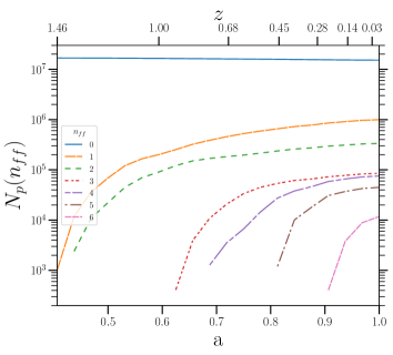
Figure 1: Number of particle $N_{\rm p}$ that experienced $n_{\rm ff}$ flip-flops as a function of scale factor $a$. Redshift is shown on the top axis.

Figure 1 provides a sense of the evolution of the structure in the simulation at the nonlinear stage. It shows the monotonic growth of the number of particles experienced flip-flops and the decrease of the number of particles with zero flip-flops $N_{p}(n_{\rm ff},a)$. It is also worth noting an orderly behavior of $N_{p}(n_{\rm ff},a)$: $N_{p}(n_{\rm ff},a)>N_{p}(n_{\rm ff}+1,a)$ for all $a$ and $N_{p}(n_{\rm ff},a_{2})>N_{p}(n_{\rm ff},a_{1})$ for all $n_{\rm ff}$ if $a_{2}>a_{1}$. The number of particles drops from $\approx 10^{6}$ at $n_{\rm ff}=1$ to $\approx 10^{4}$ at $n_{\rm ff}=6$. It is worth stressing that the number of vertices in the caustics in the region we discuss in section 5 is 10–100 times less as Table 1 in Appendix A indicates.

4 Identification of caustics in numerical simulations

Finding caustics in numerical simulations by the ZA as well as by N-body techniques could be made by various methods. One can do this by analyzing singularities of the eigenvalue fields of the deformation tensor $\partial s_{i}/\partial q_{j}$, where $s_{i}(\mathbf{q},t)=x_{i}(\mathbf{q},t)-q_{i}$. In the case of the ZA it is simply $D(t)s_{i}(\mathbf{q})$ in Equation 2.1. In the case of N-body simulations it requires numerical calculation of the positions of the particles at time $t$. The passage of a particle through the singular stage can be registered through the change of sign of the Jacobian $J$ (Equation 2.2), see e.g. [26, 14]. This method allows to count how many of times a particle passed through the caustic state which is equivalent to the number of flip-flops computed for each particles. The probe of the geometry and topology of caustics requires to analyze the spacial structure of the eigenvalue fields [18, 19, 20].

In this paper we will use a different method of finding caustic surfaces directly from the Lagrangian triangulation [5, 6]. First we need to evaluate the volume of every tetrahedron in the tessellation. It can be done by computing the following determinant for each tetrahedron

$$d=\begin{vmatrix}x_{1}&y_{1}&z_{1}&1\\ x_{2}&y_{2}&z_{2}&1\\ x_{3}&y_{3}&z_{3}&1\\ x_{4}&y_{4}&z_{4}&1\end{vmatrix},$$ (4.1)

where $x_{i},y_{i},z_{i}$ are the coordinates of four vertices of the tetrahedron. It is easy to see that the determinant $d$ can be either positive or negative because changing the order of the vertices results in swapping a pair of rows in the determinant resulting in the change of its sign. Each determinant $d$ in the tessellation can be made positive at the initial time. Thus the volume of every tetrahedron becomes $V_{i}=d_{i}/6$. Similarly to the Delaunay triangulation, the Lagrangian algorithm considers the particles as the tracers of collision-less DM fluid. However, contrary to the Delaunay triangulation, the initial tessellation remains intact during the entire evolution regardless of the changes of the mutual distances between the particles. In particular, the order of vertices remains the same in each tetrahedron.

In the course of time a vertex of a tetrahedron can cross the opposite face. This results in the change of the sign of $d$ indicating that the tetrahedron has turned inside out. If two neighboring tetrahedra sharing a common face have opposite signs of $d$ then the common face is an element of the caustic surface and thus becomes a cell in the triangulation of the caustic surface. The caustics identified by this method are A2 singularities according to Arnold’s classification. All higher order singularities are singular lines and points on caustic surface A2. For instance cusps are A3 singularities on the curves lying on the surface A2.

In our code the determinant $d$ is calculated for all tetrahedra only at every output time but not at every time step of the simulation. Therefore the numbers of the tetrahedra’s flip-flops are not available. However, finding the triangle elements of caustics requires only the signs of the tetrahedra volumes. Hence the caustics can be obtained without recording the whole history of flip-flopping. Instead of computing flip-flops of tetrahedra we do it on particles because it is easier to implement numerically at every time step [14].

Identifying caustics in Eulerian space is getting complicated because they often cross each other. If the number of flip-flops was known for each tetrahedron then caustic triangles could be assigned the mean number of flip-flops of two parent tetrahedra as a proxi assisting the search of caustic surfaces. The caustic elements carrying the same half-integer flip-flop tag would be separated out as an individual caustic surface. But we compute flip-flops only for the vertices of caustic triangles. In order to relieve this problem we have devised two diagnostics.

Anticipating the number of flip-flops to grow from external to internal caustics we assign the mean number of flip-flops computed on the vertices of the caustic triangles $n_{\rm ff}^{\triangle}\equiv{1/3}\sum_{i=1}^{3}n_{\rm ff}(v_{i})$ to the triangles as a diagnostic helping to isolate caustics of different generations. We also expected that the triangles of the internal caustics must be on average smaller by size. We compute the length of the longest edge of the triangle $l_{\rm max}\equiv max(l_{1},l_{2},l_{3})$ where $l_{1},l_{2},l_{3}$ are the edges of a caustic triangle. Both expectations have proved to be correct as we show in section 5.

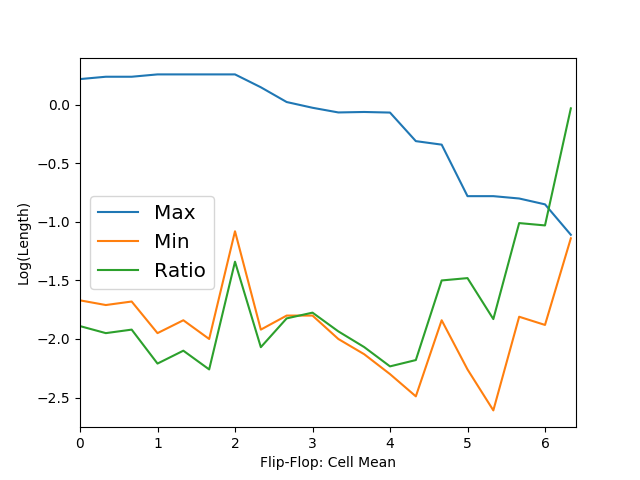
Figure 2: The mean of the longest $\langle l_{\rm max}\rangle$ and shortest $\langle l_{\rm min}\rangle$ edges in caustic triangles as a function of $n_{\rm ff}^{\triangle}$ (Equation 4.2) along with the ratio $\langle l_{\rm min}\rangle/\langle l_{\rm max}\rangle$.

We evaluate the mean values of $l_{\rm max}$ as a function of $n_{\rm ff}^{\triangle}$ by averaging over all triangles with the same values of $n_{\rm ff}^{\triangle}$

$$\langle{l_{\rm max}}\rangle(n_{\rm ff}^{\triangle})={1\over N_{\triangle}}\sum_{i=1}^{N_{\triangle}}max(l_{1}^{(i)},l_{2}^{(i)},l_{3}^{(i)}).$$ (4.2)

We also define $\langle{l_{\rm min}}\rangle(n_{\rm ff}^{\triangle})$ similarly to Equation 4.2. Figure 2 shows both $\langle l_{\rm max}\rangle$ and $\langle l_{\rm min}\rangle$ along with their ratio $\langle l_{\rm min}\rangle/\langle l_{\rm max}\rangle$. The figure shows that $\langle{l_{\rm max}}\rangle(n_{\rm ff}^{\triangle})$ is monotonically decreasing from $\langle{l_{\rm max}}\rangle(n_{\rm ff}^{\triangle}=2)$ by more than an order of magnitude at $n_{\rm ff}^{\triangle}=6.3$. The caustic triangles become not only smaller but also more compact since the ratio $\langle l_{\rm min}\rangle/\langle l_{\rm max}\rangle$ increased from $\sim 10^{-2}$ at $n_{\rm ff}^{\triangle}=0$ to almost $\sim 1$ at $n_{\rm ff}^{\triangle}=6.3$. We use the both as additional diagnostics helping to isolate independent caustic surfaces.

Our tessellation decomposes each elementary cube in five tetrahedra [5]. There are two kinds of tetrahedra in Lagrangian space: the central one with volume $V_{c}=l_{0}^{3}/3$ and four corner tetrahedra with volumes $V=l_{0}^{3}/6$ where $l_{0}=L/N$. Here $L$ is the size of the box in units of $h^{-1}$ Mpc and $N^{3}$ is the number of particles in the simulation. Initially the central tetrahedron is regular with edges $l_{c}=\sqrt{2}\,l_{0}$. Four equal corner tetrahedra have three edges of length $l_{1}=l_{0}$ and three of length $l_{2}=\sqrt{2}\,l_{0}$.

5 Caustics in a high sampling simulation

We discuss only the final stage of the simulation corresponding to $a=1$ and focus on the structure that has reached the most advanced stage in dynamical evolution. The caustic surfaces in the full simulation box are shown in figure 3. There are only a few largest caustic structures with more than a thousand of caustic elements i.e. caustic triangles/cells and caustic vertices/particles. However, the overall abundance of structures is not much different from that in the HDM simulations in [33].

The geometry of the external caustic shells separating a multi-stream regions from the single-stream region is typically simpler than that of the internal caustics. They resembles the typical caustic structures in the ZA simulations. The internal caustics are much more complex and their shapes have not been systematically studied in cosmological N-body simulations. Identifying and examining some of them is the major goal of our study.

The most dynamically advanced part of the caustic structure in this simulation is highlighted by color in figure 3. It consists of a filament and two haloes at the both ends resembling a dumbbell. It is embedded in the external cylindrical caustic with significantly greater diameter than the internal filament.

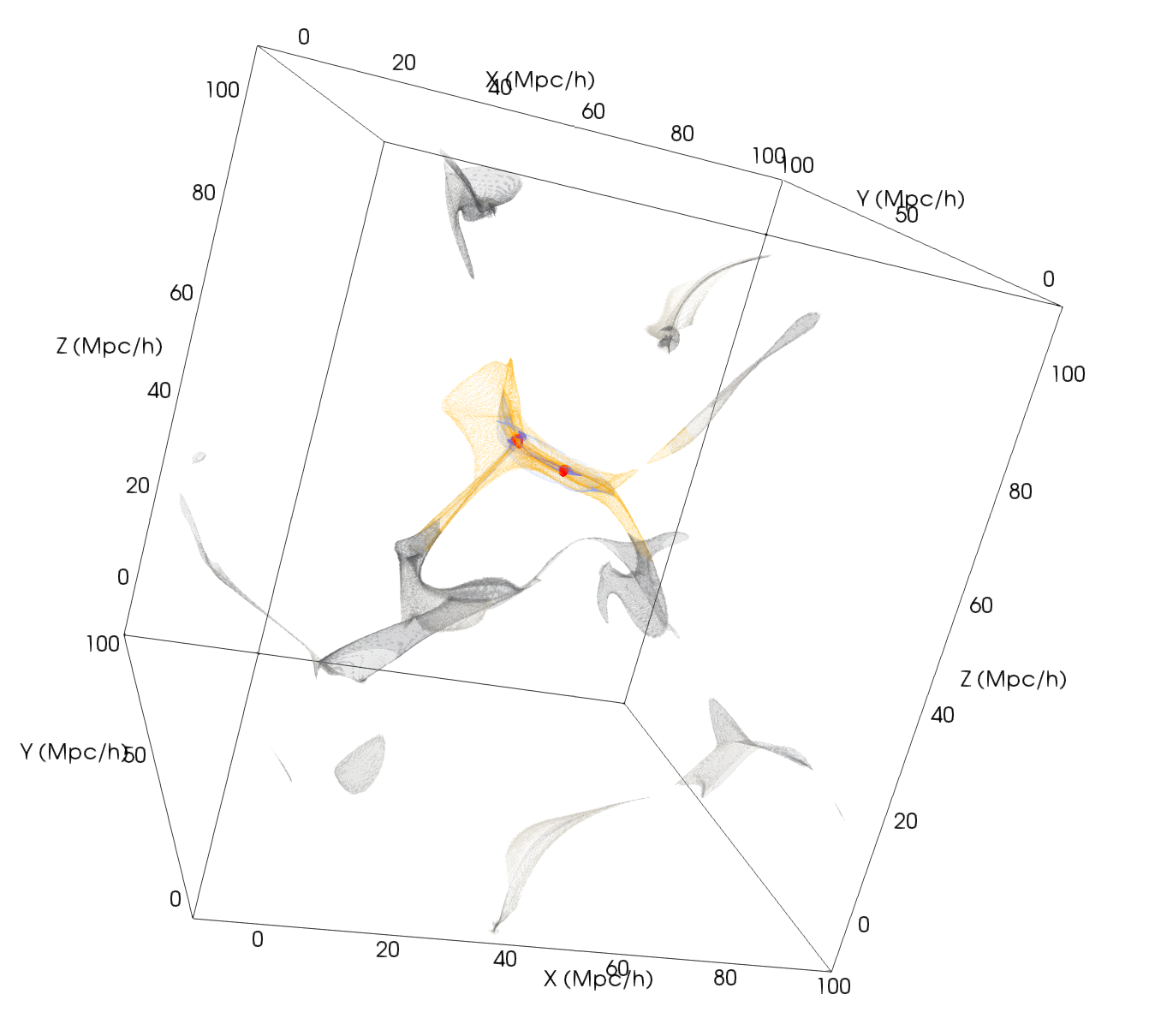
Figure 3: Caustic surfaces in Eulerian space. The colored area marks the region mostly evolved dynamically. It is selected by a spherical clip with the radius of about 20 Mpc/h.

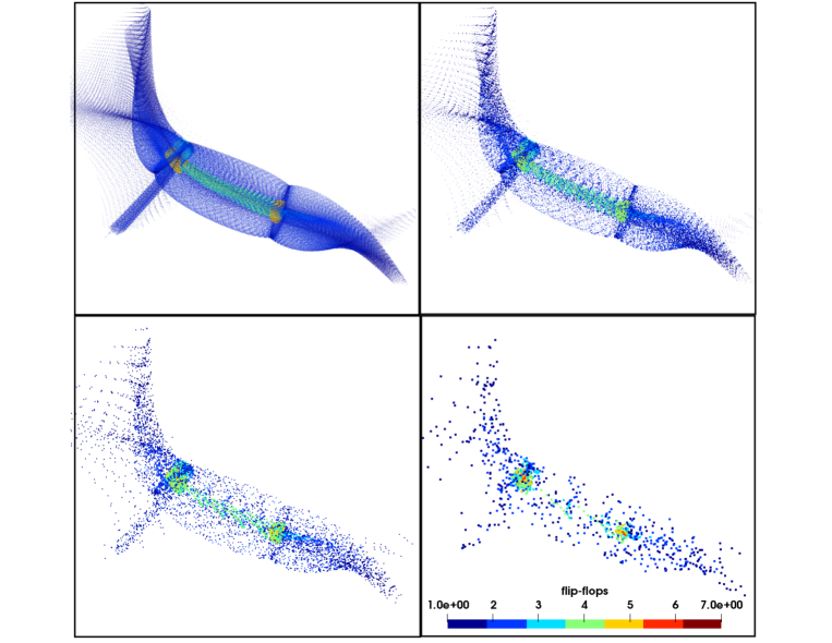
Figure 4: Four images of the structure highlighted by colour in figure 3. It is rendered with different sampling densities parameterized by the ratio of the Nyquist frequency to the cutoff scale $\kappa=k_{\rm Ny}/k_{\rm c}$. Top left: $\kappa=32$. Top right: $\kappa=16$. Bottom left: $\kappa=8$. Bottom right: $\kappa=4$ Colour encodes the number of flip-flops passed by each particle as indicated by the legend. Only particles that passed at least one flip-flop are shown.

5.1 Why do we need a high mass resolution simulation?

A short answer is trivial: it is impossible to render or characterize a complex geometry with insufficient number of elements. Long time ago is was shown in two-dimensional high-resolution simulations that the complexity of the structure can be revealed only with sufficiently high mass resolution [24]. Using a tetrahedral tessellation of the three-dimensional manifold allows to improve rendering the DM density with more numerous tetrahedra centers that discloses the structure in considerably more detail [5, 6]. Moreover by exploiting this technique it is possible to devise an improved particle-mesh technique [7, 9]. The new technique allows to follow the evolution even in regions with very strong mixing.

Figure 4 provides a visual illustration of the importance of mass resolution by showing exactly same structure rendered with different number of particles. It is useful to look at the ratio of the cutoff scale to the mass resolution scale $\kappa=k_{\rm Ny}/k_{\rm c}$ where $k_{\rm Ny}=(N/2)(2\pi/L)$ is the Nyquist frequency and $k_{\rm c}=4(2\pi/L)$ the cutoff wave number. The top panels correspond to $\kappa=32$ and 16 on the left and right side respectively the bottom panels to $\kappa=8$ and 4 on the left and right side respectively. In the majority of cosmological N-body simulations of the CDM universe the cutoff of initial power spectrum happens naturally at $\kappa\sim 1$. The rich structure in the top-left panel ($\kappa=32$) is steadily fading-out as $\kappa$ is decreasing. Only two weak remnants of the haloes at the both ends of the green filament can be identified in the bottom-right panel corresponding to $\kappa=4$.

It is instructive to compare figure 4 with the filament shown in the dot plots of figure 2 obtained in three simulations with a range of mass resolutions and much smaller force softening length $R_{\rm s}=0.04h^{-1}$  Mpc [33] .

5.2 Caustics in two-dimensional slices

First, we demonstrate that the structures shown in figure 3 represent a set of physical surfaces. Each caustic triangle is found and plotted absolutely independently of all the rest. An assumption that a set of independent triangles form a continuous surfaces inevitably predicts that the cross-section of a plane with this set of triangles must be a discrete set of continuous curves. Figure 5 showing two orthogonal infinitesimal slices through the coloured caustics in figure 3 unambiguously confirms this prediction.

Two upper panels show the same infinitesimal slice through the both red blobs in figure 3. Two lower panels show the slice across the structure in the middle part. It is interesting that the two-dimensional structure shown in the upper panels is remarkably similar to figure 4 obtained in a high resolution two-dimensional N-body simulation [24] . This is an evidence that although the number of topological types of caustics in 3D is greater than in 2D nonetheless there are some similar types as in the case of the ZA.

The color bars show the range of $\log(l_{\rm max}/l_{0})$ in two panels on the left-hand side of figure 5 where $l_{\rm max}$ is the longest edge of the caustic triangles crossed by the plane. In the panels on the right-hand side colors show the mean number of flip-flops on the caustic triangles. We are reminding that $\log(l_{\rm max}/l_{0})=\log(\sqrt{2})\approx 0.15$ and $n_{\rm ff}^{\triangle}=0$ at the initial time.

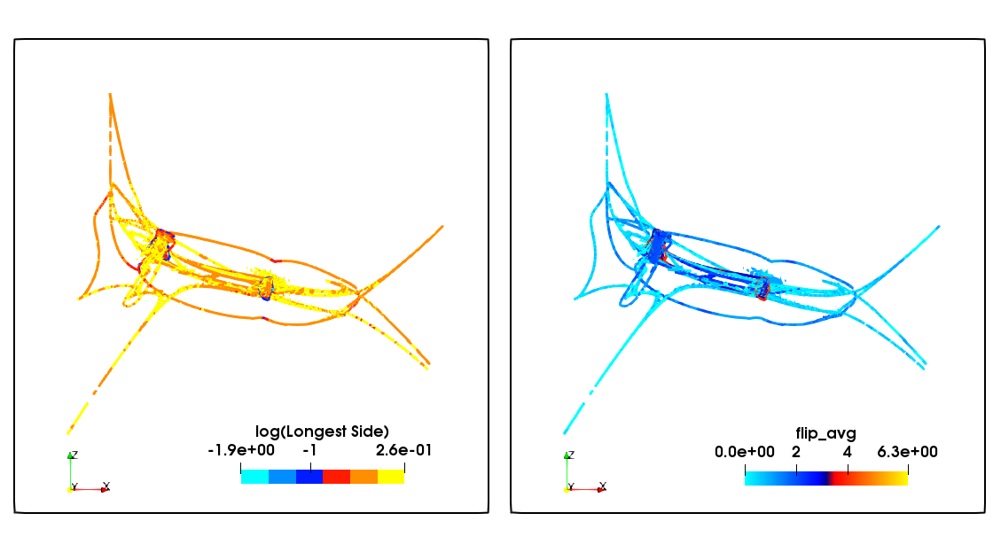
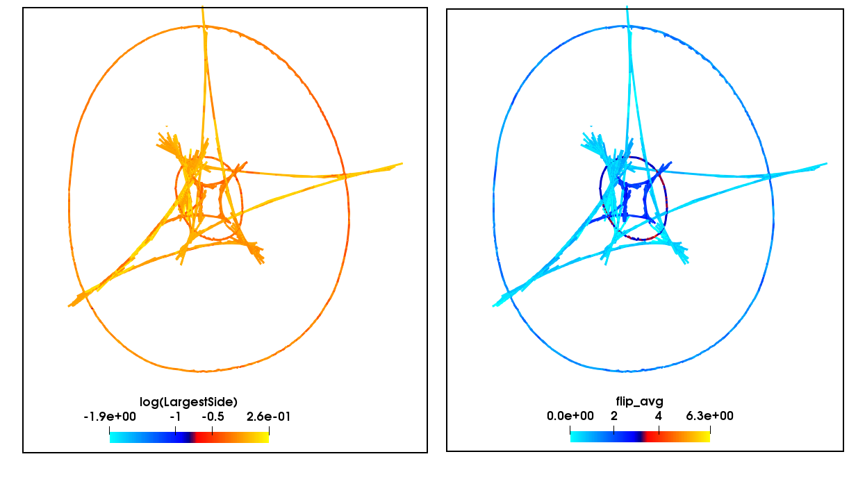
Figure 5: Two razor thin approximately orthogonal slices of the highlighted region in figure 3. Top panels: a slice passing through two yellow halos in figure 4. Bottom panels: a slice across the middle of the green filament in figure 4. Colour encodes $\langle{l_{\rm max}}\rangle$ (left panels) and $n_{\rm ff}^{\triangle}$ (right panels). Note that the linear scales are different in top and bottom panels.

All panels demonstrate an apparent correlation of large triangles (yellow and brown curves on the left) with low counts of flip-flops (cyan and blue curves on the right) in agreement with the claims in section 4 and figure 2. Unfortunately, the correlation of small triangles (cyan and blue lines on the left) with high counts of flip-flops (yellow and brown lines on the right) is not obvious. However, by magnifying the figure one can see that the cyan and blue curves on the left corresponding to small triangles are covered by the yellow and brown curves corresponding to large triangles. A similar remark can be made for small and large values of $n_{\rm ff}^{\triangle}$ in the right panels. The arrangement of the caustics in Eulerian space – in particular, in the higher panels of figure 5 – are substantially more cumbersome than that in Lagrangian space as we discus it briefly bellow. Two lower panels of figure 5 reveal two remarkably smooth concentric ovals. Thus, the figure suggests that the corresponding caustics in three-dimensional space are two smooth approximately coaxial oval cylinders which can be seen also in figure 6: external in magenta and internal in yellow. This is a clearly non-linear feature having no analogue in the ZA. The both ends of the internal cylinder are compact quasi-spherical closed shells also have not seen in the ZA. The quasi-cylindrical caustic – green in figure 4 – with two compact closed caustics – red in figure 3 or yellow in figure 4 – at the cylinder ends resemble a dumbbell. This structure will be discussed in far greater detail later in section 5.3.

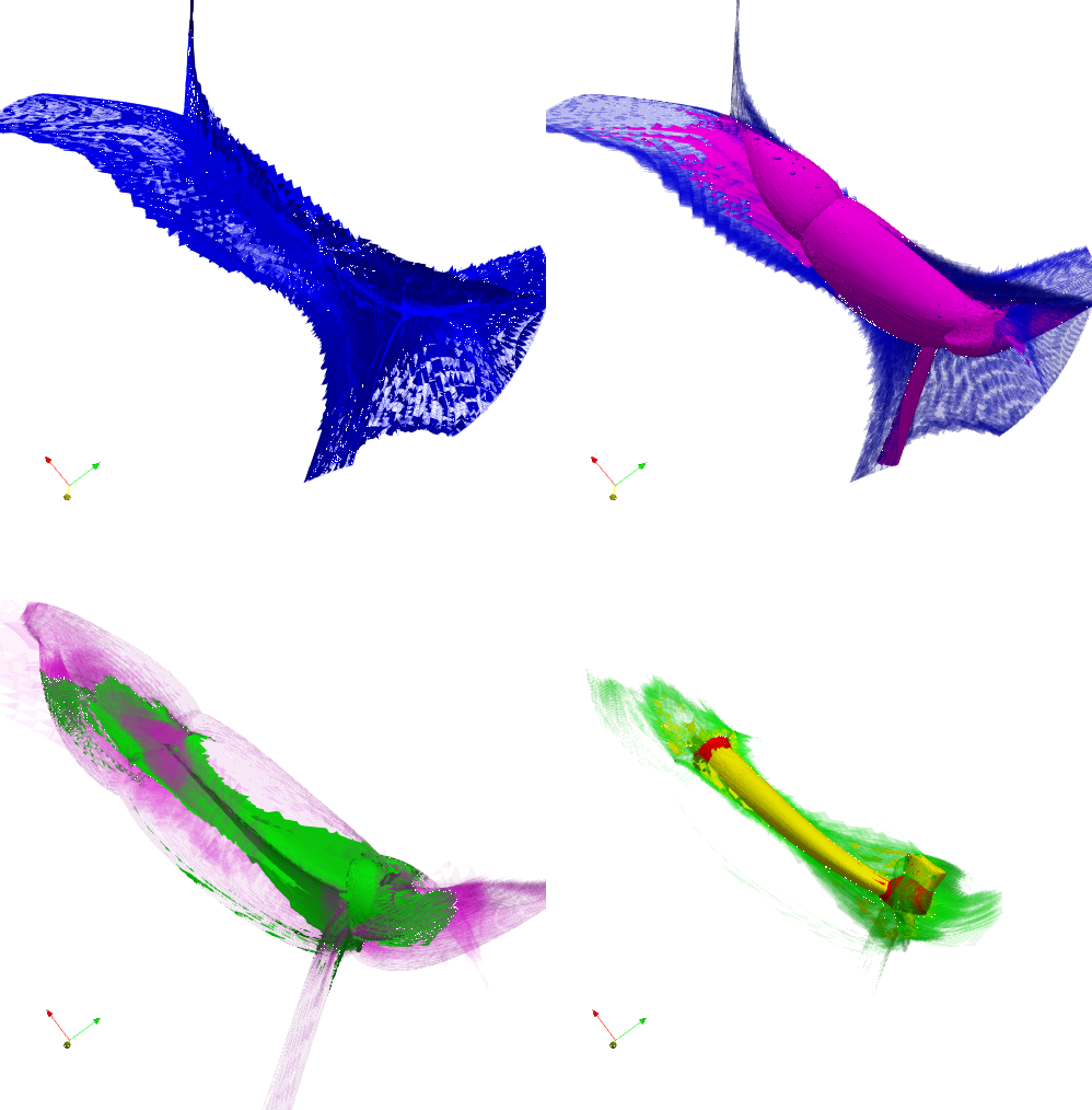
Figure 6: Four images of the caustics in the highlighted part of figure 3. Five caustic shells are shown in blue, magenta, green, yellow and red. The surfaces in blue and magenta are the outermost caustics in the region. Two lower images have been zoomed in. The distance between two red halo shells seen in the lower right image is about 10 Mpc/h.

5.3 Shapes of caustics in three-dimensions

5.3.1 Eulerian space

Now we will discuss in detail the shapes of the internal caustics in three dimensions. The caustic that are discussed in this paper are certainly only coarse-grained approximations. However, it is worth stressing that even coarse-grained caustics are truly real physical objects although up to accuracy of the physical model. Therefore caustics must be unambiguously distinguished from contour plots of the density fields because the contour levels can be arbitrarily chosen. A distribution of caustics in space represents a specific intermittent phenomenon in the sense that it is a physical system that has only two states: one is a discrete set of caustic surfaces and the other is empty space. Alternatively it can be considered as a purely geometric structure made up from two-dimensional surfaces. Both require very specific methods of analysis. The caustics change their positions with time but physical velocities of the particles – the vertices of the triangulated surface – cannot be considered as the velocities of the caustic because caustic surfaces evolve with phase velocities.

As we mentioned earlier in our approach the caustic surfaces consist of mutually independent triangles each of which is fully defined by two neighboring tetrahedra. Figure 5 suggests that setting thresholds on $n_{\rm ff}^{\triangle}$ (Equation 4.2 and the text above it) may help to isolate particular parts of the total caustic surface. As we describe in Appendix A each pattern shown in figure 6 is specified by three or four components selected by a single value of $n_{\rm ff}^{\triangle}$ (Table 1 ).

The colored patch in figure 3 is magnified and dissected into five distinct patterns displayed in figures 6. Two shells in blue and magenta shown in two upper panels are the outermost caustics in the highlighted region of figure 3. The upper right image shows that the caustics in blue and magenta cross each other. In this image the blue caustic is painted with low opacity that allows to see more of the caustic in magenta. The middle part of the caustic in magenta looks approximately as a cylinder or tube. The cross section plane passing through its axis gives an idea of its three-dimensional contour (see the lower panels in figure 5). Then the caustic in magenta is plotted with low opacity in order to see the internal caustic in green is shown in the bottom left panel of figure 6.

Two red caustics in bottom right image are compact closed surfaces – neither spherical nor ellipsoidal. Located exactly at the ends of the yellow tube they form a configuration made by two haloes connected by a cylindrical filament bounded by yellow caustic. We label this structure as a dumbbell. The red halos are separated by the distance of approximately 5 Mpc/h. We are suggesting that the red caustics would be good candidates for the outermost convex caustic of the haloes that could be called ’splashback caustics’ on cluster scales in analogy with ’splasback radii’ on galactic scales [21, 22, 34]. We provide additional arguments in section 6 where we discuss the velocity fields as well as kinetic and potential energies in one of them.

Very smooth shapes of the red and yellow caustics suggest that they are controlled by smooth local gravitational potential which also controls the very smooth shell in magenta. This may explain why these components in figure 6 are so different from caustic structures known in the ZA. However, they are inside of green and blue shells which look more familiar since they resemble some of the caustics predicted by the ZA. They are probably formed by the streams falling with the velocities mostly acquired in the large-scale gravitational potential and therefore form the caustic structures more similar to the caustics in the ZA.

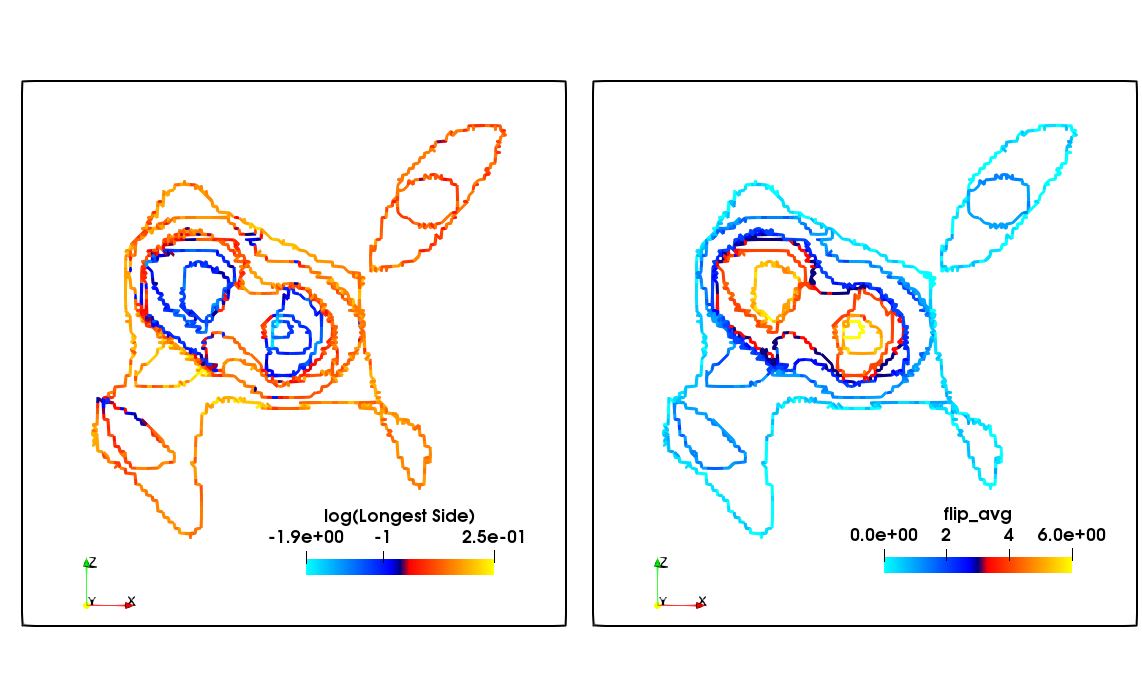
Figure 7: Four images on the left are the caustics in a spherical clip with the radius about 26 Mpc/h in Lagrangian space approximately corresponding to the caustics in figure 6. Two right panels show a razor thin slice through the full set of caustics in Lagrangian space roughly corresponding to the slice in the top of figure 5. The colour scale is the same as in figure 5. Note the nesting structure of caustic surfaces in Lagrangian space.

There are small internal caustic structure of the next generation within the red caustics. Their shapes are resembling the Zeldovich pancakes with thickness around 0.15 Mpc/h. The thickness is smaller than the force softening scale therefore their shapes may be artefacts of low force resolution.

5.3.2 Lagrangian space

Figure 7 shows the progenitors of five caustic shells shown in figure 6 in Lagrangian space. In addition two black caustic shells inside the red caustics are also displayed. The figure confirms the suggestion made at the end of the previous section that the caustics surfaces in Lagrangian space represent the nesting structure that may be easier to disentangle than in Eulerian space. For instance, when two-dimensional slices in figure 5 were discussed we mentioned that the triangles with small $\langle{l_{\rm max}}\rangle$ (left-hand panels) and high $n_{\rm ff}^{\triangle}$ (right-hand panels) could not be easily seen because they were obscured by the triangles with large $\langle{l_{\rm max}}\rangle$ and low $n_{\rm ff}^{\triangle}$. But two right panels in figure 7 demonstrate the entire ranges of the both $\langle{l_{\rm max}}\rangle$ and $n_{\rm ff}^{\triangle}$. Thus, the internal higher generation (high $n_{\rm ff}^{\triangle}$ – red-yellow curves) streams are assembled from small triangles (small $\langle{l_{\rm max}}\rangle$ – blue-cyan curves) in the corresponding panels of figure 7.

Comparing the caustic structure in Lagrangian space with their Eulerian counterparts one may conclude that it is much easier to disentangle them in Lagrangian space than in Eulerian space especially in dense crowded regions. This is because the caustics typically intersect with each other in Eulerian space but do not in Lagrangian space where they are described by a single value function. However, they may have common lines where $\lambda_{1}(\mathbf{q})=\lambda_{2}(\mathbf{q})$ or $\lambda_{2}(\mathbf{q})=\lambda_{3}(\mathbf{q})$ [18, 19].

6 The dumbbell structure

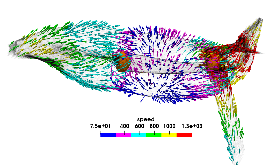
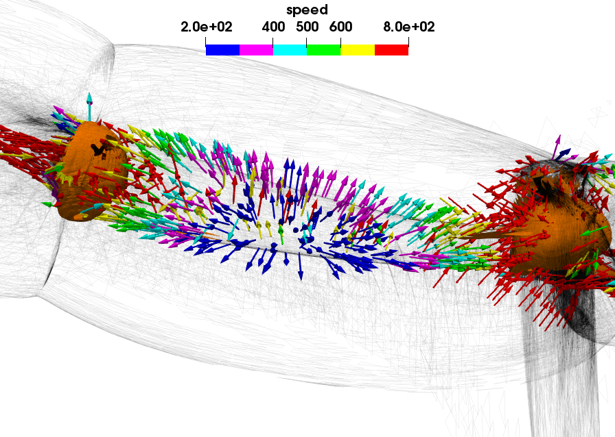
Figure 8: Left panel: The velocities of the vertices of the external caustic shell shown in figure 6 in magenta. Note that the arrows render only velocity directions. The speeds of particles are encoded by colour. The set of arrows selected by statistically uniform spatial distribution for clarity. Two brown blobs are the halo caustic shells. Brown colour allows better see the high speed particles in red. Right panel: The velocities of the vertices of the internal caustic shell. Note the difference in colour scales.

6.1 Velocity streams

First, we consider the velocities of the particles that are vertices of the triangle elements of two caustics in magenta and yellow in figure 6 or the external and internal caustics respectively shown as semitransparent gray surfaces in figure 8. It is worth stressing that the velocities of the caustic vertices are not simply related to the propagation of caustic surfaces because the latter cannot be described by the physical velocity but requires the phase velocity.

The velocities of particles are shown by a set of arrows attached to a subset of the caustic vertices. For clarity the subset of the vertices was selected according to statistically uniform spatial distribution. Therefore the appearance of the arrows does not reflect the actual density of the caustic vertices. The arrows are of a constant length and the speed is encoded by colour according to the legends in the figure. The caustic surfaces in gray are very smooth between the haloes (see also figure 5) but outside they have rather complex connections with other parts of the caustic web. Those are better seen in figure 3.

The velocity patterns are similar in both caustics. They demonstrate the steady growth of speed toward the haloes - the vector colours change from blue to red. There is a relatively narrow region on both caustics where the longitudinal component of the particles changes the sign.

The counts of flip-flops allow a qualitative description of the trajectories of particles as a sequence of flip-flops that are happening in the caustics. For instance, the particles that have reached the yellow caustics had experienced the first four flip-flops in the following order of the caustics referred to by the colours in figure 6: blue, magenta, green, and yellow. The slice approximately through the middle point between the haloes in orthogonal direction is shown in lower panels of figure 5. The particles experiencing the first collapse to a caustic form the exterior star-like configuration in cyan in the right-hand panel. The particles experiencing the second caustic event form the exterior oval. The third collapse corresponds to the interior star-like configuration and the fourth collapse is happening in the interior oval. It would be naive thinking that the particles have passed through the caustics shown at one instant of time because it takes a considerable time so the caustics could evolve. Nevertheless it gives some hint about the type of caustic surfaces. We continue the story in the next section where we analyze the velocity structure of one of the halos.

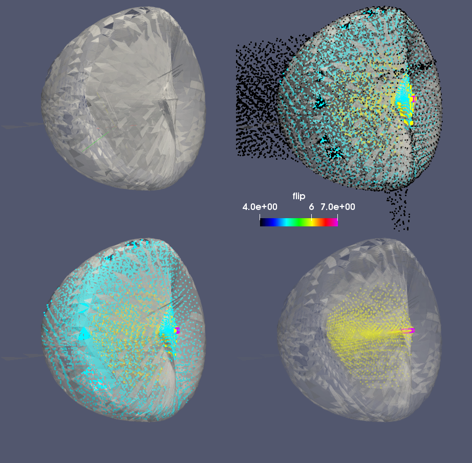
Figure 9: An illustration to building the grid template of the halo identified by a caustic shell. Top left panel: the caustic shell. Top right panel: the shell together with all the particles with flip-flop counts from four to seven in a small box of size 3/h Mpc. The colour encodes the number of flip-flops: black - 4, cyan - 5, yellow - 6, and red - 7 flip-flops. Bottom left panel: the shell and the particles with flip-flop counts from five to seven. Bottom right panel: the shell and the particles with flip-flop counts from six to seven.

6.2 The halo bounded by a caustic

Here we consider the structure of the streams inside one of two brown caustic shells shown in figure 8. The shell is in the left in both images. The caustic is closed and convex however, it’s shape neither spherical nor ellipsoidal. Therefore we will begin with an explanation how the particles in all streams were found within the caustic shell.

6.2.1 Building a mask for asymmetrical halo

In order to speed up computing we begin with selecting all the particles in a small cubic subbox of size 3 Mpc/h that completely encloses the caustic boundary. The box contains 79563 particles with the total mass $3.9\times 10^{14}M_{\bigodot}/h$. Figure 9 shows the caustic shell in top-left panel. The image in top-right panel shows the caustic surface and all particles in the box with $n_{\rm ff}\geq 4$. Some particles coloured in black with $n_{\rm ff}=4$ are outside of the caustic shell but as we will see later the most of such particles are inside. Two images in the bottom panels show the caustic shell and all the particles in the box with $n_{\rm ff}\geq 5$ and $n_{\rm ff}\geq 6$ on the left and right of the figure respectively. Therefore the particles with $n_{\rm ff}\geq 5$ can be used for building the mask that later may be used for selecting all particles inside the caustic shell. In our case we map the particles with $n_{\rm ff}\geq 5$ into an auxiliary cubic grid using the nearest-grid-point (NGP) scheme to label the grid points inside the caustic shell. The labeled grid points make the geometrical template for the halo based only on physics with no additional assumptions or parameters. The last step is to identify all particles in the subbox that are near the labeled grid points.

The red, blue and black histograms on the left of figure 10 show the number of particles inside and outside of the caustic boundary as well as the total in the subbox respectively. The blue histogram clearly shows that there are no particles outside the shell with $n_{\rm ff}\geq 5$ and the most of particles with $n_{\rm ff}=4$ are inside the shell. The red histogram shows that the number of particles with $n_{\rm ff}=4$ and $n_{\rm ff}=3$ inside the shell is greater than that outside the shell however, if $n_{\rm ff}<3$ the opposite is correct. The distribution of the distances of the caustic vertices from the center of mass of the caustic particles shown on the right of figure 10 provides some notion of its asymmetry.

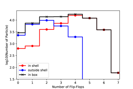
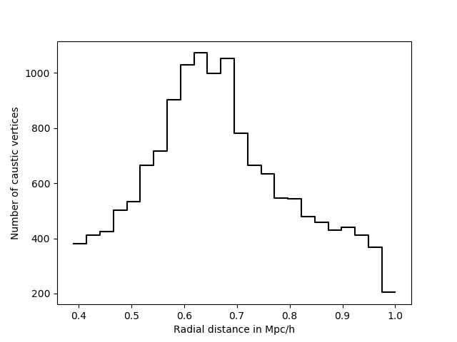
Figure 10: Left panel histograms: the number of particles with different counts of flip-flops. The labels with the colour of each histogram indicate how the particles were selected. Right panel histogram: the number of caustic vertices vs. the distance from the center of the caustic shell.

The total volume of the template region is $V_{\rm templ}=$ 2.4 (Mpc/h)³ which is a good approximation of the volume within the caustic shell.

The counts of particles with 7, 6, 5 , 4 flip-flops within the caustic shell are 59, 3893, 12158, and 15817 respectively. The total number is 31927 making the mass within the shell $M(n_{\rm ff}\geq 4)=1.6\times 10^{14}M_{\bigodot}/h$. However, the shell contains also streams with 0, 1, 2, and 3 flip-flops with 630, 805, 4037, and 7325 particles respectively. Thus the total number of all particles within the caustic shell is 44724 and the mass becomes $M(0\leq{n_{\rm ff}}\leq 7)\approx 2.2\times 10^{14}M_{\bigodot}/h$. Dividing the mass by the volume within the caustic shell we estimate the mean density within the shell as $9.2\times 10^{13}M_{\bigodot}$h²/Mpc³ which is about thousand times greater than the mean mass density in the universe.

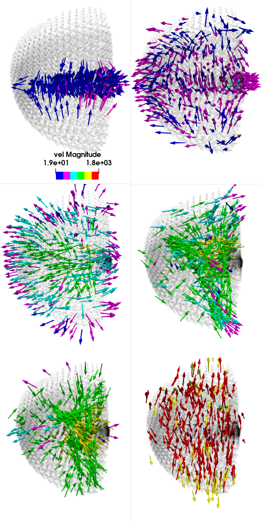
Figure 11: Velocities in the streams selected by the flip-flop count $n_{\rm ff}$. Randomly selected subsamples of the particles within the caustic shell are shown in six panels. Top-left panel : $n_{\rm ff}=7~{}{\rm or}~{}6$. Top-right panel: $n_{\rm ff}=5$. Middle-left panel : $n_{\rm ff}=4$. Middle-right panel: $n_{\rm ff}=3$. Bottom-left panel : $n_{\rm ff}=2$. Bottom-right panel: $n_{\rm ff}=1~{}{\rm or}~{}0$. The caustic is shown by semi transparent gray surface. Vectors show only the direction of the velocities. Colour encodes the ranges of speed in km/s: 19 $<$ blue $<$ 316 $<$ magenta $<$ 613 $<$ cyan $<$ 910 $<$ green $<$ 1206 $<$ yellow $<$ 1503 $<$ red $<$ 1800.

6.3 Velocity field within the caustic shell

Figure 11 illustrates the velocity fields in the streams selected by the values of flip-flops. For the purpose of clarity all arrows have the same length thus showing only the directions of the velocities of a randomly selected particle set for every stream. The colour encodes the speed. The discrete set of colors represents equally spaced intervals in the range from the minimum to maximum of the particle speeds as described in the caption to figure 11. The caption of the figure provides the description of the images.

The velocity streams seems to form the patterns of four types.

1. The slowest particles with 7 and 6 flip-flops - blue in top-left panel show the infall of particles on the pancake-like caustic structure.

2. The particles with 5 and 4 flip-flops shown in top-right and left-middle panels seem to relate mostly to the caustic shell. The particles in magenta and blue indicate that the speed decreases when the particles approach the caustic boundary from inside.

3. Two panels dominated by green arrows (right-middle and left-bottom panels) seem to fall into the central part and building up another caustic structure with different geometry than the caustic shell. Compare with the images in bottom panels of figure 5.

4. Finally the fastest particles (yellow and red on the right side of the bottom row) seem to zoom through the caustic shell practically ignoring its gravitational field.

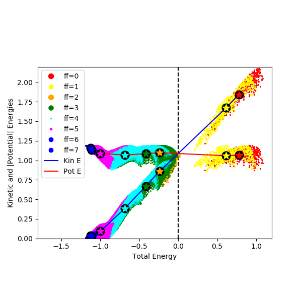
Figure 12: Kinetic and negative potential energies of the particles in the halo are plotted as the functions of the total energy shown on the horizontal in units of $10^{59}$ ergs/h. The streams are indicated by different colours. The coloured dots in the legend are proportional to the sizes of the points in the plots. Stars in black circles show the corresponding mean values for each stream. The blue and red lines connecting the stars show the kinetic and potential energies respectively. The vertical dashed line marks zero of the total energy. The mean energies of the stream with $n_{\rm ff}=3$ (in green) approximately satisfy the virial ratio.

6.4 The energy of the halo

6.4.1 The energy distribution in the halo

The distribution of particle energies in the halo provides an additional diagnostic of its dynamical structure. We evaluate kinetic, potential and the total energies for all particles in the halo: $K_{\rm i}=0.5m_{p}v_{i}^{2}$, $U_{\rm i}=-Gm_{p}^{2}\Sigma_{j=1}^{N_{p}}|{\bf r}_{i}-{\bf r}_{j}|^{-1}$ (${\rm j}\not={\rm i}$) and $E_{\rm i}=K_{\rm i}+U_{\rm i}$ where ${\rm i}$ is the numerical label of a particle. In order to be consistent with the simulation we used a similar condition for softening gravity: in cases when the separation of two particles $|{\bf r}_{i}-{\bf r}_{j}|$ is less than the force softening scale $R_{\rm s}=0.8h^{-1}$  Mpc it was set to $R_{\rm s}$. Figure 12 shows the dot plots of the kinetic $K_{\rm i}$ and negative potential $-U_{\rm i}$ energies as functions of total $E_{\rm i}$ energy. The particles in each stream have its own colour. The colour scheme is the same as in figure 11. The mean potential energy is almost identical in every stream. Therefore the relation between the mean total and kinetic energies is almost exactly linear $\langle K\rangle\approx 1.1+\langle E\rangle$ in units of $10^{59}$ ergs/h.

The mean total energy is steadily decreasing with the grows of the number of flip-flops in the stream. It is negative for streams with $n_{\rm ff}\geq 2$ while $E$ is positive for the streams with $n_{\rm ff}<2$. The virial ratio is $\langle K\rangle/\langle|U|\rangle\approx 1.6$ and $1.7$ for streams with $n_{\rm ff}=1$ and $0$ respectively.

Figure 12 is in agreement with the last statement of the previous subsection. The streams with $n_{\rm ff}\leq 1$ are unlikely gravitationally bound to the halo. Therefore their input into the kinetic energy of the halo can be excluded from the total energy, but the input to the potential energy probably should be kept because it is not affected by their speeds.

6.4.2 The total energy inside the shell

Direct summation of kinetic energies of all particles results in $K=\Sigma_{\rm i}K_{\rm i}=1.27\times 10^{63}$ ergs/h and summation of potential energies over all pairs of particles gives $U=\Sigma_{\rm i}U_{\rm i}=-2.4\times 10^{63}$ ergs. The ratio $K/|K+U|=1.12$ that is 12% higher than the perfect virial ratio. The fraction of kinetic energy by two fastest streams with $n_{\rm ff}\leq 1$ is about 13%. Thus if it is excluded from the total energy balance then the ratio become $K/|K+U|=0.87$ which is 13% less than exact virial ratio. Both seem to be in a reasonable agreement with the virial ratio if one takes into account that the both $K$ and $U$ are supposed to be averaged over time and the dynamical system is assumed to be stable. Neither requirement is exactly fulfilled in this case.

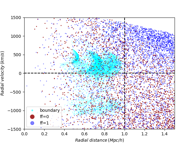
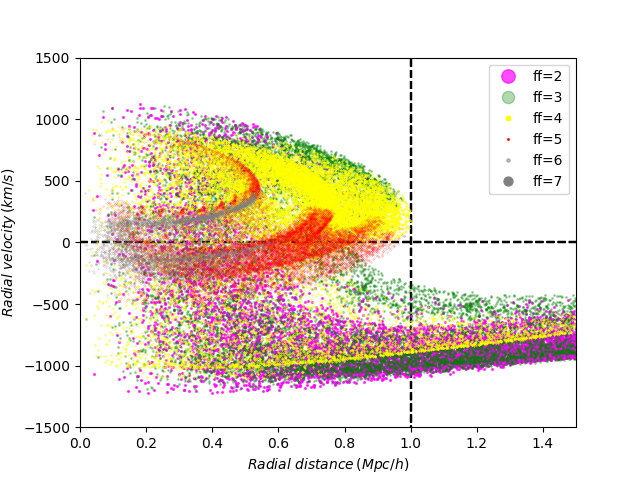
Figure 13: Phase space structure of the halo bounded by the caustic shell. Left-hand panel: two streams with $n_{\rm ff}\leq 1$ (brown and blue) and the boundary particles in cyan. These are the fastest streams in the halo. The gravity of the halo does not noticeably affect these streams. Right-hand panel: five streams with $n_{\rm ff}\geq 2$. Colour encodes the number of flip-flops in every stream. The vertical dashed line indicates the most distant elements of the caustic shell from the halo center of mass. The horizontal dashed line separates inflow and outflow particles. The sizes of the dots in the the colour legend are proportional though not equal to the sizes of the dots in the plots.

6.5 The halo phase space

Unfortunately it is not feasible to illustrate of the velocity field in the caustic shell region in the full six-dimensional phase space. Therefore figure 13 presents a commonly used two-dimensional scatter plots of the radial velocity vs. radial distance from the center of mass of the halo. The radial velocity is measured with respect to the mean velocity of the halo. It is worth emphasizing that the halo is at the origination stage therefore its outermost caustic has a rather irregular shape.

The panel on the left of figure 13 shows two coloured streams (brown and blue) with $n_{\rm ff}\leq 1$ as well as the caustic particles in cyan. The range of the radial velocities of the boundary caustic vertices is also quite large. The distribution of particles seems to show little influence of the halo gravity on these streams. For the particles with zero flip-flops (brown) this is the first run inside a multi-stream region after they crossed the blue caustic from outside of the multi-stream region without experiencing a flip-flop. When they reach the caustic between the three-stream flow from the inside of the three-stream region they experience the first flip-flop and return back to the three-stream flow region. Their color changes from brown to blue in the phase space plot. The next metamorphose of some of them happens when they reach from inside the caustic in magenta. However, no particle with $n_{\rm ff}\leq 1$ that enter the halo is gravitationally bound (see figure 12) to the halo and therefore all of them exit the halo.

The panel on the right-hand side of the figure shows the phase space structure of the streams that become gravitationally bound in the halo. There are three types of particles entering the halo. All of them experienced a flip-flop event in the caustic in magenta. Then some of them directly enter the halo while another group experiences the second flip-flop event in the green caustic and then enter the halo. The third set of particles also experiences a caustic metamorphose in the yellow caustic and only then enter the halo. There are three streams with $2\leq n_{\rm ff}\leq 4$ entering the halo and no particles with $n_{\rm ff}\geq 2$ leave the halo. Since the caustic metamorphoses results in the growth of flip-flops therefore the particles in magenta have experienced two flip-flops, green particles three and yellow particles four flip-flops. The red particles have experienced the fifth flip-flop inside the halo and some of them have became black experiencing the sixth and seventh flip-flops.

The phase space pattern shown on the right-hand side of the figure 13 is typical for haloes. The external streams with $2\leq n_{\rm ff}\leq 4$ are entering the halo with negative radial velocities. They fall on the central region and after passing it the particles get going away with positive radial velocities. This results in the instantaneous leaps of the particles from the lower part onto the upper part in the phase space diagram. The positive radial velocities of the particles are gradually decreasing with the growth of the radial distances. At some distance the fluid elements experience another flip-flop resulting in the formation of the caustic boundary of the halo. Comparing this figure with figure 6 one can anticipate strong anisotropies of the streams entering the halo.

It is worth stressing that the pattern of the phase space shown in figure 13 is strongly affected by the lack of spherical symmetry in the caustic boundary of the halo. It is highlighted by the cyan particles in the left-hand panel of the figure. The caustic boundary operates as a splashback shell described in [22] who stressed that ”the splashback shells are generally highly aspherical, with non-ellipsoidal oval shapes being particularly common”.

7 Summary

The most common approach to the study of the DM structures consists in the analysis of the DM density and velocities in cosmological N-body simulations. We are suggesting a complimentary technique based on identifying and dissecting the caustic structure. Caustics are physical objects while the isodensity contours are mathematical constructions. This is the major difference between caustics and the density contours in DM medium. Both can be used for the description of the structures formed in the non-liner regime. However, the number and values of density levels can be chosen arbitrary that would result in certain arbitrariness of their positions in space and geometrical shapes. In contrast to the density contours both the number of the caustic surfaces, their positions in space and shapes are completely fixed by physics. Therefore the characterization of the DM structures can be done uniquely and unambiguously by locating caustics in cosmological N-body simulations and studying their shapes.

The caustics in our simulation can not be associated with fine grained phase space streams. However the estimate of the DM density from N-body simulations is also only a coarse-grained field. Thus the caustics in N-body simulations should be considered as the coarse-grained approximation obtained from a coarse-grained phase space. These results can not be directly used for the estimates of the density in the fine-grained caustics. On the other hand we show that the coarse-grained caustics can provide reasonably accurate boundaries for the haloes and filaments. Our major findings are summarized bellow.

1. We have identified the caustic structure resembling a dumbbell. It consists of two halo shells connected by a quasi-cylinder caustic. Many examples of this structure can be seen in the density plots in [6, 23, 21]. Often two or three dumbbells sharing the halo between two filaments are arranged in a linear pattern. In our idealized simulation the dumbbell structure is coaxially embedded into another quasi-cylindrical caustic with roughly three times greater diameter. The velocity patterns in the both cylindrical caustics suggest that the particles move toward the haloes with increasing speed. This is an agreement with the prediction made long ago, see e.g. [3]. Finding this structure in a small simulation suggests that it undoubtedly must be ubiquitous.

2. We introduce a novel method of finding DM haloes based on the assumption that the outermost convex caustic is a natural definition of a physical halo boundary. This is similar to the suggestion of [21, 22]. However, our approach has a significant difference. We build caustic surfaces and find the outermost convex caustics. In the course of evolution each particle accumulates the count of flip-flops which is used for identifying different streams [10]. This parameter is also used as additional control of building the caustics since they are boundaries between regions with different number of flip-flops in Lagrangian space. We also used the flip-flop counts in order to identify the streams that are fully within the caustic bound. The particles of such streams were used for building a mask (see figure 10) for the halo. The mask is used for finding all the particles from every stream exactly inside of an asymmetric boundary of the halo. The entire procedure is utterly free of other assumptions about the shape of the boundary. There is also no need in fitting parameters.

3. Knowing all particles inside the halo boundary it was easy to evaluate the mass and kinetic, potential and total energies of the halo: $M(0\leq{n_{\rm ff}}\leq 7)=2.2\times 10^{14}M_{\bigodot}$, $K(0\leq{n_{\rm ff}}\leq 7)=1.27\times 10^{63}$ ergs, $U(0\leq{n_{\rm ff}}\leq 7)=-2.4\times 10^{63}$ ergs and $E=K+U=-1.13\times 10^{63}$ ergs. The ratio $K/|E|=1.12$ is about 12% higher than the virial value.

   It is remarkable that the mean potential energies of the particles in separate streams are very similar while the mean kinetic energy of the particles decreases steadily with increasing $n_{\rm ff}$. The mean kinetic energy of the streams with $n_{\rm ff}\leq 1$ is about 65% higher of absolute value of the corresponding mean potential energy. Therefore it is likely that these streams are not gravitationally bound to the halo. This conclusion is in excellent agreement with the flow patterns of these streams in figure 11 and 13.

4. The two-dimensional phase space of the halo shows that all streams with $2\leq n_{\rm ff}\leq 4$ cross the boundary caustic of the halo with negative velocities with respect to the mean velocity of the halo. No particles with $n_{\rm ff}\geq 2$ exit from the halo. The growth of $n_{\rm ff}$ inside the caustic boundary is the evidence that the halo is gravitationally bound.

Appendix A Identifying distinct caustic structures

A caustic element – a caustic triangle and its vertices – is defined as the shared face of a pair of neighboring tetrahedra having opposite signs of volumes evaluated by Equation 4.1. Each caustic triangle is treated as an independent entity. Therefore the caustic surfaces can be completely determined by a local condition. The mean value of the flip-flop counts on three vertices of a caustic triangle is discrete: $n_{\rm ff}^{\triangle}=n\times(1/3)$ (n – integer) because the number of counts of flip-flops on each vertex is integer. The number of the caustic elements for each value of $n_{\rm ff}^{\triangle}$ is given in Table 1. The table also provides the reference to the colour of five caustics shown in figure 5. Two innermost caustics can be seen only in Lagrangian space shown as black blob inside red caustic shells in figure 7.

Table 1 shows that the most of triangles with $n_{\rm ff}^{\triangle}=1$ are in the caustic in magenta but about 10% of them belong to the blue caustic. Similarly the majority of triangles with $n_{\rm ff}^{\triangle}=2$ are in the green caustic but about 10% belong the the caustic in magenta. Probably it is caused by inconsistency between counting flip-flops on vertices of the tessellation tetrahedra and identifying the caustic triangles by comparing parities of the tetrahedra themselves. We leave solving this problem for the further work.

Table 1. The number of caustic triangles N($\Delta)$ for each $n_{\rm ff}^{\triangle}$.
$n_{\rm ff}^{\triangle}$ 0 1/3 2/3 1 Total Blue N($\Delta)$ 28439 41737 27141 5195 78112 $n_{\rm ff}^{\triangle}$ 1 4/3 5/3 2 Total Magenta N($\Delta)$ 51518 33484 21954 3057 110013 $n_{\rm ff}^{\triangle}$ 2 7/3 8/3 Total Green N($\Delta)$ 49245 23261 14600 87106 $n_{\rm ff}^{\triangle}$ 3 10/3 11/3 Total Yellow N($\Delta)$ 31365 14662 5873 51900 $n_{\rm ff}^{\triangle}$ 4 13/3 14/3 Total Red N($\Delta)$ 20270 7373 2135 29778 $n_{\rm ff}^{\triangle}$ 5 16/3 17/3 6-7 Total Gray N($\Delta)$ 6411 3442 859 373 11085

References

- [1] Y. B. Zeldovich, Gravitational Instabilitity: An approximate theory for Large Density Perturbations, Astron. Astrophys. 5 (1970) 84 [1011.1669].
- [2] Y. B. Zeldovich, A. V. Mamaev and S. F. Shandarin, Laboratory observation of caustics , optical simulation of the motion of particles , and cosmology, Sov. Phys. Uspekhi 26 (1983) 77.
- [3] S. F. Shandarin and Y. B. Zeldovich, Large scale structure of the Universe:, Rev. Mod. Phys. 61 (1989) 185.
- [4] Y. B. Zeldovich and S. F. Shandarin, The Maximum Density in Heavy Neutrino Clouds, Soviet Astronomy Letters 8 (1982) 139.
- [5] S. Shandarin, S. Habib and K. Heitmann, Cosmic web, multistream flows, and tessellations, Phys. Rev. D 85 (2012) 1 [1111.2366].
- [6] T. Abel, O. Hahn and R. Kaehler, Tracing the dark matter sheet in phase space, MNRAS 427 (2012) 61 [arXiv:1111.3944v3].
- [7] O. Hahn, T. Abel and R. Kaehler, A new approach to simulating collisionless dark matter fluids, MNRAS 434 (2013) 1171 [1210.6652].
- [8] O. Hahn, R. E. Angulo and T. Abel, The properties of cosmic velocity fields, MNRAS 454 (2015) 3920 [1404.2280].
- [9] O. Hahn and R. E. Angulo, An adaptively refined phase-space element method for cosmological simulations and collisionless dynamics, MNRAS 455 (2016) 1115 [1501.1959].
- [10] S. F. S. Shandarin and M. M. V. Medvedev, Tracing the Cosmic Web substructure with Lagrangian submanifold, sep, 2014.
- [11] N. S. Ramachandra and S. F. Shandarin, Multi-stream portrait of the cosmic web, MNRAS 452 (2015) 1643 [1412.7768].
- [12] N. S. Ramachandra and S. F. Shandarin, Topology and geometry of the dark matter web: A multi-stream view, MNRAS 467 (2017) 1748 [1608.05469].
- [13] N. S. Ramachandra and S. F. Shandarin, Dark matter haloes: a multistream view, MNRAS 470 (2017) 3359 [1706.04058].
- [14] S. F. Shandarin and M. V. Medvedev, The features of the Cosmic Web unveiled by the flip-flop field, MNRAS 468 (2017) 4056 [1609.08554].
- [15] S. F. Shandarin, The multi-stream flows and the dynamics of the cosmic web, JCAP 5 (2011) 15 [1011.1924].
- [16] J. Stücker, P. Busch and S. D. M. White, The median density of the Universe, MNRAS 477 (2018) 3230 [1710.09881].
- [17] V. I. Arnold, Evolution of singularities of potential flows in collisionless media and transformations of caustics in three-dimensional space, Trudy Seminar imeni G Petrovskogo 8 (1982) 21.
- [18] V. I. Arnold, S. F. Shandarin and Y. B. Zeldovich, The Large Scale Structure of the Universe I. General Properties. One-and Two-Dimensional Models, Geophys. Astrophys. Fluid Dyn. 20 (1982) 111.
- [19] J. Hidding, S. F. Shandarin and R. van de Weygaert, The zel’dovich approximation: Key to understanding cosmic web complexity, MNRAS 437 (2014) 3442 [1311.7134].
- [20] J. Feldbrugge, R. van de Weygaert, J. Hidding and J. Feldbrugge, Caustic Skeleton of Cosmic Web, JCAP 5 (2018) 027 [1703.09598].
- [21] S. More, B. Diemer and A. V. Kravtsov, the Splashback Radius As a Physical Halo Boundary and the Growth of Halo Mass, ApJ 810 (2015) 36 [1504.05591].
- [22] P. Mansfield, A. V. Kravtsov and B. Diemer, Splashback Shells of Cold Dark Matter Halos, ApJ 841 (2017) 34 [1612.01531].
- [23] R. Kaehler, O. Hahn and T. Abel, A Novel Approach to Visualizing Dark Matter Simulations, IEEE 18 (2012) 12 [1208.3206].
- [24] A. L. Melott and S. F. Shandarin, Gravitational instability with high resolution, ApJ 342 (1989) 26.
- [25] A. L. Melott and S. F. Shandarin, Generation of large-scale cosmological structures by gravitational clustering, Nature 346 (1990) 633.
- [26] M. Vogelsberger and S. D. M. White, Streams and caustics: The fine-grained structure of Lambda cold dark matter haloes, MNRAS 413 (2011) 1419 [1002.3162].
- [27] R. Mohayaee and S. F. Shandarin, Gravitational cooling and density profile near caustics in collisionless dark matter haloes, MNRAS 366 (2006) 1217 [astro-ph/0503163].
- [28] A. G. Doroshkevich, Spatial structure of perturbations and origin of galactic rotation in fluctuation theory, Astrophysics 6 (1970) 320.
- [29] J. Lee and S. F. Shandarin, The cosmological mass function in the Zel’dovich approximation., ApJ 500 (1998) 14 [0007476].
- [30] V. Springel, The cosmological simulation code GADGET-2, MNRAS 364 (2005) 1105.
- [31] A. L. Melott, S. F. Shandarin, R. J. Splinter and Y. Suto, Demonstrating discreteness and collision error in cosmological [ITAL]n[/ITAL]-body simulations of dark matter gravitational clustering, The Astrophysical Journal 479 (1997) L79.
- [32] R. E. Angulo, O. Hahn and T. Abel, The warm dark matter halo mass function below the cut-off scale, MNRAS 434 (2013) 3337 [arXiv:1304.2406v2].
- [33] J. Wang and S. D. M. White, Discreteness effects in simulations of hot/warm dark matter, MNRAS 380 (2007) 93 [astro-ph/0702575].
- [34] C. Chang, E. Baxter, B. Jain, C. Sánchez, S. Adhikari, T. N. Varga et al., The splashback feature around DES galaxy clusters: Galaxy density and weak lensing profiles, The Astrophysical Journal 864 (2018) 83.