Stable broken polynomial extensions
and -robust a posteriori error estimates
by broken patchwise equilibration for the curl–curl problem⋆
Abstract.
We study extensions of piecewise polynomial data prescribed in a patch of tetrahedra sharing an edge. We show stability in the sense that the minimizers over piecewise polynomial spaces with prescribed tangential component jumps across faces and prescribed piecewise curl in elements are subordinate in the broken energy norm to the minimizers over the broken space with the same prescriptions. Our proofs are constructive and yield constants independent of the polynomial degree. We then detail the application of this result to the a posteriori error analysis of the curl–curl problem discretized with Nédélec finite elements of arbitrary order. The resulting estimators are reliable, locally efficient, polynomial-degree-robust, and inexpensive. They are constructed by a broken patchwise equilibration which, in particular, does not produce a globally -conforming flux. The equilibration is only related to edge patches and can be realized without solutions of patch problems by a sweep through tetrahedra around every mesh edge. The error estimates become guaranteed when the regularity pick-up constant is explicitly known. Numerical experiments illustrate the theoretical findings.
Key Words. A posteriori error estimates; Finite element methods; Electromagnetics; High order methods.
AMS subject classification. Primary 65N30, 78M10, 65N15.
1. Introduction
The so-called Nédélec or also edge element spaces of [39] form, on meshes consisting of tetrahedra, the most natural piecewise polynomial subspace of the space composed of square-integrable fields with square-integrable weak curl. They are instrumental in numerous applications in link with electromagnetism, see for example [1, 4, 33, 37]. The goal of this paper is to study two different but connected questions related to these spaces.
1.1. Stable broken H polynomial extensions
Polynomial extension operators are an essential tool in numerical analysis involving Nédélec spaces, in particular in the case of high-order discretizations. Let be a tetrahedron. Then, given a boundary datum in the form of a suitable polynomial on each face of , satisfying some compatibility conditions, a polynomial extension operator constructs a curl-free polynomial in the interior of the tetrahedron whose tangential trace fits the boundary datum and which is stable with respect to the datum in the intrinsic norm. Such an operator was derived in [16], as a part of equivalent developments in the and spaces respectively in [15] and [17], see also [38] and the references therein. An important achievement extending in a similar stable way a given polynomial volume datum to a polynomial with curl given by this datum in a single simplex, along with a similar result in the and settings, was presented in [10].
The above results were then combined together and extended from a single simplex to a patch of simplices sharing the given vertex in several cases: in in two space dimensions in [5] and in and in three space dimensions in [25]. These results have important applications to a posteriori analysis but also to localization and optimal estimates in a priori analysis, see [21]. To the best of our knowledge, a similar patchwise result in the setting is not available yet, and it is our goal to establish it here. We achieve it in our first main result, Theorem 3.1, see also the equivalent form in Proposition 6.6 and the construction in Theorem 3.2.
Let be a patch of tetrahedra sharing a given edge from a shape-regular mesh and let be the corresponding patch subdomain. Let be a polynomial degree. Let with be a divergence-free Raviart–Thomas field, and let be in the broken Nédélec space . In this work, we establish that
| (1.1) |
which means that the discrete constrained best-approximation error in the patch is subordinate to the continuous constrained best-approximation error up to a constant . Importantly, only depends on the shape-regularity of the edge patch and does not depend on the polynomial degree under consideration. Our proofs are constructive, which has a particular application in a posteriori error analysis, as we discuss now.
1.2. -robust a posteriori error estimates by broken patchwise equilibration for the curl–curl problem
Let be a Lipschitz polyhedral domain with unit outward normal . Let be two disjoint, open, possibly empty subsets of such that . Given a divergence-free field with zero normal trace on , the curl–curl problem amounts to seeking a field satisfying
| (1.2a) | ||||||
| (1.2b) | ||||||
| (1.2c) | ||||||
| Note that implies that on . When is not simply connected and/or when is not connected, the additional conditions | ||||||
| (1.2d) | ||||||
| must be added in order to ensure existence and uniqueness of a solution to (1.2), where is the finite-dimensional “cohomology” space associated with and the partition of its boundary (see Section 2.1). | ||||||
The boundary-value problem (1.2) appears immediately in this form in magnetostatics. In this case, and respectively represent a (known) current density and the (unknown) associated magnetic vector potential, while the key quantity of interest is the magnetic field . We refer the reader to [1, 4, 33, 37] for reviews of models considered in computational electromagnetism.
In the rest of the introduction, we assume for simplicity that (so that the boundary conditions reduce to on ) and that is a piecewise polynomial in the Raviart–Thomas space, , . Let be a numerical approximation to in the Nédélec space. Then, the Prager–Synge equality [43], cf., e.g., [45, equation (3.4)] or [6, Theorem 10], implies that
| (1.3) |
Bounds such as (1.3) have been used in, e.g., [11, 12, 32, 40], see also the references therein.
The estimate (1.3) leads to a guaranteed and sharp upper bound. Unfortunately, as written, it involves a global minimization over , and is consequently too expensive in practical computations. Of course, a further upper bound follows from (1.3) for any such that . At this stage, though, it is not clear how to find an inexpensive local way of constructing a suitable field , called an equilibrated flux. A proposition for the lowest degree was given in [6], but suggestions for higher-order cases were not available until very recently in [29, 35]. In particular, the authors in [29] also prove efficiency, i.e., they devise a field such that, up to a generic constant independent of the mesh size but possibly depending on the polynomial degree ,
| (1.4) |
as well as a local version of (1.4). Numerical experiments in [29] reveal very good effectivity indices, also for high polynomial degrees .
A number of a posteriori error estimates that are polynomial-degree robust, i.e., where no generic constant depends on , were obtained recently. For equilibrations (reconstructions) in the setting in two space dimensions, they were first obtained in [5]. Later, they were extended to the setting in two space dimensions in [24] and to both and settings in three space dimensions in [25]. Applications to problems with arbitrarily jumping diffusion coefficients, second-order eigenvalue problems, the Stokes problem, linear elasticity, or the heat equation are reviewed in [25]. In the setting, with application to the curl–curl problem (1.2), however, to the best of our knowledge, such a result was missing111We have learned very recently that a modification of [29] can lead to a polynomial-degree-robust error estimate, see [30].. It is our goal to establish it here, and we do so in our second main result, Theorem 3.3.
Our upper bound in Theorem 3.3 actually does not derive from the Prager–Synge equality to take the form (1.3), since we do not construct an equilibrated flux . We instead perform a broken patchwise equilibration producing locally on each edge patch a piecewise polynomial such that . Consequently, our error estimate rather takes the form
| (1.5) |
We obtain each local contribution in a single-stage procedure, in contrast to the three-stage procedure of [29]. Our broken patchwise equilibration is also rather inexpensive, since the edge patches are smaller than the usual vertex patches employed in [6, 29]. Moreover, we can either solve the patch problems, see (3.10b), or replace them by a sequential sweep through tetrahedra sharing the given edge , see (3.12a). This second option yields a cheaper procedure where merely elementwise, in place of patchwise, problems are to be solved and even delivers a fully explicit a posteriori error estimate in the lowest-order setting . The price we pay for these advantages is the emergence of the constant in our upper bound (1.5); here is fully computable, only depends on the mesh shape-regularity, and takes values around 10 for usual meshes, whereas only depends on the shape of the domain and boundaries and , with in particular whenever is convex. Crucially, our error estimates are locally efficient and polynomial-degree robust in that
| (1.6) |
for all edges , where the constant only depends on the shape-regularity of the mesh, as an immediate application of our first main result in Theorem 3.1. It is worth noting that the lower bound (1.6) is completely local to the edge patches and does not comprise any neighborhood.
1.3. Organization of this contribution
The rest of this contribution is organised as follows. In Section 2, we recall the functional spaces, state a weak formulation of problem (1.2), describe the finite-dimensional Lagrange, Nédélec, and Raviart–Thomas spaces, and introduce the numerical discretization of (1.2). Our two main results, Theorem 3.1 (together with its sequential form in Theorem 3.2) and Theorem 3.3, are formulated and discussed in Section 3. Section 4 presents a numerical illustration of our a posteriori error estimates for curl–curl problem (1.2). Sections 5 and 6 are then dedicated to the proofs of our two main results. Finally, Appendix A establishes an auxiliary result of independent interest: a Poincaré-like inequality using the curl of divergence-free fields in an edge patch.
2. Curl–curl problem and Nédélec finite element discretization
2.1. Basic notation
Consider a Lipschitz polyhedral subdomain . We denote by the space of scalar-valued functions with weak gradient, the space of vector-valued fields with weak curl, and the space of vector-valued fields with weak divergence. Below, we use the notation for the or scalar product and for the associated norm. and are the spaces of essentially bounded functions with norm .
Let . Let , be two disjoint, open, possibly empty subsets of such that . Then on is the subspace of formed by functions vanishing on in the sense of traces. Furthermore, is the subspace of composed of fields with vanishing tangential trace on , such that for all functions such that on , where is the unit outward normal to . Similarly, is the subspace of composed of fields with vanishing normal trace on , such that for all functions . We refer the reader to [26] for further insight on vector-valued Sobolev spaces with mixed boundary conditions.
The space will also play an important role. When is simply connected and is connected, one simply has . In the general case, one has , where is a finite-dimensional space called the “cohomology space” associated with and the partition of its boundary [26].
2.2. The curl–curl problem
If (the orthogonality being understood in ), then the classical weak formulation of (1.2) consists in finding a pair such that
| (2.1) |
Picking the test function in the second equation of (2.1) shows that , so that we actually have
| (2.2) |
Note that when is simply connected and is connected, the condition simply means that is divergence-free with vanishing normal trace on , with , and the same constraint follows from the first equation of (2.1) for .
2.3. Tetrahedral mesh
We consider a matching tetrahedral mesh of , i.e., , each is a tetrahedron, and the intersection of two distinct tetrahedra is either empty or their common vertex, edge, or face. We also assume that is compatible with the partition of the boundary, which means that each boundary face entirely lies either in or in . We denote by the set of edges of the mesh and by the set of faces. The mesh is oriented which means that every edge is equipped with a fixed unit tangent vector and every face is equipped with a fixed unit normal vector (see [22, Chapter 10]). Finally for every mesh cell , denotes its unit outward normal vector. The choice of the orientation is not relevant in what follows, but we keep it fixed in the whole work.
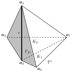
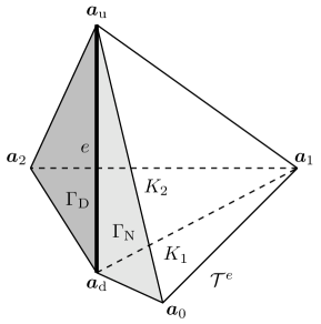
If , denotes the set of edges of , whereas for each edge , we denote by the associated “edge patch” that consists of those tetrahedra for which , see Figure 1. We also employ the notation for the open subdomain associated with the patch . We say that is a boundary edge if it lies on and that it is an interior edge otherwise (in this case, may touch the boundary at one of its endpoints). The set of boundary edges is partitioned into the subset of Dirichlet edges with edges that lie in and the subset of Neumann edges collecting the remaining boundary edges. For all edges , we denote by the open subset of corresponding to the collection of faces having as edge and lying in . Note that for interior edges, is empty and that for boundary edges, never equals the whole . We also set . Note that, in all situations, is simply connected and is connected, so that we do not need to invoke here the cohomology spaces.

For every tetrahedron , we denote the diameter and the inscribed ball diameter respectively by
where is the ball of diameter centered at . For every edge , is its measure (length) and
| (2.3) |
The shape-regularity parameters of the tetrahedron and of the edge patch are respectively defined by
| (2.4) |
2.4. Lagrange, Nédélec, and Raviart–Thomas elements
If is a tetrahedron and is an integer, we employ the notation for the space of scalar-valued (Lagrange) polynomials of degree less than or equal to on and for homogeneous polynomials of degree . The notation (resp. ) then stands for the space of vector-valued polynomials such that all their components belong to (resp. ). Following [39] and [44], we then define on each tetrahedron the polynomial spaces of Nédélec and Raviart–Thomas functions as follows:
| (2.5) |
where . For any collection of tetrahedra and the corresponding open subdomain , we also write
2.5. Nédélec finite element discretization
For the discretization of problem (2.1), we consider in this work, for a fixed polynomial degree , the Nédélec finite element space given by
The discrete counterpart of , namely
can be readily identified as a preprocessing step by introducing cuts in the mesh [42, Chapter 6]. The discrete problem then consists in finding a pair such that
| (2.6) |
Since , picking in the second equation of (2.6) shows that , so that we actually have
| (2.7) |
As for the continuous problem, we remark that when is simply connected and is connected, , where is the usual Lagrange finite element space.
3. Main results
This section presents our two main results.
3.1. Stable discrete best-approximation of broken polynomials in H
Our first main result is the combination and extension of [16, Theorem 7.2] and [10, Corollary 3.4] to the edge patches , complementing similar previous achievements in in two space dimensions in [5, Theorem 7] and in and in three space dimensions [25, Corollaries 3.1 and 3.3].
Theorem 3.1 ( best-approximation in an edge patch).
Let an edge and the associated edge patch with subdomain be fixed. Then, for every polynomial degree , all with , and all , the following holds:
| (3.1) |
Here, both minimizers are uniquely defined and the constant only depends on the shape-regularity parameter of the patch defined in (2.4).
Note that the converse inequality to (3.1) holds trivially with constant , i.e.,
This also makes apparent the power of the result (3.1), stating that for piecewise polynomial data and , the best-approximation error over a piecewise polynomial subspace of of degree is, up to a -independent constant, equivalent to the best-approximation error over the entire space . The proof of this result is presented in Section 6. We remark that Proposition 6.6 below gives an equivalent reformulation of Theorem 3.1 in the form of a stable broken polynomial extension in the edge patch. Finally, the following form, which follows from the proof in Section 6.5, see Remark 6.11, has important practical applications:
Theorem 3.2 ( best-approximation by an explicit sweep through an edge patch).
Let the assumptions of Theorem 3.1 be satisfied. Consider a sequential sweep over all elements sharing the edge , such that (i) the enumeration starts from an arbitrary tetrahedron if is an interior edge and from a tetrahedron containing a face that lies in (if any) or in (if none in ) if is a boundary edge; (ii) two consecutive tetrahedra in the enumeration share a face. On each , consider
| (3.2) |
Here, is the set of faces that shares with elements previously considered or lying in , and denotes the restriction of the tangential trace of to the faces of (see Definition 6.1 below for details). The boundary datum is either the tangential trace of obtained after minimization over the previous tetrahedron , or on . Then,
| (3.3) |
3.2. -robust broken patchwise equilibration a posteriori error estimates for the curl–curl problem
Our second main result is a polynomial-degree-robust a posteriori error analysis of Nédélec finite elements (2.6) applied to curl–curl problem (1.2). The local efficiency proof is an important application of Theorem 3.1. To present these results in detail, we need to prepare a few tools.
3.2.1. Functional inequalities and data oscillation
For every edge , we associate with the subdomain a local Sobolev space with mean/boundary value zero,
| (3.4) |
Poincaré’s inequality then states that there exists a constant only depending on the shape-regularity parameter such that
| (3.5) |
To define our error estimators, it is convenient to introduce a piecewise polynomial approximation of the datum by setting on every edge patch associated with the edge ,
| (3.6) |
This leads to the following data oscillation estimators:
| (3.7) |
where the constant is such that for every edge , we have
| (3.8) |
We show in Appendix A that only depends on the shape-regularity parameter . Notice that (3.8) is a local Poincaré-like inequality using the curl of divergence-free fields in the edge patch. This type of inequality is known under various names in the literature. Seminal contributions can be found in the work of Friedrichs [27, equation (5)] for smooth manifolds (see also Gaffney [28, equation (2)]) and later in Weber [49] for Lipschitz domains. This motivates the present use of the subscript PFW in (3.8).
Besides the above local functional inequalities, we shall also use the fact that there exists a constant such that for all , there exists such that and
| (3.9) |
When either or has zero measure, the existence of follows from Theorems 3.4 and 3.5 of [9]. If in addition is convex, one can take (see [9] together with [31, Theorem 3.7] for Dirichlet boundary conditions and [31, Theorem 3.9] for Neumann boundary conditions). For mixed boundary conditions, the existence of can be obtained as a consequence of [34, Section 2]. Indeed, we first project onto without changing its curl. Then, we define from using [34]. Finally, we control by with the inequality from [26, Proposition 7.4] which is a global Poincaré-like inequality in the spirit of (3.8).
3.2.2. Broken patchwise equilibration by edge-patch problems
Our a posteriori error estimator is constructed via a simple restriction of the right-hand side of (1.3) to edge patches, where no hat function is employed, no modification of the source term appears, and no boundary condition is imposed for interior edges, in contrast to the usual equilibration in [18, 6, 24]. For each edge , introduce
| (3.10a) | |||
| where is the argument of the left minimizer in (3.1) for the datum from (3.6) and , i.e., | |||
| (3.10b) | |||
In practice, is computed from the Euler–Lagrange conditions for the minimization problem (3.10b). This leads to the following patchwise mixed finite element problem: Find , , and such that
| (3.11) |
for all , , and . We note that from the optimality condition associated with (3.6), using or in (3.11) is equivalent.
3.2.3. Broken patchwise equilibration by sequential sweeps
The patch problems (3.10b) lead to the solution of the linear systems (3.11). Although these are local around each edge and are mutually independent, they entail some computational cost. This cost can be significantly reduced by taking inspiration from [18], [36], [48, Section 4.3.3], the proof of [5, Theorem 7], or [25, Section 6] and literally following the proof in Section 6.5 below, as summarized in Theorem 3.2. This leads to an alternative error estimator whose price is the sequential sweep through tetrahedra sharing the given edge, where for each tetrahedron, one solves the elementwise problem (3.2) for the datum from (3.6) and , i.e.,
| (3.12a) | |||
| and then set | |||
| (3.12b) | |||
3.2.4. Guaranteed, locally efficient, and -robust a posteriori error estimates
For each edge , let be the (scaled) edge basis functions of the lowest-order Nédélec space, in particular satisfying . More precisely, let be the unique function in such that
| (3.13) |
recalling that is the unit tangent vector orienting the edge . We define
| (3.14) |
where is Poincaré’s constant from (3.5) and is the diameter of the patch domain . We actually show in Lemma 5.3 below that
| (3.15) |
where is defined in (2.3); is thus uniformly bounded by the patch-regularity parameter defined in (2.4).
Theorem 3.3 (-robust a posteriori error estimate).
Let be the weak solution of the curl–curl problem (2.1) and let be its Nédélec finite element approximation solving (2.6). Let the data oscillation estimators be defined in (3.7) and the broken patchwise equilibration estimators be defined in either (3.10) or (3.12). Then, with the constants , , and from respectively (3.9), (3.14), and (3.1), the following global upper bound holds true:
| (3.16) |
as well as the following lower bound local to the edge patches :
| (3.17) |
3.3. Comments
A few comments about Theorem 3.3 are in order.
-
•
The constant from (3.9) can be taken as for convex domains and if either or is empty. In the general case however, we do not know the value of this constant. The presence of the constant is customary in a posteriori error analysis of the curl–curl problem, it appears, e.g., in Lemma 3.10 of [41] and Assumption 2 of [2].
-
•
The constant defined in (3.14) can be fully computed in practical implementations. Indeed, computable values of Poincaré’s constant from (3.5) are discussed in, e.g., [8, 47], see also the concise discussion in [3]; can be taken as for convex interior patches and as for most Dirichlet boundary patches. Recall also that only depends on the shape-regularity parameter of the edge patch .
- •
- •
-
•
In contrast to [6, 29, 30, 35], we do not obtain here an equilibrated flux, i.e., a piecewise polynomial in the global space satisfying, for piecewise polynomial , . We only obtain from (3.10b) or (3.12a) that and locally in every edge patch and similarly for , but we do not build a -conforming discrete field; we call this process broken patchwise equilibration.
-
•
The upper bound (3.16) does not come from the Prager–Synge inequality (1.3) and is typically larger than those obtained from (1.3) with an equilibrated flux , because of the presence of the multiplicative factors . On the other hand, it is typically cheaper to compute the upper bound (3.16) than those based on an equilibrated flux since 1) the problems (3.10) and (3.12) involve edge patches, whereas full equilibration would require solving problems also on vertex patches which are larger than edge patches; 2) the error estimators are computed in one stage only solving the problems (3.10b) or (3.12a); 3) the broken patchwise equilibration procedure enables the construction of a -robust error estimator using polynomials of degree , in contrast to the usual procedure requiring the use of polynomials of degree , cf. [5, 24, 25]; the reason is that the usual procedure involves multiplication by the “hat function” inside the estimators, which increases the polynomial degree by one, whereas the current procedure only encapsulates an operation featuring into the multiplicative constant , see (3.14).
-
•
The sequential sweep through the patch in (3.12a) eliminates the patchwise problems (3.10b) and leads instead to merely elementwise problems. These are much cheaper than (3.10b), and, in particular, for , i.e., for lowest-order Nédélec elements in (2.6) with one unknown per edge, they can be made explicit. Indeed, there is only one unknown in (3.12a) for each tetrahedron if is not the first or the last tetrahedron in the sweep. In the last tetrahedron, there is no unknown left except if it contains a face that lies in , in which case there is also only one unknown in (3.12a). If the first tetrahedron contains a face that lies in , there is again only one unknown in (3.12a). Finally, if the first tetrahedron does not contain a face that lies in , it is possible, instead of , to consider the set formed by the face that either 1) lies in (if any) or 2) is shared with the last element and to employ for the boundary datum in (3.12a) the 1) value or 2) the mean value of the tangential trace on . This again leads to only one unknown in (3.12a), with all the theoretical properties maintained.
4. Numerical experiments
In this section, we present some numerical experiments to illustrate the a posteriori error estimates from Theorem 3.3 and its use within an adaptive mesh refinement procedure. We consider a test case with a smooth solution and a test case with a solution featuring an edge singularity.
Below, we rely on the indicator evaluated using (3.10), i.e., involving the edge-patch solves (3.11). Moreover, we let
| (4.1) |
Here, corresponds to an “oscillation-free” error estimator, obtained by discarding the oscillation terms in (3.16), whereas corresponds to a “constant-and-oscillation-free” error estimator, discarding in addition the multiplicative constants and .
4.1. Smooth solution in the unit cube
We first consider an example in the unit cube and Neumann boundary conditions, in (1.2) and its weak form (2.1). The analytical solution reads
One checks that and that
We notice that since is convex.
We first propose an “-convergence” test case in which, for a fixed polynomial degree , we study the behavior of the Nédélec approximation solving (2.6) and of the error estimator of Theorem 3.3. We consider a sequence of meshes obtained by first splitting the unit cube into an Cartesian grid and then splitting each of the small cubes into six tetrahedra, with the resulting mesh size . More precisely, each resulting edge patch is convex here, so that the constant in (3.14) can be taken as for all internal patches, see the discussion in Section 3.2.1. Figure 2 presents the results. The top-left panel shows that the expected convergence rates of are obtained for . The top-right panel presents the local efficiency of the error estimator based on the indicator evaluated using (3.10). We see that it is very good, the ratio of the patch indicator to the patch error being at most for , and close to for higher-order polynomials. This seems to indicate that the constant in (3.1) is rather small. The bottom panels of Figure 2 report on the global efficiency of the error indicators and from (4.1). As shown in the bottom-right panel, the global efficiency of is independent of the mesh size. The bottom-left panel shows a slight dependency of the global efficiency of on the mesh size, but this is only due to the fact that Poincaré’s constants differ for boundary and internal patches. These two panels show that the efficiency actually slightly improves as the polynomial degree is increased, highlighting the -robustness of the proposed error estimator. We also notice that the multiplicative factor can lead to some error overestimation.
We then present a “-convergence” test case where for a fixed mesh, we study the behavior of the solution and of the error estimator when the polynomial degree is increased. We provide this analysis for four different meshes. The three first meshes are structured as previously described with , and , whereas the last mesh is unstructured. The unstructured mesh has elements, edges, and . Figure 3 presents the results. The top-left panel shows an exponential convergence rate as is increased for all the meshes, which is in agreement with the theory, since the solution is analytic. The top-right panel shows that the local patch-by-patch efficiency is very good, and seems to tend to as increases. The bottom-right panel shows that the global efficiency of also slightly improves as is increased, and it seems to be rather independent of the mesh. The bottom-left panel shows that the global efficiency of is significantly worse on the unstructured mesh. This is because in the absence of convex patches, we employ for the estimate from [47] instead of the constant . We believe that this performance could be improved by providing sharper Poincaré constants.
4.2. Singular solution in an L-shaped domain
We now turn our attention to an L-shaped domain featuring a singular solution. Specifically, , where
see Figure 5, where is represented. We consider the case , and the solution reads , where , , , and is a smooth cutoff function such that in a neighborhood of . We emphasize that and that, since near the origin, the right-hand side associated with belongs to .
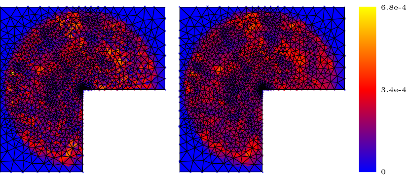
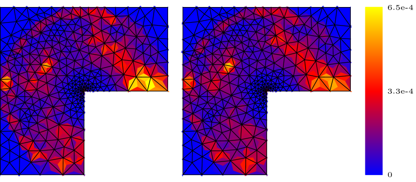
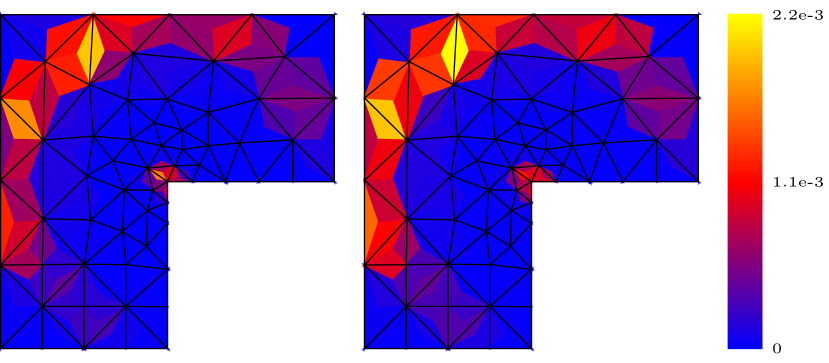
We use an adaptive mesh-refinement strategy based on Dörfler’s marking [20]. The initial mesh we employ for and consists of elements and edges with , whereas a mesh with elements, edges, and is employed for and . The meshing package MMG3D is employed to generate the sequence of adapted meshes [19]. Figure 4 shows the convergence histories of the adaptive algorithm for different values of . In the top-left panel, we observe the optimal convergence rate (limited to for isotropic elements in the presence of an edge singularity). We employ the indicator defined in (4.1). The top-right and bottom-left panels respectively present the local and global efficiency indices. In both cases, the efficiency is good considering that the mesh is fully unstructured with localized features. We also emphasize that the efficiency does not deteriorate when increases.
Finally, Figure 5 depicts the estimated and the actual errors at the last iteration of the adaptive algorithm. The face on the top of the domain is represented, and the colors are associated with the edges of the mesh. The left panels correspond to the values of the estimator of (3.10), whereas the value of is represented in the right panels. Overall, this figure shows excellent agreement between the estimated and actual error distribution.
5. Proof of Theorem 3.3 (-robust a posteriori error estimate)
In this section, we prove Theorem 3.3.
5.1. Residuals
Recall that solves (2.6) and satisfies (2.7). In view of the characterization of the weak solution (2.2), we define the residual by setting
Taking and using a duality characterization, we have the error–residual link
| (5.1) |
We will also employ local dual norms of the residual . Specifically, for each edge , we set
| (5.2) |
For each , we will also need an oscillation-free residual defined using the projected right-hand side introduced in (3.6),
We also employ the notation
for the dual norm of . Note that whenever the source term is a piecewise polynomial.
5.2. Data oscillation
Recalling the definition (3.7) of , we have the following comparison:
Lemma 5.1 (Data oscillation).
The following holds true:
| (5.3a) | |||
| and | |||
| (5.3b) | |||
5.3. Partition of unity and cut-off estimates
We now analyze a partition of unity for vector-valued functions that we later employ to localize the error onto edge patches. Recalling the notation for the unit tangent vector orienting , we quote the following classical partition of unity [22, Chapter 15]:
Lemma 5.2 (Vectorial partition of unity).
Let be the identity matrix in . The edge basis functions from (3.13) satisfy
where denotes the outer product, so that we have
| (5.4) |
Lemma 5.3 (Cut-off stability).
Proof.
Let an edge and be fixed. Since , we have, using (3.5),
This proves (5.5). To prove (3.15), we remark that in every tetrahedron , we have (see for instance [37, Section 5.5.1], [22, Chapter 15])
where and are the barycentric coordinates of associated with the two endpoints of such that points from the first to the second vertex. Since and , we have
for every . Recalling the definition (2.3) of , which implies that , as well as the definition in (2.4), we conclude that
∎
5.4. Upper bound using localized residual dual norms
We now establish an upper bound on the error using the localized residual dual norms , in the spirit of [3], [23, Chapter 34], and the references therein.
Proposition 5.4 (Upper bound by localized residual dual norms).
Proof.
We start with (6.26). Let with be fixed. Following (3.9), we define such that with
| (5.7) |
As a consequence of (2.2) and (2.7), the residual is (in particular) orthogonal to . Thus, by employing the partition of unity (5.4), we have
where if and
otherwise. Since for all , we have from (5.2)
We observe that for all and that
As a result, (5.5) shows that
At this point, as each tetrahedron has edges, we have
and using (5.7), we infer that
Then, we conclude with (5.3b). ∎
5.5. Lower bound using localized residual dual norms
We now consider the derivation of local lower bounds on the error using the residual dual norms. We first establish a result for the residual .
Lemma 5.5 (Local residual).
For every edge , the following holds:
| (5.8) |
as well as
| (5.9) |
Proof.
Let us define as the unique element of such that
| (5.10) |
The existence and uniqueness of follows from [26, Proposition 7.4] after lifting by .
We are now ready to state our results for the oscillation-free residuals .
Lemma 5.6 (Local oscillation-free residual).
For every edge , the following holds:
| (5.11) |
as well as
| (5.12) |
5.6. Proof of Theorem 3.3
We are now ready to give a proof of Theorem 3.3.
On the one hand, the broken patchwise equilibration estimator defined in (3.10) is evaluated from a field such that , and the sequential sweep (3.12) produces also satisfying these two properties. Since the minimization set in (5.11) is larger, it is clear that
for both estimators . Then, (3.16) immediately follows from (5.6).
6. Equivalent reformulation and proof of Theorem 3.1 ( best-approximation in an edge patch)
In this section, we consider the minimization problem over an edge patch as posed in the statement of Theorem 3.1, as well as its sweep variant of Theorem 3.2, which were central tools to establish the efficiency of the broken patchwise equilibrated error estimators in Theorem 3.3. These minimization problems are similar to the ones considered in [5, 24, 25] in the framework of and spaces. We prove here Theorem 3.1 via its equivalence with a stable broken polynomial extension on an edge patch, as formulated in Proposition 6.6 below. By virtue of Remark 6.11, this also establishes the validity of Theorem 3.2.
6.1. Stability of discrete minimization in a tetrahedron
6.1.1. Preliminaries
We first recall some necessary notation from [7]. Consider an arbitrary mesh face oriented by the fixed unit vector normal . For all , we define the tangential component of as
| (6.1) |
Note that the orientation of is not important here. Let and let be the collection of the faces of . For all and all , the tangential trace of on is defined (with a slight abuse of notation) as .
Consider now a nonempty subset . We denote the corresponding part of the boundary of . Let be the polynomial degree and recall that is the Nédélec space on the tetrahedron , see (2.5). We define the piecewise polynomial space on
| (6.2) |
Note that if and only if for all and whenever , for every pair of distinct faces in , the following tangential trace compatibility condition holds true along their common edge :
| (6.3) |
For all , we set
| (6.4) |
which is well-defined independently of the choice of . Note that the orientation of is relevant here.
The definition (6.1) of the tangential trace cannot be applied to fields with the minimal regularity . In what follows, we use the following notion to prescribe the tangential trace of a field in .
Definition 6.1 (Tangential trace by integration by parts in a single tetrahedron).
Let be a tetrahedron and a nonempty (sub)set of its faces. Given and , we employ the notation “” to say that
where
Whenever , if and only if for all .
6.1.2. Statement of the stability result in a tetrahedron
Recall the Raviart–Thomas space on the simplex , see (2.5). We are now ready to state a key technical tool from [7, Theorem 2], based on [16, Theorem 7.2] and [10, Proposition 4.2].
Proposition 6.2 (Stable polynomial extension on a tetrahedron).
Let be a tetrahedron and let be a (sub)set of its faces. Then, for every polynomial degree , for all such that , and if , for all such that for all , the following holds:
| (6.5) |
where the condition on the tangential trace in the minimizing sets is null if . Both minimizers in (6.5) are uniquely defined and the constant only depends on the shape-regularity parameter of .
6.2. Piola mappings
This short section reviews some useful properties of Piola mappings used below, see [22, Chapter 9]. Consider two tetrahedra and an invertible affine mapping such that . Let be the (constant) Jacobian matrix of . Note that we do not require that is positive. The affine mapping can be identified by specifying the image of each vertex of . We consider the covariant and contravariant Piola mappings
for vector-valued fields . It is well-known that maps onto and it maps onto for any polynomial degree . Similarly, maps onto and it maps onto . Moreover, the Piola mappings and commute with the curl operator in the sense that
| (6.6) |
In addition, we have
| (6.7) |
for all and . We also have for all , so that whenever belong to the same edge patch , we have
| (6.8) |
for a constant only depending on the shape-regularity of the patch defined in (2.4).
6.3. Stability of discrete minimization in an edge patch
6.3.1. Preliminaries
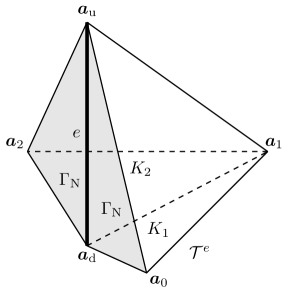
In this section, we consider an edge patch associated with a mesh edge consisting of tetrahedral elements sharing the edge , cf. Figure 1. We denote by the number of tetrahedra in the patch, by the set of all faces of the patch, by the set of “internal” faces, i.e., those being shared by two different tetrahedra from the patch, and finally, by the set of “external” faces. The patch is either of “interior” type, corresponding to an edge in the interior of the domain , in which case there is a full loop around , see Figure 1, left, or of “boundary” type, corresponding to an edge on the boundary of the domain , in which case there is no full loop around , see Figure 1, right, and Figure 6. We further distinguish three types of patches of boundary type depending on the status of the two boundary faces sharing the associated boundary edge: the patch is of Dirichlet boundary type if both faces lie in , of “mixed boundary” type if one face lies in an the other in , and of Neumann boundary type if both faces lie in . Note that for an interior patch, , whereas for a boundary patch. The open domain associated with is denoted by , and stands for the unit normal vector to pointing outward .
We denote by and the two vertices of the edge . The remaining vertices are numbered consecutively in one sense of rotation around the edge (this sense is only specific for the “mixed boundary” patches) and denoted by , with if the patch is interior. Then for ; we also denote and . For all , we define , and for all , we let and . Then , and if the patch is interior. We observe that, respectively for interior and boundary patches, , and , . Finally, if is an internal face, we define its normal vector by , whereas for any external face , we define its normal vector to coincide with the normal vector pointing outward the patch, .
We now extend the notions of Section 6.1.1 to the edge patch . Consider the following broken Sobolev spaces:
as well as the broken Nédélec space . For all , we employ the notation for the “(strong) jump” of across any face . Specifically, for an internal face , we set , whereas for an external face , we set . Note in particular that piecewise polynomial functions from belong to , so that their strong jumps are well-defined.
To define a notion of a “weak tangential jump” for functions of , for which a strong (pointwise) definition cannot apply, some preparation is necessary. Let be a subset of the faces of an edge patch containing the internal faces, i.e. , and denote by the corresponding open set. The set represents the set of faces appearing in the minimization. It depends on the type of edge patch and is reported in Table 1. In extension of (6.2), we define the piecewise polynomial space on
| (6.9) |
In extension of (6.4), for all , we set
| (6.10) |
Then we can extend Definition 6.1 to prescribe weak tangential jumps of functions in as follows:
| patch type | ||
|---|---|---|
| interior | ||
| Dirichlet boundary | ||
| mixed boundary | ||
| Neumann boundary |
Definition 6.3 (Tangential jumps by integration by parts in an edge patch).
Given and , we employ the notation “” to say that
| (6.11) |
where
| (6.12) |
Whenever , if and only if for all . Note that in (6.11) is uniquely defined for all .
6.3.2. Statement of the stability result in an edge patch
Henceforth, if is an elementwise Raviart–Thomas function, we will employ the notation for all . In addition, if is an elementwise Nédélec function, the notations and will be understood elementwise.
Definition 6.4 (Compatible data).
Let and . We say that the data and are compatible if
| (6.13a) | ||||||
| (6.13b) | ||||||
| and with the following additional condition whenever the patch is either of interior or Neumann boundary type: | ||||||
| (6.13c) | ||||||
| (6.13d) | ||||||
Definition 6.5 (Broken patch spaces).
Let and be compatible data as per Definition 6.4. We define
| (6.14c) | ||||
| (6.14d) | ||||
We will show in Lemma 6.10 below that the space (and therefore also ) is nonempty. We are now ready to present our central result of independent interest. To facilitate the reading, the proof is postponed to Section 6.5.
Proposition 6.6 (Stable broken polynomial extension in an edge patch).
Let an edge and the associated edge patch with subdomain be fixed. Let the set of faces be specified in Table 1. Then, for every polynomial degree , all , and all compatible as per Definition 6.4, the following holds:
| (6.15) |
Here, all the minimizers are uniquely defined and the constant only depends on the shape-regularity parameter of the patch defined in (2.4).
6.4. Equivalence of Theorem 3.1 with Proposition 6.6
We have the following important link, establishing Theorem 3.1, including the existence and uniqueness of the minimizers.
Lemma 6.8 (Equivalence of Theorem 3.1 with Proposition 6.6).
Theorem 3.1 holds if and only if Proposition 6.6 holds. More precisely, let and by any solutions to the minimization problems of Theorem 3.1 for the data with and . Let and be any minimizers of Proposition 6.6 for the data
| (6.16) |
where is specified in Table 1. Then
| (6.17) |
In the converse direction, for given data and in Proposition 6.6, compatible as per Definition 6.4, taking any such that for all and gives minimizers of Theorem 3.1 such that (6.17) holds true.
Proof.
The proof follows via a shift by the datum . In order to show (6.17) in the forward direction (the converse direction is actually easier), we merely need to show that and prescribed by (6.16) are compatible data as per Definition 6.4. Indeed, to start with, since , we have . In addition, since from (3.6),
which is (6.13a). Then, for all if the patch is of interior type and for all if the patch is of boundary type, we have
and therefore, recalling the definition (6.4) of the surface curl, we infer that
On the other hand, since , we have , and therefore
Since a similar reasoning applies on the face if the patch is of Neumann or mixed boundary type and on the face if the patch is of Neumann boundary type, (6.13b) is established.
It remains to show that satisfies the edge compatibility condition (6.13c) or (6.13d) if the patch is interior or Neumann boundary type, respectively. Let us treat the first case (the other case is treated similarly). Owing to the convention , we infer that
which establishes (6.13c). We have thus shown that and are compatible data as per Definition 6.4. ∎
6.5. Proof of Proposition 6.6
The proof of Proposition 6.6 is performed in two steps. First we prove that is nonempty by providing a generic elementwise construction of a field in ; this in particular implies the existence and uniqueness of all minimizers in (6.15). Then we prove the inequality (6.15) by using one such field . Throughout this section, if are two real numbers, we employ the notation to say that there exists a constant that only depends on the shape-regularity parameter of the patch defined in (2.4), such that . We note that in particular we have owing to the shape-regularity of the mesh .
6.5.1. Generic elementwise construction of fields in
The generic construction of fields in is based on a loop over the mesh elements composing the edge patch . This loop is enumerated by means of an index .
Definition 6.9 (Element spaces).
For each , let be a (sub)set of the faces of . Let with , and if , let in the sense of (6.2) be given data. We define
| (6.18c) | ||||
| (6.18d) | ||||
In what follows, we are only concerned with the cases where is either empty or composed of one or two faces of . In this situation, the subspace is nonempty if and only if
| (6.19a) | |||||
| (6.19b) | |||||
where is the unit normal orienting used in the definition of the surface curl (see (6.4)). The second condition (6.19b) is relevant only if .
Lemma 6.10 (Generic elementwise construction).
Let , let be the edge patch associated with , and let
the set of faces be specified in Table 1.
Let and be compatible data
as per Definition 6.4. Define
for all . Then,
the following inductive procedure yields a sequence of nonempty spaces
in the sense of Definition 6.9,
as well as a sequence of fields
such that for all . Moreover, the field
prescribed by for all belongs to the space
of Definition 6.5:
| 1) First element (): Set if the patch is of interior or Dirichlet boundary type and set if the patch is of Neumann or mixed boundary type together with | ||||||
| (6.20a) | ||||||
|
Define the space according to (6.18d) and pick any
.
2) Middle elements (): Set together with | ||||||
| (6.20b) | ||||||
|
with obtained in the previous step of the procedure.
Define the space according to (6.18d) and pick any
.
3) Last element (): Set if the patch is of Dirichlet or mixed boundary type and set if the patch is of interior or Neumann boundary type and define as follows: For the four cases of the patch, | ||||||
| (6.20c) | ||||||
| with obtained in the previous step of the procedure, and in the two cases where also contains : | ||||||
| (6.20d) | ||||||
| (6.20e) | ||||||
|
Define the space according to (6.18d) and pick any
.
| ||||||
Proof.
We first show that is well-defined in for all . We do so by verifying that (recall (6.2)) and that the conditions (6.19) hold true for all . Then, we show that .
(1) First element (). If the patch is of interior or Dirichlet boundary type, there is nothing to verify since is empty. If the patch is of Neumann or mixed boundary type, and we need to verify that and that , see (6.19a). Since by assumption, the first requirement is met. The second one follows from owing to (6.13b).
(2) Middle elements (). Since , we need to show that and that . The first requirement follows from the definition (6.20b) of . To verify the second requirement, we recall the definition (6.4) of the surface curl and use the curl constraint from (6.18c) to infer that
By virtue of assumption (6.13b), it follows that
(3) Last element (). We distinguish two cases.
(3a) Patch of Dirichlet or mixed boundary type. In this case, and the reasoning is identical to the case of a middle element.
(3b) Patch of interior or Neumann boundary type. In this case, . First, the prescriptions (6.20c)–(6.20d)–(6.20e) imply that in the sense of (6.2). It remains to show (6.19a), i.e.
| (6.21) |
and, since is composed of two faces, we also need to show the edge compatibility condition (6.19b), i.e.
| (6.22) |
The proof of the first identity in (6.21) is as above, so we now detail the proof of the second identity in (6.21) and the proof of (6.22).
(3b-I) Let us consider the case of a patch of interior type. To prove the second identity in (6.21), we use definition (6.4) of the surface curl together with the curl constraint in (6.18c) and infer that
This gives
where the last equality follows from (6.13b). This proves the expected identity on the curl.
Let us now prove (6.22). For all , since , its tangential traces satisfy the edge compatibility condition
| (6.23) |
Moreover, for all , we have , so that by (6.18c) and the definition (6.20b) of , we have
and, therefore, using (6.23) yields
Summing this identity for all leads to
In addition, using again the edge compatibility condition (6.23) for and the definition (6.20c) of leads to
Summing the above two identities gives
| (6.24) |
Since for a patch of interior type and owing to (6.20d), the identity (6.24) gives
where we used the edge compatibility condition (6.13c) satisfied by in the last equality. This proves (6.22) in the interior case.
(3b-N) Let us finally consider a patch of Neumann boundary type. The second identity in (6.21) follows directly from (6.13b) and (6.20e). Let us now prove (6.22). The identity (6.24) still holds true. Using that , this identity is rewritten as
where the last equality follows from the edge compatibility condition (6.13d) satisfied by . But since owing to (6.20e), this again proves (6.22).
6.5.2. The actual proof
We are now ready to prove Proposition 6.6.
Proof of Proposition 6.6.
Owing to Lemma 6.10, the fields
| (6.25) |
are uniquely defined in , and the field such that for all satisfies . Since the minimizing sets in (6.15) are nonempty (they all contain ), both the discrete and the continuous minimizers are uniquely defined owing to standard convexity arguments. Let us set
To prove Proposition 6.6, it is enough to show that
| (6.26) |
Owing to Proposition 6.2 applied with and for all , we have
| (6.27) |
where is defined in (6.18c). Therefore, recalling that , (6.26) will be proved if for all , we can construct a field such that . To do so, we proceed once again by induction.
(1) First element (). Since , the claim is established with which trivially satisfies .
(2) Middle elements (). We proceed by induction. Given such that , let us construct a suitable such that . We consider the affine geometric mapping that leaves the three vertices , , and (and consequently the face ) invariant, whereas . We denote by the associated Piola mapping, see Section 6.2. Let us define the function by
| (6.28) |
where (notice that here ). Using the triangle inequality, the -stability of the Piola mapping (see (6.8)), inequality (6.27), and the induction hypothesis, we have
| (6.29) |
Thus it remains to establish that in the sense of Definition 6.9, i.e., we need to show that and . Recalling the curl constraints in (6.14c) and (6.18c) which yield and using (6.6), we have
| (6.30) |
which proves the expected condition on the curl of .
It remains to verify the weak tangential trace condition as per Definition 6.1. To this purpose, let and define by
| (6.31) |
These definitions imply that (recall (6.12)) with
as well as
(Note that is uniquely defined by assumption.) Recalling definition (6.28) of and that , see (6.30), we have
where we used the definition of , properties (6.7), (6.6) of the Piola mapping, and the definition of to infer that
Since and outside , this gives
| (6.32) | ||||
Since , , and , we have from Definitions 6.3 and 6.5
| (6.33) | ||||
where in the last equality, we employed the definition (6.31) of . On the other hand, since , we can employ the pointwise definition of the trace and infer that
| (6.34) | ||||
where we used that . Then, plugging (6.33) and (6.34) into (6.32) and employing (6.20b) and , we obtain
Since , this shows that satisfies the weak tangential trace condition in by virtue of Definition 6.1.
(3) Last element (). We need to distinguish the type of patch.
(3a) Patch of Dirichlet or mixed boundary type. In this case, we can employ the same argument as for the middle elements since is composed of only one face.
(3b) Patch of interior type. Owing to the induction hypothesis, we have for all . Let us first assume that there is an even number of tetrahedra in the patch , as in Figure 1, left. The case where this number is odd will be discussed below. We build a geometric mapping for all as follows: leaves the edge pointwise invariant, , if is odd, and , if is even. Since is by assumption even, one readily sees that with for all .
We define by setting
| (6.35) |
where and is the Piola mapping associated with . Reasoning as above in (6.29) shows that
It now remains to establish that as per Definition 6.9, i.e. and with . Since , using (6.6) leads to as above in (6.30), which proves the expected condition on the curl of . It remains to verify the weak tangential trace condition as per Definition 6.1. To this purpose, let and define by
| (6.36) |
As , its trace is defined in a strong sense, and the preservation of tangential traces by Piola mappings shows that in the sense of (6.12). Then, using and (6.35), we have
where we used the definition of for the first two terms on the right-hand side. Moreover, using (6.7) and (6.6) for all , we have
since . It follows that
where we employed the fact that, since both , Definition 6.3 gives
Thus in the sense of Definition 6.1. This establishes the weak tangential trace condition on when is even.
If is odd, one can proceed as in [25, Section 6.3]. For the purpose of the proof only, one tetrahedron different from is subdivided into two subtetrahedra as in [25, Lemma B.2]. Then, the above construction of can be applied on the newly created patch which has an even number of elements, and one verifies as above that .
(3c) Patch of Neumann boundary type. In this case, a similar argument as for a patch of interior type applies, and we omit the proof for the sake of brevity.
∎
Remark 6.11 (Quasi-optimality of ).
References
- [1] Franck Assous, Patrick Ciarlet, Jr., and Simon Labrunie, Mathematical foundations of computational electromagnetism, Applied Mathematical Sciences, vol. 198, Springer, Cham, 2018. MR 3793186
- [2] Rudi Beck, Ralf Hiptmair, Ronald H. W. Hoppe, and Barbara Wohlmuth, Residual based a posteriori error estimators for eddy current computation, M2AN Math. Model. Numer. Anal. 34 (2000), no. 1, 159–182. MR 1735971
- [3] Jan Blechta, Josef Málek, and Martin Vohralík, Localization of the norm for local a posteriori efficiency, IMA J. Numer. Anal. 40 (2020), no. 2, 914–950.
- [4] Alain Bossavit, Computational electromagnetism, Electromagnetism, Academic Press, Inc., San Diego, CA, 1998, Variational formulations, complementarity, edge elements. MR 1488417
- [5] Dietrich Braess, Veronika Pillwein, and Joachim Schöberl, Equilibrated residual error estimates are -robust, Comput. Methods Appl. Mech. Engrg. 198 (2009), no. 13-14, 1189–1197. MR 2500243
- [6] Dietrich Braess and Joachim Schöberl, Equilibrated residual error estimator for edge elements, Math. Comp. 77 (2008), no. 262, 651–672. MR 2373174 (2008m:65313)
- [7] Théophile Chaumont-Frelet, Alexandre Ern, and Martin Vohralík, Polynomial-degree-robust -stability of discrete minimization in a tetrahedron, C. R. Math. Acad. Sci. Paris 358 (2020), no. 9–10, 1101–1110.
- [8] Seng-Kee Chua and Richard L. Wheeden, Estimates of best constants for weighted Poincaré inequalities on convex domains, Proc. London Math. Soc. (3) 93 (2006), no. 1, 197–226. MR MR2235947 (2006m:26030)
- [9] Martin Costabel, Monique Dauge, and Serge Nicaise, Singularities of Maxwell interface problems, M2AN Math. Model. Numer. Anal. 33 (1999), no. 3, 627–649. MR 1713241
- [10] Martin Costabel and Alan McIntosh, On Bogovskiĭ and regularized Poincaré integral operators for de Rham complexes on Lipschitz domains, Math. Z. 265 (2010), no. 2, 297–320. MR 2609313 (2011f:58030)
- [11] E. Creusé, Y. Le Menach, S. Nicaise, F. Piriou, and R. Tittarelli, Two guaranteed equilibrated error estimators for harmonic formulations in eddy current problems, Comput. Math. Appl. 77 (2019), no. 6, 1549–1562. MR 3926828
- [12] Emmanuel Creusé, Serge Nicaise, and Roberta Tittarelli, A guaranteed equilibrated error estimator for the and magnetodynamic harmonic formulations of the Maxwell system, IMA J. Numer. Anal. 37 (2017), no. 2, 750–773. MR 3649425
- [13] Patrik Daniel, Alexandre Ern, Iain Smears, and Martin Vohralík, An adaptive -refinement strategy with computable guaranteed bound on the error reduction factor, Comput. Math. Appl. 76 (2018), no. 5, 967–983.
- [14] Leszek Demkowicz, Computing with -adaptive finite elements. Vol. 1, Chapman & Hall/CRC Applied Mathematics and Nonlinear Science Series, Chapman & Hall/CRC, Boca Raton, FL, 2007, One and two dimensional elliptic and Maxwell problems, With 1 CD-ROM (UNIX). MR 2267112
- [15] Leszek Demkowicz, Jayadeep Gopalakrishnan, and Joachim Schöberl, Polynomial extension operators. Part I, SIAM J. Numer. Anal. 46 (2008), no. 6, 3006–3031. MR 2439500 (2009j:46080)
- [16] by same author, Polynomial extension operators. Part II, SIAM J. Numer. Anal. 47 (2009), no. 5, 3293–3324. MR 2551195 (2010h:46043)
- [17] by same author, Polynomial extension operators. Part III, Math. Comp. 81 (2012), no. 279, 1289–1326. MR 2904580
- [18] Philippe Destuynder and Brigitte Métivet, Explicit error bounds in a conforming finite element method, Math. Comp. 68 (1999), no. 228, 1379–1396. MR 1648383 (99m:65211)
- [19] C. Dobrzynski, MMG3D: User guide, Tech. Report 422, Inria, France, 2012.
- [20] Willy Dörfler, A convergent adaptive algorithm for Poisson’s equation, SIAM J. Numer. Anal. 33 (1996), no. 3, 1106–1124. MR 1393904 (97e:65139)
- [21] Alexandre Ern, Thirupathi Gudi, Iain Smears, and Martin Vohralík, Equivalence of local- and global-best approximations, a simple stable local commuting projector, and optimal approximation estimates in , IMA J. Numer. Anal. (2021), DOI 10.1093/imanum/draa103.
- [22] Alexandre Ern and Jean-Luc Guermond, Finite Elements I. Approximation and Interpolation, Texts in Applied Mathematics, vol. 72, Springer International Publishing, Springer Nature Switzerland AG, 2021.
- [23] by same author, Finite Elements II. Galerkin Approximation, Elliptic and Mixed PDEs, Springer International Publishing, Springer Nature Switzerland AG, 2021.
- [24] Alexandre Ern and Martin Vohralík, Polynomial-degree-robust a posteriori estimates in a unified setting for conforming, nonconforming, discontinuous Galerkin, and mixed discretizations, SIAM J. Numer. Anal. 53 (2015), no. 2, 1058–1081. MR 3335498
- [25] by same author, Stable broken and polynomial extensions for polynomial-degree-robust potential and flux reconstruction in three space dimensions, Math. Comp. 89 (2020), no. 322, 551–594.
- [26] Paolo Fernandes and Gianni Gilardi, Magnetostatic and electrostatic problems in inhomogeneous anisotropic media with irregular boundary and mixed boundary conditions, Math. Models Methods Appl. Sci. 7 (1997), no. 7, 957–991. MR 1479578
- [27] K. O. Friedrichs, Differential forms on Riemannian manifolds, Comm. Pure Appl. Math. 8 (1955), 551–590.
- [28] M. P. Gaffney, Hilbert space methods in the theory of harmonic integrals, Trans. Amer. Math. Soc. 78 (1955), 426–444.
- [29] Joscha Gedicke, Sjoerd Geevers, and Ilaria Perugia, An equilibrated a posteriori error estimator for arbitrary-order Nédélec elements for magnetostatic problems, J. Sci. Comput. 83 (2020), no. 3, Paper No. 58, 23. MR 4110650
- [30] Joscha Gedicke, Sjoerd Geevers, Ilaria Perugia, and Joachim Schöberl, A polynomial-degree-robust a posteriori error estimator for Nédélec discretizations of magnetostatic problems, arXiv preprint 2004.08323, 2020.
- [31] Vivette Girault and Pierre-Arnaud Raviart, Finite element methods for Navier-Stokes equations, Springer Series in Computational Mathematics, vol. 5, Springer-Verlag, Berlin, 1986, Theory and algorithms. MR MR851383 (88b:65129)
- [32] A. Hannukainen, Functional type a posteriori error estimates for Maxwell’s equations, Numerical mathematics and advanced applications, Springer, Berlin, 2008, pp. 41–48. MR 3615865
- [33] R. Hiptmair, Finite elements in computational electromagnetism, Acta Numerica 11 (2002), 237–339.
- [34] Ralf Hiptmair and Clemens Pechstein, Discrete regular decompositions of tetrahedral discrete 1-forms, ch. 7, pp. 199–258, De Gruyter, 2019.
- [35] Martin W. Licht, Higher-order finite element de Rham complexes, partially localized flux reconstructions, and applications, Preprint, 2019.
- [36] Robert Luce and Barbara I. Wohlmuth, A local a posteriori error estimator based on equilibrated fluxes, SIAM J. Numer. Anal. 42 (2004), no. 4, 1394–1414. MR 2114283 (2006d:65122)
- [37] Peter Monk, Finite element methods for Maxwell’s equations, Numerical Mathematics and Scientific Computation, Oxford University Press, New York, 2003. MR 2059447
- [38] Rafael Muñoz Sola, Polynomial liftings on a tetrahedron and applications to the - version of the finite element method in three dimensions, SIAM J. Numer. Anal. 34 (1997), no. 1, 282–314. MR 1445738
- [39] Jean-Claude Nédélec, Mixed finite elements in , Numer. Math. 35 (1980), no. 3, 315–341. MR MR592160 (81k:65125)
- [40] Pekka Neittaanmäki and Sergey Repin, Guaranteed error bounds for conforming approximations of a Maxwell type problem, Applied and numerical partial differential equations, Comput. Methods Appl. Sci., vol. 15, Springer, New York, 2010, pp. 199–211. MR 2642690
- [41] S. Nicaise and E. Creusé, A posteriori error estimation for the heterogeneous Maxwell equations on isotropic and anisotropic meshes, Calcolo 40 (2003), no. 4, 249–271. MR 2025712
- [42] P. Robert Kotiuga Paul W. Gross, Electromagnetic theory and computation: a topological approach, MSRI 48, Cambridge University Press, 2004.
- [43] William Prager and John L. Synge, Approximations in elasticity based on the concept of function space, Quart. Appl. Math. 5 (1947), 241–269. MR MR0025902 (10,81b)
- [44] Pierre-Arnaud Raviart and Jean-Marie Thomas, A mixed finite element method for 2nd order elliptic problems, Mathematical aspects of finite element methods (Proc. Conf., Consiglio Naz. delle Ricerche (C.N.R.), Rome, 1975), Springer, Berlin, 1977, pp. 292–315. Lecture Notes in Math., Vol. 606. MR MR0483555 (58 #3547)
- [45] S. Repin, Functional a posteriori estimates for Maxwell’s equation, J. Math. Sci. (N.Y.) 142 (2007), no. 1, 1821–1827, Problems in mathematical analysis. No. 34. MR 2331641
- [46] Ch. Schwab, - and -finite element methods, Numerical Mathematics and Scientific Computation, The Clarendon Press, Oxford University Press, New York, 1998, Theory and applications in solid and fluid mechanics. MR 1695813
- [47] Andreas Veeser and Rüdiger Verfürth, Poincaré constants for finite element stars, IMA J. Numer. Anal. 32 (2012), no. 1, 30–47. MR 2875242 (2012m:65444)
- [48] Martin Vohralík, Guaranteed and fully robust a posteriori error estimates for conforming discretizations of diffusion problems with discontinuous coefficients, J. Sci. Comput. 46 (2011), no. 3, 397–438. MR 2765501 (2012a:65297)
- [49] C. Weber, A local compactness theorem for Maxwell’s equations, Math. Methods Appl. Sci. 2 (1980), no. 1, 12–25.
Appendix A Poincaré-like inequality using the curl of divergence-free fields
Theorem A.1 (Constant in the Poincaré-like inequality (3.8)).
For every edge , the constant
| (A.1) |
only depends on the shape-regularity parameter of the edge patch .
Proof.
We proceed in two steps.
(1) Let us first establish a result regarding the transformation of this type of constant by a bilipschitz mapping. Consider a Lipschitz and simply connected domain with its boundary partitioned into two disjoint relatively open subdomains and . Let be a bilipschitz mapping with Jacobian matrix , and let and . Let us set
Remark that both constants are well-defined real numbers owing to [26, Proposition 7.4]. Then, we have
| (A.2) |
with for all . To show (A.2), let be such that . Let us set where is the covariant Piola mapping. Since is not necessarily divergence-free and does not have necessarily a zero normal trace on , we define (up to a constant) the function such that
Then, the field is in and is divergence-free. Therefore, we have
Let us set
with . Since with and , there holds , which implies that . Moreover, proceeding as in the proof of [22, Lemma 11.7] shows that
Combining the above bounds shows that
Finally, we have where is the contravariant Piola mapping, and proceeding as in the proof of [22, Lemma 11.7] shows that
Altogether, this yields
and (A.2) follows from the definition of .
(2) The maximum value of the shape-regularity parameter for all implicitly constrains the minimum angle possible between two faces of each tetrahedron in the edge patch . Therefore, there exists an integer such that . Moreover, there is a finite possibility for choosing the Dirichlet faces composing . As a result, there exists a finite set of pairs (where is a reference edge patch and is a (possibly empty) collection of its boundary faces) such that, for every , there is a pair and a bilipschitz, piecewise affine mapping satisfying and , where is the simply connected domain associated with . Step (1) above implies that
where is the Jacobian matrix of . Standard properties of affine mappings show that
where for all . Since , we have
This concludes the proof. ∎