Enhanced nonconvex low-rank approximation of tensor multi-modes for tensor completion

Abstract

Higher-order low-rank tensor arises in many data processing applications and has attracted great interests. Inspired by low-rank approximation theory, researchers have proposed a series of effective tensor completion methods. However, most of these methods directly consider the global low-rankness of underlying tensors, which is not sufficient for a low sampling rate; in addition, the single nuclear norm or its relaxation is usually adopted to approximate the rank function, which would lead to suboptimal solution deviated from the original one. To alleviate the above problems, in this paper, we propose a novel low-rank approximation of tensor multi-modes (LRATM), in which a double nonconvex $L_{\gamma}$ norm is designed to represent the underlying joint-manifold drawn from the modal factorization factors of the underlying tensor. A block successive upper-bound minimization method-based algorithm is designed to efficiently solve the proposed model, and it can be demonstrated that our numerical scheme converges to the coordinatewise minimizers. Numerical results on three types of public multi-dimensional datasets have tested and shown that our algorithm can recover a variety of low-rank tensors with significantly fewer samples than the compared methods.

I Introduction

Tensors, as a generalization of vectors and matrices, arise in many data processing applications and have attracted great interests. For instance, video inpainting [1], magnetic resonance imaging (MRI) data recovery [2, 3], 3D image reconstruction [4, 5], high-order web link analysis [16], hyperspectral image (HSI) or multispectral image recovery [6, 7], personalized web search [8], and seismic data reconstruction [9].

Tensor completion tries to recover a low-rank tensor from its partially observed entries. A large number of tensor completion methods have been proposed and successfully used in many applications. Among them, the tensor rank minimization based methods are considered as state-of-the-art methods with promising performance, and their robustness to noisy and missing data has also been proven [10]. However, due to the nonunique definitions of the tensor rank, it is extremely hard to directly solve the tensor rank minimization problem. To overcome this issue, many researchers have been devoted to defining the tensor rank based on the different decomposition methods, such as the matrix factorization [11], CANDECOMP/PARAFAC (CP) decomposition [12], Tucker decomposition [13, 14], tensor singular value decomposition (t-SVD) [15], tensor train [16] and tensor ring [17].

The commonly used definitions of tensor rank are CP-rank, Tucker-rank, multi-rank and tubal-rank based on t-SVD. However, it is NP-hard to solve the minimization problem of CP-rank which has no relaxation and certain limitations in applications. Although the Tucker-rank, relying on matrix ranks, is relatively simple, it is also NP-hard to directly minimizing the Tucker-rank problem. To tackle this difficulty, the sum of nuclear norm (SNN) [18] is introduced as a convex relaxation of the Tucker-rank. Specifically, SNN is defined by the sum of nuclear norms of the unfolding matrices along all dimensions in tensors. Due to the similar approximation to matrix case and convenient calculation algorithm, SNN is widely used in the tensor completion task [19]. Besides, the tensor multi-rank and tubal-rank induced from t-SVD are computable. As a tightest convex surrogate for tensor multi-rank, the tensor nuclear norm (TNN) [15] is defined as the sum of the matrix nuclear norms of each frontal slice in the Fourier transformed tensor. TNN has shown its effectiveness to keep the intrinsic structure of tensors and attracted extensive attention for tensor completion problems in recent years [10].

Due to the convexity of matrix nuclear norms, SNN and TNN have limitation in the accuracy of approximation to the tensor rank function. Recently, a number of studies [20, 21], both practically and theoretically, have shown that the nonconvex approximation of rank function can provide better estimation accuracy and variable selection consistency than the nuclear norm. For example, a partial sum of the tensor nuclear norm (PSTNN) is proposed as a nonconvex surrogate of the tensor rank by Jiang et al. [22]; Xue et al. [23] unfold the underlying tensor along its all modes and use a nonconvex logarithmic surrogate function to refine the rank approximation. Actually, except for the logarithmic function used by Xue et al., a series of nonconvex surrogate are proposed for approximating to the rank function better, such as the minimax concave function [24], log-sum function [25], log-determinant function [26], $L_{p}$ norm for $p\in(0,1)$ [27, 28], $L_{1/2}$ norm [29] and $\gamma$ norm [30]. In addition, TNN and PSTNN involve the singular value decompositions (SVDs) of many matrices, which are time-consuming. To cope with this issue, Xu et al. [31] propose a parallel matrix factorization low-rank tensor completion model (TMac), which obtain promising results with less running time than TNN and PSTNN. Further, combined with the total variation (TV) regularization, Ji et al. [32] propose TV regularized low-rank matrix factorization method (MF-TV) for low-rank tensor completion problems.

(a) Original image

(b) Our model

(c) TMac

(d) TNN

Figure 1: The completed results of Suzie with 95% missing entries by different methods. From (a) to (d), the original image, the result by our model, Tmac, and TNN, respectively.

Although the above-mentioned low-rank tensor completion methods show great success in dealing with various issues, three major open questions have yet to be addressed. Firstly, in the tensor rank approximations based on tensor decomposition or matrix decomposition, the low-rank priors of underlying tensor are only explored by the convex or nonconvex relaxations of original tensor rank function, while the low-rank priors of factors obtained by the decomposition are not investigated further. Secondly, TNN or PSTNN based methods [33, 22] need to compute lots of SVDs, which become very slow or even not applicable for large-scale problems [31]. Thirdly, the aforementioned methods adopt single surrogate of tensor rank function, which would cause suboptimal solution of the low-rank tensor completion problems [34] and can not fully explore the low-rank priors in all modes, especially when the tensor data is heavily contaminated or the sampling rate is very low. One can see an example in Fig. 1.

In this paper, motivated and convinced by the much better performance of models that utilize the low-ranknesses in all mode in tensors [18, 31], instead of using the single surrogate of tensor rank function to represent the low-rank prior in underlying tensor directly, we first apply parallel matrix factorization to all modes of underlying tensor. Further, the novel double $L_{\gamma}$ norm, a kind of nonconvex penalty, is designed to represent the underlying joint-manifold drawn from the mode factorization factors. By exploiting this auxiliary information, our method leverages low-rank decomposition and low-rank approximation, which help to accurately estimate the mode factors and missing entries. An block successive upper-bound minimization method-based algorithm is designed to efficiently solve the proposed model, and it can be demonstrated that our numerical scheme converge to the coordinatewise minimizers. The proposed model has been evaluated on three types of public tensor datasets, which show that our algorithm can recover a variety of low-rank tensors with significantly fewer samples than the compared methods.

The rest of this paper is organized as follows. Section II introduces some notations about tensors and the operations. Section III reviews the related works. In Section IV, the proposed model is presented and its optimization is deduced in detail. In Section V, the proposed model is evaluated on several public tensor datasets. Section VI gives the conclusions.

II Preliminary

II-A Notations

In this paper, following [31], vector, matrix and tensor are denoted as bold lower-case letter $\mathbf{x}$, bold upper-case letter $\mathbf{X}$ and caligraphic letter $\mathcal{X}$, respectively. Let $x_{i_{1}\ldots i_{N}}$ represent the $\left(i_{1},\ldots,i_{N}\right)$-th component of an $N$-way tensor $\mathcal{X}$. Then, for $\mathcal{X},\mathcal{Y}\in\mathbb{R}^{I_{1}\times\ldots\times I_{N}},$ their inner product is defined as

$$\langle\mathcal{X},\mathcal{Y}\rangle=\sum_{i_{1}=1}^{I_{1}}\cdots\sum_{i_{N}=1}^{I_{N}}x_{i_{1}\cdots i_{N}}y_{i_{1}\cdots i_{N}}.$$ (1)

Based on (1), the Frobenius norm of a tensor $\mathcal{X}$ is defined as $\|\mathcal{X}\|_{\text{F}}=\sqrt{\langle\mathcal{X},\mathcal{X}\rangle}$. Fibers of tensor $\mathcal{X}$ are defined as a vector obtained by fixing all indices of $\mathcal{X}$ except one, and slices of $\mathcal{X}$ are defined as a matrix by fixing all indices of $\mathcal{X}$ except two. The mode-$n$ matricization/unfolding of $\mathcal{X}\in\mathbb{R}^{I_{1}\times\ldots\times I_{N}}$ is denoted as a matrix $\mathbf{X}_{(n)}\in\mathbb{R}^{I_{n}\times\Pi_{j\neq n}I_{j}}$ with columns being the mode-$n$ fibers of $\mathcal{X}$ in the lexicographical order.

Furthermore, to clearly represent the matricization process, we define unfold${}_{n}(\mathcal{X})=\mathbf{X}_{(n)}$, and fold_n is the inverse of unfold_n, i.e., fold ${}_{n}\left(\text{ {unfold} }_{n}(\mathcal{X})\right)=\mathcal{X}$. The $n$-rank of an $N$-way tensor $\mathcal{X},$ denoted as $\operatorname{rank}_{n}(\mathcal{X}),$ is the rank of $\mathbf{X}_{(n)},$ and the rank of $\mathcal{X}$ is defined as an array:

$$\operatorname{rank}(\mathcal{X})=\left(\operatorname{rank}\left(\mathbf{X}_{(1)}\right),\cdots,\operatorname{rank}\left(\mathbf{X}_{(N)}\right)\right).$$ (2)

II-B Operators

The Proximal Operator of is defined as follows:

$$\operatorname{prox}_{f}(v):=\arg\min_{u}f(u)+\frac{\rho}{2}\|u-v\|^{2},$$ (3)

where $f(u)$ is convex; $\rho$ is the proximal parameter. Then, the minimization of $\{f(u)\}$ is equivalent to

$$\arg\min_{u}f(u)+\frac{\rho}{2}\|u-u^{k}\|^{2},k=1,2,\cdots,$$ (4)

where $u^{k}$ is the last update of $u$.

We define the Projection Operator as follows:

$$\left(\mathcal{P}_{\Omega}(\mathcal{Y})\right)_{i_{1}\cdots i_{N}}=\left\{\begin{array}[]{ll}{y_{i_{1},\cdots,i_{N},}}&{\left(i_{1},\cdots,i_{N}\right)\in\Omega}\\ {0,}&{\text{ otherwise }}\end{array}\right.$$ (5)

where $\Omega$ is the index set of observed entries. The function of $\mathcal{P}_{\Omega}$ is to keep the entries in $\Omega$ and zeros out others.

III Related Works

We first introduce related tensor completing methods based on the tensor rank minimization. Given a partial observed tensor $\mathcal{F}=\mathcal{P}_{\Omega}(\mathcal{Y})\in\mathbb{R}^{I_{1}\times I_{2}\times\cdots\times I_{N}}$, tensor completion task is to recover a low-rank tensor $\mathcal{Y}$ from $\mathcal{F}$, according to the priors of underlying tensor $\mathcal{Y}$.

In the past decade, TNN induced by t-SVD [15] has been widely used for 3-order low-rank tensor completion [33]. The TNN based method aims to recover a low-rank tensor by penalizing the nuclear norm of each front slice in the Fourier transformed domain,

$$\arg\min_{\mathcal{Y}}\frac{1}{I_{3}}\sum_{i=1}^{I_{3}}\left\|\bar{\mathbf{Y}}^{(i)}\right\|_{*},s.t.~{}\mathcal{P}_{\Omega}(\mathcal{Y})=\mathcal{F},$$ (6)

where $\bar{\mathbf{Y}}^{(i)}\in\mathbb{C}^{I_{1}\times I_{2}}$ denotes the $i$-th frontal slice of $\bar{\mathcal{Y}}$, $\bar{\mathcal{Y}}=\operatorname{fft}(\mathcal{Y},[],3)$ denotes the fast Fourier transform of $\mathcal{Y}$ along the third dimension.

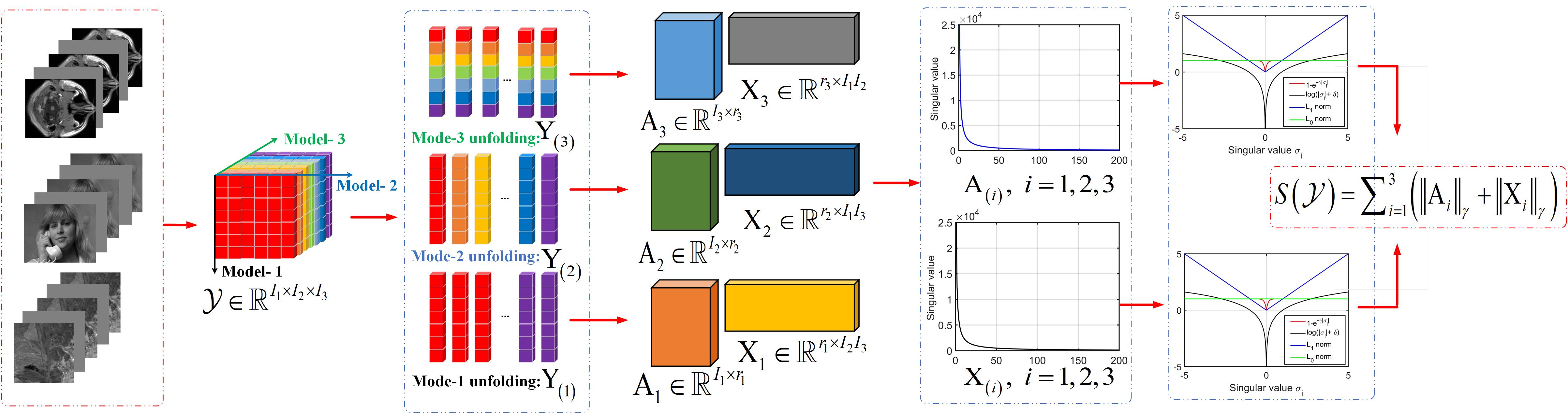
Figure 2: Flowchart of the proposed low-rank tensor approximation: nonconvex tensor $L_{\gamma}$ norm.

Then, to alleviate bias phenomenons of the TNN minimization in tensor completion tasks, Jiang et al. [22] represent the low-rank prior of underlying tensor by using the PSTNN. The PSTNN regularized tensor completion model is formulated as follows:

$$\arg\min_{\mathcal{Y}}\frac{1}{I_{3}}\sum_{i=1}^{I_{3}}\left\|\bar{\mathbf{Y}}^{(i)}\right\|_{p=M},s.t.~{}\mathcal{P}_{\Omega}(\mathcal{Y})=\mathcal{F},$$ (7)

where

$$\|\bar{\mathbf{Y}}^{(i)}\|_{p=M}:=\sum_{j=M+1}^{\min(I_{1},I_{2})}\sigma_{j}(\bar{\mathbf{Y}}^{(i)}),$$

and $\sigma_{j}(\bar{\mathbf{Y}}^{(i)})$ denotes the $j$-th largest singular value of $\bar{\mathbf{Y}}^{(i)}$.

To reduce the burden of calculating SVDs in TNN and PSTNN, Liu et al. [18] unfold the $N$-order tensor into multiple modal matrices along the direction of each mode, and then use the sum of the nuclear norms of these modal matrices, i.e., SNN, to describe the low-rank structure of the underlying tensor. With that definition, the completion model is formulated as follows:

$$\arg\min_{\mathcal{Y}}\sum_{n=1}^{N}\alpha_{i}\left\|\mathbf{Y}_{(n)}\right\|_{*},s.t.,\mathcal{P}_{\Omega}(\mathcal{Y})=\mathcal{F}.$$ (8)

Furthermore, Xu et al. [31] propose a Tmac model by using parallel matrix factorization, which obtain promising results with less computational complexity than TNN and PSTNN,

$$\arg\min_{\mathcal{Y},\mathbf{X},\mathbf{A}}\sum_{n=1}^{N}\frac{\alpha_{n}}{2}\left\|\mathbf{Y}_{(n)}-\mathbf{A}_{n}\mathbf{X}_{n}\right\|_{F}^{2},$$ (9)

$$\text{ s.t. }\quad\mathcal{P}_{\Omega}(\mathcal{Y})=\mathcal{F},$$

where $\alpha_{n}$ are weights and satisfy $\sum_{n=1}^{N}\alpha_{n}=1$.

Although the above-mentioned low-rank tensor completion methods report success on dealing with a large variety of tasks, there are several open issues which have yet to be addressed. Firstly, the above approaches either explore the low-rank prior lying in only one mode of the underlying tensor or directly represent the low-rank prior of original tensor by using low-rank decomposition. They do not further explore the prior of the factors (e.g., $\mathbf{A}_{n},\mathbf{X}_{n}$ in (9)) obtained by low-rank decomposition. Secondly, TNN based methods [33, 22, 10] need to compute lots of SVDs, which is time-consuming or even not applicable for large-scale problems [31]. Thirdly, these methods adopt single surrogate of tensor rank function, which would cause suboptimal solution of the low-rank tensor completion problems [34] and can not fully explore the low-rank priors in all modes, especially when the tensor data is heavily contaminated or the sampling rate is very low. One can see an example in Fig. 1, in which the video ”suzie” with 95% missing entries, it can be seen that our model restores most of the structural information of the video, while the videos restored by the methods adopt single surrogate contain only the outline of the images.

IV Double nonconvex $L_{\gamma}$ norm based low-rank approximation for tensor completion

In the following, a novel double nonconvex $L_{\gamma}$ norm based low-rank approximation of tensor multi-modes (LRATM) is introduced firstly. Then, the optimization of the proposed LRATM model is deduced in detail.

IV-A LRATM Model

For a tensor $\mathcal{Y}\in\mathbb{R}^{I_{1}\times I_{2}\times\cdots\times I_{N}}$, to enhance the flexibility for handling different correlations along different modes in the underlying tensor, while to effectively explore the underlying joint-manifold drawn from the mode factorization factors, we first formulate a nonconvex novel tensor $L_{\gamma}$ norm,

$$\left\|\mathcal{Y}\right\|_{\gamma}=\sum_{n=1}^{N}(\tau_{n}\left\|\mathbf{X}_{n}\right\|_{\gamma}+\lambda_{n}\left\|\mathbf{A}_{n}\right\|_{\gamma}),$$ (10)

where $\mathbf{Y}_{(n)}=\mathbf{A}_{n}\mathbf{X}_{n}$, and

$$\left\|\mathbf{X}\right\|_{\gamma}:=\sum_{t=1}^{\min\{p,q\}}\left(1-e^{-\sigma_{t}(\mathbf{X})/\gamma}\right)$$

is a nonconvex approximation of $rank(\mathbf{X})$, and $\sigma_{t}(\mathbf{X})$ is the $t$-th biggest singular value of $\mathbf{X}\in\mathbb{R}^{p\times q}$. $\tau_{n}$ and $\lambda_{n}$ are non-negative constants that balance the two terms.

Then, our tensor $L_{\gamma}$ norm based low-rank approximation model for low-rank tensor completion, i.e., the proposed LRATM model is written as

$$\arg\min{\left\|\mathcal{Y}\right\|_{\gamma}}= \arg\min_{\mathcal{Y},\mathbf{X},\mathbf{A}}\sum_{n=1}^{N}(\tau_{n}\left\|\mathbf{X}_{n}\right\|_{\gamma}+\lambda_{n}\left\|\mathbf{A}_{n}\right\|_{\gamma}),$$ (11)

$$s.t.,~{}\mathbf{Y}_{(n)}=\mathbf{A}_{n}\mathbf{X}_{n},\mathcal{P}_{\Omega}(\mathcal{Y})=\mathcal{F}.$$

To better understand the proposed LRATM model, we plot the flowchart of the proposed low-rank tensor approximation in Fig. 2. It can be seen that the video, MRI and HSI in the first column essentially can be viewed as 3-order tensors in the second column. When we unfold the 3-order tensor in three directions, the low-rank structure of all the $N$ modes can be explored by using parallel matrix decomposition, i.e., $\mathbf{Y}_{(n)}=\mathbf{A}_{n}\mathbf{X}_{n},n=1,2,\cdots,N$, which is computationally much cheaper than SVD. The decomposed factors have practical physical meaning, $\mathbf{A}_{n}$ represents a library (each column contains a signature of the $n$-th mode direction), and $\mathbf{X}_{n}$ is called an encoding. For example, in the unmixing problem for HSI [35], each column of $\mathbf{A}_{3}$ contains a spectral signature, and each row of $\mathbf{X}_{3}$ contains the fractional abundances of a given endmembers. This interpretation is also valid for the mode-3 unfolding of video and MRI. The above parallel matrix decomposition can effectively explore the low-rank structure of underlying tensor, but the prior information contained in the factor matrices ($\mathbf{A}_{n},\mathbf{X}_{n}$) is not explored at all. Therefore, to further enhance the potential capacity of tensor completion models, it is necessary to design new and reasonable formulas to explore the priors in the factor matrices. Here, we propose the novel nonconvex double $L_{\gamma}$ norm to formulate the underlying joint-manifold drawn from the mode factorization factors $\mathbf{A}_{n}$ and $\mathbf{X}_{n}$. The superiority of $L_{\gamma}$ norm over nuclear norm and other nonconvex penalties is shown in the fifth column of Fig. 2. It is obvious that the red curve of $L_{\gamma}$ norm is closer to the green curve of $L_{0}$ norm (rank function) than other nonconvex penalties.

IV-B Optimization Procedure of LRATM

In this section, the proposed model is solved by using the block successive upper-bound minimization (BSUM) [36] method. The objective function of the proposed LRATM model(11) can be formulated as follows:

$$f(\mathbf{X},\mathbf{A},\mathcal{Y})=\sum_{n=1}^{N} \left(\frac{\alpha_{n}}{2}\left\|\mathbf{Y}_{(n)}-\mathbf{A}_{n}\mathbf{X}_{n}\right\|_{\text{F}}^{2}+\tau_{n}\left\|\mathbf{X}_{n}\right\|_{\gamma}\right.$$ (12)

$$\left.+\lambda_{n}\left\|\mathbf{A}_{n}\right\|_{\gamma}\right).$$

According to the proximal operator (3), the update can be written as:

$$p(\mathcal{S},\mathcal{S}^{k})=f\left(\mathcal{S},\mathcal{S}^{k}\right)+\frac{\rho}{2}\left\|\mathcal{S}-\mathcal{S}^{k}\right\|_{\text{F}}^{2},$$ (13)

where $\rho>0$ is a positive constant; $\mathcal{S}=(\mathbf{X},\mathbf{A},\mathcal{Y})$ and $\mathcal{S}^{k}=\left(\mathbf{X}^{k},\mathbf{A}^{k},\mathcal{Y}^{k}\right)$. Let

$$\left\{\begin{array}[]{l}g_{1}\left(\mathbf{X},\mathcal{S}_{1}^{k}\right)=f\left(\mathbf{X},\mathbf{A}^{k},\mathcal{Y}^{k}\right)+\frac{\rho}{2}\left\|\mathbf{X}-\mathbf{X}^{k}\right\|_{\text{F}}^{2},\\ g_{2}\left(\mathbf{A},\mathcal{S}_{2}^{k}\right)=f\left(\mathbf{X}^{k+1},\mathbf{A},\mathcal{Y}^{k}\right)+\frac{\rho}{2}\left\|\mathbf{A}-\mathbf{A}^{k}\right\|_{\text{F}}^{2,}\\ g_{3}\left(\mathcal{Y},\mathcal{S}_{3}^{k}\right)=f\left(\mathbf{X}^{k+1},\mathbf{A}^{k+1},\mathcal{Y}\right)+\frac{\rho}{2}\left\|\mathcal{Y}-\mathcal{Y}^{k}\right\|_{\text{F}}^{2},\end{array}\right.$$ (14)

where

$$\left\{\begin{array}[]{l}S_{1}^{k}=\left(\mathbf{X}^{k},\mathbf{A}^{k},\mathcal{Y}^{k}\right),\\ S_{2}^{k}=\left(\mathbf{X}^{k+1},\mathbf{A}^{k},\mathcal{Y}^{k}\right),\\ S_{3}^{k}=\left(\mathbf{X}^{k+1},\mathbf{A}^{k+1},\mathcal{Y}^{k}\right).\end{array}\right.$$ (15)

Then, problem (13) can be rewritten as follows:

$$\left\{\begin{array}[]{l}\displaystyle\mathbf{X}^{k+1}=\arg\min_{\mathbf{X}}g_{1}\left(\mathbf{X},\mathcal{S}_{1}^{k}\right),\\ \displaystyle\mathbf{A}^{k+1}=\arg\min_{\mathbf{A}}g_{2}\left(\mathbf{A},\mathcal{S}_{2}^{k}\right),\\ \displaystyle\mathcal{Y}^{k+1}=\arg\min_{\mathcal{P}_{\Omega}(\mathcal{Y})=\mathcal{F}}g_{3}\left(\mathcal{Y},\mathcal{S}_{3}^{k}\right).\end{array}\right.$$ (16)

IV-B1 Update $\mathbf{X}_{n}$

With fixing other variables, the optimization subproblem with respect to $\mathbf{X}_{n},n=1,2,\cdots,N$, in (16) can be written as follows:

$$\arg\min_{\{\mathbf{X}_{n}\}_{n=1}^{N}}\sum_{n=1}^{N} \left(\frac{\alpha_{n}}{2}\left\|\mathbf{Y}_{(n)}-\mathbf{A}_{n}\mathbf{X}_{n}\right\|_{\text{F}}^{2}+\tau_{n}\left\|\mathbf{X}_{n}\right\|_{\gamma}\right.$$ (17)

$$\left.+\frac{\rho_{n}}{2}\left\|\mathbf{X}_{n}-\mathbf{X}_{n}^{k}\right\|_{\text{F}}^{2}\right).$$

To efficiently solve the above optimization, we first introduce auxiliary variables $\mathbf{X}_{n}=\mathbf{Z}_{n},n=1,2,\cdots,N$. Then, by the augmented Lagrangian multiplier (ALM) method, the optimization subproblem (17) can be rewritten as:

$$\arg\min_{\{\mathbf{X}_{n},\{\mathbf{Z}_{n}\}_{n=1}^{N}}\sum_{n=1}^{N}\left(\frac{\alpha_{n}}{2}\left\|\mathbf{Y}_{(n)}-\mathbf{A}_{n}\mathbf{X}_{n}\right\|_{\text{F}}^{2}+\tau_{n}\left\|\mathbf{Z}_{n}\right\|_{\gamma}\right.$$ (18)

$$\left.+\frac{\rho_{n}}{2}\left\|\mathbf{X}_{n}-\mathbf{X}_{n}^{k}\right\|_{\text{F}}^{2}+\left\langle\Gamma_{n}^{\mathbf{X}},\mathbf{X}_{n}-\mathbf{Z}_{n}\right\rangle+\frac{\rho_{n}}{2}\left\|\mathbf{X}_{n}-\mathbf{Z}_{n}\right\|_{\text{F}}^{2}\right).$$

where $\Gamma_{n}^{\mathbf{X}}$ are Lagrangian multipliers.

With other variables fixed, the minimization subproblem for $\mathbf{Z}_{n}$ can be deduced from (18) as follows:

$$\mathbf{Z}_{n}^{k+1}=\arg\min_{\mathbf{Z}_{n}}\left\|\mathbf{Z}_{n}\right\|_{\gamma}+\frac{\hat{\rho}_{n}}{2}\left\|\mathbf{Z}_{n}-\mathbf{P}_{n}^{k}\right\|_{\text{F}}^{2},$$ (19)

where $\hat{\rho}_{n}=\rho_{n}/\tau_{n}$, $\mathbf{P}_{n}^{k}=\mathbf{X}_{n}^{k}+\Gamma_{n}^{\mathbf{X}}/\rho_{n}$. Let $\sigma_{1}^{k}\geq\sigma_{2}^{k}\geq\cdots\geq\sigma_{t_{n}}^{k}$ represent the singular values of $\mathbf{Z}_{n}^{k}\in\mathbb{R}^{r_{n}\times s_{n}}$ with $t_{n}=\min\left\{r_{n},s_{n}\right\}$ and $\nabla\phi\left(\sigma_{n}^{k}\right)$ denote the gradient of $\phi(x)=1-e^{-x/\gamma}$ at $\sigma_{n}^{k}.$ Let

$$f(\mathbf{Z}_{n})=\frac{1}{2}\left\|\mathbf{Z}_{n}-\mathbf{P}_{n}^{k}\right\|_{\text{F}}^{2}.$$

It is easy to prove that the gradient of $f(\mathbf{Z}_{n})$ is Lipschitz continuous by setting the Lipschitz constant being $1.$ As stated in [30], considering the nonascending order of singular values and according to the antimonotone property of gradient of our nonconvex function, we have

$$0\leq\nabla\phi\left(\sigma_{1}^{k}\right)\leq\nabla\phi\left(\sigma_{2}^{k}\right)\leq\cdots\leq\nabla\phi\left(\sigma_{t_{n}}^{k}\right),$$ (20)

$$\phi\left(\sigma_{i}(\mathbf{Z}_{n})\right)\leq\phi\left(\sigma_{i}^{k}\right)+\nabla\phi\left(\sigma_{i}^{k}\right)\left(\sigma_{i}(\mathbf{Z}_{n})-\sigma_{i}^{k}\right),$$

where $i=1,2,\cdots,t_{n}$. Following (20), the subproblem with respect to $\mathbf{Z}_{n}$ (19) can be written as following relaxation:

$$\begin{split}&\arg\min_{\mathbf{Z}_{n}}\frac{1}{\hat{\rho}_{n}}\sum_{n=1}^{t_{n}}\phi\left(\sigma_{n}^{k}\right)+\nabla\phi\left(\sigma_{n}^{k}\right)\left(\sigma_{n}(\mathbf{Z}_{n})-\sigma_{n}^{k}\right)+f(\mathbf{Z}_{n})\\ &=\arg\min_{\mathbf{Z}_{n}}\frac{1}{\hat{\rho}_{n}}\sum_{n=1}^{t_{n}}\nabla\phi\left(\sigma_{n}^{k}\right)\sigma_{n}(\mathbf{Z}_{n})+\frac{1}{2}\left\|\mathbf{Z}_{n}-\mathbf{P}_{n}^{k}\right\|_{\text{F}}^{2}.\end{split}$$ (21)

Then, based on [37, 30], the solution of (21) can be efficiently obtained by generalized weight singular value thresholding (WSVT) [38] , as shown in Lemma 1.

Lemma 1: For any $1/\hat{\rho}_{n}>0$, the given data $\mathbf{P}_{n}^{k}=\mathbf{X}_{n}^{k}+\Gamma_{n}^{\mathbf{X}}/\rho_{n}$, and $0\leq\nabla\phi\left(\sigma_{1}^{k}\right)\leq\nabla\phi\left(\sigma_{2}^{k}\right)\leq\cdots\leq\nabla\phi\left(\sigma_{t_{n}}^{k}\right)$, a globally optimal solution $\mathbf{Z}_{n}^{*}$ to (21) is given as follows:

$$\quad\mathbf{Z}_{n}^{k+1}=\operatorname{WSVT}\left(\mathbf{P}_{n}^{k},\frac{\nabla\phi}{\hat{\rho}_{n}}\right)=\mathbf{U}\mathbf{S}_{\frac{\nabla\phi}{\hat{\rho}_{n}}}(\mathbf{\Sigma})\mathbf{V}^{T},$$ (22)

where $\mathbf{P}_{n}^{k}=\mathbf{U}\mathbf{\Sigma}\mathbf{V}^{T}$ is the SVD of $\mathbf{P}_{n}^{k}$;

$$\mathbf{S}_{\frac{\nabla\phi}{\hat{\rho}_{n}}}(\mathbf{\Sigma})=\operatorname{Diag}\left\{\max\left(\mathbf{\Sigma}_{ii}-\frac{\nabla\phi\left(\mathbf{\sigma}_{i}^{k}\right)}{\hat{\rho}_{n}},0\right)\right\},$$

and $i=1,2,\cdots,t_{n}$.

With other variables fixed, the minimization subproblem for $\mathbf{X}_{n}$, $n=1,2,\cdots,N$, can be deduced from (18) as follows:

$$\mathbf{X}_{n}^{k+1} =\arg\min_{\mathbf{X}_{n}}\frac{\alpha_{n}}{2}\left\|\mathbf{Y}_{(n)}-\mathbf{A}_{n}^{k}\mathbf{X}_{n}\right\|_{\text{F}}^{2}$$ (23)

$$+\frac{\rho_{n}}{2}\left\|\mathbf{X}_{n}-\frac{\mathbf{Z}_{n}^{k+1}-\Gamma_{n}^{k}/\mu_{n}+\mathbf{X}_{n}^{k}}{2}\right\|_{\text{F}}^{2}.$$

They are convex and have the following closed-form solutions

$$\mathbf{X}_{n}^{k+1}= \frac{1}{2}(\alpha_{n}\mathbf{A}_{n}^{T}\mathbf{A}_{n}+2\rho_{n}\mathbf{I}_{n})^{-1}\left[2\alpha_{n}\mathbf{A}_{n}^{T}\mathbf{Y}_{(n)}\right.$$ (24)

$$\left.+\mu_{n}\left(\mathbf{Z}_{n}^{k+1}-\Gamma_{n}^{k}/\mu_{n}+\mathbf{X}_{n}^{k}\right)\right].$$

The Lagrangian multipliers $\Gamma_{n}^{\mathbf{X}}$ can be updated by the following equation

$$\Gamma_{n}^{\mathbf{X}}=\Gamma_{n}^{\mathbf{X}}+\mathbf{X}_{n}-\mathbf{Z}_{n}.$$ (25)

IV-B2 Update $\mathbf{A}_{n}$

With fixing other variables, the optimization subproblem with respect to $\mathbf{A}_{n}$, $n=1,2,\cdots,N$, in (16) can be written as follows:

$$\arg\min_{\{\mathbf{A}_{n}\}_{n=1}^{N}}\sum_{n=1}^{N} \left(\frac{\alpha_{n}}{2}\left\|\mathbf{Y}_{(n)}-\mathbf{A}_{n}\mathbf{X}_{n}\right\|_{\text{F}}^{2}+\lambda_{n}\left\|\mathbf{A}_{n}\right\|_{\gamma}\right.$$ (26)

$$\left.+\frac{\rho_{n}}{2}\left\|\mathbf{A}_{n}-\mathbf{A}_{n}^{k}\right\|_{\text{F}}^{2}\right).$$

To efficiently solve the above optimization, we first introduce auxiliary variables $\mathbf{A}_{n}=\mathbf{J}_{n},n=1,2,\cdots,N$. Then, by the ALM method, the problem (26) can also be reformulated as

$$\arg\min_{\{\mathbf{A}_{n},\mathbf{J}_{n}\}_{n=1}^{N}}\sum_{n=1}^{N}\left(\frac{\alpha_{n}}{2}\left\|\mathbf{Y}_{(n)}-\mathbf{A}_{n}\mathbf{X}_{n}\right\|_{\text{F}}^{2}+\lambda_{n}\left\|\mathbf{J}_{n}\right\|_{\gamma}\right.$$ (27)

$$\left.+\frac{\rho_{n}}{2}\left\|\mathbf{A}_{n}-\mathbf{A}_{n}^{k}\right\|_{\text{F}}^{2}+\left\langle\Gamma_{n}^{\mathbf{A}},\mathbf{A}_{n}-\mathbf{J}_{n}\right\rangle+\frac{\rho_{n}}{2}\left\|\mathbf{A}_{n}-\mathbf{J}_{n}\right\|_{\text{F}}^{2}\right),$$

where $\Gamma_{n}^{\mathbf{A}}$ are the Lagrangian multipliers.

With other variables fixed, the minimization subproblem for $\mathbf{J}_{n}$ can be deduced from (27) as follows:

$$\mathbf{J}_{n}^{k+1}=\arg\min_{\mathbf{J}_{n}}\lambda_{n}\left\|\mathbf{J}_{n}\right\|_{\gamma}+\frac{\rho_{n}}{2}\left\|\mathbf{J}_{n}-\mathbf{Q}_{n}^{k}\right\|_{\text{F}}^{2}.$$ (28)

where $\tilde{\rho}_{n}=\rho_{n}/\lambda_{n}$; $\mathbf{Q}_{n}^{k}=\mathbf{A}_{n}^{k}+\Gamma_{n}^{\mathbf{A}}/\rho_{n}$. Its solution can also be obtained by Lemma 1 as follows:

$$\quad\mathbf{J}_{n}^{k+1}=\operatorname{WSVT}\left(\mathbf{Q}_{n}^{k},\frac{\nabla\phi}{\tilde{\rho}_{n}}\right).$$ (29)

With other variables fixed, the minimization subproblem for $\mathbf{A}_{n}$, $n=1,2,\cdots,N$, can be deduced from (27) as follows:

$$\mathbf{A}_{n}^{k+1}= \arg\min_{\mathbf{A}_{n}}\frac{\alpha_{n}}{2}\left\|\mathbf{Y}_{(n)}-\mathbf{A}_{n}\mathbf{X}_{n}\right\|_{\text{F}}^{2}$$ (30)

$$+\rho_{n}\left\|\mathbf{A}_{n}-\frac{\mathbf{J}_{n}^{k+1}-\Gamma_{n}^{\mathbf{A}}/\rho_{n}+\mathbf{A}_{n}^{k}}{2}\right\|_{\text{F}}^{2}.$$

They are also convex and have the following closed-form solutions

$$\mathbf{A}_{n}^{k+1}= \left(\mathbf{Y}_{(n)}^{k}\left(\mathbf{X}_{n}^{k+1}\right)^{T}+\rho_{n}(\mathbf{J}_{n}^{k+1}-\Gamma_{n}^{\mathbf{A}}/\rho_{n}+\mathbf{A}_{n}^{k})\right)$$ (31)

$$\left(\mathbf{X}_{n}^{k+1}\left(\mathbf{X}_{n}^{k+1}\right)^{T}+2\rho_{n}\mathbf{I}_{n}\right)^{\dagger}.$$

Finally, the Lagrangian multipliers $\Gamma_{n}^{\mathbf{A}}$ can be updated by the following equation

$$\Gamma_{n}^{\mathbf{A}}=\Gamma_{n}^{\mathbf{A}}+\mathbf{A}_{n}-\mathbf{J}_{n}.$$ (32)

IV-B3 Update $\mathcal{Y}$

With other variables fixed, the minimization subproblem with respect to $\mathcal{Y}$ in (16) can be written as

$$\arg\min_{\{\mathbf{Y}_{(n)}\}_{n=1}^{N}}\sum_{n=1}^{N}\frac{\alpha_{n}}{2}\left\|\mathbf{Y}_{(n)}-\mathbf{A}_{n}\mathbf{X}_{n}\right\|_{\text{F}}^{2}+\frac{\rho}{2}\left\|\mathcal{Y}-\mathcal{Y}^{k}\right\|_{\text{F}}^{2}$$ (33)

$$s.t.,\mathcal{P}_{\Omega}(\mathcal{Y})=\mathcal{F}.$$

Then, the update of $\mathcal{Y}^{k+1}$ can be written explicitly as

$$\begin{array}[]{l}\displaystyle\mathcal{Y}^{k+1}=\mathcal{P}_{{\Omega}^{c}}\left(\sum_{n=1}^{N}\alpha_{n}\text{ fold }_{n}\left(\frac{\mathbf{A}_{n}^{k+1}\mathbf{X}_{n}^{k+1}+\rho_{n}\mathbf{Y}_{(n)}^{k}}{1+\rho_{n}}\right)\right)+\mathcal{F},\end{array}$$ (34)

where $\Omega^{C}$ is the complementary set of $\Omega$.

Algorithm 1 :Algorithm for the LRATM model.

1:The observed tensor $\mathcal{F}$; The set of index of observed entries $\Omega$; Stopping criterion $\varepsilon$, the given $n$-rank, $r=\left(r_{1},r_{2},r_{3}\right)$.

2:The completed tensor.

3:Initialize: $\mathbf{X}_{n}=\mathbf{Z}_{n}=0,\mathbf{A}_{n}=\mathbf{J}_{n}=0,\Gamma_{n}^{\mathbf{X}}=0,\Gamma_{n}^{\mathbf{A}}=0,n=1,2,\cdots,N$; $k=0$.

4:Repeat until convergence:

5:Update $\mathbf{X},\mathbf{Z},\mathbf{A},\mathbf{J},\mathcal{Y},\Gamma^{\mathbf{X}},\Gamma^{\mathbf{A}}$ via 1st step: Update $\mathbf{Z}_{n}$ via (22) 2nd step: Update $\mathbf{X}_{n}$ via (24) 3rd step: Update $\mathbf{A}_{n}$ via (31) 4th step: Update $\mathbf{J}_{n}$ via (29) 5th step: Update $\mathcal{Y}$ via (34) 6th step: Update the parameter via (25), (32)

6:Check the convergence condition.

IV-C Complexity and Convergence Analysis

The proposed algorithm for our LRATM model is summarized in Algorithm 1. Further, we discuss the complexity and convergence of the proposed algorithm.

IV-C1 Complexity analysis

The cost of computing $\mathbf{X}_{n}$ is $O\left(I_{n}r_{n}^{2}+I_{n}r_{n}s_{n}+r_{n}^{2}s_{n}\right)$, calculating $\mathbf{Z_{n}}$ has a complexity of $O\left(\Pi_{j\neq n}I_{j}\times r_{n}^{2}\right)$, the complexity of updating $\mathbf{J}_{n}$ is $O\left(I_{n}r_{n}^{2}\right)$, calculating $\mathbf{A}_{n}$ has a complexity of $O\left(I_{n}r_{n}^{2}+I_{n}r_{n}s_{n}+r_{n}^{2}s_{n}\right)$, calculating $\mathcal{Y}$ has a complexity of $O\left(r_{1}I_{1}s_{1}+\cdots+r_{N}I_{N}s_{N}\right)$. Therefore, the total complexity of the proposed algorithm can be obtained by counting the complexity of the above variables, i.e.,

$$O\left(\sum_{n}(3I_{n}r_{n}^{2}+\Pi_{j\neq n}I_{j}\times r_{n}^{2}+3I_{n}r_{n}S_{n}+2r_{n}^{2}s_{n})\right).$$ (35)

IV-C2 Convergence analysis

In this section, we theoretically analyze the convergence of the proposed algorithm by using the BSUM method [36].

Lemma 2 [36]: Let us assume that the feasible set $\mathcal{X}$ is the cartesian product of $n$ closed convex sets: $\mathcal{X}=\mathcal{X}_{1}\times\mathcal{X}_{2}\times\cdots\times\mathcal{X}_{n}$. Given the problem

$$\min f(x),s.t.~{}x\in\mathcal{X},$$ (36)

assume $h\left(x,x^{k-1}\right)$ is an approximation of $f(x)$ at the $(k-1)$-th iteration, which satisfies the following conditions:

$$\begin{array}[]{l}1)\quad h_{i}\left(y_{i},y\right)=f(y),\forall y\in\mathcal{X},\forall i;\\ 2)\quad h_{i}\left(x_{i},y\right)\geq f\left(y_{1},\ldots,y_{i-1},x_{i},y_{i+1},\ldots,y_{n}\right),\\ \quad\quad\forall x_{i}\in\mathcal{X}_{i},\forall y\in\mathcal{X},\forall i;\\ 3)\quad\left.h_{i}^{\prime}\left(x_{i},y;d_{i}\right)\right|_{x_{i}=y_{i}}=f^{\prime}(y;d),\forall d=\left(0,\cdots,d_{i}\cdots 0\right)\\ \quad\quad\text{ s.t. }y_{i}+d_{i}\in\mathcal{X}_{i},\forall i;\\ 4)\quad h_{i}\left(x_{i},y\right)\text{is continuous in}\left(x_{i},y\right),\forall i;\end{array}$$ (37)

where $h_{i}\left(x_{i},y\right)$ is the sub-problem with respect to the $i$-th block and $f^{\prime}(y;d)$ is the direction derivative of fat the point $y$ in direction $d$. Suppose $h_{i}\left(x_{i},y\right)$ is quasi-convex in $x_{i}$ for $i=1,2,\cdots,n$. Furthermore, assume that each sub-problem $\arg\min h_{i}\left(x_{i},x^{k-1}\right),s.t.~{}x\in\mathcal{X}_{i}$ has a unique solution for any point $x^{k-1}\in\mathcal{X}.$ Then, the iterates generated by the BSUM algorithm converge to the set of coordinatewise minimum of $f$.

Theorem 1. The iterates generated by (13) converge to the set of coordinatewise minimizers.

Proof. It is easy to verify that $g\left(\mathcal{S},\mathcal{S}^{k}\right)$ is an approximation and a global upper bound of $f(\mathcal{S})$ at the $k$-th iteration, which satisfies the following conditions:

$$\begin{array}[]{l}1)\quad g_{i}\left(\mathcal{S}_{i},\mathcal{S}\right)=f(\mathcal{S}),\forall\mathcal{S},i=1,2,3;\\ 2)\quad g_{i}\left(\bar{\mathcal{S}}_{i},\mathcal{S}\right)\geq f\left(\mathcal{S}_{1},\cdots,\bar{\mathcal{S}_{i}},\cdots,\mathcal{S}_{3}\right),\\ \quad\quad\forall\bar{\mathcal{S}}_{i},\forall\mathcal{S},i=1,2,3;\\ 3)\quad\left.g_{i}^{\prime}\left(\bar{\mathcal{S}}_{i},\mathcal{S};\mathbf{M}_{i}\right)\right|_{\bar{\mathcal{S}}_{i}=\mathcal{S}_{i}}=f^{\prime}\left(\mathcal{S};\mathbf{M}^{i}\right),\\ \quad\quad\forall\mathbf{M}^{i}=\left(0,\ldots,\mathbf{M}_{i},\ldots,0\right);\\ 4)\quad g_{i}\left(\bar{\mathcal{S}}_{i},\mathcal{S}\right)\text{is continuous in}\left(\bar{\mathcal{S}}_{i},\mathcal{S}\right),i=1,2,3;\end{array}$$ (38)

where $\mathcal{S}=(\mathbf{X},\mathbf{A},\mathcal{Y}),$ and $\mathcal{S}_{i}$ equal $\mathbf{X},\mathbf{A},\mathcal{Y}$ for $i=1,2,3,$ respectively. In addition, the subproblem $g_{i}(i=1,2,3)$ is quasi-convex with respect to $\mathbf{X},\mathbf{A}$ and $\mathcal{Y}$ respectively and each sub-problem of $g_{i}$ has a unique solution. Therefore, all assumptions in Lemma 1 are satisfied. According to the conclusion of Lemma 1, the Theorem 1 is valid, and the proposed algorithm is theoretically convergent.

V Numerical experiments

In this section, the proposed model is evaluated on three types of public tensor datasets, i.e., video datasets, MRI dataset and HSI dataset which have been frequently used to interpret the tensor completion performance of different models. To demonstrate its effectiveness, we compare the proposed model with TMac method [31], MF-TV method [32], single TNN based method [10] and PSTNN based method [22].

TABLE I: The averaged PSNR, SSIM, FSIM, ERGA and SAM of the completed results on video ”suzie” by Tmac, MF-TV, TNN, PSTNN and our model with different sampling rates. The best values are highlighted in bolder fonts.

			SR =0.05
PQI	nosiy	our model	MF-TV	TMac	PSTNN	TNN
PSNR	7.259	29.464	13.801	23.385	17.447	22.005
SSIM	0.009	0.807	0.094	0.622	0.192	0.563
FSIM	0.454	0.885	0.42	0.792	0.59	0.776
ERGA	1057.282	83.571	501.117	167.927	327.678	194.844
MSAM	77.324	3.622	24.095	6.927	13.775	7.797
			SR = 0.1
PQI	nosiy	our model	MF-TV	TMac	PSTNN	TNN
PSNR	7.493	32.056	22.356	26.189	26.647	26.032
SSIM	0.014	0.878	0.605	0.74	0.68	0.692
FSIM	0.426	0.924	0.758	0.838	0.843	0.846
ERGA	1029.096	62.314	196.059	124.369	117.104	124.923
MSAM	71.725	2.764	6.99	5.423	5.171	5.405
			SR = 0.2
PQI	nosiy	our model	MF-TV	TMac	PSTNN	TNN
PSNR	8.005	34.378	32.064	27.274	30.566	30.561
SSIM	0.02	0.918	0.872	0.782	0.829	0.831
FSIM	0.391	0.948	0.916	0.853	0.91	0.911
ERGA	970.285	47.877	66.692	109.627	75.472	75.598
MSAM	63.522	2.183	2.81	4.812	3.399	3.395

To accurately evaluate the performance of the test models, two types of standards are employed to quantitatively evaluate the quality of the completed tensors. The first one is the visual evaluation of the completed data, which is a qualitative evaluation standard. The second one is the five quantitative picture quality indices (PQIs), including the peak signal-to-noise ratio (PSNR) [39], structural similarity index (SSIM) [40], feature similarity (FSIM) [41], erreur relative globale adimensionnelle de synthèse (ERGAS) [42], the mean the spectral angle mapper (SAM) [43]. Larger PSNR, SSIM, FSIM and smaller ERGAS, SAM are, the better the completion performance of the corresponding model is. Since the experimental datasets are all third-order tensors, the PQIs for each frontal slice in the completed tensor are first calculated, and then the mean of these PQIs are finally used to evaluate the performance of the models. All experiments are performed on MATLAB 2019b, the CPU of the computer is Inter core i7@2.2GHz and the memory is 64GB. The code will be posted on the following URL: https://github.com/NavyZeng/LRATM.

V-A Video Data

(a) Original

(b) 95% Masked

(c) our model

(d) MF-TV

(e) Tmac

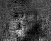
(f) PSTNN

(g) TNN

Figure 3: One slice of the recovered video for “suzie” by our model, MF-TV, Tmac, PSTNN and TNN. The sampling rate is 5%.

(a) Original

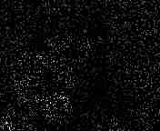
(b) 90% Masked

(c) our model

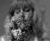
(d) MF-TV

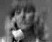
(e) Tmac

(f) PSTNN

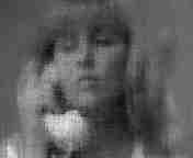
(g) TNN

Figure 4: One slice of the recovered video for “suzie” by our model, MF-TV, Tmac, PSTNN and TNN. The sampling rate is 10%.

(a) Original

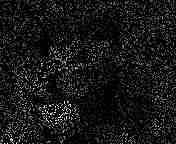
(b) 80% Masked

(c) our model

(d) MF-TV

(e) Tmac

(f) PSTNN

(g) TNN

Figure 5: One slice of the recovered video for “suzie” by our model, MF-TV, Tmac, PSTNN and TNN. The sampling rate is 20%.

In this subsection, we compare our model with MF-TV, Tmac, TNN and PSTNN on two video datasets: ”suzie” and “hall”, both of which are colored using YUV format, and two slices of them are shown in Fig. 3 and Fig. 6, respectively. Their sizes both are 144 $\times$ 176 $\times$ 150. We test all five methods on a series of sampling rates (SR): 5%, 10% and 20%, and all the test models are evaluated in terms of quantitative comparison and visual evaluation. In addition, the $n$-rank is approximated by using the number of the largest 0.5% singular values.

For quantitative comparison, Table I and Table II report the PQIs of the results completed by different methods. The best result for each PQI are marked in bold. From Table I and Table II, it can be found that our model obtains the highest indices among the five tested models in all SR cases; Tmac obtains the second best PQIs, when the SR is set to 5% or 10%; While MF-TV obtains the second best PQIs, when SR is set to 20%. The margins between the results by our model and the second best results are more than 5dB considering the PSNR.

For visual evaluation, we illustrate one frontal slice of the completed results with different sampling rates in Fig. 3, Fig. 4, Fig. 5, Fig. 6 and Fig. 7. It is clear from the figures that the results of our model are closest to the ground truth than other tested models, especially at low sampling rates. Specifically, as shown in Fig. 7, Fig. 3 and Fig. 4, when the sampling rates are 0.05 and 0.1, the advantages of our model are most obvious. Our model restores most of the structural information of the videos, while the videos restored by the competitive models contain only the outline of the images. At a higher sampling rate, as shown in Fig. 5 and Fig. 7, our model and competitive models both complete the main structural information of the images, but our model recovers more texture and detail information.

TABLE II: The averaged PSNR, SSIM, FSIM, ERGA and SAM of the recovered results on video ”hall” by Tmac, MF-TV, TNN, PSTNN and our model with different sampling rates. The best values are highlighted in bolder fonts.

			SR =0.05
PQI	nosiy	our model	MF-TV	TMac	PSTNN	TNN
PSNR	4.82	28.347	13.539	22.101	16.075	20.78
SSIM	0.007	0.894	0.412	0.675	0.36	0.636
FSIM	0.387	0.920	0.612	0.789	0.672	0.792
ERGA	1225.779	83.146	452.351	168.866	335.52	195.315
MSAM	77.299	2.360	12.865	3.818	8.64	4.299
			SR = 0.1
PQI	nosiy	our model	MF-TV	TMac	PSTNN	TNN
PSNR	5.055	31.804	24.855	26.936	29.014	28.433
SSIM	0.013	0.935	0.829	0.854	0.892	0.905
FSIM	0.393	0.950	0.873	0.888	0.934	0.936
ERGA	1193.075	56.998	131.422	97.185	77.395	82.259
MSAM	71.7	1.904	3.669	2.404	2.417	2.46
			SR = 0.2
PQI	nosiy	our model	MF-TV	TMac	PSTNN	TNN
PSNR	5.567	33.941	33.006	27.648	33.629	33.691
SSIM	0.025	0.952	0.94	0.869	0.961	0.962
FSIM	0.403	0.964	0.954	0.897	0.973	0.974
ERGA	1124.737	44.581	50.971	89.271	46.123	45.851
MSAM	63.507	1.574	1.779	2.226	1.584	1.565

V-B Magnetic resonance imaging data

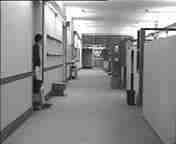
(a) Original

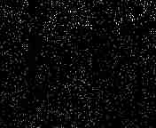
(b) 95% Masked

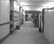
(c) our model

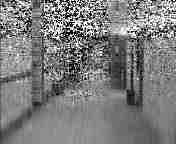
(d) MF-TV

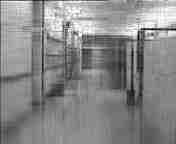
(e) Tmac

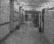
(f) PSTNN

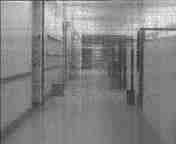
(g) TNN

Figure 6: One slice of the recovered video “hall” by our model, MF-TV, Tmac, PSTNN and TNN. The sampling rate is 5%.

(a) Original

(b) 90% Masked

(c) our model

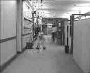
(d) MF-TV

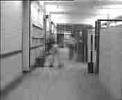
(e) Tmac

(f) PSTNN

(g) TNN

Figure 7: One slice of the recovered video “hall” by our model, MF-TV, Tmac, PSTNN and TNN. The sampling rate is 10%.

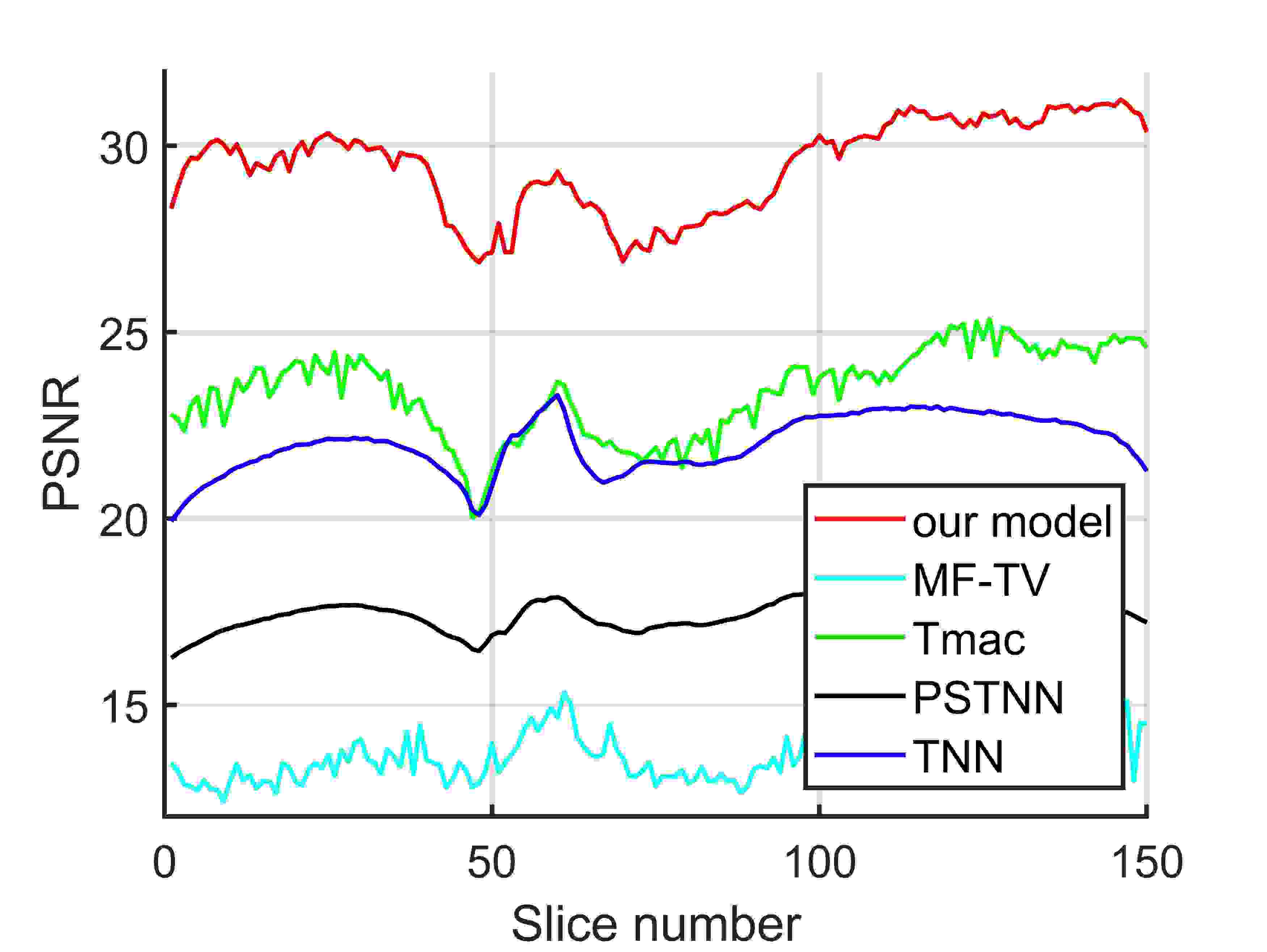
(a)

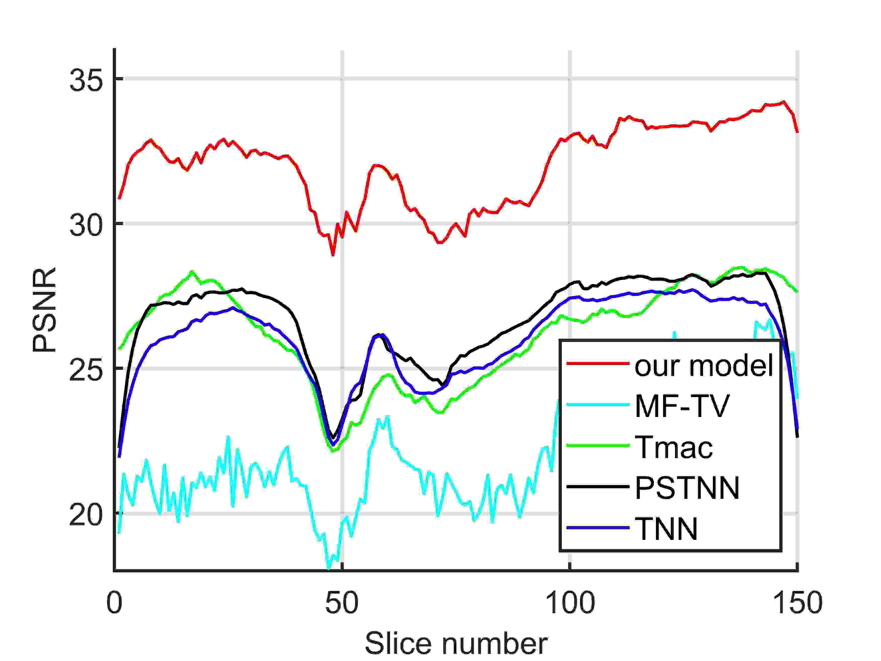
(b)

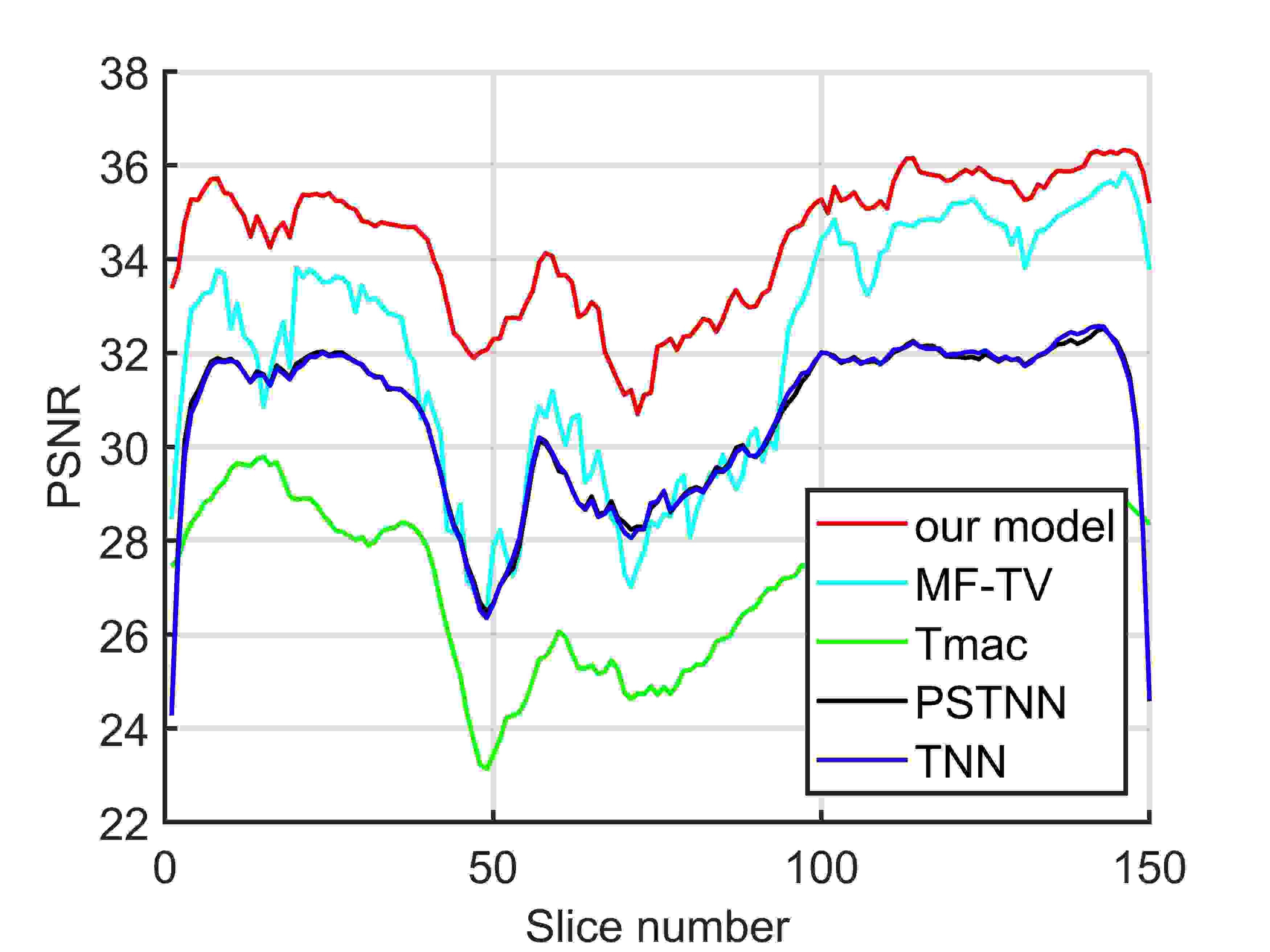
(c)

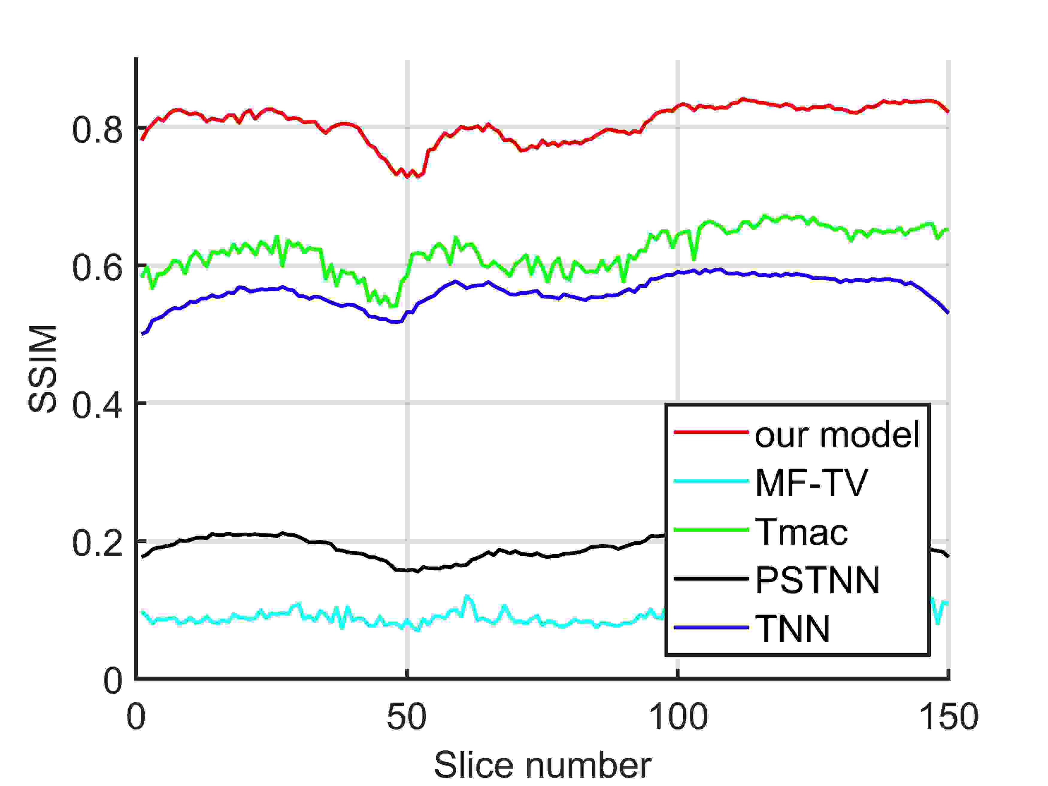
(d)

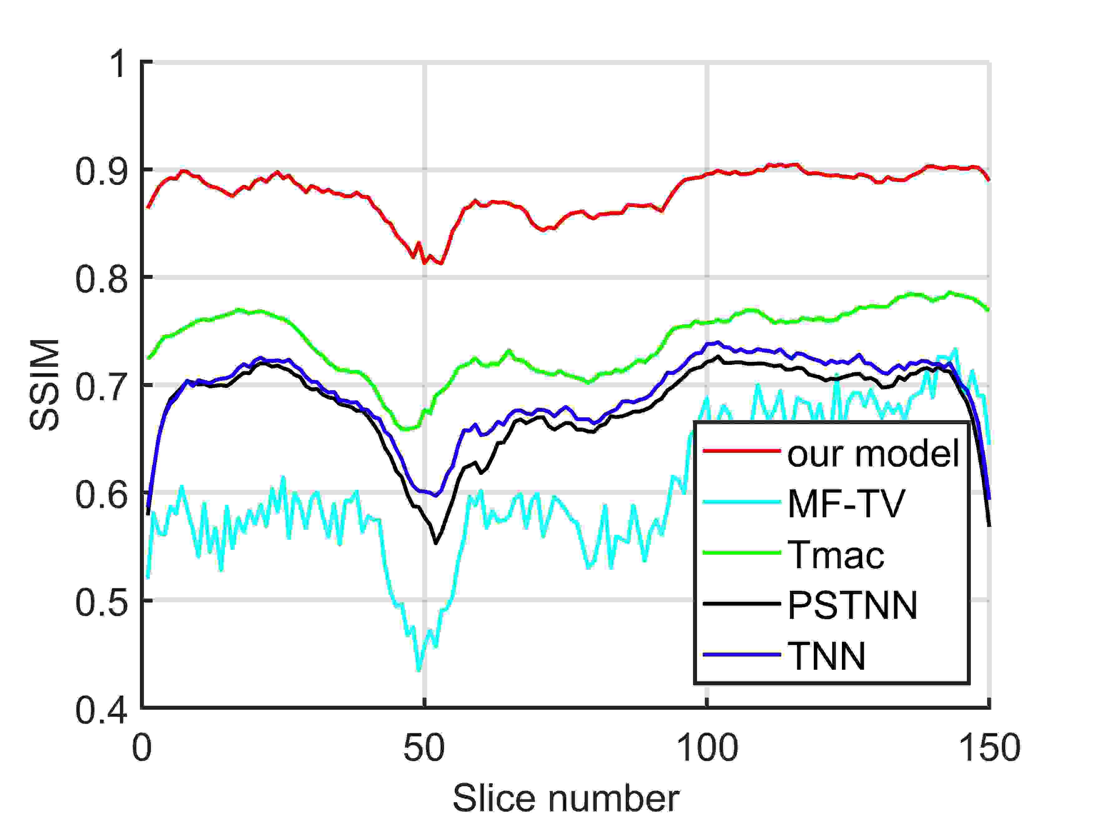
(e)

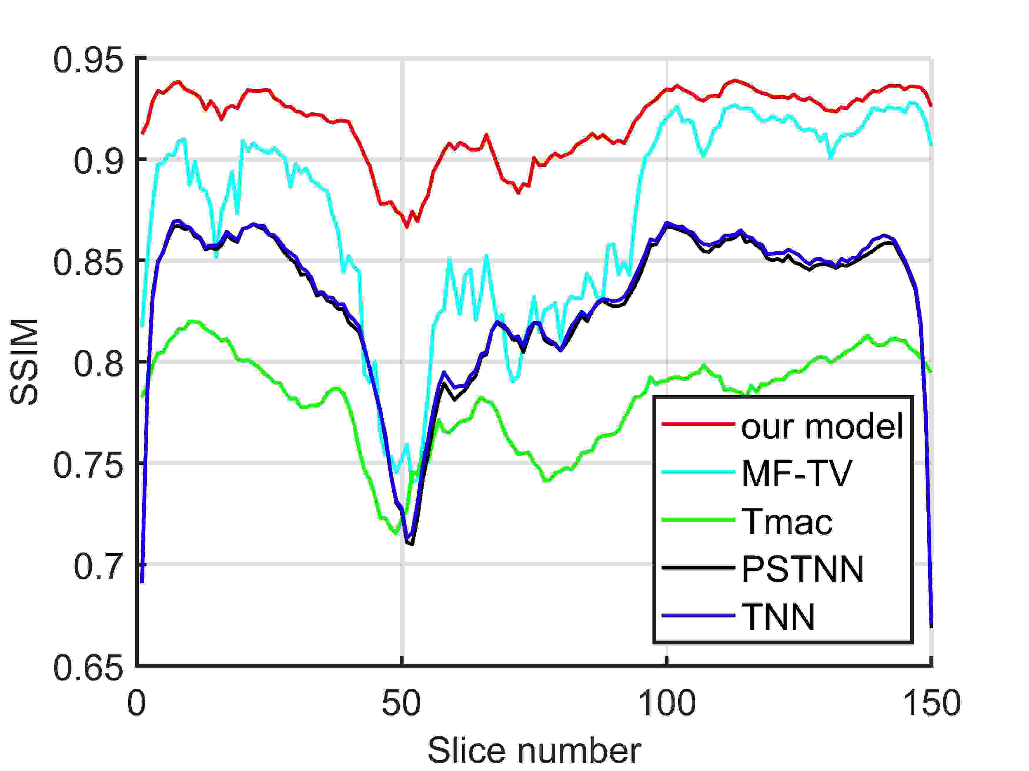
(f)

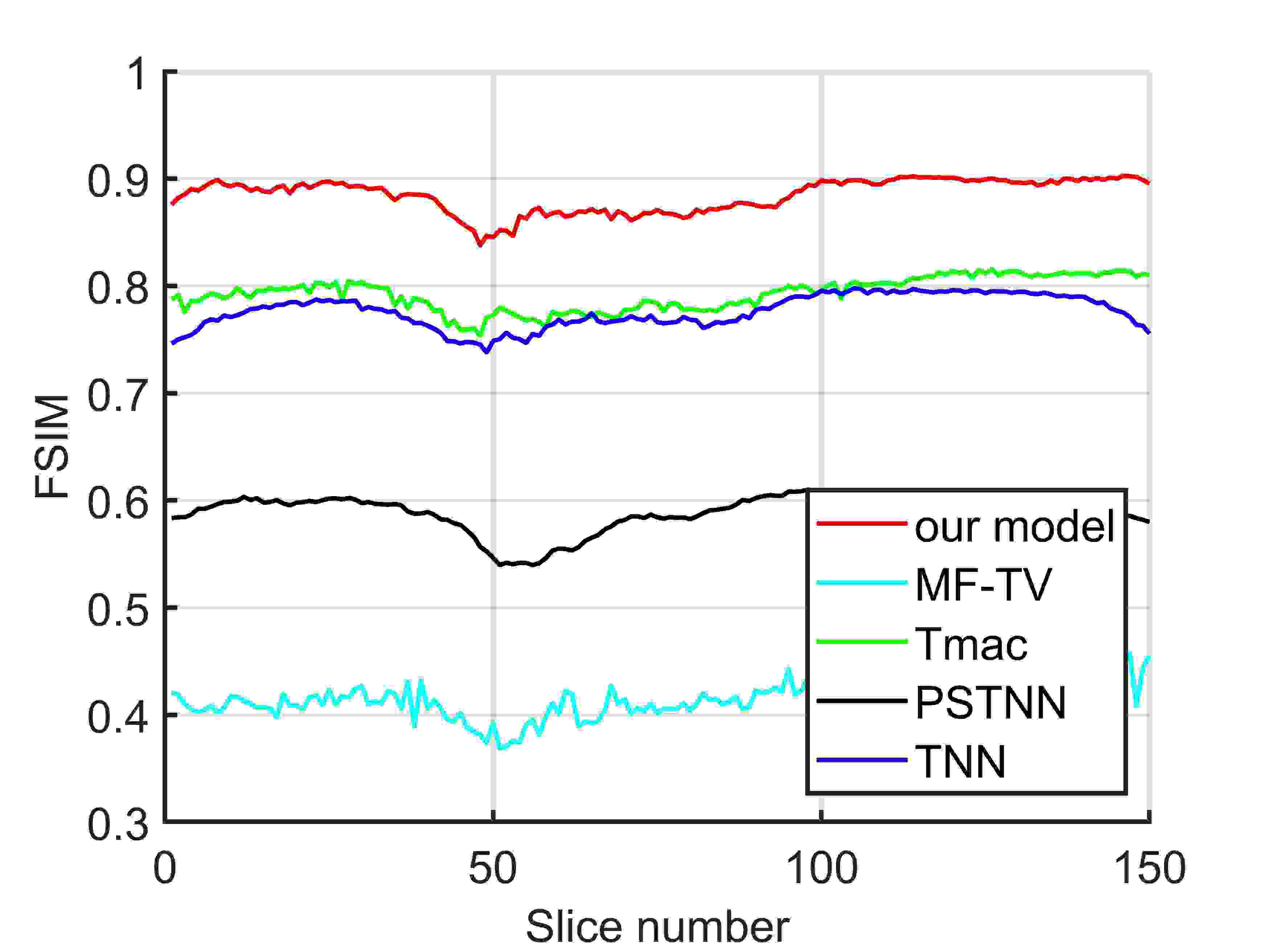
(g)

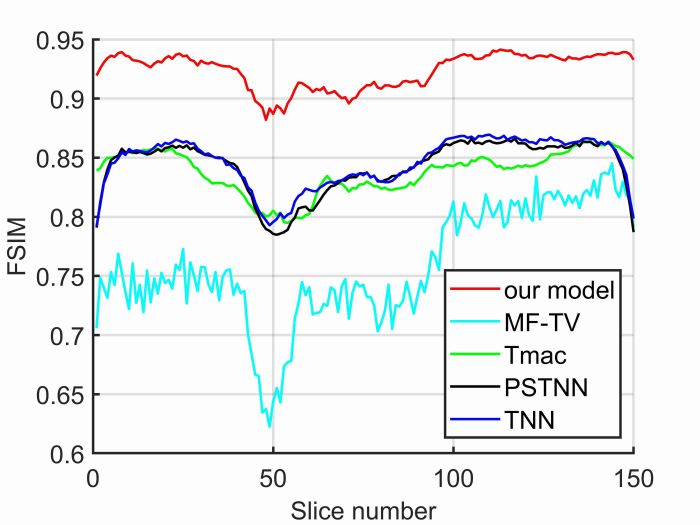
(h)

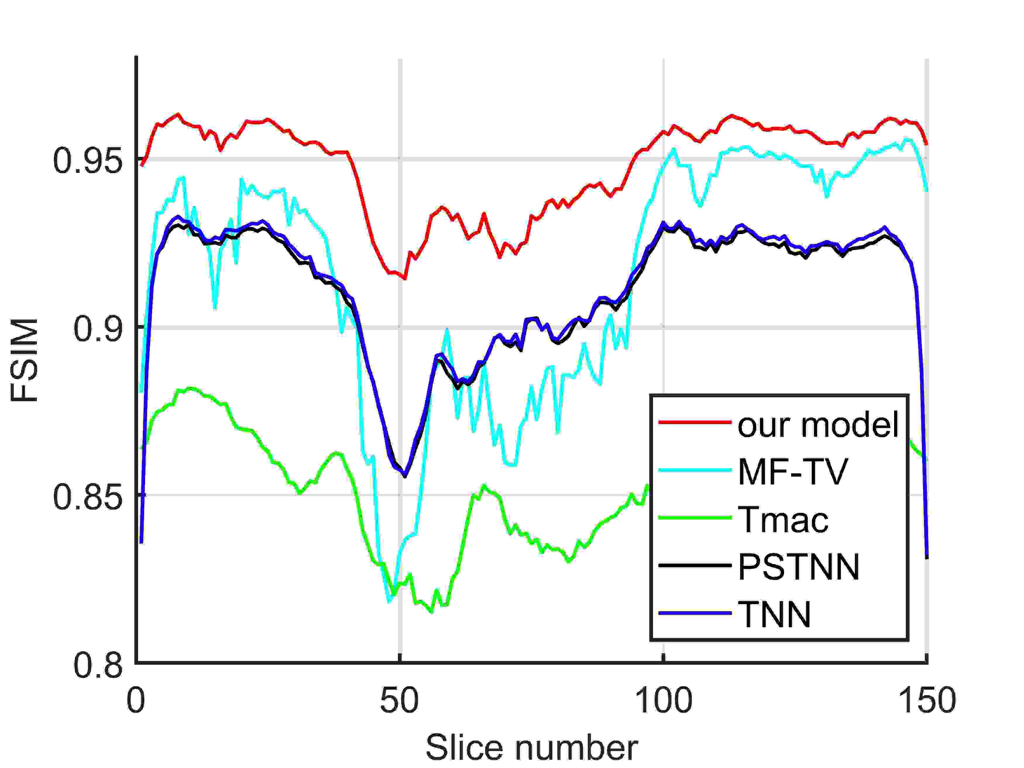
(i)

Figure 8: The PSNR, SSIM and FSIM of the recovered video ”suzie” by MF-TV, Tmac, TNN, PSTNN and our model for all slices, respectively.

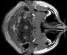
(a) Original

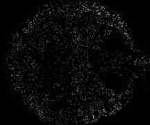
(b) 90% Masked

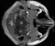
(c) our model

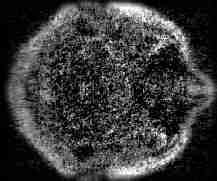
(d) MF-TV

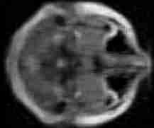
(e) Tmac

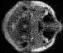
(f) PSTNN

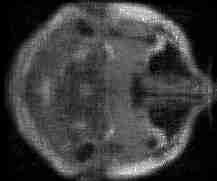
(g) TNN

Figure 9: One slice of the recovered MRI by our model, MF-TV, Tmac, PSTNN and TNN. The sampling rate is 10%.

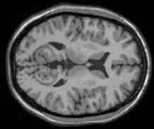
(a) Original

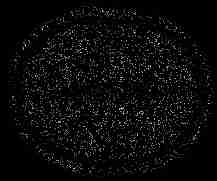
(b) 90% Masked

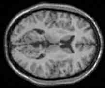
(c) our model

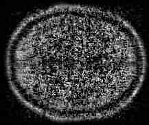
(d) MF-TV

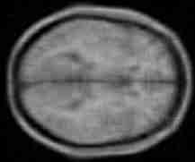
(e) Tmac

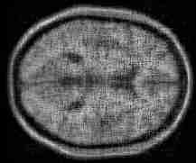
(f) PSTNN

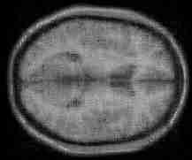
(g) TNN

Figure 10: One slice of the recovered MRI by our model, MF-TV, Tmac, PSTNN and TNN. The sampling rate is 10%.

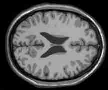
(a) Original

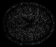
(b) 90% Masked

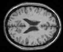
(c) our model

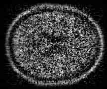
(d) MF-TV

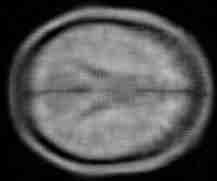
(e) Tmac

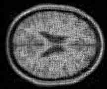
(f) PSTNN

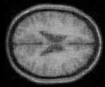
(g) TNN

Figure 11: One slice of the recovered MRI by our model, MF-TV, Tmac, PSTNN and TNN. The sampling rate is 10%.

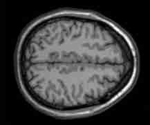
(a) Original

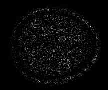
(b) 90% Masked

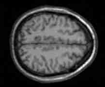
(c) our model

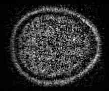
(d) MF-TV

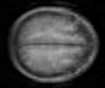
(e) Tmac

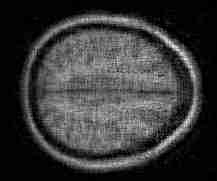
(f) PSTNN

(g) TNN

Figure 12: One slice of the recovered MRI by our model, MF-TV, Tmac, PSTNN and TNN. The sampling rate is 10%.

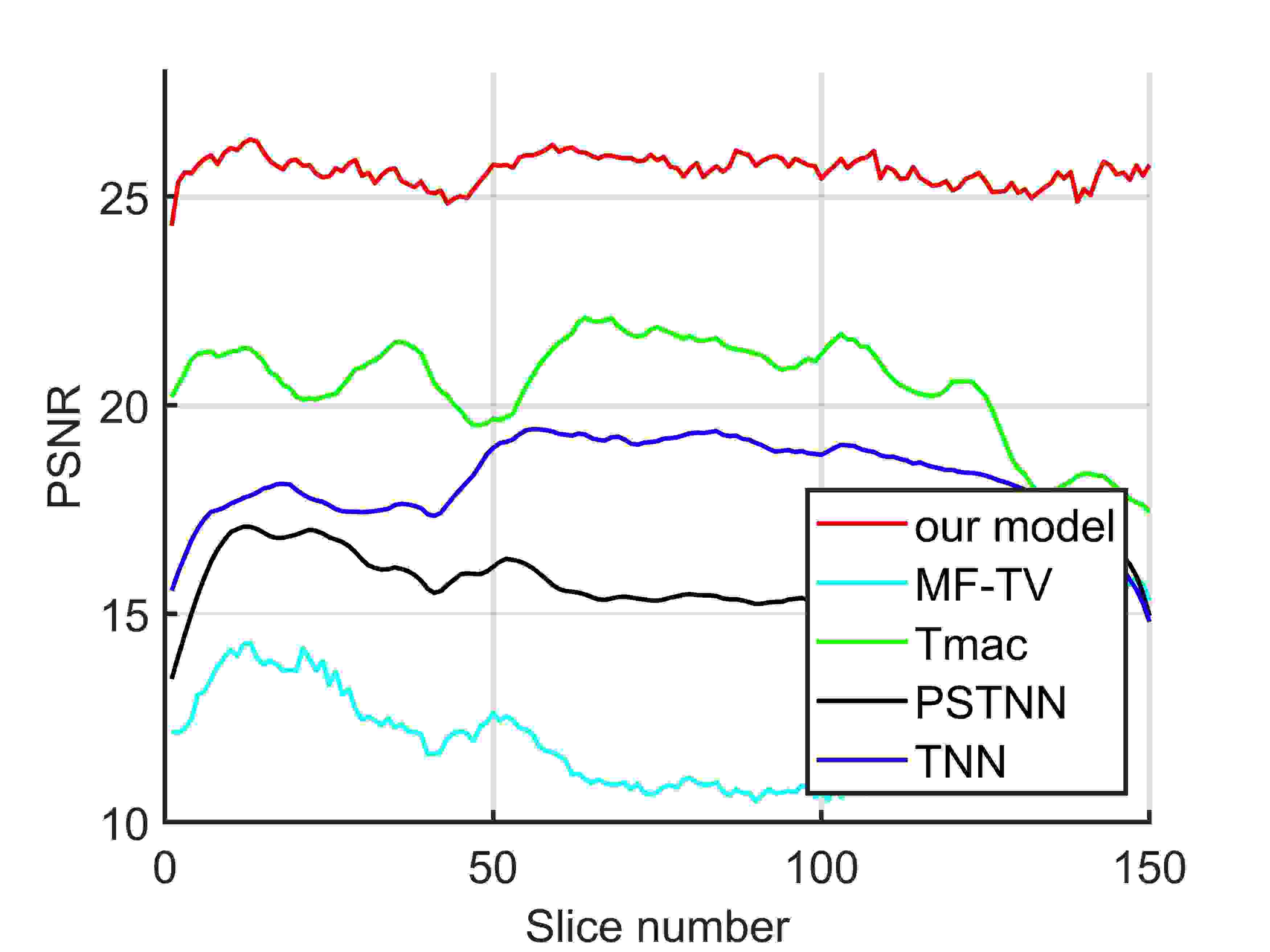
(a)

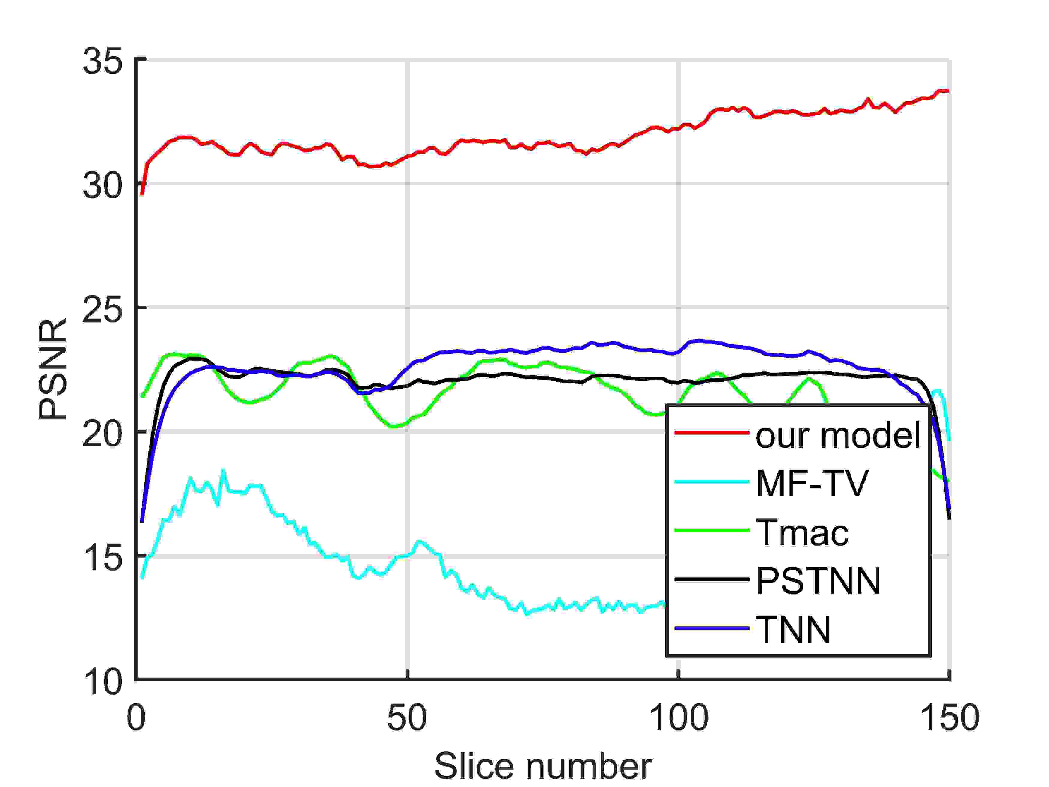
(b)

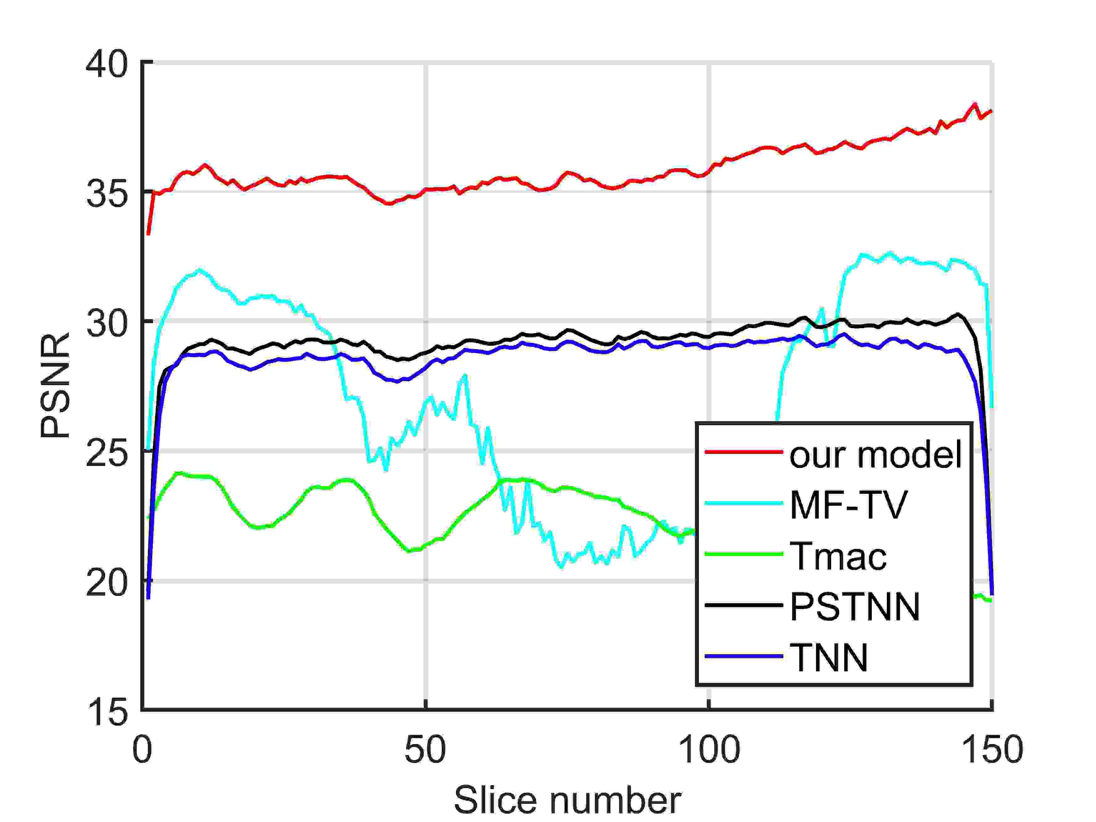
(c)

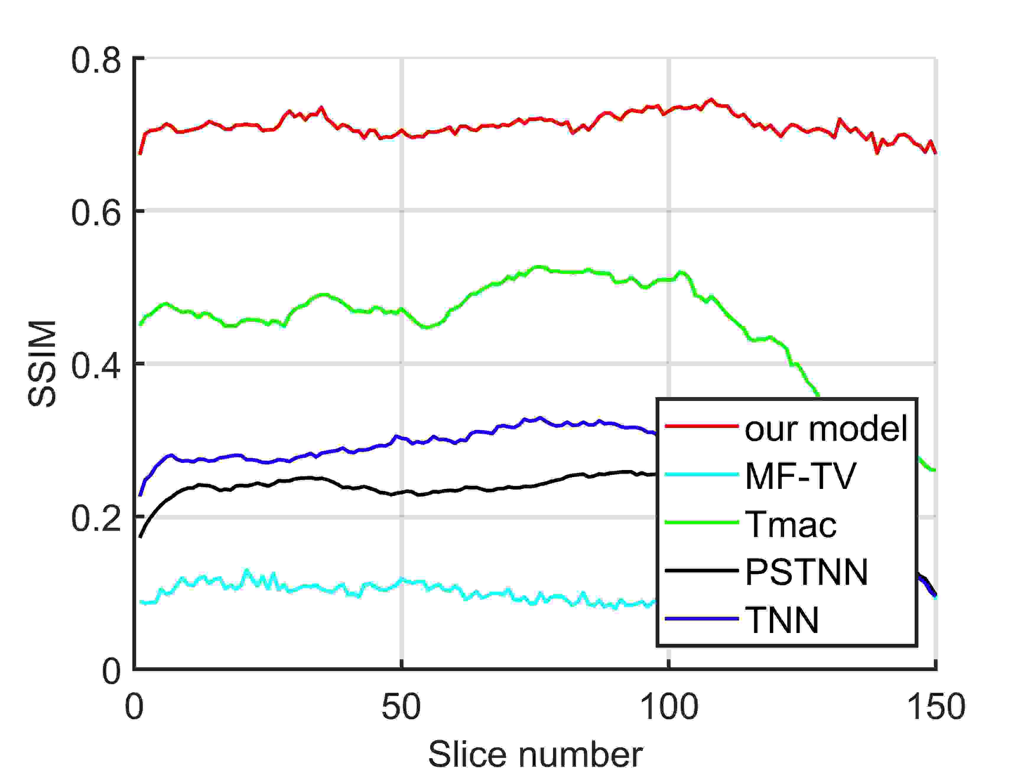
(d)

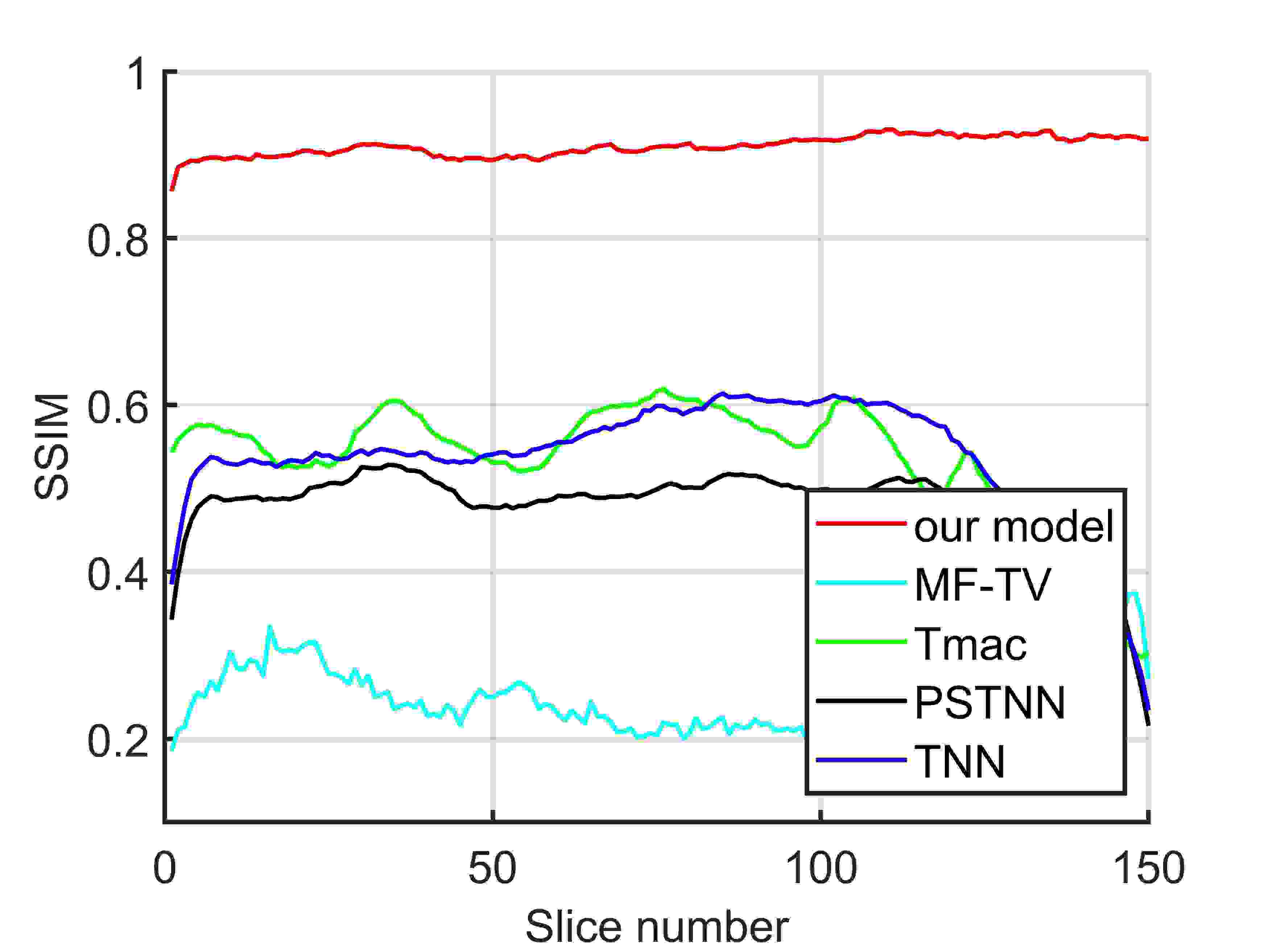
(e)

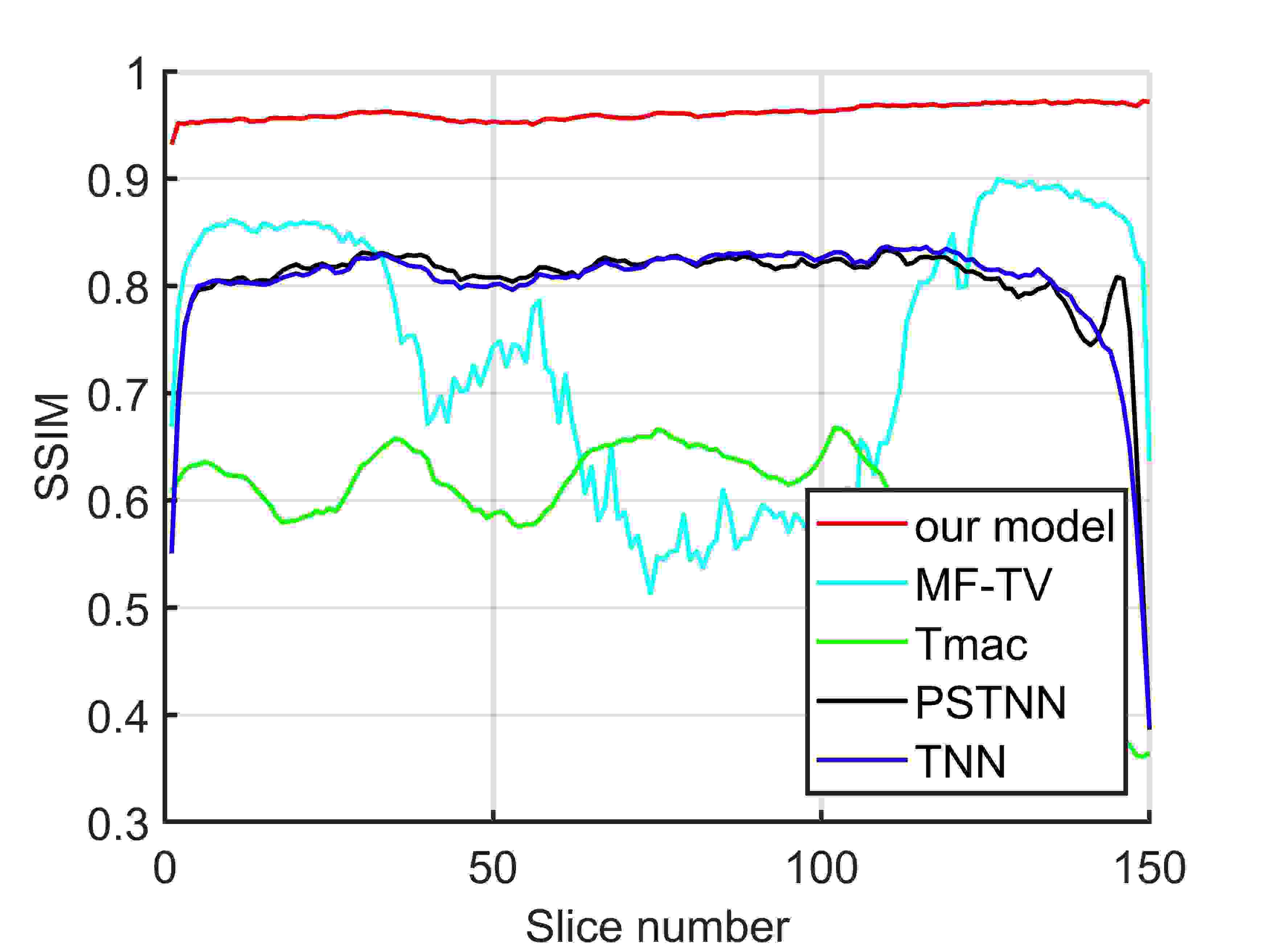
(f)

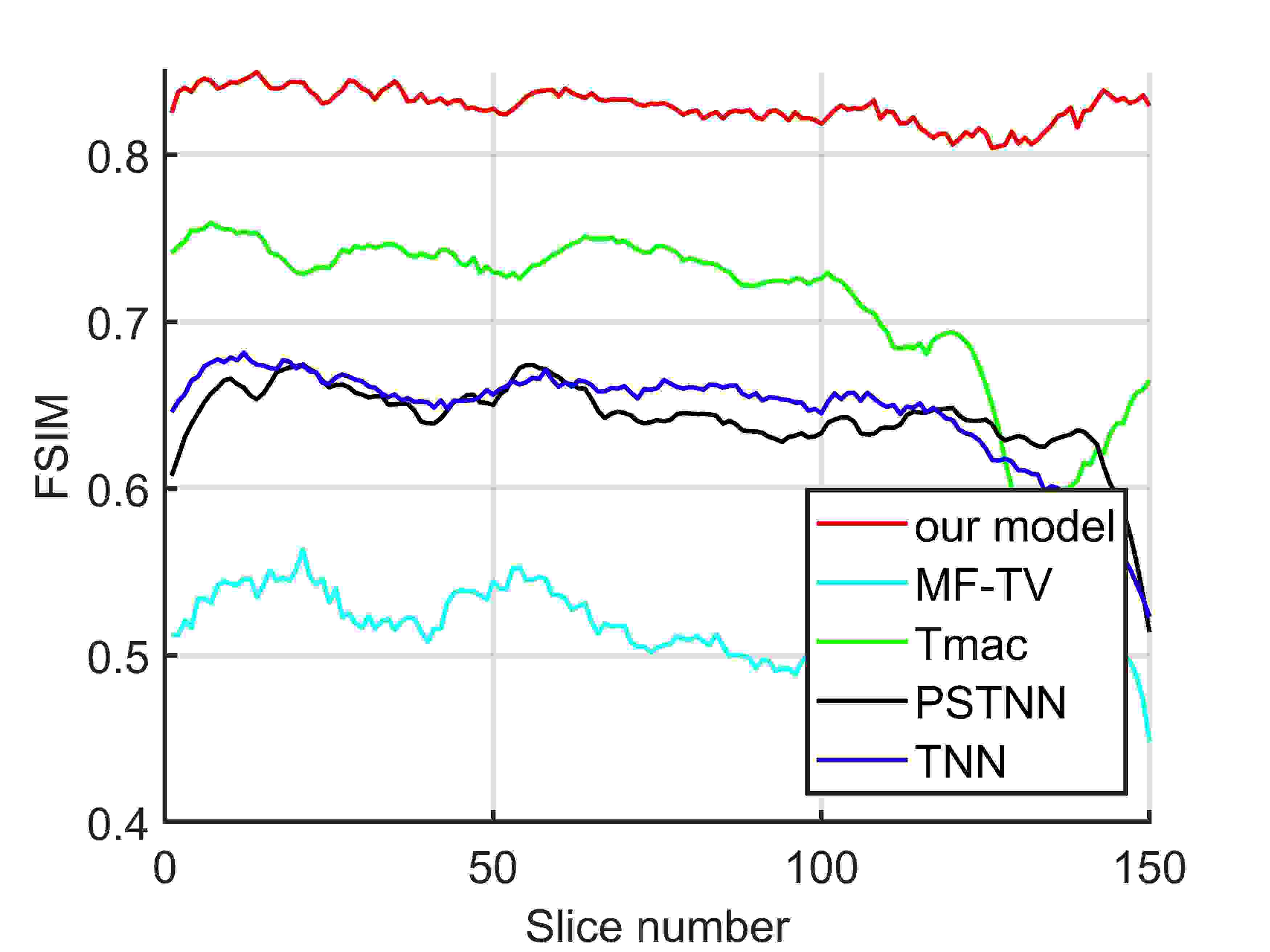
(g)

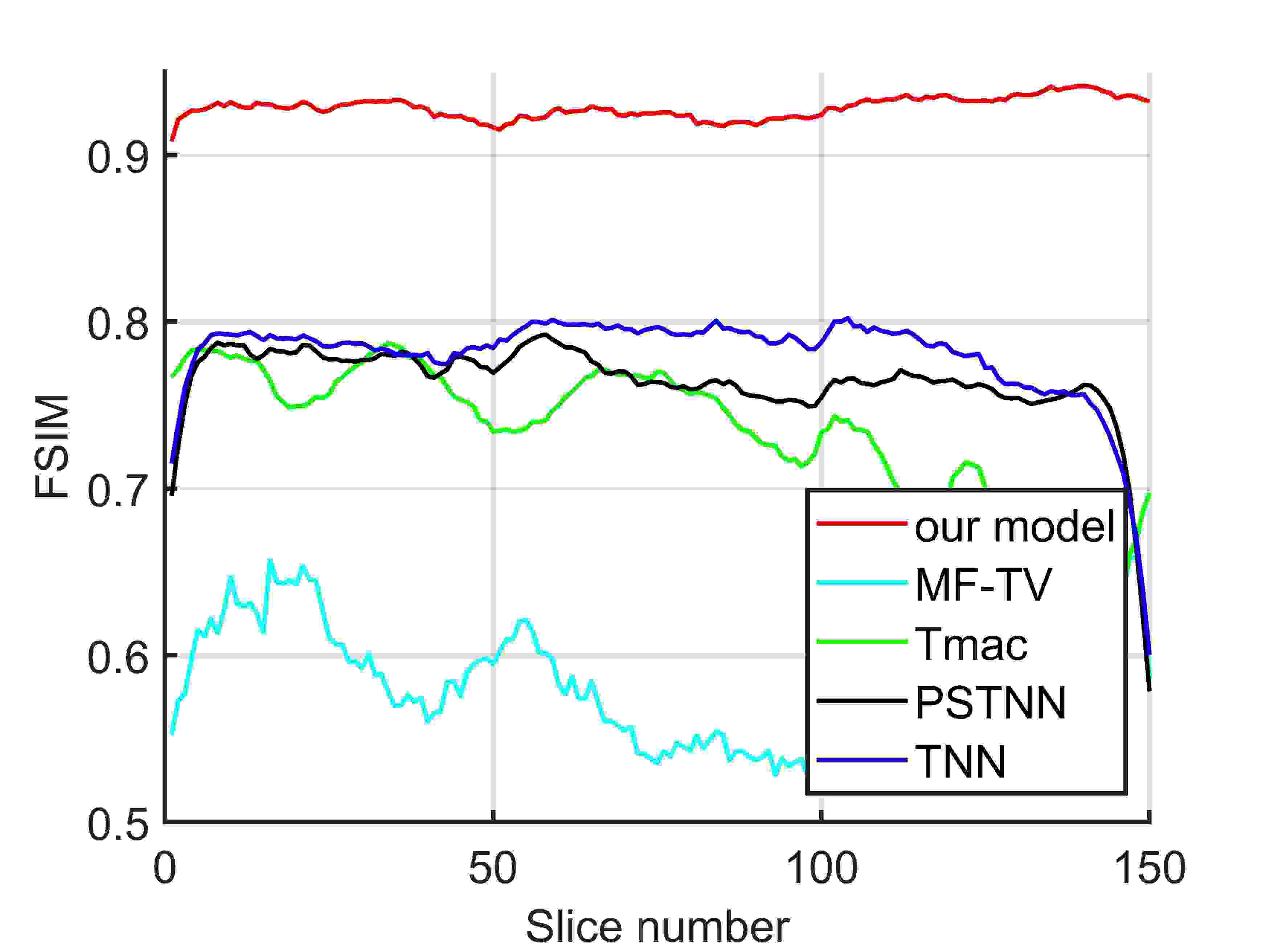
(h)

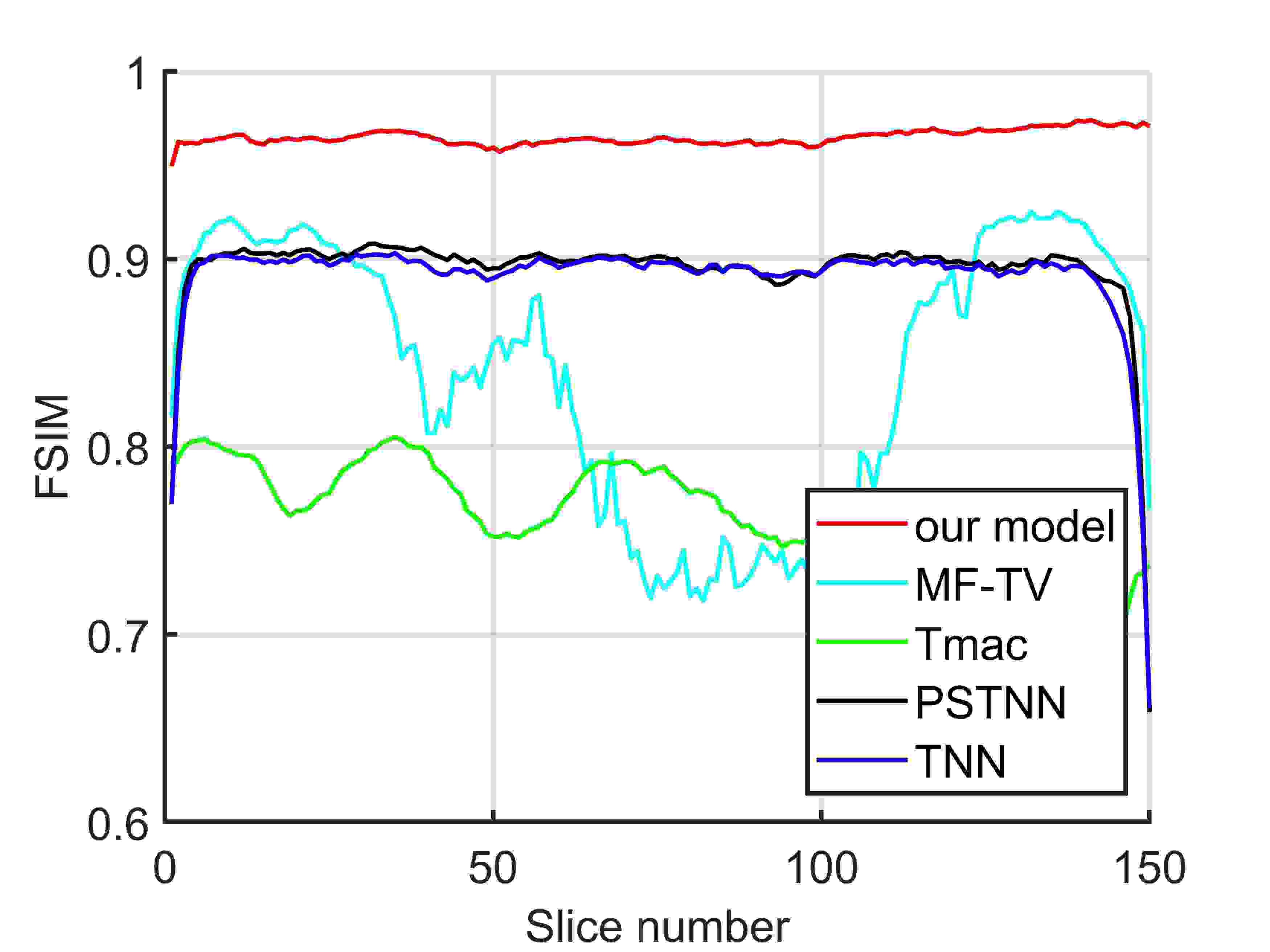
(i)

Figure 13: The PSNR, SSIM and FSIM of the recovered MRI by MF-TV, Tmac, TNN, PSTNN and our model for all slices, respectively.

To further verify the versatility of our model for different datasets, in this subsection we compare our model with MF-TV, Tmac, TNN and PSTNN on MRI dataset, i.e., the cubical MRI data. Its one slice is shown in Fig. 9. The size of the dataset is 181 $\times$ 217 $\times$ 150. We test all five methods on a series of sampling rates: 5%, 10%, 20% and 30%. In addition, the $n$-rank is approximated by using the number of the largest 0.5% singular values.

For quantitative comparison, Table III reports the PQIs of the results completed by different methods. The best result for each PQI are marked in bold. From Table III, it can be found that our method obtains the highest indices among the five tested methods in all SR cases. Further, the same advantage of our model can also be seen in Fig. 13 which reports the PSNR, SSIM and FSIM of each slice.

For visual comparison, Fig. 9, Fig. 10, Fig. 11 and Fig. 12 show slices with 90% missing values and the corresponding completed slices by all the tested methods. From the results, we see again that our model can better retain the local details and texture information of the images, and effectively restore the main structure of the images than other compared methods. Therefore, one can see that the recovered data obtained by our model has the best visual evaluation.

TABLE III: The averaged PSNR, SSIM, FSIM, ERGA and SAM of the recovered results on MRI by Tmac, MF-TV, TNN, PSTNN and our model with different sampling rates. The best values are highlighted in bolder fonts.

			SR =0.05
PQI	nosiy	our model	MF-TV	TMac	PSTNN	TNN
PSNR	10.258	26.414	12.332	20.51	15.859	18.218
SSIM	0.228	0.722	0.099	0.45	0.224	0.27
FSIM	0.473	0.834	0.52	0.711	0.642	0.646
ERGA	1030.203	184.279	814.747	339.385	545.77	434.774
MSAM	76.54	20.411	55.603	31.367	36.355	31.11
			SR = 0.1
PQI	nosiy	our model	MF-TV	TMac	PSTNN	TNN
PSNR	10.492	32.652	15.406	21.411	22.061	22.535
SSIM	0.241	0.912	0.25	0.531	0.482	0.536
FSIM	0.511	0.926	0.587	0.732	0.764	0.78
ERGA	1002.8	89.116	584.827	308.655	275.473	266.753
MSAM	70.986	14.637	41.826	29.345	24.585	24.6
			SR = 0.2
PQI	nosiy	our model	MF-TV	TMac	PSTNN	TNN
PSNR	11.003	36.529	27.062	22.33	29.152	28.571
SSIM	0.271	0.962	0.737	0.586	0.804	0.802
FSIM	0.564	0.963	0.84	0.754	0.895	0.891
ERGA	945.583	57.037	173.636	276.269	127.133	136.182
MSAM	62.887	11.559	21.792	27.267	17.513	17.855

V-C Hyperspectral Image Data

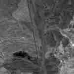
(a) Original

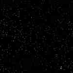
(b) 97.5% Masked

(c) our model

(d) MF-TV

(e) Tmac

(f) PSTNN

(g) TNN

Figure 14: One slice of the recovered HSI ”Cuprite” by our model, MF-TV, Tmac, PSTNN and TNN. The sampling rate is 2.5%.

(a) Original

(b) 95% Masked

(c) our model

(d) MF-TV

(e) Tmac

(f) PSTNN

(g) TNN

Figure 15: One slice of the recovered HSI ”Cuprite” by our model, MF-TV, Tmac, PSTNN and TNN. The sampling rate is 5%.

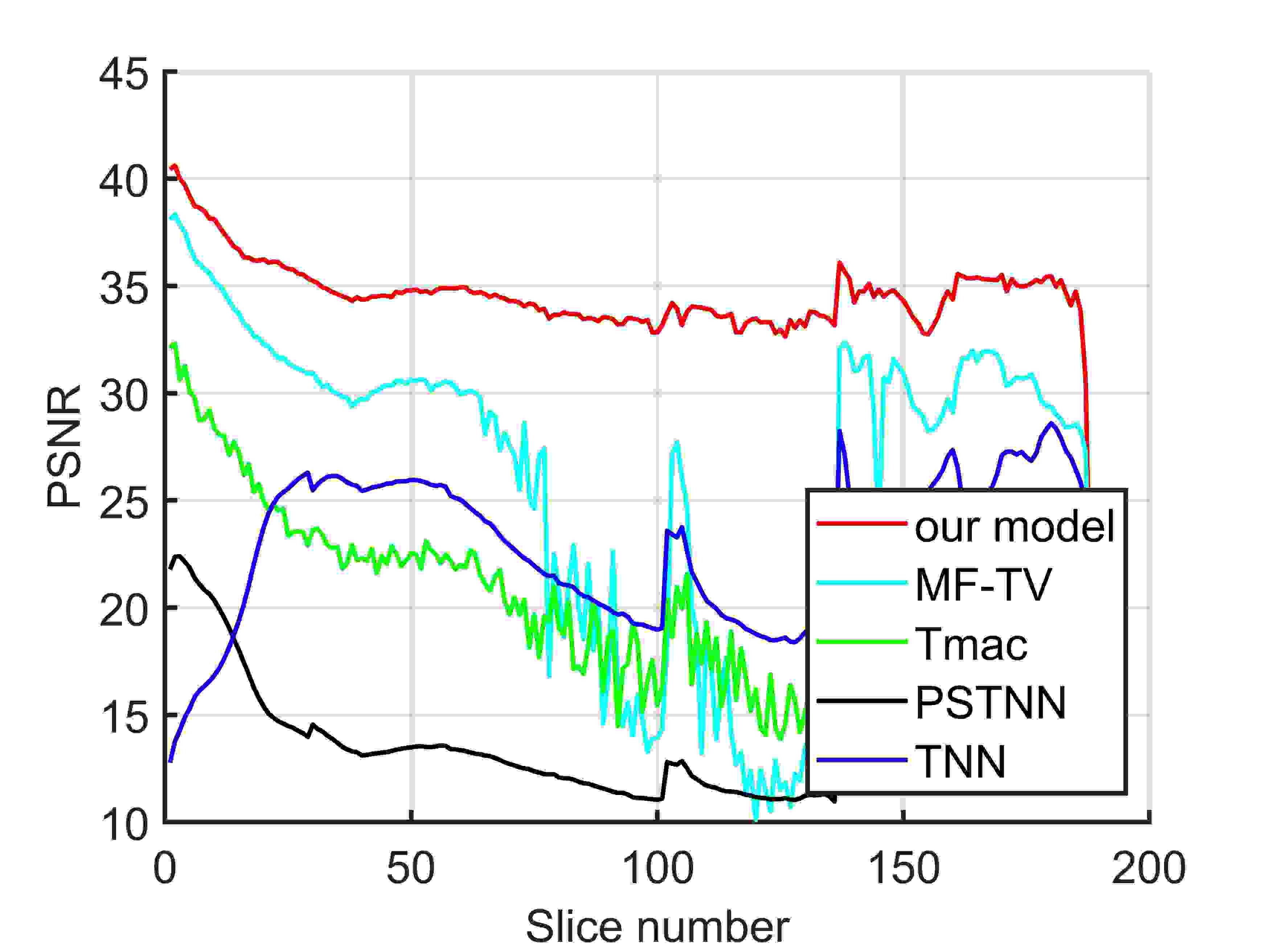
(a) PSNR

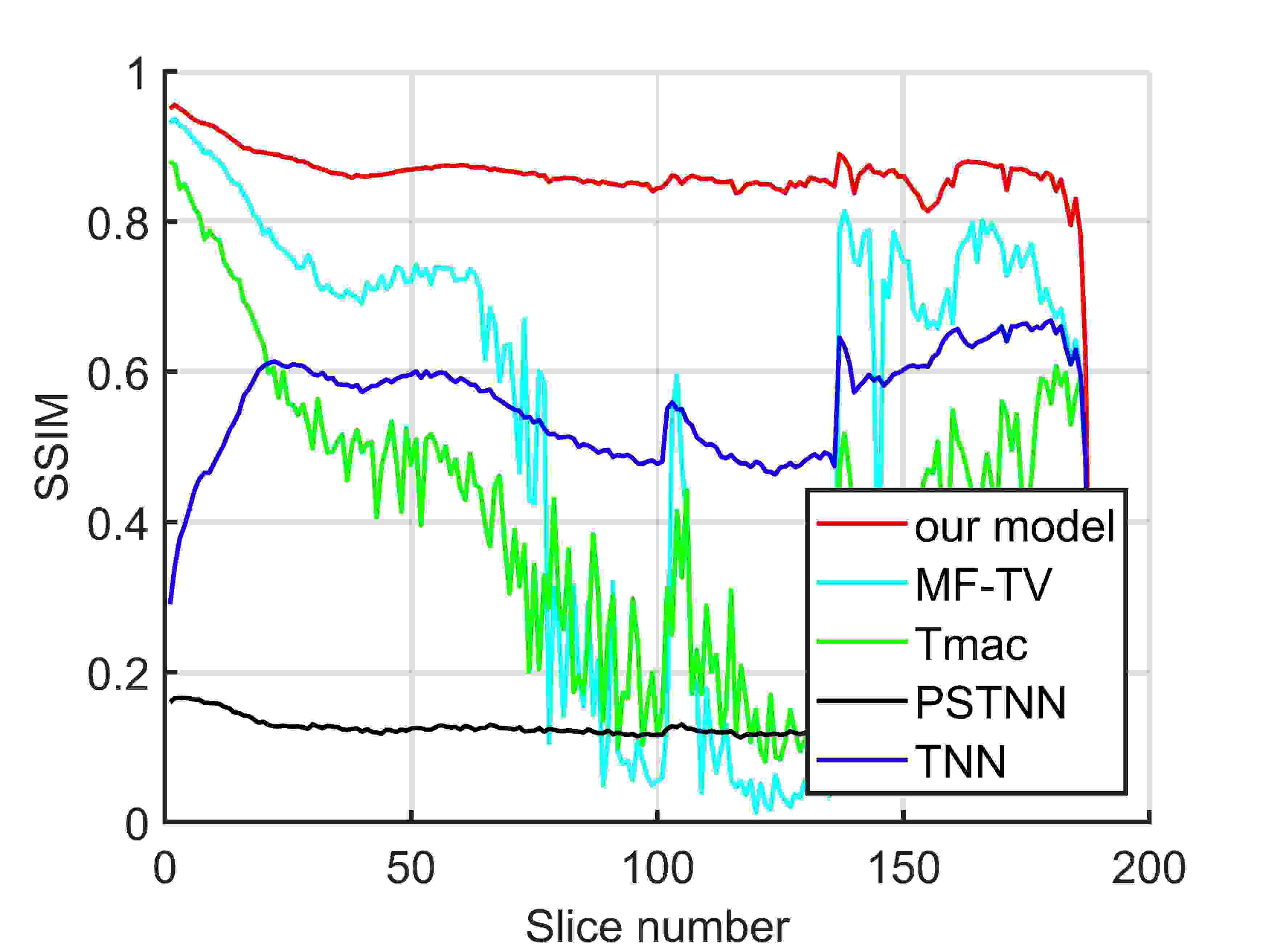
(b) SSIM

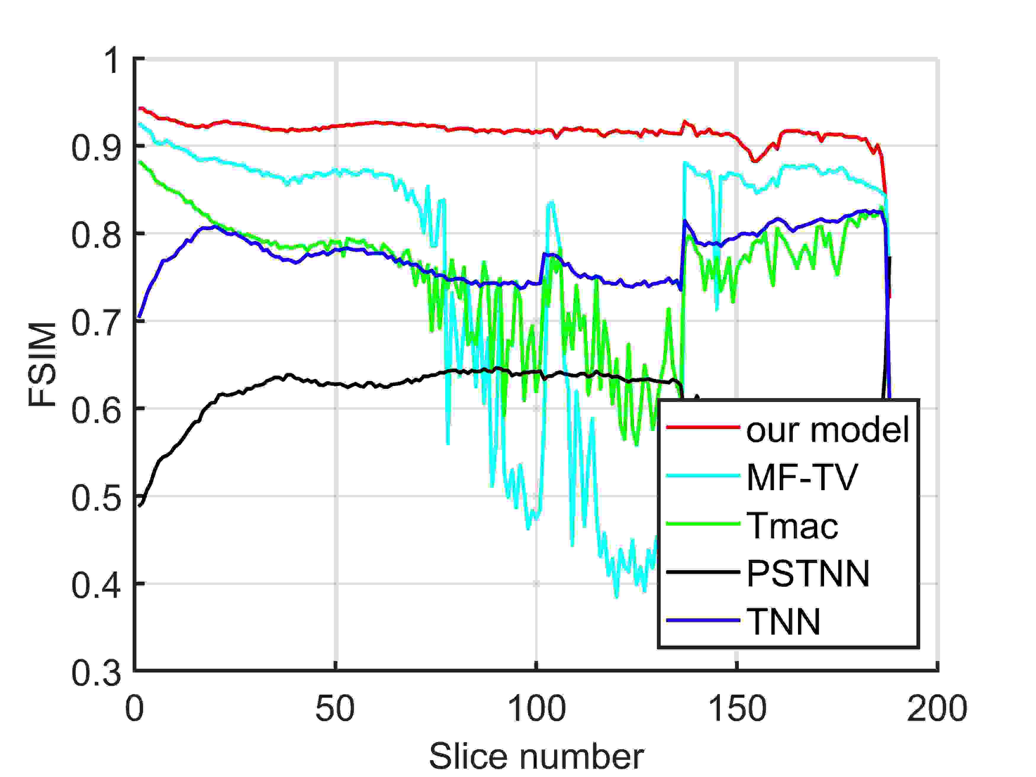
(c) FSIM

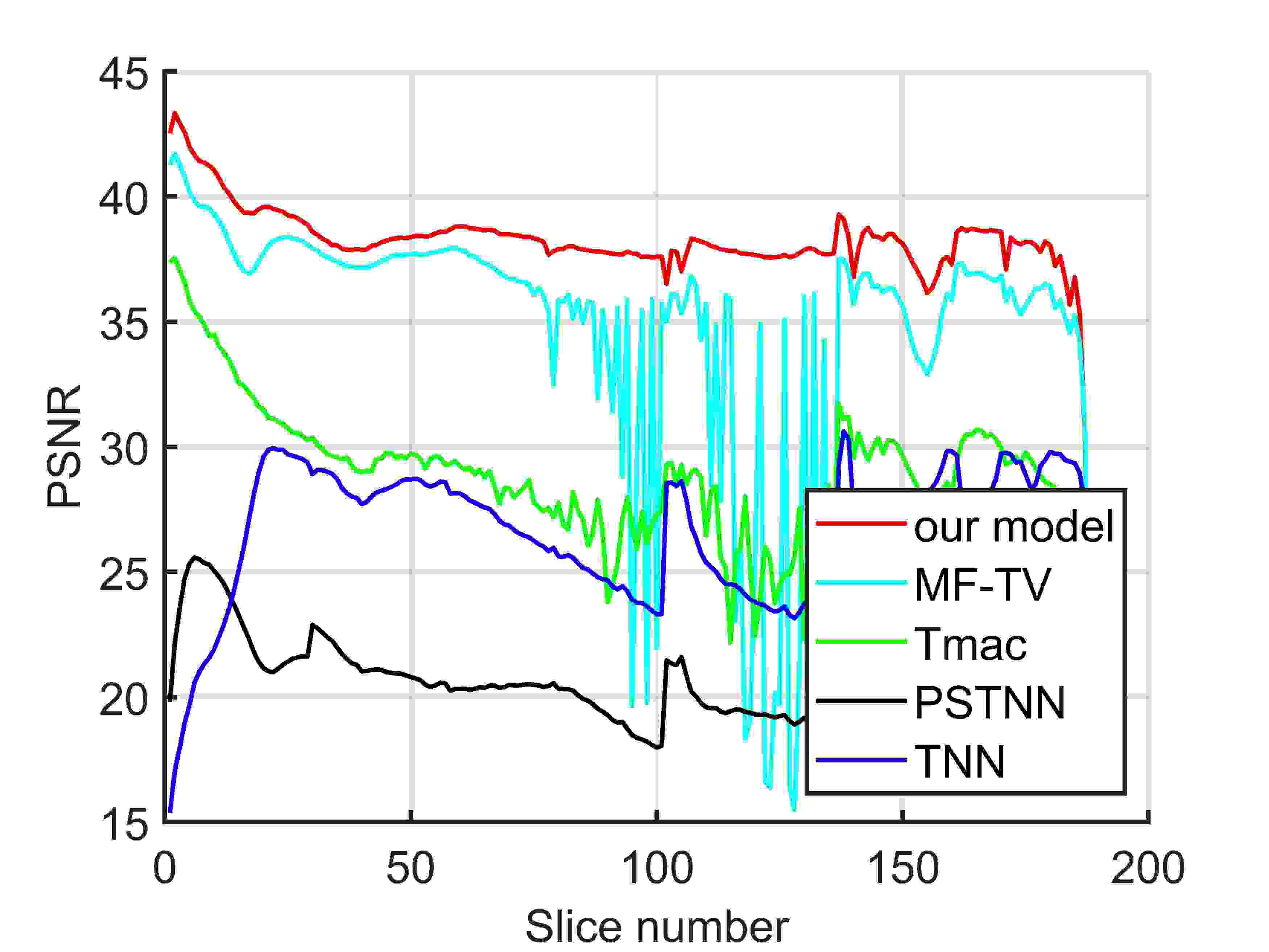
(d) PSNR

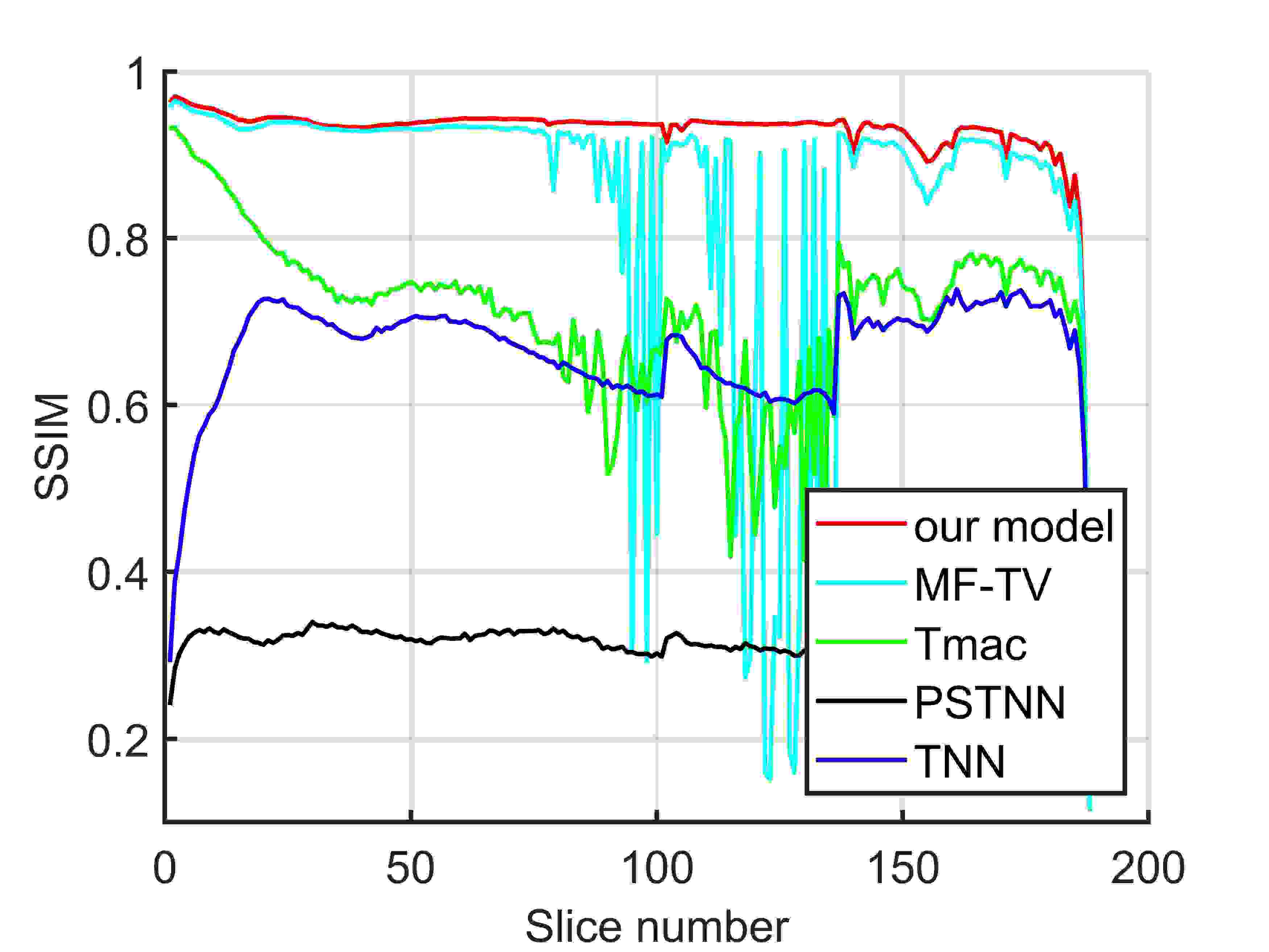
(e) SSIM

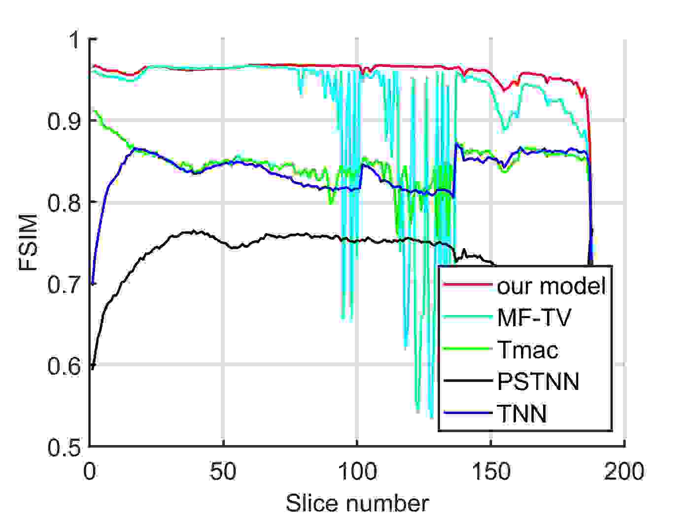
(f) FSIM

Figure 16: The PSNR, SSIM and FSIM of the recovered HSI ”Cuprite” by MF-TV, Tmac, TNN, PSTNN and our model for all slices, respectively.(a)-(c): 97.5% entries missing, (d)-(f): 95% entries missing.

In this section, we compare our model with MF-TV, Tmac, TNN and PSTNN on one HSI dataset: Airborne Visible/Infrared Imaging Spectrometer (AVIRIS) Cuprite data. The size of AVIRIS Cuprite data is 150 $\times$ 150 $\times$ 188. Its one slice is shown in Fig. 15. We test all five methods on a series of sampling rates: 2.5%, 5% and 10%. In addition, the $n$-rank is approximated by using the number of the largest 0.3% singular values.

For quantitative comparison, Table IV reports the average PQIs of each tested method with three different sampling rates. At sampling rates 0.025 and 0.05, Fig. 16 reports the PSNR, SSIM and FSIM of each frontal slice in the completed results. For visual comparison, Fig. 15 and Fig. 14 show slices of the sampled data with 97.5% and 95% missing values and the corresponding recovered slices by the tested methods. From the results, we see again that our model not only obtains the highest PQIs, but also recovers more structure information and spatial details of the images than compared methods, especially at low sampling rates.

TABLE IV: The averaged PSNR, SSIM, FSIM, ERGA and SAM of the recovered results on hyperspectral image ”Cuprite” by Tmac, MF-TV, TNN, PSTNN and our model with different sampling rates. The best values are highlighted in bolder fonts.

			SR =0.025
PQI	nosiy	our model	MF-TV	TMac	PSTNN	TNN
PSNR	7.666	34.595	26.115	21.25	13.387	22.783
SSIM	0.007	0.861	0.539	0.412	0.124	0.554
FSIM	0.48	0.916	0.765	0.755	0.613	0.775
ERGA	1043.633	50.383	237.074	235.594	539.574	245.333
MSAM	81.221	1.662	12.913	7.842	17.98	9.156
			SR = 0.05
PQI	nosiy	our model	MF-TV	TMac	PSTNN	TNN
PSNR	7.779	38.202	34.684	28.945	20.621	26.579
SSIM	0.01	0.928	0.845	0.712	0.31	0.663
FSIM	0.471	0.960	0.915	0.846	0.735	0.836
ERGA	1030.139	41.898	89.372	93.352	234.445	154.292
MSAM	77.268	1.559	4.386	3.278	7.886	5.413
			SR = 0.1
PQI	nosiy	our model	MF-TV	TMac	PSTNN	TNN
PSNR	8.013	39.056	40.888	35.627	35.51	35.015
SSIM	0.014	0.939	0.957	0.885	0.907	0.897
FSIM	0.451	0.966	0.978	0.931	0.951	0.943
ERGA	1002.75	34.544	34.263	44.518	54.421	57.537
MSAM	71.695	1.299	1.46	1.445	2.072	2.192

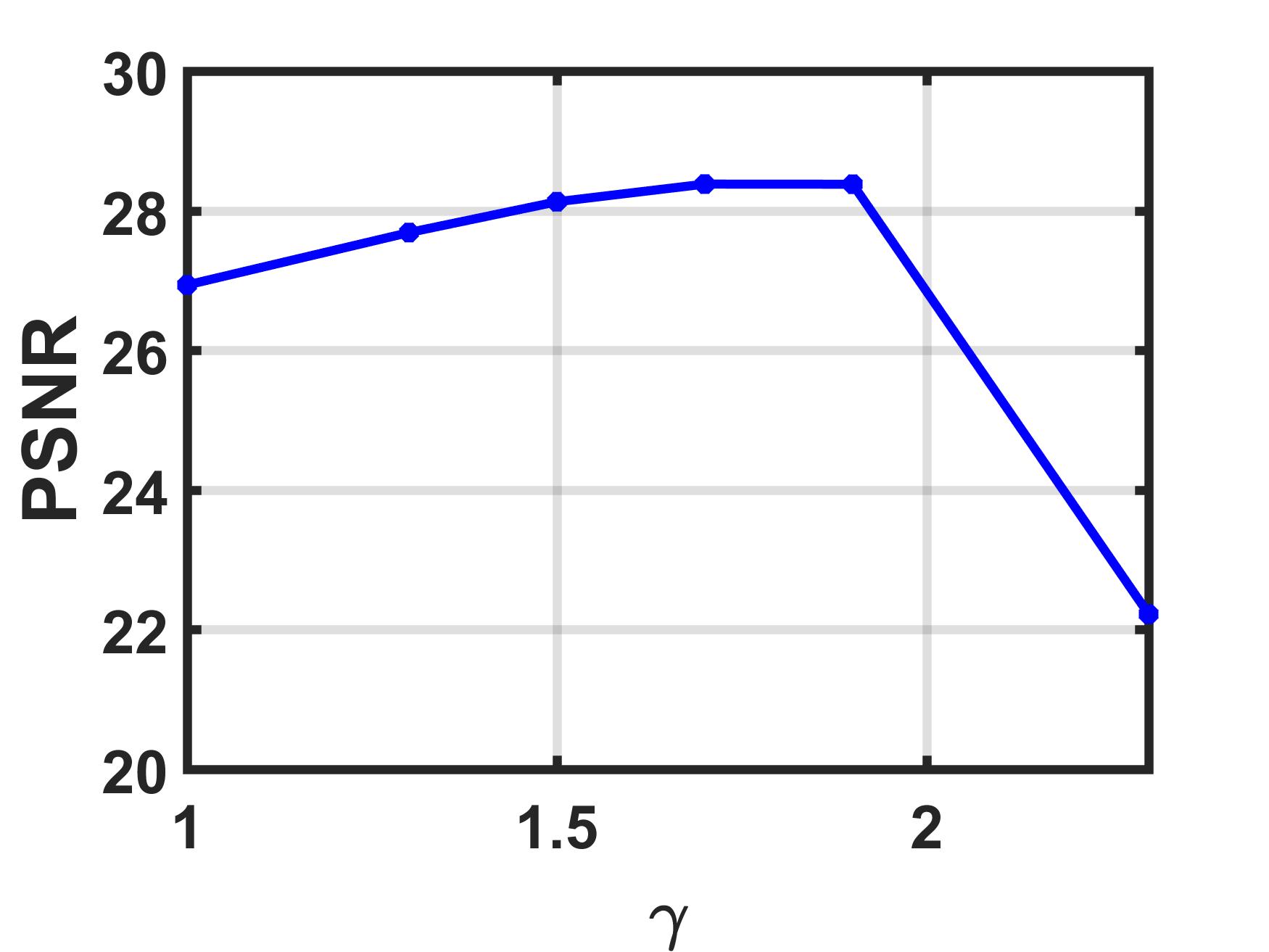
(a)

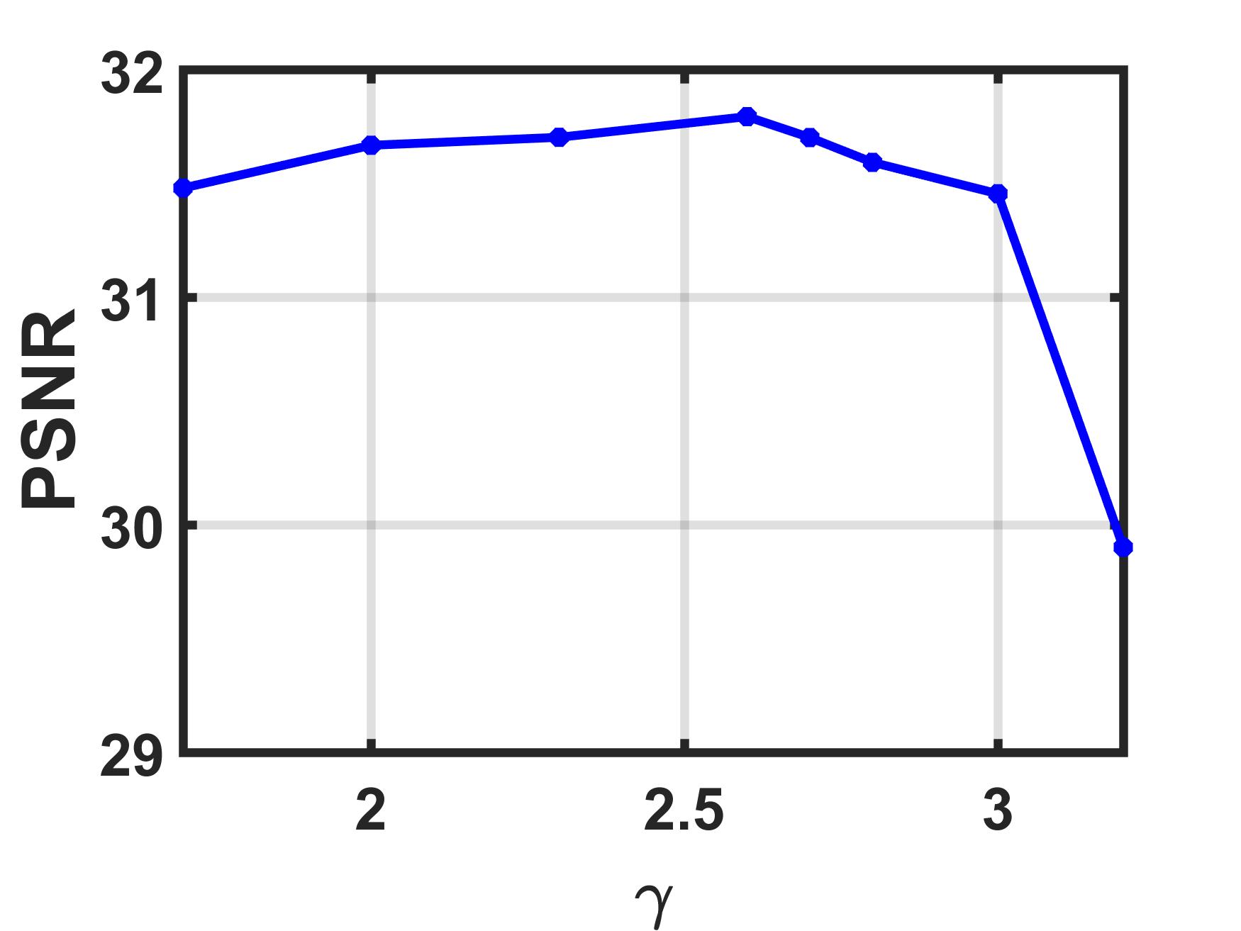
(b)

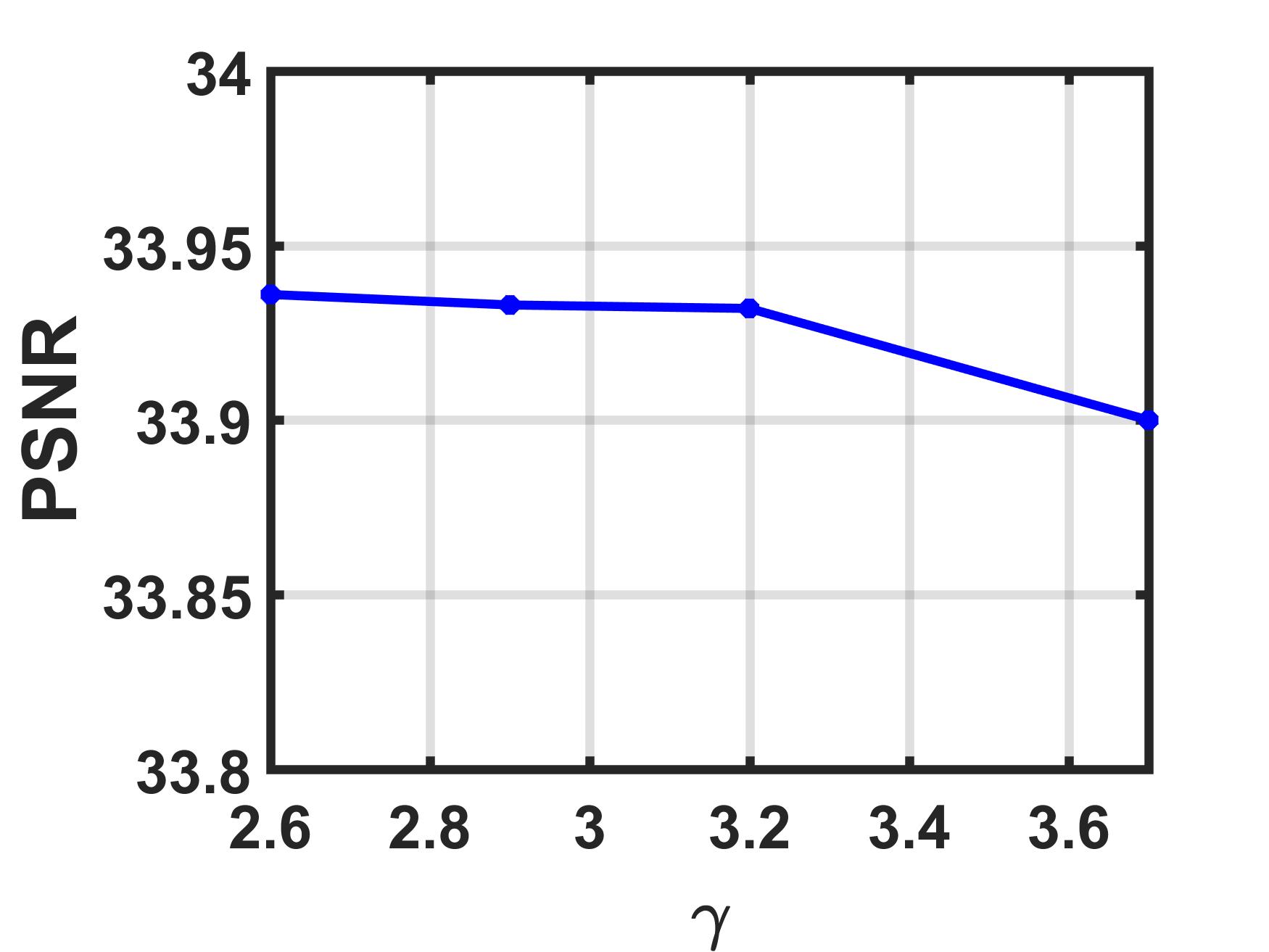
(c)

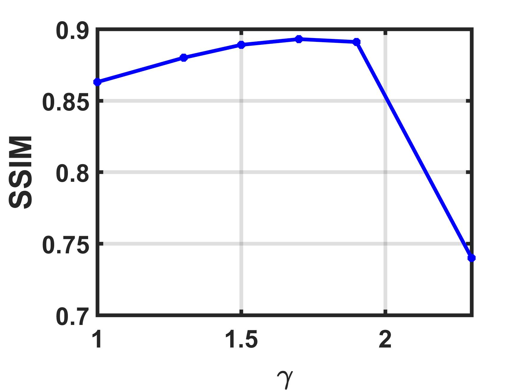
(d)

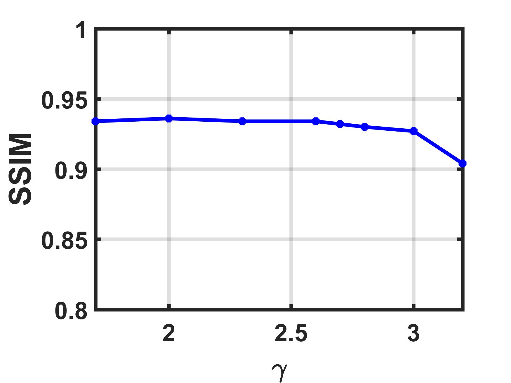
(e)

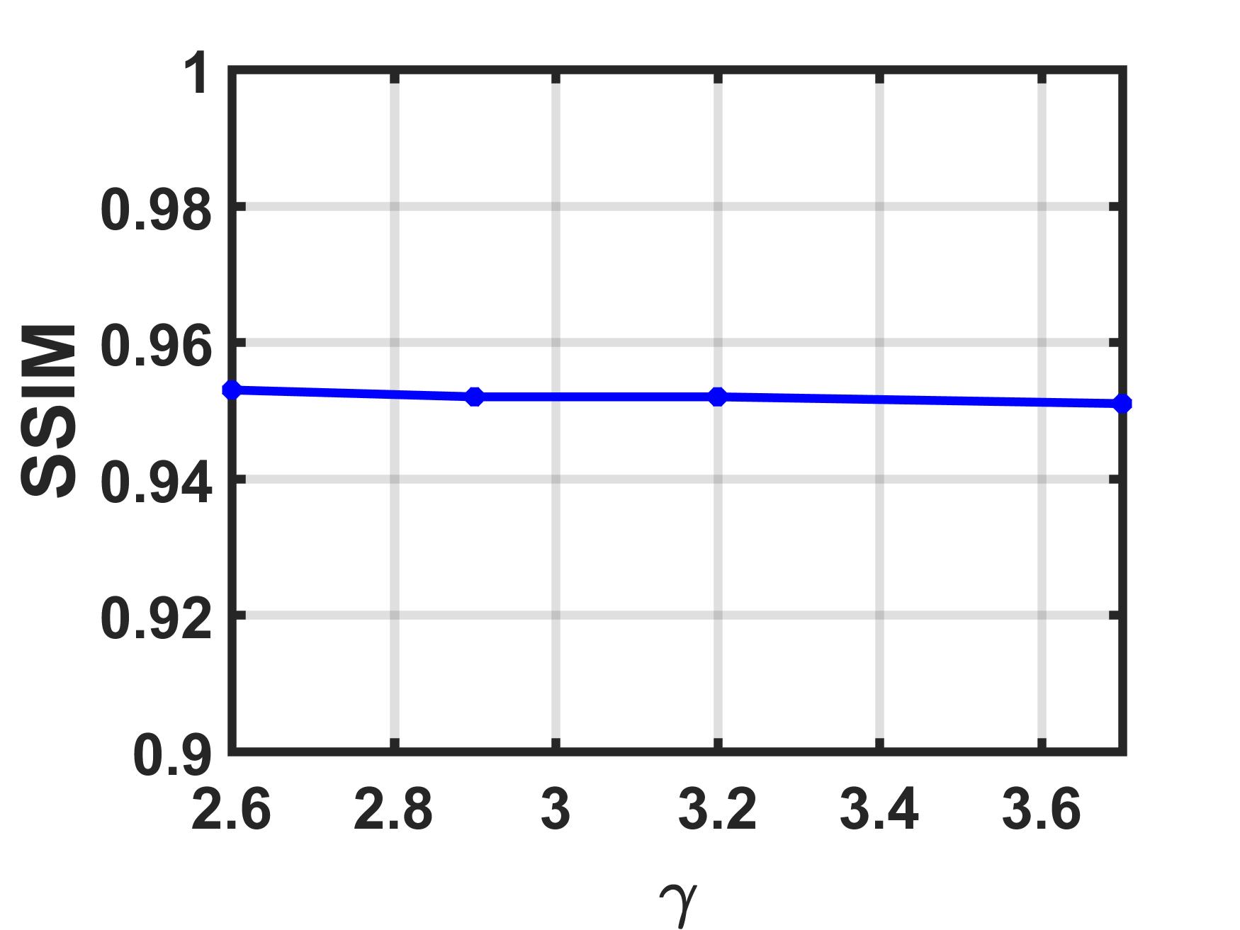
(f)

Figure 17: Sensitivity analysis of parameter $\gamma$ in video ”hall” dataset. (a-c) Change in the MPSNR value: SR= 0.05, 0.1 and 0.2. (e-f) Change in the MSSIM value: 0.05, 0.1 and 0.2, respectively.

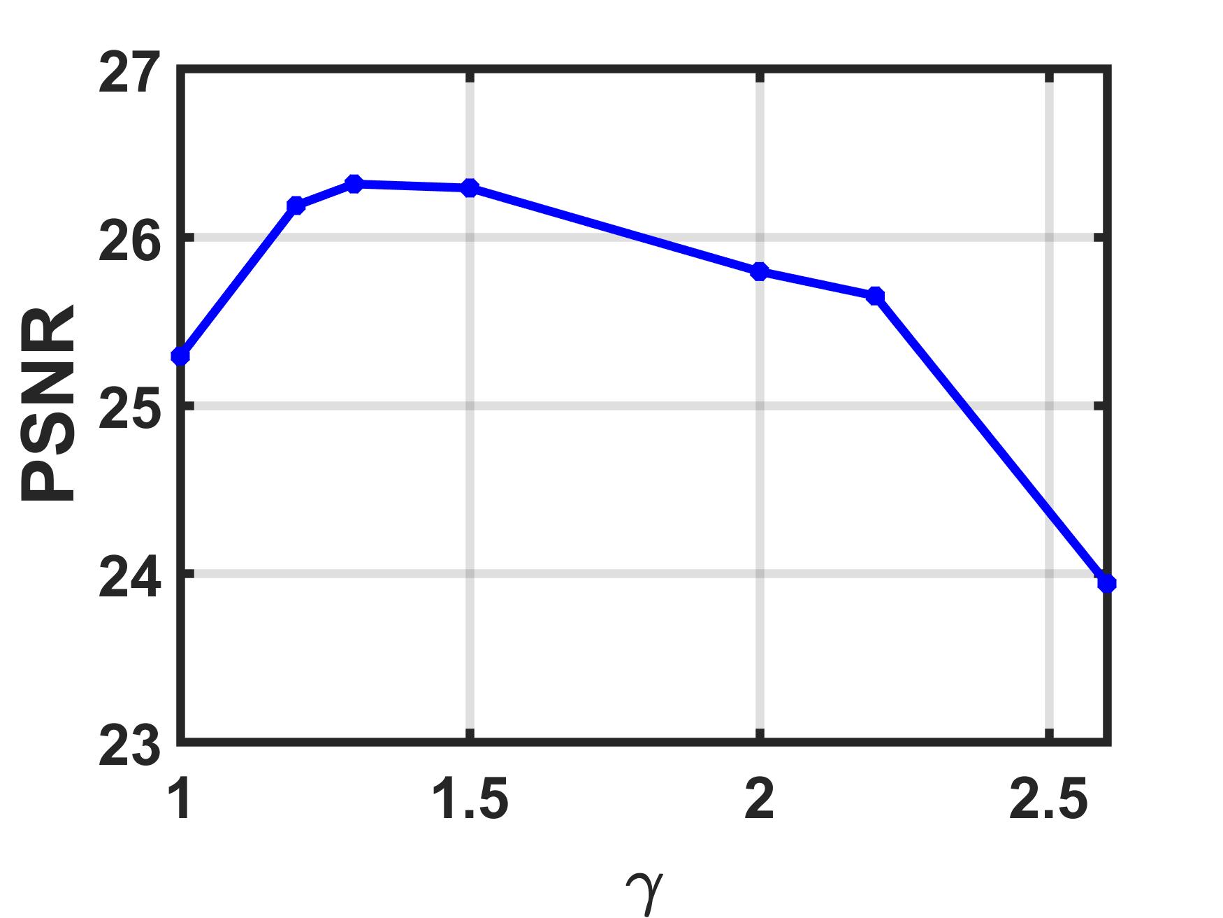
(a)

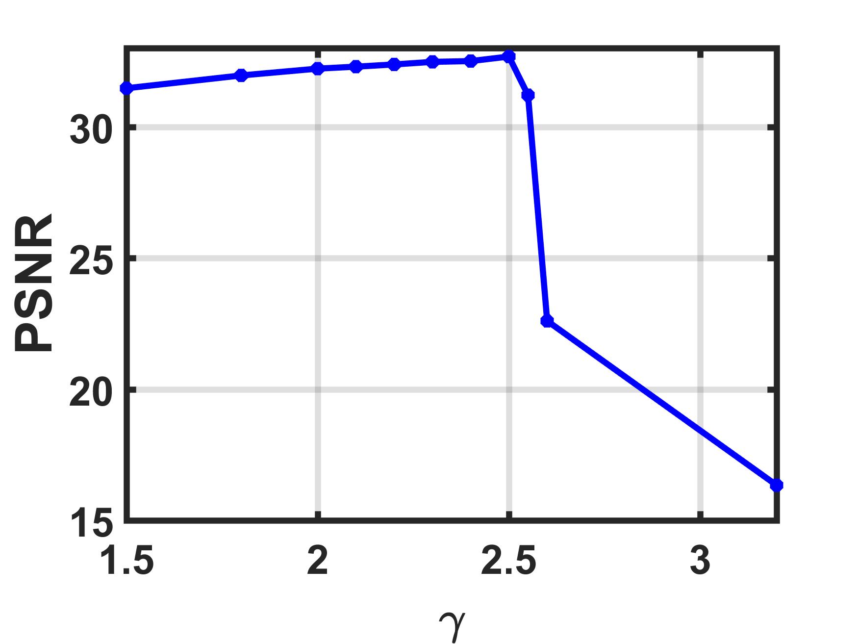
(b)

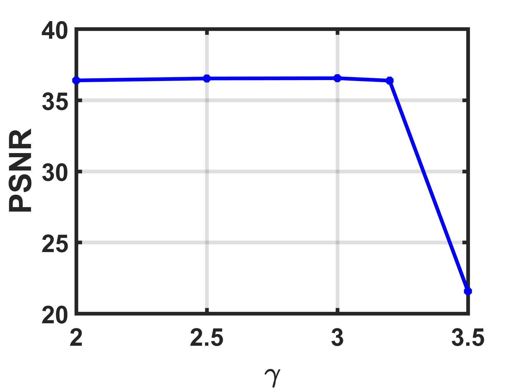
(c)

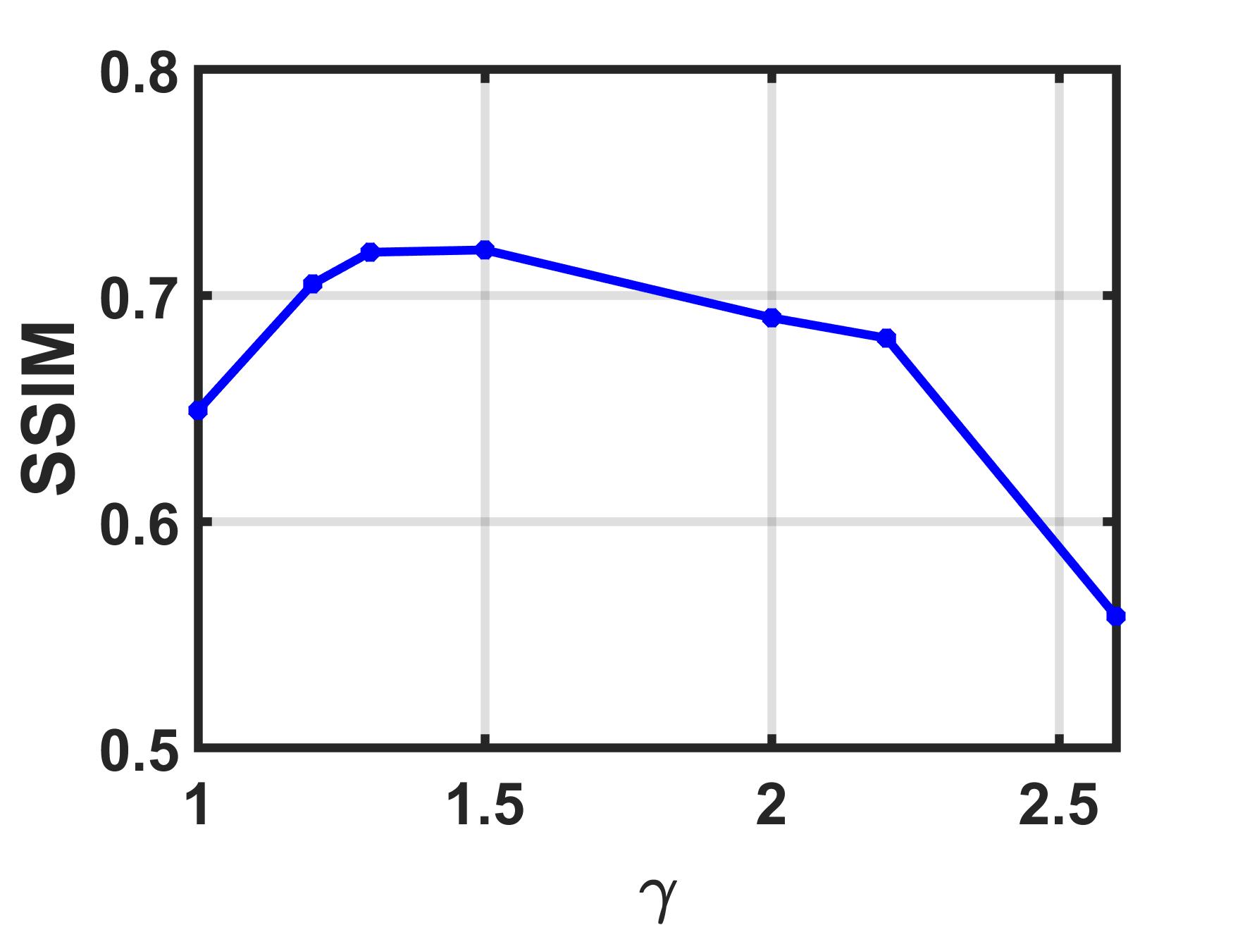
(d)

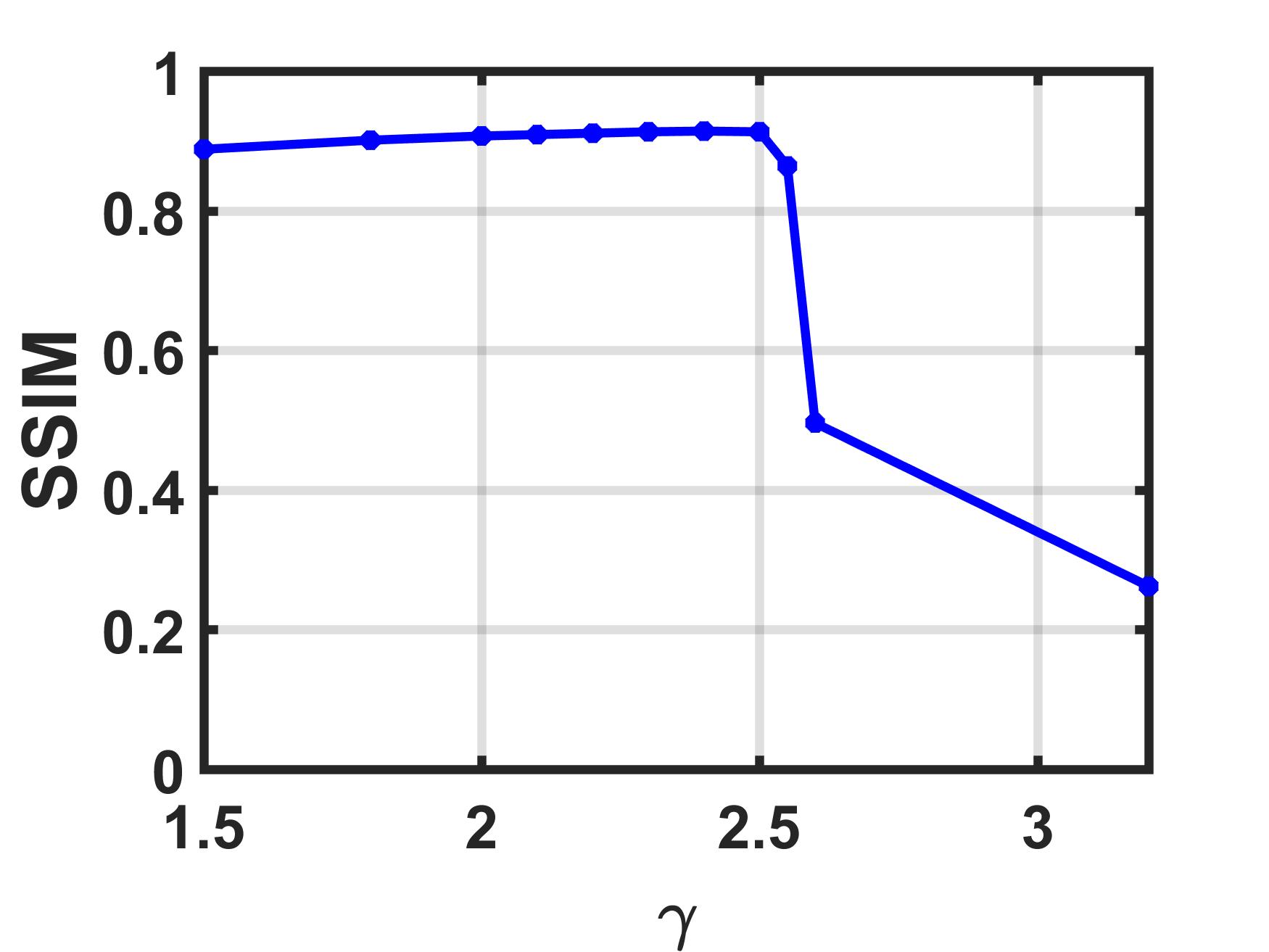
(e)

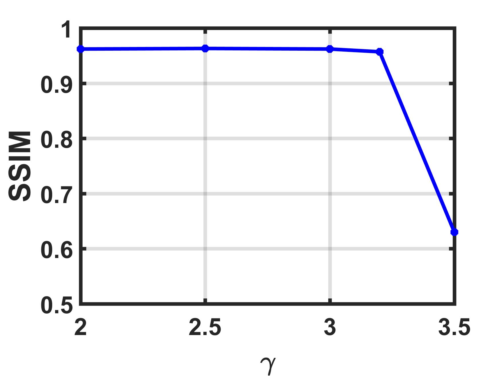
(f)

Figure 18: Sensitivity analysis of parameter $\gamma$ in MRI dataset. (a-c) Change in the MPSNR value: SR= 0.05, 0.1 and 0.2. (e-f) Change in the MSSIM value: 0.05, 0.1 and 0.2, respectively.

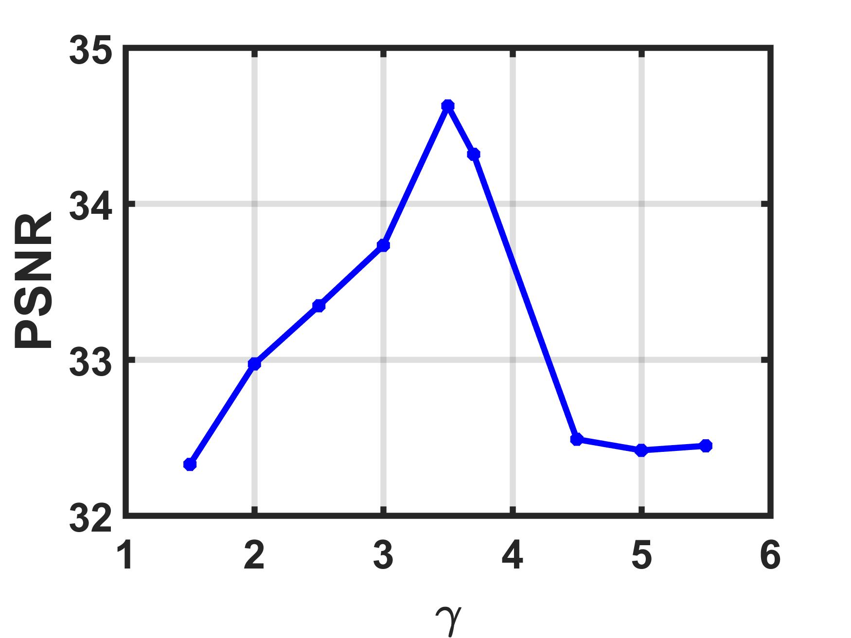
(a) SR=0.025

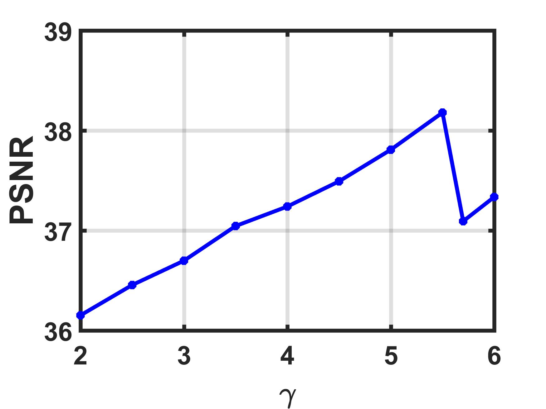
(b) SR=0.05

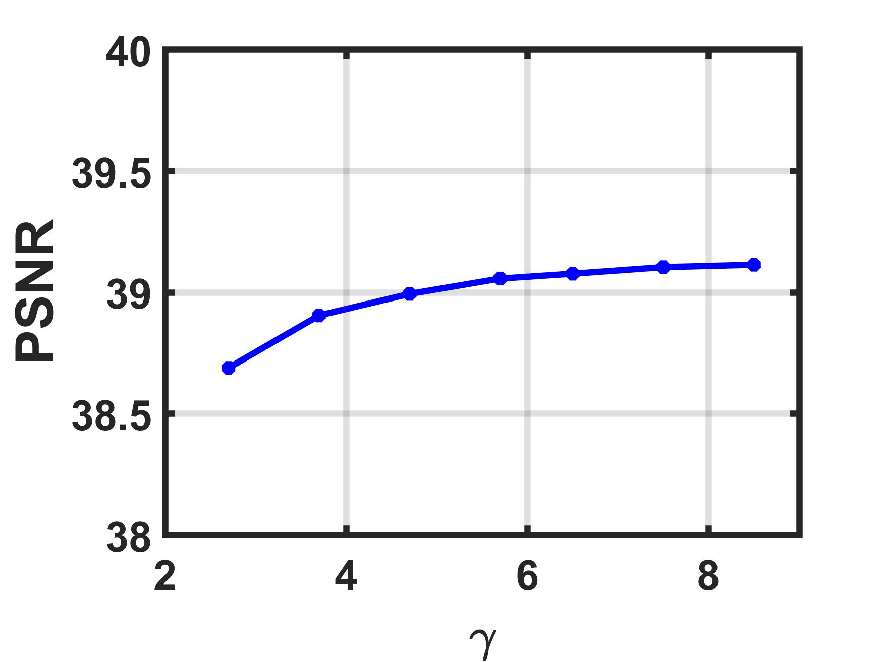
(c) SR=0.1

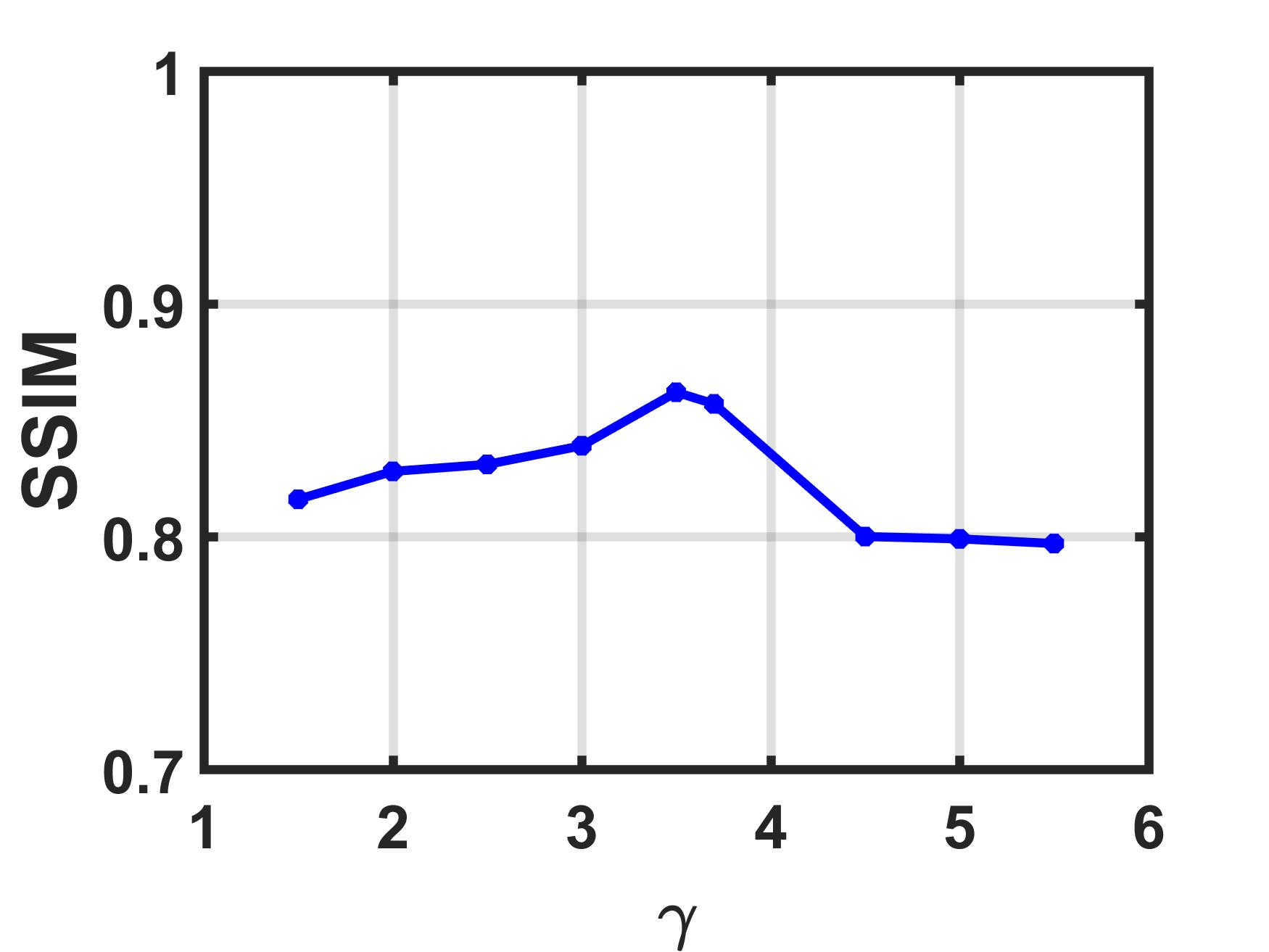
(d) SR=0.025

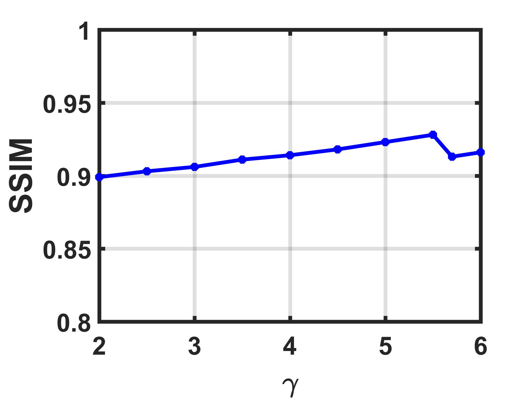
(e) SR=0.05

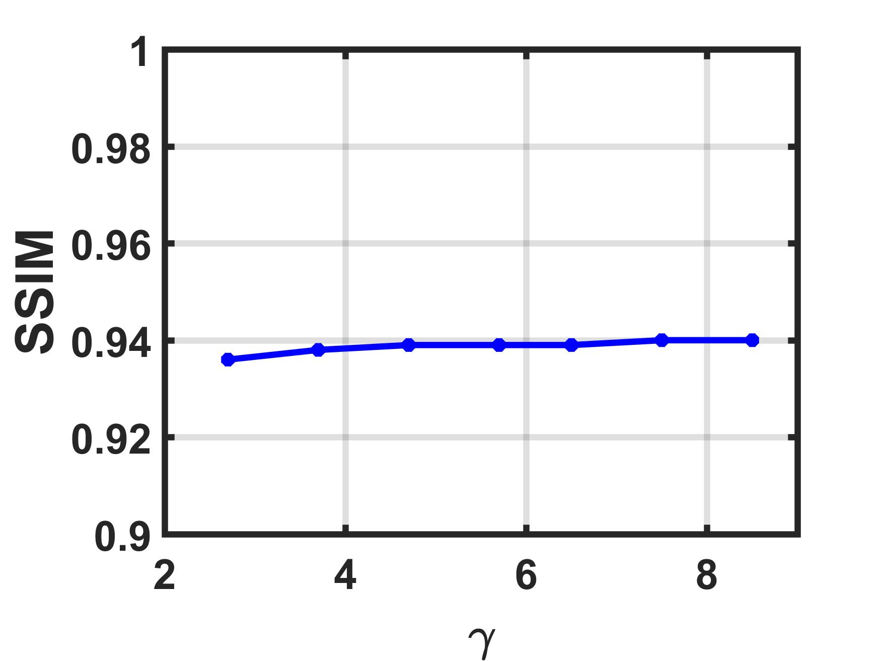
(f) SR=0.1

Figure 19: Sensitivity analysis of parameter $\gamma$ in HSI dataset. (a-c) Change in the MPSNR value: SR= 0.025, 0.05 and 01. (e-f) Change in the MSSIM value: 0.025, 0.05 and 0.1, respectively.

TABLE V: Parameters setting in the proposed algorithm

		Vdieo-suzie			Video-hall			MRI dataset			HSI dataset
SR	0.05	0.1	0.2	0.05	0.1	0.2	0.05	0.1	0.2	0.025	0.05	0.1
$\gamma$	2.3	2.5	2.7	1.7	2.6	2.6	1.3	2.5	3.0	3.5	5.5	5.7

V-D Discussion

Considering the fact that the $\gamma$ in $\mathbf{X}_{n}$ and $\mathbf{A}_{n}$ have certain proportional relationship, we simply set the $\gamma$ in $\mathbf{X}_{n}$ as 0.1, and tune the $\gamma$ in $\mathbf{A}_{n}$ carefully. For experiments on video datasets , MRI and HSI dataset, Fig. 17, Fig. 18 and Fig. 19 show the effect of parameter $\gamma$ on PSNR and SSIM at different sampling rates, respectively. To enhance the repeatability of our model, we list the optimal $\gamma$ of various datasets at different sampling rates in Table V. In addition, we manually set both $\tau_{n}$ and $\lambda_{n}$ as 0.01.

VI Conclusions

In this paper, we propose a novel double low-rank tensor model based on multi-mode matrix decomposition for tensor completion. Instead of using the traditional single nuclear norm or its relaxation to represent the low-rank prior of underlying tensor directly, we first apply parallel matrix factorization to all modes of underlying tensor, then, a novel double nonconvex $L_{\gamma}$ norm is designed to represent the underlying joint-manifold drawn from the mode factorization factors. An BSUM based algorithm is designed to efficiently solve the proposed model, and it can be demonstrated that our numerical scheme converges to the coordinatewise minimizers. The proposed model has been evaluated on three types of public tensor datasets, which show that our algorithm can complete a variety of low-rank tensors with significantly fewer samples than the compared methods.

References

- [1] K. A. Patwardhan, G. Sapiro, and M. Bertalmío, “Video inpainting under constrained camera motion,” IEEE Transactions on Image Processing, vol. 16, no. 2, pp. 545–553, 2007.
- [2] J. Yuan, “Mri denoising via sparse tensors with reweighted regularization,” Applied Mathematical Modelling, vol. 69, pp. 552–562, 2019.
- [3] B. Yaman, S. Weingärtner, N. Kargas, N. D. Sidiropoulos, and M. Akçakaya, “Low-rank tensor models for improved multi-dimensional mri: Application to dynamic cardiac t1 mapping,” IEEE Transactions on Computational Imaging, 2019.
- [4] A. C. Sauve, A. O. Hero, W. L. Rogers, S. J. Wilderman, and N. H. Clinthorne, “3d image reconstruction for a compton spect camera model,” IEEE Transactions on Nuclear Science, vol. 46, no. 6, pp. 2075–2084, 1999.
- [5] J. Tachella, Y. Altmann, M. Márquez, H. Arguello-Fuentes, J. Tourneret, and S. McLaughlin, “Bayesian 3d reconstruction of subsampled multispectral single-photon lidar signals,” IEEE Transactions on Computational Imaging, vol. 6, pp. 208–220, 2020.
- [6] H.-J. Zeng, X.-Z. Xie, K. Wen-Feng, S. Cui, and J.-F. Ning, “Hyperspectral image denoising via combined non-local self-similarity and local low-rank regularization,” IEEE Access, vol. 8, pp. 50 190–50 208, 2020.
- [7] Y. Chen, S. Wang, and Y. Zhou, “Tensor nuclear norm-based low-rank approximation with total variation regularization,” IEEE Journal of Selected Topics in Signal Processing, vol. 12, no. 6, pp. 1364–1377, 2018.
- [8] J.-T. Sun, H.-J. Zeng, H. Liu, Y. Lu, and Z. Chen, “Cubesvd: a novel approach to personalized web search,” in Proceedings of the 14th international conference on World Wide Web, 2005, pp. 382–390.
- [9] N. Kreimer and M. D. Sacchi, “A tensor higher-order singular value decomposition for prestack seismic data noise reduction and interpolation,” Geophysics, vol. 77, no. 3, pp. V113–V122, 2012.
- [10] C. Lu, J. Feng, Y. Chen, W. Liu, Z. Lin, and S. Yan, “Tensor robust principal component analysis with a new tensor nuclear norm,” IEEE Transactions on Pattern Analysis and Machine Intelligence, vol. 42, no. 4, pp. 925–938, 2019.
- [11] Z. Wen, W. Yin, and Y. Zhang, “Solving a low-rank factorization model for matrix completion by a nonlinear successive over-relaxation algorithm,” Mathematical Programming Computation, vol. 4, no. 4, pp. 333–361, 2012.
- [12] R. A. Harshman and M. E. Lundy, “Parafac: Parallel factor analysis,” Computational Statistics & Data Analysis, vol. 18, no. 1, pp. 39–72, 1994.
- [13] L. R. Tucker, “Some mathematical notes on three-mode factor analysis,” Psychometrika, vol. 31, no. 3, pp. 279–311, 1966.
- [14] H. Zeng, X. Xie, H. Cui, Y. Zhao, and J. Ning, “Hyperspectral image restoration via cnn denoiser prior regularized low-rank tensor recovery,” Computer Vision and Image Understanding, vol. 197-198, p. 103004, 2020.
- [15] M. E. Kilmer, K. Braman, N. Hao, and R. C. Hoover, “Third-order tensors as operators on matrices: A theoretical and computational framework with applications in imaging,” SIAM Journal on Matrix Analysis and Applications, vol. 34, no. 1, pp. 148–172, 2013.
- [16] M. Ding, T.-Z. Huang, T.-Y. Ji, X.-L. Zhao, and J.-H. Yang, “Low-rank tensor completion using matrix factorization based on tensor train rank and total variation,” Journal of Scientific Computing, vol. 81, no. 2, pp. 941–964, 2019.
- [17] H. Huang, Y. Liu, and C. Zhu, “Low-rank tensor completion via tensor ring with balanced unfolding,” arXiv preprint arXiv:1903.03315, 2019.
- [18] J. Liu, P. Musialski, P. Wonka, and J. Ye, “Tensor completion for estimating missing values in visual data,” IEEE Transactions on Pattern Analysis and Machine Intelligence, vol. 35, no. 1, pp. 208–220, 2012.
- [19] H. Kong and Z. Lin, “Tensor q-rank: A new data dependent tensor rank,” arXiv preprint arXiv:1910.12016, 2019.
- [20] C. Lu, J. Tang, S. Yan, and Z. Lin, “Generalized nonconvex nonsmooth low-rank minimization,” in Proceedings of the IEEE Conference on Computer Vision and Pattern Recognition, 2014, pp. 4130–4137.
- [21] F. Shang, J. Cheng, Y. Liu, Z.-Q. Luo, and Z. Lin, “Bilinear factor matrix norm minimization for robust pca: Algorithms and applications,” IEEE Transactions on Pattern Analysis and Machine Intelligence, vol. 40, no. 9, pp. 2066–2080, 2017.
- [22] T.-X. Jiang, T.-Z. Huang, X.-L. Zhao, and L.-J. Deng, “Multi-dimensional imaging data recovery via minimizing the partial sum of tubal nuclear norm,” Journal of Computational and Applied Mathematics, vol. 372, p. 112680, 2020.
- [23] J. Xue, Y. Zhao, W. Liao, and J. C.-W. Chan, “Nonconvex tensor rank minimization and its applications to tensor recovery,” Information Sciences, vol. 503, pp. 109–128, 2019.
- [24] W. Cao, Y. Wang, C. Yang, X. Chang, Z. Han, and Z. Xu, “Folded-concave penalization approaches to tensor completion,” Neurocomputing, vol. 152, pp. 261–273, 2015.
- [25] E. J. Candes, M. B. Wakin, and S. P. Boyd, “Enhancing sparsity by reweighted l1 minimization,” Journal of Fourier Analysis and Applications, vol. 14, no. 5-6, pp. 877–905, 2008.
- [26] T.-Y. Ji, T.-Z. Huang, X.-L. Zhao, T.-H. Ma, and L.-J. Deng, “A non-convex tensor rank approximation for tensor completion,” Applied Mathematical Modelling, vol. 48, pp. 410–422, 2017.
- [27] M. Lysaker, S. Osher, and X.-C. Tai, “Noise removal using smoothed normals and surface fitting,” IEEE Transactions on Image Processing, vol. 13, no. 10, p. 1345, 2004.
- [28] M. Burger, G. Gilboa, S. Osher, and J. Xu, “Nonlinear inverse scale space methods,” Communications in Mathematical Sciences, vol. 4, no. 1, pp. 179–212, 2006.
- [29] Y. Lou, P. Yin, Q. He, and J. Xin, “Computing sparse representation in a highly coherent dictionary based on difference of and ,” Journal of Scientific Computing, vol. 64, no. 1, pp. 178–196, 2015.
- [30] Y. Chen, Y. Guo, Y. Wang, D. Wang, C. Peng, and G. He, “Denoising of hyperspectral images using nonconvex low rank matrix approximation,” IEEE Transactions on Geoscience and Remote Sensing, vol. 55, no. 9, pp. 5366–5380, 2017.
- [31] Y. Xu, R. Hao, W. Yin, and Z. Su, “Parallel matrix factorization for low-rank tensor completion,” arXiv preprint arXiv:1312.1254, 2013.
- [32] T.-Y. Ji, T.-Z. Huang, X.-L. Zhao, T.-H. Ma, and G. Liu, “Tensor completion using total variation and low-rank matrix factorization,” Information Sciences, vol. 326, pp. 243–257, 2016.
- [33] Z. Zhang and S. Aeron, “Exact tensor completion using t-svd,” IEEE Transactions on Signal Processing, vol. 65, no. 6, pp. 1511–1526, 2016.
- [34] H. Zhang, J. Yang, F. Shang, C. Gong, and Z. Zhang, “Lrr for subspace segmentation via tractable schatten- norm minimization and factorization,” IEEE Transactions on Cybernetics, vol. 49, no. 5, pp. 1722–1734, 2018.
- [35] J. M. Bioucas-Dias, A. Plaza, N. Dobigeon, M. Parente, Q. Du, P. Gader, and J. Chanussot, “Hyperspectral unmixing overview: Geometrical, statistical, and sparse regression-based approaches,” IEEE Journal of Selected Topics in Applied Earth Observations and Remote Sensing, vol. 5, no. 2, pp. 354–379, 2012.
- [36] M. Razaviyayn, M. Hong, and Z.-Q. Luo, “A unified convergence analysis of block successive minimization methods for nonsmooth optimization,” SIAM Journal on Optimization, vol. 23, no. 2, pp. 1126–1153, 2013.
- [37] C. Lu, J. Tang, S. Yan, and Z. Lin, “Nonconvex nonsmooth low rank minimization via iteratively reweighted nuclear norm,” IEEE Transactions on Image Processing, vol. 25, no. 2, pp. 829–839, 2015.
- [38] S. Gaïffas and G. Lecué, “Weighted algorithms for compressed sensing and matrix completion,” arXiv preprint arXiv:1107.1638, 2011.
- [39] Q. Huynh-Thu and M. Ghanbari, “Scope of validity of psnr in image/video quality assessment,” Electronics Letters, vol. 44, no. 13, pp. 800–801, 2008.
- [40] Z. Wang, A. C. Bovik, H. R. Sheikh, E. P. Simoncelli et al., “Image quality assessment: from error visibility to structural similarity,” IEEE Transactions on Image Processing, vol. 13, no. 4, pp. 600–612, 2004.
- [41] L. Zhang, L. Zhang, X. Mou, and D. Zhang, “FSIM: A feature similarity index for image quality assessment,” IEEE Transactions on Image Processing, vol. 20, no. 8, pp. 2378–2386, 2011.
- [42] L. Wald, Data fusion: definitions and architectures: fusion of images of different spatial resolutions. Presses des MINES, 2002.
- [43] F. Kruse, A. Lefkoff, and J. Dietz, “Expert system-based mineral mapping in northern death valley, california/nevada, using the airborne visible/infrared imaging spectrometer (aviris),” Remote Sensing of Environment, vol. 44, no. 2-3, pp. 309–336, 1993.